Effects of viscoelasticity on shear-thickening in dilute suspensions in a viscoelastic fluid

Abstract

We investigate previously unclarified effects of fluid elasticity on shear-thickening in dilute suspensions in an Oldroyd-B viscoelastic fluid using a novel direct numerical simulation based on the smoothed profile method. Fluid elasticity is determined by the Weissenberg number $Wi$ and by viscosity ratio $1-\beta=\eta_{p}/(\eta_{s}+\eta_{p})$ which measures the coupling between the polymer stress and flow: $\eta_{p}$ and $\eta_{s}$ are the polymer and solvent viscosity, respectively. As $1-\beta$ increases, while the stresslet does not change significantly compared to that in the $\beta\to 1$ limit, the growth rate of the normalized polymer stress with $Wi$ was suppressed. Analysis of flow and conformation dynamics around a particle for different $\beta$ reveals that at large $1-\beta$, polymer stress modulates flow, leading to suppression of polymer stretch. This effect of $\beta$ on polymer stress development indicates complex coupling between fluid elasticity and flow, and is essential to understand the rheology and hydrodynamic interactions in suspensions in viscoelastic media.

I Introduction

Particle suspensions in viscoelastic fluids, such as polymer solutions or polymer melts, are widely used in industrial products. To handle such suspensions effectively and efficiently, understanding their rheology is essential. However, the influence of the media’s viscoelasticity on suspension rheology is not well understood. One type of viscoelastic fluids, so-called Boger fluids, are widely utilized to examine the effect of fluid elasticity due to constant shear viscosity. Experimental studies have reported that the apparent viscosity of suspensions in Boger fluids shear-thickens even at dilute particle volume fractions Zarraga2001 ; Scirocco2005 ; Tanner2013 , suggesting complex interactions between the viscoelastic medium and suspended particles. Scirocco et al. Scirocco2005 reported the thickening at $\phi_{p}=0.068$. Zarraga et al. Zarraga2001 and Dai et al. Tanner2013 did not explicitly mention the thickening at low $\phi_{p}$ conditions. However, their data at $\phi_{p}=0.3$ Zarraga2001 and $\phi_{p}=0.05$ Tanner2013 indicates mild shear-thickening.

Recently, to understand the mechanisms of this thickening, the rheology of a dilute suspension in an Oldroyd-B fluid have been studied theoretically and numerically Koch2016 ; Yang2016 ; Einarsson2018 ; Yang2018 ; Yang2018a . The Oldroyd-B fluid is one of the simplest constitutive models of viscoelastic fluids such as polymer solutions Bird1987 . The shear viscosity and the first normal stress difference (NSD) coefficient of an Oldroyd-B fluid are independent of the applied shear rate $\dot{\gamma}$. This rate-independent shear viscosity combined with finite elasticity is desirable for modeling the steady shear behavior of Boger fluids. Although the Oldroyd-B fluid can not capture the whole rheological behavior of real viscoelastic fluids due to it’s simplicity James2009 , from another point of view, it’s simplicity is helpful to obtain a fundamental insight into the separate effects of elasticity and shear viscosity. Elasticity of Oldroyd-B fluids is characterized by two parameters: relaxation time $\lambda$ and viscosity ratio $\beta=\eta_{s}/\eta_{0}$, where $\eta_{s}$ and $\eta_{p}$ are the viscosity of the solvent and polymer, respectively, and $\eta_{0}=\eta_{s}+\eta_{p}$ is the zero-shear viscosity. By definition, $0\leq\beta\leq 1$. Here, a small $\beta$ corresponds to a high polymer concentration or a high-molecular-weight polymer, indicating strong fluid elasticity Bird1987 . The Weissenberg number $Wi=\lambda\dot{\gamma}$ measures the viscoelasticity strength under an applied rate of $\dot{\gamma}$ irrespective of $\beta$. Koch et al. Koch2016 and Einarsson et al. Einarsson2018 applied the perturbation theory and demonstrated that the suspension viscosity of Oldroyd-B fluid shear thickens. Yang et al. numerically simulated a previously reported system Einarsson2018 and concluded that the particle-induced fluid stress around the particles is the primary source of suspension shear-thickening Yang2016 ; Yang2018 .

In studies about flow-induced particle clustering in viscoelastic fluids, the fluid elasticity is characterized by the elastic parameter $S_{R}=N_{1}/(2\sigma_{xy})$, where $N_{1}$ and $\sigma_{xy}$ are the first NSD and the shear stress, respectively Scirocco2004 ; Won2004 ; Pasquino2010 ; Hwang2011 ; SantosdeOliveira2011 ; SantosdeOliveira2012 ; Choi2012 ; Pasquino2013 ; VanLoon2014 ; Pasquino2014 ; Jaensson2016 . For Oldroyd-B fluids, $S_{R}=(1-\beta)Wi$, which suggests that not only $Wi$ but also $1-\beta$ increase the clustering tendency. The question is whether this trend can also explain the shear-thickening of suspensions in viscoelastic fluids; do both $1-\beta$ and $Wi$ enhance the shear-thickening? While the positive effect of $Wi$ on shear-thickening has been revealed in recent studies Koch2016 ; Yang2016 ; Einarsson2018 ; Yang2018 ; Yang2018a , the detailed effect of $\beta$ remains unclear. The theories by Koch et al. Koch2016 and Einarsson et al. Einarsson2018 are perturbation theories with the polymer concentration and $Wi$, respectively. Thus at high $S_{R}$ conditions where $1-\beta$ and $Wi$ are both large, these theories are inadaptable. To evaluate the nonlinear suspension behavior at large $S_{R}$ conditions, we need to conduct numerical calculations which fully solve the governing equations. The numerical studies by Yang and Shaqfeh Yang2018 mainly focused on the thickening mechanism at $\beta\to 1$ condition, where the feedback of the polymer stress to the flow can be ignored, i.e. flow field is not perturbed by the polymer stress. In such extreme conditions, since the polymer stress can be analyzed separately from the flow field, analytic perturbation theories have been developed Koch2016 ; Einarsson2018 , and then examined by numerical calculations Yang2018 . However, real viscoelastic fluids used for industrial purposes show the finite polymer concentrations, where the coupling between the polymer stress and flow represented by $\beta$ value should be more important. Therefore, to understand the thickening mechanism in general viscoelastic suspensions, the effects of $\beta$ need to be clarified. Yang and Shaqfeh showed the change in the $Wi$-dependence of the shear-thickening in polymer stress at a moderate $\beta$ value of 0.68, and only mentioned the effects of flow modulation by large polymer stressYang2018 ; however, the underlying $\beta$ dependence of flow and polymer stress was not analyzed. For situations where the polymer stress and the flow field strongly couples, physics of shear-thickening in viscoelastic suspensions was not fully explored.

On these backgrounds, the purpose of this article is to clarify the effects of fluid’s viscoelasticity, specifically the coupling between the polymer stress and flow in a wide range of $Wi$, on the shear-thickening of the suspensions in Oldroyd-B fluids. We first briefly explain our newly developed numerical method. Then, we present the calculation results of suspension viscosity and NSD coefficient, which indicate the non-trivial effect of $\beta$ on shear-thickening. Finally, the mechanism of this effect is investigated through interactions between stress and flow fields around the particles.

II Simulation method

II.1 Governing equations

Several direct numerical simulations (DNS), which use the fluid mesh independent of the surface boundaries of particles rather than body-fitted mesh Ahamadi2008 ; Ahamadi2010 ; Choi2010 ; Choi2012 ; Jaensson2015 ; Jaensson2016 ; Yang2016 ; Yang2018 , and particle based methods, which express a viscoelastic fluid as discrete fluid particles, have been adapted for suspensions in a viscoelastic fluid in 2D Hwang2004 ; Hwang2011 ; Pasquino2014 and 3D space SantosdeOliveira2011 ; SantosdeOliveira2012 ; DAvino2013 ; Vazquez-Quesada2017 ; Krishnan2017 ; Yang2018a ; Vazquez-Quesada2019 . One of the authors proposed the smoothed profile method (SPM), an efficient DNS for suspensions in which interaction between particles and the medium is treated through the smoothed profile function Nakayama2005 ; Nakayama2008 . In SPM, regular mesh rather than body-fitted mesh can be used; therefore, the calculation cost of fluid fields, which is dominant in total calculation costs, is nearly independent of the particle numberNakayama2008 . This is advantageous for simulation of dense suspensions that containing many particles. For examples, using SPM, the shear viscosity Iwashita2009 ; Kobayashi2011 ; Molina2016 and complex modulus Iwashita2010 and particle coagulation rate Matsuoka2012 of Brownian suspensions up to $\phi_{p}\leq 0.56$ in Newtonian fluids were efficiently evaluated. Application of SPM was extended to complex host fluids, such as electrolyte solutions Kim2006 ; Nakayama2008 ; luo2010modeling and to active swimmer suspensions Molina2013 . Since it can be applied to any continuum solvers, SPM combined with the lattice-Boltzmann method for a viscoelastic fluid has been reported Lee2017 . In this study, we developed a DNS with SPM that efficiently evaluates the bulk rheology of suspension in a viscoelastic fluid in 3D space.

We consider the suspension of neutrally buoyant and non-Brownian $N$ spherical particles with radius $a$, mass $M_{p}$, and moment of inertia $\bm{I}_{p}$ in a viscoelastic fluid. Hereafter unless otherwise stated, all the physical quantities are non-dimensionalized by length unit $a$, velocity unit $a\dot{\gamma}$, and stress unit $\eta_{0}\dot{\gamma}$. Hence, $M_{p}$ and $\bm{I}_{p}$ are non-dimensionalized as $\tilde{M}_{p}=M_{p}\dot{\gamma}/(\eta_{0}a)$ and $\tilde{\bm{I}}_{p}=\bm{I}_{p}\dot{\gamma}/(\eta_{0}a^{3})$, respectively.

Non-dimensional velocity field $\bm{u}(\bm{r},t)$ at position $\bm{r}$ and time $t$ is governed as follows:

$$Re\left(\frac{\partial}{\partial t}+\bm{u}\cdot\nabla\right)\bm{u} = \nabla\cdot(\bm{\sigma}_{n}+\bm{\sigma}_{p})+Re\phi\bm{f}_{p},$$ (1)

$$\nabla\cdot\bm{u} = 0,$$ (2)

where $Re=\rho a^{2}\dot{\gamma}/\eta_{0}$, $\rho$, $\bm{\sigma}_{n}=-p\bm{I}+2\beta\bm{D}$, $\bm{\sigma}_{p}$, $\bm{I}$, $\bm{D}=(\nabla\bm{u}+\nabla\bm{u}^{T})/2$, and $p$ are the Reynolds number, fluid mass density, Newtonian solvent stress, and polymer stress, unit tensor, strain-rate tensor, and pressure, respectively. In SPM, The particle profile field is introduced as $\phi(\bm{r},t)\equiv\sum_{i=1}^{N}\phi_{i}$, where $\phi_{i}\in[0,1]$ is the $i$th particle profile function having continuous diffuse interface with thickness $\xi$ and indicating the inside and outside of particles by $\phi=0$ and $\phi=1$, respectively Nakayama2008 . The total velocity field $\bm{u}$ is given by

$$\bm{u}(\bm{r},t)=(1-\phi)\bm{u}_{f}+\phi\bm{u}_{p}$$ (3)

where $\bm{u}_{f}$ and $\bm{u}_{p}$ are the fluid and particle velocity fields, respectively. The body force $\phi\bm{f}_{p}$ enforces particle rigidity in the velocity field, which is defined in the temporal discretization of Eq. (1) Nakayama2008 ; Molina2016 . The time-integrated body force $\phi\bm{f}_{p}$ is calculated as

$$\int_{t}^{t+\Delta t}\phi\bm{f}_{p}ds=\phi(\bm{u}_{p}-\bm{u}^{*})$$ (4)

where $\Delta t$ is the simulation time step and $\bm{u}^{*}$ is the adjacent intermediate total velocity field updated using Eq. (1) without the last term in the fractional time stepping.

The individual particles evolve by

$$\dot{\bm{R}}_{i} = \bm{V}_{i},$$ (5)

$$\tilde{M}_{p}\dot{\bm{V}}_{i} = \bm{F}^{H}_{i}+\bm{F}^{C}_{i},$$ (6)

$$\tilde{\bm{I}}_{p}\cdot\dot{\bm{\Omega}}_{i} = \bm{N}^{H}_{i},$$ (7)

where $\bm{R}_{i}$, $\bm{V}_{i}$, and $\bm{\Omega}_{i}$ are the position, velocity and angular velocity of the $i$th particle, respectively. $\bm{F}_{i}^{H},\bm{N}_{i}^{H}$ Nakayama2008 ; Molina2016 are the hydrodynamic force and torque, respectively, and $\bm{F}_{i}^{C}$ is a potential force due to the excluded volume that prevents particles from overlapping. The hydrodynamic force $\bm{F}_{i}^{H},\bm{N}_{i}^{H}$ are determined by Newton’s third law of motion:

$$\int_{t}^{t+\Delta t}\bm{F}_{i}^{H}ds = \int Re\phi_{i}(\bm{u}^{*}-\bm{u}_{p}^{*})d\bm{r},$$ (8)

$$\int_{t}^{t+\Delta t}\bm{N}_{i}^{H}ds = \int\bm{r}_{i}\times Re\phi_{i}(\bm{u}^{*}-\bm{u}_{p}^{*})d\bm{r}$$ (9)

where $\bm{u}_{p}^{*}$ is the intermediate particle velocity field freely advected by the previous particle velocity and $\bm{r}_{i}=\bm{r}-\bm{R_{i}}$. The particle velocity field $\bm{u}_{p}$ is calculated as

$$\phi\bm{u}_{p}=\sum_{i=1}^{N}\phi_{i}\left[\bm{V}_{i}+\bm{\Omega}_{i}\times\bm{r}_{i}\right].$$ (10)

The detail computational algorithm about the fractional time stepping is elaborated on in Refs. Nakayama2008 ; Molina2016 .

For polymer stress, we use Oldroyd-B fluid:

$$\left(\frac{\partial}{\partial t}+\bm{u}\cdot\nabla\right)\bm{C} = (\nabla\bm{u})^{T}\cdot\bm{C}+\bm{C}\cdot(\nabla\bm{u})-\frac{\bm{C}-\bm{I}}{Wi},$$ (11)

$$\bm{\sigma}_{p} = \frac{(1-\beta)(\bm{C}-\bm{I})}{Wi},$$ (12)

where $\bm{C}(\bm{r},t)$ is the conformation tensor. Oldroyd-B fluid microscopically corresponds to a dilute suspension of dumbbells with a linear elastic spring in an Newtonian solvent Bird1987 . Conformation tensor $\bm{C}$ is expressed as $C_{ij}=\langle X_{i}X_{j}\rangle$, where $\bm{X}$ is the dumbbell’s end to end vector normalized by the radius of gyration of polymer and $\langle\cdot\rangle$ is the ensemble average. The average stretch and orientation of dumbbells are $\mathrm{tr}\bm{C}-3$ and the major orientation of $\bm{C}$, respectively. The deformation and orientation of $\bm{C}$ determine the polymer stress. When $\bm{C}=\bm{I}$, polymer stress is zero in the completely relaxed state. For shear stress component, $\sigma_{p,xy}=(1-\beta)/(2Wi)\langle\bm{X}^{2}\sin{2\theta}\rangle$, where $\theta$ is the dumbbell’s orientation angle from the shear flow direction. As explained later, this dumbbell representation of $\bm{C}$ is effectively interpreted using novelly introduced conformation ellipsoid that is constructed by the eigenvalues and eigenvectors of $\bm{C}$. The polymer stress modulates the flow through $\nabla\cdot\bm{\sigma}_{p}$ in Eq. (1). Eventually, the balance between viscous and polymer stresses, and external shear driving results in the steady state.

II.2 Stress calculation

The instantaneous volume-averaged stress of the suspension is evaluated in SPM Nakayama2008 ; Iwashita2009 ; Molina2016 by

$$\bm{\sigma}^{\rm sus}=\frac{1}{V}\int_{V}[\bm{\sigma}_{n}+\bm{\sigma}_{p}-\bm{r}Re\phi\bm{f}_{p}+\bm{ru}\cdot\nabla(Re\bm{u})]d\bm{r},$$ (13)

where $V$ is the total volume of system and the last term on the right hand side comes from the convective momentum-flux tensor, which is negligible on time averaging over the steady state Iwashita2009 . By assuming ergodicity, the ensemble average of the stress $\langle\bm{\sigma}^{\rm sus}\rangle$ is equated to the average over time.

In suspension rheology, the stress decomposition has been utilized for the evaluation of each contribution of stress components. In this study, we adopt the procedure proposed by Yang et al. Yang2016 as follows,

$$\langle\bm{\sigma}^{\rm sus}\rangle = \langle\bm{\sigma}^{F0}\rangle+\frac{N}{V}(\langle\bm{\Sigma}\rangle+\langle\bm{S}\rangle),$$ (14)

$$\bm{\Sigma} = \frac{1}{N}\int_{V}(\bm{\sigma}^{F}-\bm{\sigma}^{F0})\mathrm{d}\bm{r},$$ (15)

$$\bm{S} = \frac{1}{N}\int_{S_{p}}(\bm{r}(\bm{n}\cdot\bm{\sigma}^{F}))^{sym}\mathrm{d}S,$$ (16)

where $\bm{\sigma}^{F}$ is the stress in the fluid region, $\bm{\sigma}^{F0}$ is the fluid stress without particles under the simple shear flow, $S_{p}$ is the surface of particles, and $(\bm{A})^{sym}$ denotes the symmetric part of tensor $\bm{A}$. $\bm{\Sigma}$ represents the stress induced by one particle inclusion in the fluid region, and $\bm{S}$ is the stresslet. Evaluation of Eqs. (15)-(16) requires surface or volume integrals. To calculate these integrals numerically in the immersed boundary method, appropriate location of the particle-fluid interface should be carefully examined Yang2018a . By contrast, in SPM, due to the diffuse interface of the smoothed profile function, the integrals in Eqs. (15)-(16) are simply evaluated as follows,

$$\bm{\Sigma} \approx \frac{1}{N}\int_{V}[(\bm{\sigma}_{n}+\bm{\sigma}_{p})^{F}-(\bm{\sigma}_{n}+\bm{\sigma}_{p})^{F0}]d\bm{r},$$ (17)

$$\bm{S} \approx -\frac{1}{N}\int_{V}\bm{r}Re\phi\bm{f}_{p}d\bm{r}.$$ (18)

The numerical results by our simple formalism of stress decomposition reasonably agree with those by body-fitted mesh method Yang2018 as seen later.

For convenience, viscometric functions are non-dimensionalized as, $\eta\equiv\langle\sigma^{\rm sus}_{xy}\rangle$ and $\Psi_{1}\equiv\langle\sigma^{\rm sus}_{xx}-\sigma^{\rm sus}_{yy}\rangle/Wi$, and are also decomposed to each contributions as follows Yang2016 ; Yang2018 ; Yang2018a ,

$$\eta = \eta^{0}+\frac{N}{V}\eta^{p},$$ (19)

$$\Psi_{1} = \Psi_{1}^{0}+\frac{N}{V}\Psi_{1}^{p},$$ (20)

where $\eta^{0}\equiv\langle\sigma_{xy}^{F0}\rangle$ and $\Psi_{1}^{0}\equiv\langle\sigma_{xx}^{F0}-\sigma_{yy}^{F0}\rangle/Wi$ are the non-dimensional fluid viscosity and first NSD coefficient without particles. Note that the NSD coefficient is normalized by $\eta_{0}\lambda$ rather than $\Psi_{1,0}=2\eta_{p}\lambda$, which is the NSD coefficient of a Oldroyd-B fluid without particles, since our units of the stress and rate are $\eta_{0}\dot{\gamma}$ and $Wi$, respectively. $\eta^{p}$ and $\Psi_{1}^{p}$ are the particle contributions to the suspension viscosity and first NSD coefficient, respectively;

$$\eta^{p} \equiv \langle\Sigma_{xy}\rangle+\langle S_{xy}\rangle,$$ (21)

$$\Psi_{1}^{p} \equiv \frac{\langle\Sigma_{xx}-\Sigma_{yy}\rangle+\langle S_{xx}-S_{yy}\rangle}{Wi},$$ (22)

where $\bm{\Sigma}$ and $\bm{S}$ are non-dimensionalized by $\eta_{0}\dot{\gamma}a^{3}$.

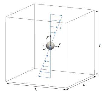
Figure 1: Schematic for the simulated system. The shear flow, shear gradient and vorticity directions are along with Cartesian x, y, z-axes, respectively. Periodic boundary conditions are imposed on all faces of the cubic system.

II.3 Numerical implementation

To impose the simple shear flow on the system, we use the time-dependent oblique coordinate evolving with mean shear velocity as $\bm{r}(t)=\bm{r}(0)-\dot{\gamma}ty\bm{e}_{x}$ and solve evolution equations (Eqs. (1)-(2), (11)-(12)) formulated on the moving coordinate Luo2004 ; Venturi2009 ; Kobayashi2011 ; Molina2016 , where $\bm{e}_{x}$ is a Cartesian x-axis basis vector. The particle equations (Eqs. (5)-(7)) are solved under Lees-Edwards boundary conditions Kobayashi2011 ; Molina2016 . This formulation enables us to impose the full periodic boundary condition and evaluate the bulk rheological properties of the suspension without wall effects. The similar full periodic boundary conditions were adopted for steady shear 2D simulations Hwang2004 ; Jaensson2015 and dynamic shear 3D simulations DAvino2013 of viscoelastic suspensions. To the best of our knowledge, this study is the first to report the steady shear simulation of a full periodic 3D system of viscoelastic suspensions.

The evolution equations are solved using the spectral method, which naturally matches the full periodic boundary condition. The stability condition given by the momentum diffusion term is adopted for determining the simulation time step; $\Delta t=\rho/\eta_{0}K_{max}^{2}$ ($K_{max}$ is the largest wave number in our spectral scheme).

III Results and discussion

III.1 Simulation conditions

In this study, we focus on a dilute suspension condition. As Figure 1 shows, one particle is located at the center of the cubic box $[-L/2,L/2]^{3}$, where $L=128\Delta$ is the system length and $\Delta$ is the lattice length. The mesh resolutions of particles are $a=8\Delta$ and $\xi=2\Delta$. In this setup, the particle volume fraction $\phi_{p}=0.00102$. This very dilute condition is hardly achieved experimentally. However, such dilute condition, where the complex inter-particle effects are negligible, is preferable to examine the fundamental effect of the interaction between the medium and one particle. Now that we treat only one particle ($N=1$), the inter-particle force $\bm{F}^{C}$ in Eq. (5) can be ignored. Simple shear flow is imposed on the whole system and then the viscometric functions of suspensions at steady states are evaluated.

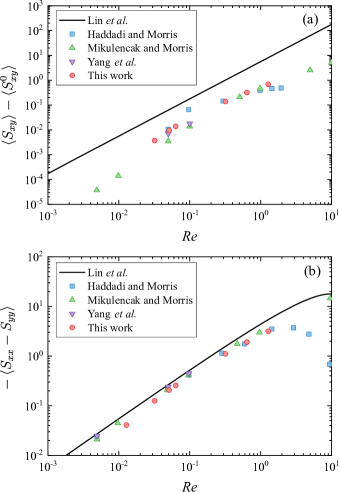
Figure 2: Each component of stresslets in a dilute suspension in a Newtonian medium as a function of $Re$: (a) shear component $\langle S_{xy}\rangle$ (b) the first NSD components $-\langle S_{xx}-S_{yy}\rangle$. In Fig. 2(a), the results at $Re=0.0128$ is used as the value of $\langle S_{xy}^{0}\rangle$. The past numerical simulation results MIKULENCAK2004 ; Haddadi2014 ; Yang2016 and theoretical lines LIN1970 are also displayed.

III.2 Validation of SPM for sheared viscoelastic suspension

In order to validate the SPM, we calculate the shear stress and NSD for $\beta=0.99$ case. For evaluation the stress of a viscoelastic suspension, inertial contribution to the stress is calculated first. Although the Reynolds number is set small ($Re\leq 0.0633$) to avoid the inertial effect, the inertial effect at a finite Reynolds number can not be ignored especially with the NSD components of suspension stresslets because both the inertial and non-inertial contributions to the NSD components are comparable. To remove finite inertial effects from viscometric evaluations, we follow the procedure proposed by Yang et al. Yang2016 . Figure 2 shows the Reynolds number dependence of each stresslet component in a Newtonian suspension calculated at the same system shown in Fig. 1. Our results agree well with the past numerical results MIKULENCAK2004 ; Haddadi2014 ; Yang2016 . In the evaluation for NSD of viscoelastic suspensions in the followings, the inertial contributions of stresslets at the corresponding Reynolds number conditions in Fig 2 are subtracted from the results of viscoelastic suspensions.

Next, the shear stress and first NSD for $\beta=0.99$ is examined. Comparison is reported in Fig. 3(b) for normalized viscosity and Fig. 5(b) for normalized first NSD coefficient. Our viscosity for $\beta=0.99$ is in good agreement with theoretical Einarsson2018 and numerical Yang2018 results (Fig. 3(b)). Our first NSD coefficient for $\beta=0.99$ also agrees with theoretical Koch2006 ; Greco2007 and numerical Yang2018 results (Fig. 5(b)). In the following, we discuss the cases with the strong flow-polymer stress coupling represented by finite $1-\beta$.

Figure 3: Suspension viscosity as a function of $\beta$ and $Wi$: (a) normalized viscosity $\eta_{r}$ (b) shear stress decomposition: stresslet (green), fluid stress (blue), stresslet+fluid stress (red). $\langle S_{xy,0}\rangle$ is the stresslet by Newtonian contribution at $Wi=0$. Different symbols are for $\beta=0.3(\blacklozenge),0.5(\blacksquare),0.8(\blacktriangle),0.99(\bullet)$. The crosses are from Yang and Shaqfeh’s DNS results ($\beta=0.99$) Yang2018 , and the dashed-line is the perturbation solution by Einarsson et al. ($\beta=0.99$) Einarsson2018 .

Figure 4: (Color online) Distribution of shear component of normalized polymer stress $\sigma_{p,xy}/(1-\beta)$ on shear plane ($xy$-plane) through the center of a particle. Positive contribution to shear-thickening is indicated by $\sigma_{p,xy}/(1-\beta)>1$ where the polymer shear stress is higher than $\eta_{p}\dot{\gamma}$. Solid lines show the streamlines. (a) $\beta=0.5,Wi=1$; (b) $\beta=0.99,Wi=1$; (c) $\beta=0.5,Wi=2$; (d) $\beta=0.99,Wi=2$.

III.3 The effects of $\beta$ on the suspension viscosity

Figure 3(a) shows the relative shear viscosity of a suspension $\eta_{r}=\eta=\langle\sigma_{xy}^{\rm sus}\rangle$ to $\eta_{0}$, as a function of $\beta$ and $Wi$. The relative apparent viscosity $\eta_{r}$ increases with $Wi$, which indicates shear-thickening. The shear-thickening is more pronounced for larger $1-\beta$, which is attributed to the relative increase of polymer stress contribution. To further investigate the origin of this shear-thickening, the particle contributions to suspension shear stress are decomposed according to Eq. (21) in Fig. 3(b). In Fig. 3(b), each stress component is additionally normalized by $1-\beta$, which represents the ratio of stress to $\eta_{p}\dot{\gamma}$ since now the normalization unit is $(1-\beta)\eta_{0}\dot{\gamma}=\eta_{p}\dot{\gamma}$. As $Wi$ increases, while $\langle S_{xy}\rangle$ shear-thins, $\langle\Sigma_{xy}\rangle$ strongly shear thickens; thus, summing them yields the total shear-thickening. Relative to the $\beta$ dependence shown in Fig. 3(b), we observe a non-trivial trend, i.e., thickening rate of $\langle\Sigma_{xy}\rangle/(1-\beta)$ for $Wi\gtrsim 1$ weakens at smaller $\beta$. This trend can also be observed in Fig. 3(a) as slower growth of $\eta_{r}$ with $Wi$ at smaller $\beta$. These results demonstrate that the growth of fluid elasticity with $1-\beta$ weakens the $Wi$-dependence in shear-thickening, which indicates that $1-\beta$ and $Wi$ in the elastic parameter $S_{R}$ have counteracting effects on shear-thickening in the suspension.

To evaluate the cause of the $\beta$-dependent thickening in $\langle\Sigma_{xy}\rangle$, Fig. 4 shows the distribution of polymer shear stress around a particle on the shear plane at $\beta=0.5$ and $0.99$. The case $\beta=0.99$ was already analyzed by Yang and Shaqfeh Yang2018 , who identified that the main source of $\langle\Sigma_{xy}\rangle$ thickening comes from polymer stress near the particle when the polymer stress is passive to the flow. Here, we discuss the effect of $1-\beta$ on the suspension rheology by comparing the cases of $\beta=0.5$ and $0.99$ cases. We observe localized large shear stress in the recirculation region near the particle (represented by the closed streamlines). For $Wi<1$, the distributions of the streamline and stress do not change significantly with $\beta$ (not shown). In contrast, for $Wi>1$, the level of polymer stress concentration in the recirculation region increases with larger $\beta$. In other words, the polymer shear stress concentration is suppressed with increased fluid elasticity with $1-\beta$. This change in polymer stress is reflected in the weakening of the $Wi$-dependence of shear-thickening in Fig. 3 and can be explained by the change in flow caused by the polymer stress. At $\beta=0.5$, the streamline visibly changes with $Wi$ (Figs. 4(a) and 4(c)), which demonstrates strong coupling between the polymer stress and the flow, while the streamline remains nearly unchanged between $Wi=1$ and $2$ at $\beta=0.99$ (Figs. 4(b) and 4(d)). These results clearly indicate that high fluid elasticity at the small $\beta$ condition modulates the flow, which suppresses local concentration of the polymer stress.

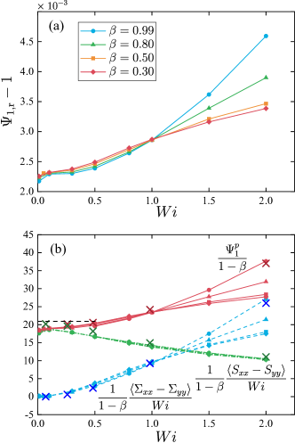
Figure 5: Suspension first NSD coefficient as a function of $\beta$ and $Wi$: (a) $\Psi_{1,r}$ (b) normal stress decomposition: stresslet (green), fluid stress (blue), stresslet+fluid stress (red). Different symbols are for $\beta=0.3(\blacklozenge),0.5(\blacksquare),0.8(\blacktriangle),0.99(\bullet)$. The crosses reference Yang and Shaqfeh’s DNS results ($\beta=0.99$) Yang2018 , and the dashed-line is the theoretical value of a second order fluid $\Psi_{1}^{p}/(1-\beta)=\langle\Sigma_{xx}-\Sigma_{yy}\rangle/((1-\beta)Wi)=20\pi/3$ Koch2006 ; Greco2007 .

The shear-thickening and it’s changes observed in this study might appear to be minor effects because the viscosity increment of this thickening is small (Fig. 3(a)). This is because that the particle concentration in this study is very dilute ($\phi_{p}=0.001$). We note that the shear-thickening in a viscoelastic suspension is qualitatively the result of the coupling between the flow and the viscoelastic response of a medium; modulated flow pattern from simple shear due to particle geometry induces extra viscoelasitic stress that further change the flow around the particle. This mechanism is supposed to be common in a wide class of viscoelastic suspensions; therefore, this effect is expected to work other systems regardless of the constitutive equation of a medium and/or the type of a particle. In addition, since the viscoelastic stress responsible for the shear-thickening occurs in the vicinity of particles (Fig. 4), this effect is supposed to be relevant and enhanced with particle concentration even in non-dilute suspensions where inter-particle interaction works. Furthermore, as explained later, the contribution of elongational flow around a particle (Fig. 8) suggests that the shear-thickening can become more prominent in viscoelastic media with strong elongational response.

III.4 The effects of $\beta$ on the first NSD coefficient

Figure 5(a) shows the relative first NSD coefficient of a suspension $\Psi_{1,r}=\Psi_{1}/(2(1-\beta))=\langle\sigma_{xx}^{\rm sus}-\sigma_{yy}^{\rm sus}\rangle/(2(1-\beta)Wi)$ to $\Psi_{1,0}=2\eta_{p}\lambda$, as a function of $\beta$ and $Wi$. As seen in $\eta_{r}$, $\Psi_{1,r}$ increases with $Wi$. The increasing rate of $\Psi_{1,r}$ for $Wi>1$ weakens at smaller $\beta$. In contrast to $\eta_{r}$, the enhancement of the first NSD coefficient for larger $1-\beta$ is not observed. This is simply because $\Psi_{1,0}$, which is the denominator of $\Psi_{1,r}$, purely originates from polymer stress and is also pronounced by the same order, $\Psi_{1,0}\propto\eta_{p}=\eta_{0}(1-\beta)$, as $\Psi_{1}$. As was done for the suspension viscosity, the suspension NSD is decomposed according to Eq. (22) in Fig. 5(b). The overall trend is similar to that in the suspension viscosity; as $Wi$ increases, while $\langle S_{xx}-S_{yy}\rangle$ decreases, $\langle\Sigma_{xx}-\Sigma_{yy}\rangle$ strongly increases.

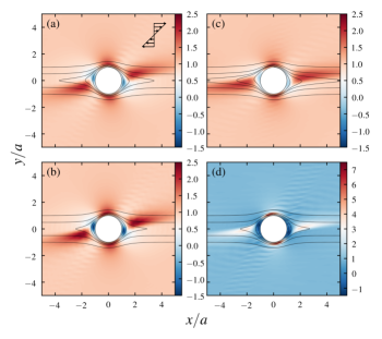
Figure 6: (Color online) Distribution of NSD component of normalized polymer stress $(\sigma_{p,xx}-\sigma_{p,yy})/(2(1-\beta)Wi)$ on shear plane ($xy$-plane) through the center of a particle. Positive contribution to shear increase is indicated by $(\sigma_{p,xx}-\sigma_{p,yy})/(2(1-\beta)Wi)>1$ where the polymer NSD is higher than $\Psi_{1,0}\dot{\gamma}^{2}$. Solid lines show the streamlines. (a) $\beta=0.5,Wi=1$; (b) $\beta=0.99,Wi=1$; (c) $\beta=0.5,Wi=2$; (d) $\beta=0.99,Wi=2$.

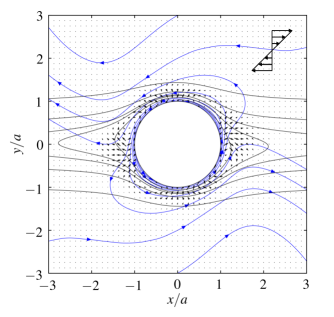
Figure 7: (Color online) Modulation of the velocity field at $\beta=0.5$ and $Wi=2$. The streamlines are calculated from velocity (black lines) and disturbance velocity $\delta\bm{u}$ (blue lines). The vector field indicates $\nabla\cdot\bm{\sigma}_{p}$.

Figure 6 shows the distribution of polymer NSD around a particle on the shear plane at $\beta=0.5$ and $0.99$. The general trend in Fig. 6 is the same as that in Fig. 4. For $Wi<1$, the distributions of NSD do not change significantly with $\beta$ (Figs. 6(a) and 6(b)). In contrast, for $Wi>1$, the level of polymer NSD concentration near the particle surface (especially at the poles of a particle) increases with $\beta$ (Fig. 6(d)). Note that the high NSD region (Fig. 6) extends more widely to the shear flow direction than the shear stress (Fig. 4). For smaller $\beta$ and larger $Wi$ conditions (Fig. 6(c)), high stress region extending outside of recirculation region near the particle surface, where polymers pass through the particle and more align to the flow direction, seems to give relatively higher contributions to total polymer NSD increase.

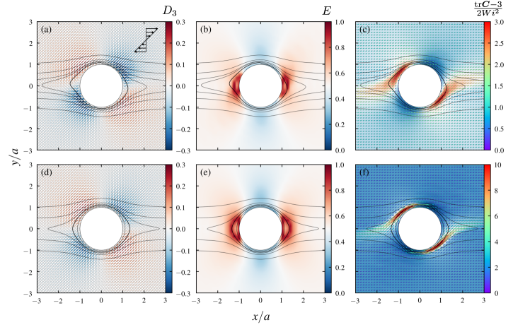
Figure 8: (Color online) Distributions of physical quantities at $\beta=0.5$, $0.99$ and $Wi=2$. The top row panels (a)-(c) and bottom row panels (d)-(f) indicate the results at $\beta=0.5$ and $0.99$, respectively. (a)(d) ellipsoid from strain rate tensor, (b)(e) irrotationality $E$, (c)(f) ellipsoid from conformation tensor. In the panels (a)(d), the elipsoid color is from the out-of-plane eigenvalue $D_{3}$. In the panels (c)(f), the background contour indicates the normalized polymer shear stress as in Fig. 4(c)(d), and the ellipsoid color indicates normalized polymer stretch $(\mathrm{tr}\bm{C}-3)/(2Wi^{2})$, which coincides with unity in an Oldroyd-B fluid without particles under simple shear flow. The bold streamline shows the line that pass through the maximum polymer shear stress.

III.5 Flow and conformation around a particle

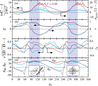
Figure 9: Spatial variations of several fields along the streamlines that pass through the maximum polymer shear stress at $Wi=2$ shown with the bold line in Fig. 8. The horizontal axis $\phi_{s}$ specifies the angle from the velocity gradient direction ($y$ axis), depicted in the right inset in the panel (d). The red lines represent $\beta=0.99$; blue lines represent $\beta=0.5$. With the exception of (d), the solid lines are for left axis, and dashed lines are for right axis. (a) left: $(\mathrm{tr}\bm{C}-3)/(2Wi^{2})$, right: $\sigma_{p,xy}/(1-\beta)$. Spikes at $\beta=0.99$ are artifacts due to mesh resolution. (b) left: $E$, right: $s=3\sqrt{6}\det\bm{D}/(\bm{D}:\bm{D})^{(3/2)}\in[-1,1]$, which indicates the 3D flow patterns Nakayama2016 : $s<0$ for biaxial elongation, $s=0$ for planar shear, and $s>0$ for uniaxial elongation. (c) left: $\sqrt{2\bm{D}:\bm{D}}-1$, right: $\dot{\varepsilon}_{p}$ (d) $\theta_{\bm{D}},\theta_{\bm{C}}$, the angles of $\bm{D},\bm{C}$ ellipsoids from the shear direction (left inset in (d)).

Here, we focus on the relationship between polymer stress and velocity modulation. Figure 7 shows two streamlines on the shear plane at $\beta=0.5$ and $Wi=2$ from the velocity (black line) and the disturbance velocity (blue line), i.e., $\delta\bm{u}=\bm{u}-\bm{u}_{nw}$, where $\bm{u}_{nw}$ is the velocity field in a Newtonian medium at the same $\dot{\gamma}$ and $Re$. Polymer stress induces the anticlockwise disturbance to the velocity near the particle, which corresponds to slowdown of particle rotation speed in viscoelastic media DAvino2008 ; Snijkers2009 ; Snijkers2011 ; Housiadas2011 ; Housiadas2011b . Furthermore, in the recirculation region, the fluid goes away by spiraling out from the particle vicinity to the downstream, thereby forming fore-aft asymmetric streamlines, and such phenomena at finite $Wi$ have been reported in Second-order Fluid Subramanian2007 and Giesekus fluid DAvino2008 ; Housiadas2011 systems. Figure 7 also shows the force density vector $\nabla\cdot\bm{\sigma}_{p}$, exhibiting a correlation between $\nabla\cdot\bm{\sigma}_{p}$ and the disturbance streamlines. In short, the flow disturbance caused by the polymer stress is consistent with the previously reported flow characteristics in viscoelastic suspensions.

Next, flow pattern and conformation around a particle are analyzed. Figure 8 indicates the distributions of physical quantities about flow and polymer conformation fields at $\beta=0.5$ (the top row) and $\beta=0.99$ (the bottom row) and $Wi=2.0$. Figures. 8(a)(d) and 8(c)(f) show the distributions of $\bm{D}$ and $\bm{C}$ with eigen-ellipsoids, respectively. The eigen-ellipsoid for a symmetric tensor is constructed from the three eigenvalues and normalized eigenvectors $(A_{i},\bm{n}_{i})~{}(i=1,2,3)$, where we take $A_{1}>A_{2}$ and $\bm{n}_{3}$ is directed normal to the shear plane. In Figs. 8(a)(d) and 8(c)(f), the ellipsoids are drawn as their major/minor axes are $(1+kA_{1})\bm{n}_{1}$ and $(1+kA_{2})\bm{n}_{2}$, respectively, where $k>0$ is a scaling constant.

Change in flow pattern around a particle is analyzed with $\bm{D}$-ellipsoid in Figs. 8(a)(d) and the irrotationality shown in Figs. 8(b)(e). The $\bm{D}$-ellipsoid with $D_{3}$ indicates the flow patterns at each position, e.g. an elongated ellipsoid with a negative/positive $D_{3}$ indicates uniaxial/biaxial elongational flows. From the upstream to downstream, the flow pattern around the particle varies from biaxial elongation, to planar shear, and then uniaxial elongation. This flow patterns mainly originate from the existence of the particle: at the upstream, flow avoiding the particle creates biaxial elongational flow while converging flow at the downstream creates uniaxial elongational flow. Figures 8(b)(e) display the irrotationality

$$E=\frac{\sqrt{\bm{D}:\bm{D}}}{\sqrt{\bm{D}:\bm{D}}+\sqrt{\bm{\Omega}:\bm{\Omega}^{T}}},$$ (23)

where $\bm{\Omega}=(\nabla\bm{u}-\nabla\bm{u}^{T})/2$ is the vorticity tensor Nakayama2016 . For rigid-body rotation, $E=0$, while $0<E<1$ for the partially rotational flow. Note that the irrotational flow indicated by $E=1$ is a strain-dominated flow; thus, $E$ is conveniently used to identify the strain-dominated flow because $E$ is normalized. The appearance of contour of $E$ is similar to that of the velocity-gradient eigenvalue discriminant Einarsson2018 and to that of the second invariant of the velocity gradient Yang2018 , but the latter quantities are not normalized. In a very recent work by Vázquez-Quesada et al. Vazquez-Quesada2019 , the dimensionless parameter $Q=(\bm{D}:\bm{D}-\bm{\Omega}:\bm{\Omega}^{T})/(\bm{D}:\bm{D}+\bm{\Omega}:\bm{\Omega}^{T})$, which is another definition for irrotationality, shows the similar distributions with those of $E$ in our results. Compared with $E$ in Eq. (23), $Q$ is defined with a squared Frobenius norm and is normalized to $-1\leq Q\leq 1$. Since both $E$ and $Q$ are functions of $\sqrt{\bm{\Omega}:\bm{\Omega}^{T}/\bm{D}:\bm{D}}$, they essentially measure the relative magnitude of $\bm{\Omega}$ to that of $\bm{D}$.

The strain-dominated flow develops near the equator of the particle. This is because the rotational flow in bulk simple shear flow is hindered in front and backside of the particle. In contrast, the half-rotational flow develops near the poles (Figs. 8(b)(e)). This is because, near the poles, the simple shear flow is recovered. At $\beta=0.99$, $\bm{D}$-ellipsoids and $E$ around the particle are symmetrically distributed (Figs. 8(d)(e)). By contrast, at $\beta=0.5$, these distributions are distorted corresponding to the flow modulation (Figs. 8(a)(b)).

Change in polymer conformation around a particle is analyzed with $\bm{C}$-ellipsoid in Figs. 8(c)(f). The shape and orientation of a $\bm{C}$-ellipsoid correspond to the ensemble-averaged stretch and orientation of dumbbell molecules at each position. In the region with high polymer shear stress, we observe that the $\bm{C}$-ellipsoid is highly deformed and oriented by $45^{\circ}$ to the shear flow direction. At $\beta=0.99$, the ellipsoids at such region are more stretched than those at $\beta=0.5$ (Fig. 8(f)). This local high stretching of $\bm{C}$-ellipsoids corresponds to the polymer stress concentration observed in Fig. 4(d).

The development of polymer stress near the particle is determined by the variation of $\bm{C}$-ellipsoids, which is distorted and rotated along the recirculation streamline. Figure 9 shows the variations of fields along the recirculation streamline that pass through the maximum polymer shear stress at $Wi=2$ (bold streamlines in Fig. 8). Along the recirculation, the conformation is periodically stretched and relaxed (left axis in Fig. 9(a)). The normalized polymer stretch is proportional to the polymer dissipation as

$$\Phi_{p}=\frac{\mathrm{tr}\bm{\sigma}_{p}}{2Wi}=(1-\beta)\frac{\mathrm{tr}\bm{C}-3}{2Wi^{2}}.$$ (24)

The shear component of the polymer stress (right axis in Fig. 9(a)) depends on both the polymer stretch and the orientation of $\bm{C}$ as denoted by $\theta_{\bm{C}}$ (Fig 9(d)). In Fig 9, the upstream regions of the maxima in $\mathrm{tr}\bm{C}$ $(\phi_{s}\in[80^{\circ},130^{\circ}],[260^{\circ},310^{\circ}])$ are colored, at which polymer stretching progresses. Prior to entering these regions, $E$ (left axis in Fig. 9(b)) grows immediately, indicating that the flow becomes more strain-dominated. Note that $\theta_{\bm{C}}$ does not change significantly where $E$ is high. Correspondingly, $\theta_{\bm{C}}$ abruptly approaches $\theta_{\bm{D}}$, the primary direction of $\bm{D}$ (Fig. 9(d)), under uniaxial elongational flow (right axis in Fig. 9(b)). At $\beta=0.99$, the primary directions of $\bm{D}$ and $\bm{C}$ are nearly aligned, i.e., $\theta_{\bm{C}}\approx\theta_{\bm{D}}$, in the shaded regions. As a result, the flow pattern in the shaded regions in Fig. 9 strongly facilitates the polymer stretch with a certain level of strain rate $\sqrt{2\bm{D}:\bm{D}}$ (left axis in Fig. 9(c)) under biaxial elongational flow (right axis in Fig. 9(b)). Approaching the poles, $E$ decreases; thus the polymers are subject to rotation, which causes a gradual change in $\theta_{\bm{C}}$ and a discrepancy between $\theta_{\bm{C}}$ and $\theta_{\bm{D}}$. Due to this misalignment, $\mathrm{tr}\bm{C}$ and the polymer shear stress relax regardless of the finite strain rate.

These two effects of strain rate and orientation alignment on the polymer stretch are combinedly reflected in the effective molecular extension rate

$$\dot{\varepsilon}_{p}=\bm{n}_{1}\bm{n}_{1}:\bm{D},$$ (25)

which is the elongation rate in the primary direction of conformation $\bm{n}_{1}$ Pasquali2002 . When the alignment is high, $\dot{\varepsilon}_{p}$ takes a positive value (right axis in Fig. 9(c)), thereby indicating the stretch of the polymers. In contrast, when the orientations are rather perpendicular, $\dot{\varepsilon}_{p}$ takes a negative value, which indicates the compression of the polymers. In the shaded regions in Fig. 9, polymers are exposed to strong stretching. At $\beta=0.99$, $\dot{\epsilon}_{p}\approx 0.5$. In this situation, the local extension rate normalized by $\lambda$, $Wi\dot{\epsilon}_{p}=1.0$, is twice larger than the strain-hardening threshold of the Oldroyd-B fluid $Wi\dot{\epsilon}_{p}=0.5$, above which rate, a dumbbell molecule in the Oldroyd-B fluid is subject to unbounded extension Bird1987 . This extensional characteristics of the Oldroyd-B fluid is supposed to facilitate the polymer stretch in the shaded region in Fig. 9(a) and the development of localized large polymer shear stress in Fig. 8(f). On the other hand, at $\beta=0.5$, $Wi\dot{\varepsilon}_{p}$ in the shaded region is reduced to about $0.6$, which reflects the reduced alignment and strain rate for $\beta=0.5$. This reduction of the local effective extension rate at $\beta=0.5$ results in the weak growth of polymer stretch (Fig. 9(a)). This $\beta$-dependence originates from the modulation of the flow at small $\beta$, which causes the changes in the flow pattern along the recirculation streamlines and in the conformation kinetics.

This analysis explains the polymer stress development near the particle at $\beta=0.99$ and suppression of the stress development at $\beta=0.50$: i.e., the underlying mechanism of the change in the shear-thickening of polymer stress by $\beta$ values, which has not been addressed in the previous studies. Furthermore, our results suggest that at larger $\beta$ conditions, the $Wi$-dependence of shear-thickening of viscoelastic suspensions is more sensitively affected by the elongational property of the viscoelastic media as pointed out by Yang and Shaqfeh Yang2018 . Conversely, at small $\beta$ conditions, the flow modulation by large polymer stress decreases the local effective extension rate and consequently weakens the $Wi$-dependence of shear-thickening of viscoelastic suspensions.

IV Conclusions

In this study, we examined unclear effects of fluid elasticity on shear-thickening in the suspension in an Oldroyd-B medium with a newly developed direct numerical simulation based on the SPM Nakayama2005 ; Nakayama2008 ; Molina2016 . As indicated in the elastic parameter $S_{R}=(1-\beta)Wi$, fluid elasticity is enhanced with both $Wi$ and $1-\beta$. Our results demonstrate that coupling between the polymer stress and flow is enhanced with increasing $1-\beta$, which results in modulation of the velocity and the suppression of the increase in the normalized polymer stress proximity of the particle. This change in polymer stress development leads to the weakening of the $Wi$-dependence of shear-thickening in average polymer stress while the stresslet does not change significantly, resulting in non-trivial weakening of the $Wi$-dependence of the total suspension viscometric functions. Our results suggest that this counteracting effect of fluid elasticity with $1-\beta$ and $Wi$ is critically important for suspension in real moderate or strongly viscoelastic fluids and hydrodynamic interactions. Indeed, the weakening of shear-thickening in large $Wi$ region is observed experimentally Zarraga2001 ; Scirocco2005 ; Tanner2013 , which is consistent with our results.

These results represent a step forward for understanding the role of coupling between viscoelastic response and flow in shear-thickening in viscoelastic suspensions. Previous experimental studies indicate the weakening of shear-thickening in large $Wi$ region Zarraga2001 ; Scirocco2005 ; Tanner2013 , followed by a numerical study to observe the change in $Wi$ dependence of the shear-thickening in average polymer stress at $\beta=0.68$ Yang2018 ; however, how the viscoelastic stress-flow coupling at a finite $1-\beta$ alter the shear-thickening was not explored. In this study, analysis of flow pattern and conformation kinetics around the particle at a finite $1-\beta$ in addition to $\beta=0.99$ clarified the underlying physics of the change in the bulk suspension rheology by the coupling between the polymer stress and flow, which has not been addressed in the previous studies.

Note that shear-thickening of a suspension can also be affected by other factors in constitutive modeling of the medium, such as shear thinning, and the extensibility of polymers Yang2018 . Unconstrained extensibility of polymer in Oldroyd-B fluid is most pronounced when the polymer stress is passive to flow at $\beta\to 1$. Oldroyd-B fluid used in this study is too simple to capture all the aspects of real viscoelastic fluids and thus our results should be carefully interpreted and validated compared with experimental results in the future. Nonetheless, the coupling between the polymer stress and the flow observed in this study should be generally relevant regardless of the individual characteristics of different constitutive models. The detail analysis of flow and conformation in this study would give general insights into microscopic behavior of suspending polymers in real viscoelastic fluids.

References

- (1) I. E. Zarraga, D. A. Hill, and D. T. Leighton, J. Rheol. 45, 1065 (2001).
- (2) R. Scirocco, J. Vermant, and J. Mewis, J. Rheol. 49, 551 (2005).
- (3) S.-C. Dai, F. Qi, and R. I. Tanner, J. Rheol. 58, 183 (2014).
- (4) D. L. Koch, E. F. Lee, and I. Mustafa, Phys. Rev. Fluids 1, 013301 (2016).
- (5) M. Yang, S. Krishnan, and E. S. Shaqfeh, J. Non-Newtonian Fluid Mech. 233, 181 (2016).
- (6) J. Einarsson, M. Yang, and E. S. G. Shaqfeh, Phys. Rev. Fluids 3, 013301 (2018).
- (7) M. Yang and E. S. G. Shaqfeh, J. Rheol. 62, 1363 (2018).
- (8) M. Yang and E. S. G. Shaqfeh, J. Rheol. 62, 1379 (2018).
- (9) R. B. Bird, C. F. Curtiss, R. C. Armstrong, and O. Hassager, Dynamics of Polymeric Liquids, Volume 2: Kinetic Theory (Wiley, ADDRESS, 1987).
- (10) D. F. James, Annu. Rev. Fluid Mech. 41, 129 (2009).
- (11) R. Scirocco, J. Vermant, and J. Mewis, J. Non-Newtonian Fluid Mech. 117, 183 (2004).
- (12) D. Won and C. Kim, J. Non-Newtonian Fluid Mech. 117, 141 (2004).
- (13) R. Pasquino, F. Snijkers, N. Grizzuti, and J. Vermant, Rheol. Acta 49, 993 (2010).
- (14) W. R. Hwang and M. A. Hulsen, Macromol. Mater. Eng. 296, 321 (2011).
- (15) I. S. Santos de Oliveira et al., J. Chem. Phys. 135, 104902 (2011).
- (16) I. S. Santos de Oliveira, W. K. den Otter, and W. J. Briels, J. Chem. Phys. 137, 204908 (2012).
- (17) Y. J. Choi and M. A. Hulsen, J. Non-Newtonian Fluid Mech. 175-176, 89 (2012).
- (18) R. Pasquino, D. Panariello, and N. Grizzuti, J. Colloid Interface Sci. 394, 49 (2013).
- (19) S. Van Loon, J. Fransaer, C. Clasen, and J. Vermant, J. Rheol. 58, 237 (2014).
- (20) R. Pasquino et al., J. Non-Newtonian Fluid Mech. 203, 1 (2014).
- (21) N. Jaensson, M. Hulsen, and P. Anderson, J. Non-Newtonian Fluid Mech. 235, 125 (2016).
- (22) M. Ahamadi and O. Harlen, J. Comput. Phys. 227, 7543 (2008).
- (23) M. Ahamadi and O. Harlen, J. Non-Newtonian Fluid Mech. 165, 281 (2010).
- (24) Y. J. Choi, M. A. Hulsen, and H. E. Meijer, J. Non-Newtonian Fluid Mech. 165, 607 (2010).
- (25) N. Jaensson, M. Hulsen, and P. Anderson, J. Non-Newtonian Fluid Mech. 225, 70 (2015).
- (26) W. R. Hwang, M. A. Hulsen, and H. E. Meijer, J. Non-Newtonian Fluid Mech. 121, 15 (2004).
- (27) G. D’Avino, F. Greco, M. A. Hulsen, and P. L. Maffettone, J. Rheol. 57, 813 (2013).
- (28) A. Vázquez-Quesada and M. Ellero, Phys. Fluids 29, 121609 (2017).
- (29) S. Krishnan, E. S. Shaqfeh, and G. Iaccarino, J. Comput. Phys. 338, 313 (2017).
- (30) A. Vázquez-Quesada, P. Español, R. I. Tanner, and M. Ellero, J. Fluid Mech. 880, 1070 (2019).
- (31) Y. Nakayama and R. Yamamoto, Phys. Rev. E 71, 036707 (2005).
- (32) Y. Nakayama, K. Kim, and R. Yamamoto, Eur. Phys. J. E 26, 361 (2008).
- (33) T. Iwashita and R. Yamamoto, Phys. Rev. E 80, 061402 (2009).
- (34) H. Kobayashi and R. Yamamoto, J. Chem. Phys. 134, 064110 (2011).
- (35) J. J. Molina et al., J. Fluid Mech. 792, 590 (2016).
- (36) T. Iwashita, T. Kumagai, and R. Yamamoto, Eur. Phys. J. E 32, 357 (2010).
- (37) Y. Matsuoka, T. Fukasawa, K. Higashitani, and R. Yamamoto, Phys. Rev. E 86, 051403 (2012).
- (38) K. Kim, Y. Nakayama, and R. Yamamoto, Phys. Rev. Lett. 96, 208302 (2006).
- (39) X. Luo, A. Beskok, and G. E. Karniadakis, J. Comput. Phys. 229, 3828 (2010).
- (40) J. J. Molina, Y. Nakayama, and R. Yamamoto, Soft Matter 9, 4923 (2013).
- (41) Y. K. Lee and K. H. Ahn, J. Non-Newtonian Fluid Mech. 244, 75 (2017).
- (42) H. Luo and T. R. Bewley, J. Comput. Phys. 199, 355 (2004).
- (43) D. Venturi, J. Phys. A Math. Theor. 42, 125203 (2009).
- (44) D. R. Mikulencak and J. F. Morris, J. Fluid Mech. 520, 215 (2004).
- (45) H. Haddadi and J. F. Morris, J. Fluid Mech. 749, 431 (2014).
- (46) C.-J. Lin, J. H. Peery, and W. R. Schowalter, J. Fluid Mech. 44, 1 (1970).
- (47) D. L. Koch and G. Subramanian, J. Non-Newtonian Fluid Mech. 138, 87 (2006).
- (48) F. Greco, G. D’Avino, and P. Maffettone, J. Non-Newtonian Fluid Mech. 147, 1 (2007).
- (49) Y. Nakayama, T. Kajiwara, and T. Masaki, AIChE J. 62, 2563 (2016).
- (50) G. D’Avino et al., J. Rheol. 52, 1331 (2008).
- (51) F. Snijkers et al., J. Rheol. 53, 459 (2009).
- (52) F. Snijkers et al., J. Non-Newtonian Fluid Mech. 166, 363 (2011).
- (53) K. D. Housiadas and R. I. Tanner, Phys. Fluids 23, 083101 (2011).
- (54) K. D. Housiadas and R. I. Tanner, Phys. Fluids 23, 051702 (2011).
- (55) G. Subramanian and D. L. Koch, J. Non-Newtonian Fluid Mech. 144, 49 (2007).
- (56) M. Pasquali and L. Scriven, J. Non-Newtonian Fluid Mech. 108, 363 (2002).