Analytical solutions of the cylindrical bending problem for the relaxed micromorphic continuum and other generalized continua (including full derivations)
Abstract
We consider the cylindrical bending problem for an infinite plate as modelled with a family of generalized continuum models, including the micromorphic approach. The models allow to describe length scale effects in the sense that thinner specimens are comparatively stiffer. We provide the analytical solution for each case and exhibit the predicted bending stiffness. The relaxed micromorphic continuum shows bounded bending stiffness for arbitrary thin specimens, while classical micromorphic continuum or gradient elasticity as well as Cosserat models [37] exhibit unphysical unbounded bending stiffness for arbitrary thin specimens. This finding highlights the advantage of using the relaxed micromorphic model, which has a definite limit stiffness for small samples and which aids in identifying the relevant material parameters.
Dedicated to Holm Altenbach on the occasion of his 65th birthday.
Keywords: generalized continua, cylindrical bending, bending stiffness, characteristic length, size-effect, micromorphic continuum, Cosserat continuum, couple stress model, gradient elasticity, micropolar, relaxed micromorphic model, micro-stretch model, micro-strain model, micro-void model, bounded stiffness.
1 Introduction of the cylindrical bending problem
The classical Cauchy-Boltzmann theory of continuum mechanics comes to its limits when the wavelengths of deformation fields become comparable to characteristic microstructural length scales of a material, and therefore generalized continuum theories are necessary in this regime. Micromorphic continuum theories are established today for this purpose due to their direct connection to concepts of classical continuum mechanics and their relatively simple numerical implementation in existing finite element codes. The micromorphic theory contains other approaches like the Cosserat continuum [36, 24, 22], couple stress continuum [15, 28], microstretch continuum, micro-void continuum, the microstrain continuum, the relaxed micromorphic continuum or the strain-gradient theory as special cases [10], among others. An overview can be found in [11, 12]. In the very most cases, any of these subclasses is favoured over the general micromorphic theory since the latter requires a large number of constitutive parameters, namely already 18 for isotropic linear-elastic material. Even more, the effect of most of these parameters on measurable quantities is still rather unclear.
An important milestone was set by Gauthier and Jahsman [14], who derived analytical solutions for bending and torsion of a linear isotropic Cosserat continuum. The gradients under bending and torsion problems activate the non-classical terms, which is why the respective non-classical parameters affect the observable stiffness. Further studies for bending of a linear isotropic Cosserat continuum have been carried out by Altenbach [1, 2]. These solutions have been used in many works to identify the constitutive parameters from real or virtual experiments, e.g. in [14, 46, 23, 45, 41, 44] or they could be a useful tool to reduce the computational load in numerical identification or homogenization schemes, e.g. in [3, 5, 6, 41, 47, 39].
However, certain effects at edges or the dispersion of longitudinal waves could not be explained by the Cosserat theory [27], but more general micromorphic theories are required. The authors in [7] provided the bending solution for the micro-void continuum. However, this theory cannot explain experimentally observed size effects in torsion or dispersion of shear waves. De Cicco and Nappa [9] solved the bending and torsion problem for the microstretch continuum analytically. Further closed-form solutions of the bending and torsion problems have been found for sub-classes of the micromorphic continuum and certain geometries [20, 21, 18, 27, 25, 38, 43]. However, to the best of the authors’ knowledge, no solution is known for the general micromorphic continuum with an unconstrained second-order tensor of microdeformation as kinematic degree of freedom.
The scope of the present paper is to derive and discuss the solution for cylindrical bending for such a general micromorphic continuum and several of its sub-classes, notably the relaxed micromorphic model. A similar investigation with respect to the simple shear problem has been undertaken in [40].
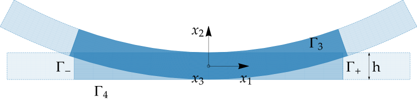
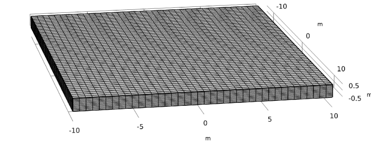
The solid studied here has a finite thickness along the direction while it is infinite in the directions and . Our aim is to describe a state of uniform cylindrical bending in the infinite plate for various models of generalized elasticity. The bending of a plate can be thought of as a result of applying couples at the lateral faces of a suitable large portion of it.
1.1 Notation
For vectors , we consider the scalar product , the (squared) norm and the dyadic product . Similarly, for tensors with Cartesian coordinates and , we define the scalar product and the (squared) Frobenius-norm . Moreover, denotes the transposition of the matrix , which decomposes orthogonally into the symmetric part and the skew-symmetric part . The Lie-Algebra of skew-symmetric matrices is denoted by . The identity matrix is denoted by , so that the trace of a matrix is given by . Using the bijection we have
| (1) |
where denotes the standard cross product in . The inverse is denoted by Anti: . The gradient and the curl for a vector field are defined as
| (2) |
Moreover, we introduce the Curl and the Div operators of the matrix as
| (3) |
The cross product between a second order tensor and a vector is defined as follow
| (4) |
where , , and is the Levi-Civita tensor.
2 Cylindrical bending for the isotropic Cauchy continuum
For comparison we start with the well known classical case.
The expression of the strain energy for an isotropic linear elastic Cauchy continuum is
111
Here are reported the macroscopic 3D Poisson’s ratio , the Young modulus
, and the bulk modulus .
| (5) |
where and are the two classical Lamé constants, and is the bulk modulus. Consequently, the equilibrium equations without body forces are
| (6) |
where is the symmetric Cauchy-stress tensor and is the symmetric strain tensor. The boundary conditions at the upper and lower surface (free surface) are the traction-free forces conditions
| (7) |
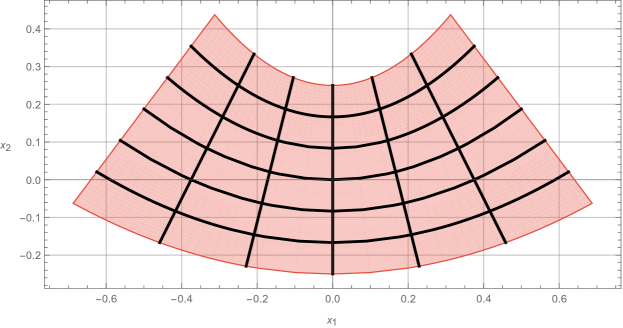
where the expression of is in eq.(6)2 and is the unit vector aligned to the -direction. We are interested in describing a state of uniform curvature of the infinite plate. According to the reference system shown in Fig. 1, the ansatz for the displacement field is
| (8) |
Therein, refers to the deflection of the neutral axis and denotes the lateral contraction. The gradient of the displacement field and its symmetric part (the strain tensor) result to be
| (9) |
It is highlighted that the gradient of eq.(9)1 has a symmetric part which has only diagonal components as it can be seen in eq.(9)2. The equilibrium equations in terms of the ansatz eq.(8) are
| (10) |
Equation.(10)2 requires both and to be a quadratic function in and , respectively, and this already satisfies eq.(10)1:
| (11) |
It is important to highlight that the solution eq.(11) depends on the elastic parameters of the material. In addition, we can further simplify the solution eq.(11) by setting , and since they represent rigid body motions (the first two a rigid translation, while the third one a rigid rotation).
The boundary conditions eq.(7) on the upper and lower surface (stress free surfaces, no tractions), require that . Appling these simplifications while substituting the solution eq.(11) in eq.(8), the displacement field results to be (with ) [17]
| (12) |
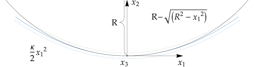
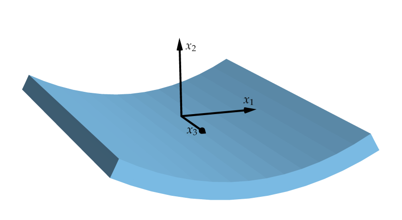
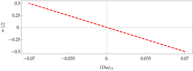
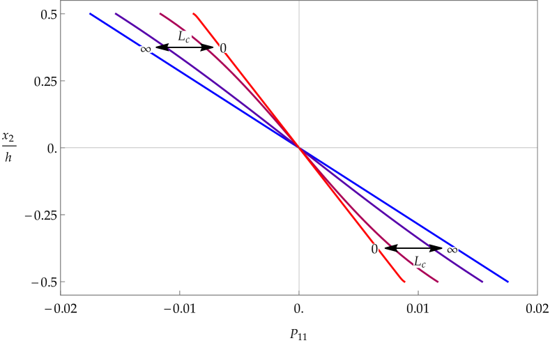
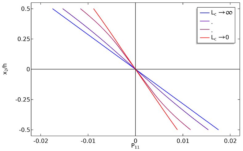
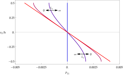
Thus, the middle plane of the infinite plate is bent to a cylindrical surface (see Fig. 1) which is approximated by the parabolic cylinder . Since the displacement field solution depends on the elastic coefficients of the material, two extreme cases are shown in the following Fig. 2 with a plot of across the thickness .
The desired bending moment about the -axis and energy (per unit area dd) expressions are
| (13) | ||||
where is the plane stress first Lamé parameter, is the moment of inertia for a unit thickness, is the curvature, and the quantity
| (14) |
is the classical cylindrical bending stiffness for a plate (flexural rigidity). 222 Note that under the plane stress hypothesis the first Lamé parameter become , while the shear modulus , the Young modulus , and the Poisson’s ratio do not change. It is also reported here the more used bending stiffness expression . It is also highlighted that
| (15) |
Here and in the remainder of this work, the elastic coefficients are expressed in [MPa], the coefficients are dimensionless, the lengths and the thickness in meter [m], the curvature in [1/m].
3 Classical Mindlin-Eringen formulation
The classical micromorphic model couples the displacement with an independent affine field , called the microdistortion. Even in the isotropic case the model has 18 parameters (among them 11 for the curvature) and the elastic energy can be represented as
| (16) | ||||
where is the symmetric part of the gradient of the displacement field, is the difference between the gradient of the displacement field and the microdistortion tensor, and is the full gradient of the microdistortion and is a sixth order tensor.
A general solution of the cylindrical bending problem for the isotropic micromorphic model is not yet known but it could be found by the present ansatz without any fundamental problem, only the formulas get extremely long and complicated. Therefore, we consider the following simplified energy
| (17) | ||||
which is a special case of eq. (16), by setting the values of the elastic parameters as follows (see [32] and Appendix G for the full derivation for the curvature part)
| (18) | ||||
Thus, with this choice of parameters, the former energy can be expressed as
| (19) | ||||
which coincides, apart from the curvature term, with the energy from the relaxed micromorphic model treated in the next paragraph. Note again carefully that the chosen curvature expression is still isotropic [30] but does not represent the most general isotropic curvature expression in this model.
4 Cylindrical bending for the isotropic relaxed micromorphic model
The expression of the strain energy for the isotropic relaxed micromorphic continuum is:
333
Are here reported the 3D Poisson’s ratio , the 3D Young modulus
, and the micro and the meso expression of the Poisson’s ratio in plane stress and the , respectively.
| (20) | ||||
where and are the material parameters related to the meso-scale, and are the parameters related to the micro-scale, is the Cosserat couple modulus, is the characteristic length, and , , and are the three general isotropic curvature parameters. The curvature expression is the most general isotropic one in terms of a dependence on the second order tensor and can be obtained by setting the values of the elastic parameters of the classical micromorphic model eq.(16) as follows (see Appendix G for the full derivation)
| (21) | ||||
The most simple isotropic curvature term corresponds to and would therefore be given by , , Due to [26] the model is well-posed even for and if . The equilibrium equations without body forces are
| (22) | ||||
The boundary conditions at the upper and lower surface (free surface) are
| (23) | ||||
where the expression of and are in eq.(22), is the unit vector aligned to the -direction, is the Levi-Civita tensor, and is the generalized second order moment tensor. The generalised traction vector is and the generalized double traction tensor is .
According with the reference system shown in Fig. 1, the ansatz for the displacement field and the microdistortion is
| (24) |
while the gradient of the displacement field results to be
| (25) |
We supply as well the homogenization relations between the macro-parameters and the meso- (with index ) and micro-parameters [8, 35, 33]
| (26) |
4.1 One curvature parameter and zero Poisson’s ratios
Substituting the ansatz in the following simplified equilibrium eq.(27) where and , results in the simplified curvature and
| (27) | ||||
where the generalized moment tensor is . The equilibrium equations (27) then are
| (28) | |||
It is clear that, in order to satisfy eq.(28)3 and eq.(28)4 either or ; we choose the latter option, which implies that the skew-symmetric part of the gradient of the displacement eq.(25) is the same as the skew-symmetric part of the microdistortion eq.(24)2. This also implies that the Cosserat couple modulus does not play a role any more. Consequently, the solution of eq.(28) is
| (29) | ||||
The boundary conditions eq.(23) on the upper and lower surfaces allow to evaluate the constants as shown in the following 444 .
| (30) |
Finally, the displacement and microdistortion components result in
| (31) | ||||
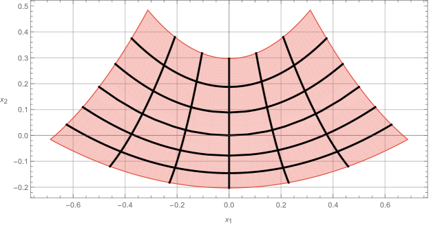
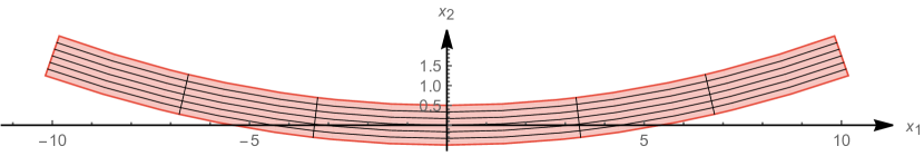
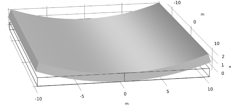
It is underlined that for this specific case and turn out to be equal to zero. In Fig. 3 we show the deformed shape due to the displacement field solution
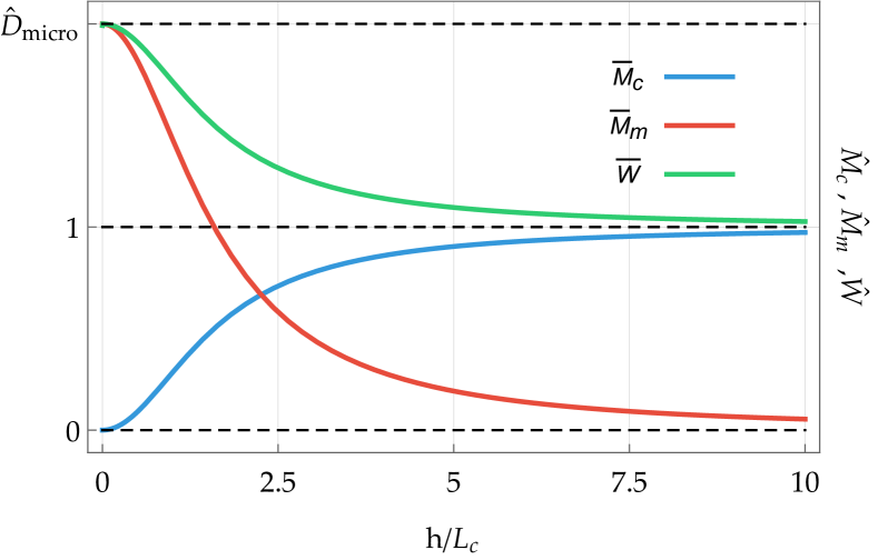
The classical bending moment, the higher-order bending moment, and energy (per unit area dd) expressions are reported next in the following eq.(32)
| (32) | ||||
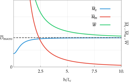
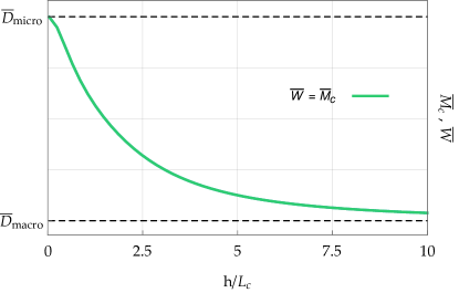
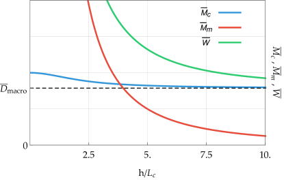
The plot of the bending moments and the strain energy divided by and , respectively, while changing is shown in Fig. 4(a).

As in the classical Cauchy elastic case, we have
| (33) |
4.1.1 Remarks on the boundary conditions: consistent coupling
If a finite slice is cut along the -direction at distance from the origin, a finite solid in the plane is obtained. The kinematic boundary conditions that arise on the cut surfaces and (see Fig. 1) for this solution are
| (34) |
Moreover, it holds that at , which implies that for zero Poisson’s ratios , the consistent coupling condition
| (35) |
at the lateral boundary and is exactly verified. This means that in this exceptional case we could start alternatively with a finite domain boundary value problem and describe the bending condition according to eq.(34)1 and in addition require at the lateral boundary and , giving the ansatz eq.(24), since the solution of the problem is unique [35].
The static boundary conditions that arise on the cut surfaces and (see Fig. 1) are
| (36) | ||||
where and are the only components different from zero. It is also highlighted that the compatibility condition expressed by eq.(36)2 is satisfied. The boundary conditions eq.(23) on the upper and lower surface in addition to eq.(34) or eq.(36) (the choice is up to the reader) on the left and right surface are enough to retrieve the full solution eq.(31).
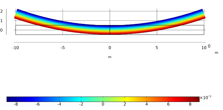
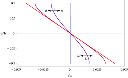
The plot of obtained analytically and numerically (via COMSOL) while changing is shown in Fig. 5(a) and Fig. 5(b), respectively: the two give correctly the exact same results.
In Fig. 6 is shown the deformed shape obtained thanks to simulations done via COMSOL.
4.1.2 Limit cases
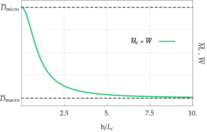
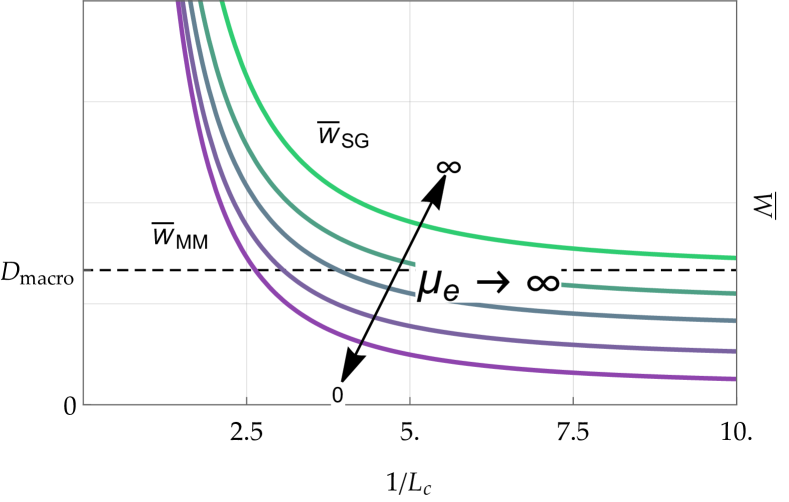
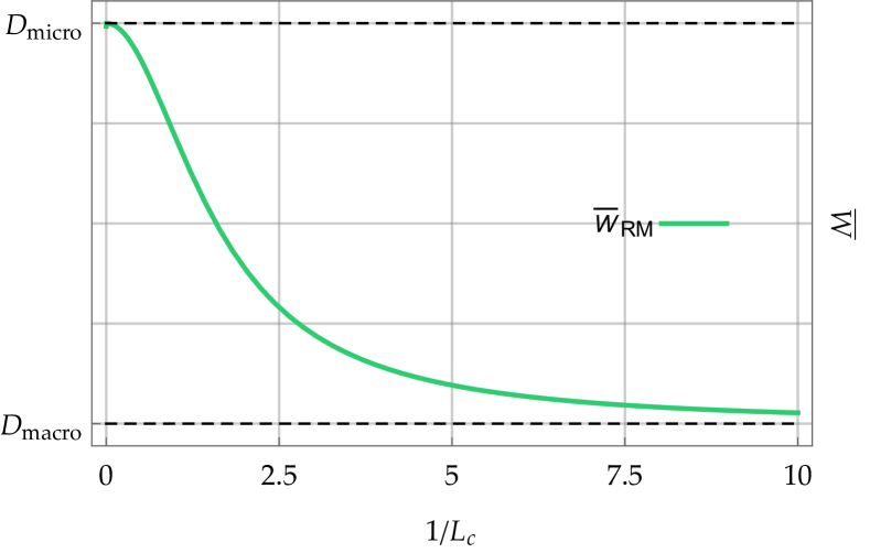
We consider in the following the two limit cases: first corresponds to arbitrary thick specimens, while secondly corresponds conceptually to arbitrary thin specimens. We see that in the relaxed micromorphic model, this corresponds unequivocally to the stiffness and , respectively, since
| (37) | ||||
4.2 One curvature parameter and arbitrary Poisson’s ratios and
Substituting the ansatz in the following simplified equilibrium eq.(38) where
| (38) | ||||
where the generalized moment tensor is . The equilibrium equation (38) are
| (39) | ||||
In order to satisfy eq.(39)3 and eq.(39)4 either or ; we have chosen the latter option, which implies that the skew-symmetric part of the gradient of the displacement eq.(25) is the same as the skew-symmetric part of the microdistortion eq.(24)2. This also implies that the Cosserat couple modulus does not play a role any more.
From eq.(39)1 it is possible to evaluate and consequently
| (40) | ||||
By substituting back eq.(40) in eq.(39), we can evaluate and its derivatives from equation eq.(39)5
| (41) | ||||
After substituting eq.(41) in eq.(39) the following two second order ordinary differential equations in and are retrieved
| (42) | |||
where
| (43) | ||||
These additional relations between the parameters are satisfied
| (44) | ||||
where and are the plane stress bulk moduli expressions at the micro-and meso-scale, respectively. Finally, the solution of eq.(42) is
| (45) | ||||
Given boundary conditions eq.(23) for this case, the integration constants reduce to
| (46) | ||||
The classical bending moment, the higher-order bending moment, and energy (per unit area dd) expressions are
| , | ||||
| , | (47) | |||
| (48) | ||||
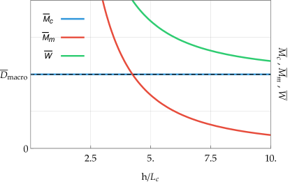
Again, The plot of the bending moments and the strain energy divided by and , respectively, while changing is shown in Fig. 7.

4.2.1 Limit cases
| (49) | ||||
4.3 Full isotropic curvature and zero Poisson’s ratios
The expression of the strain energy for the isotropic relaxed micromorphic continuum is
| (50) | ||||
while the equilibrium equations without body forces are
| (51) | ||||
Substituting the ansatz eq.(24) in eq.(51) the equilibrium equations result to be
| (52) | |||
It is clear that in order to satisfy eq.(52)3 and eq.(52)4 either or ; it has been chosen the latter option, which implies that the skew-symmetric part of the gradient of the displacement eq.(25) is the same as the skew-symmetric part of the microdistortion eq.(24)2. This also implies that the Cosserat couple modulus does not play a role any more.
From eq.(52)1 it is possible to evaluate and consequently
| (53) |
By substituting back eq.(53) in eq.(52), we can evaluate and its derivatives from equation eq.(52)5
| (54) |
After substituting eq.(54) in eq.(52) the following two coupled second order ordinary differential equations in and are obtained
| (55) | |||
Finally, the solution of eq.(55) is
| (56) | ||||
Given boundary conditions eq.(23) for this case, the integration constants reduce to
| (57) | ||||
The classical bending moment, the higher-order bending moment, and energy (per unit area dd) expressions are
| (58) | ||||
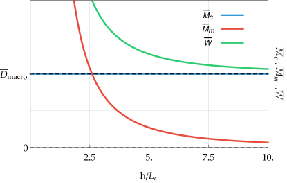
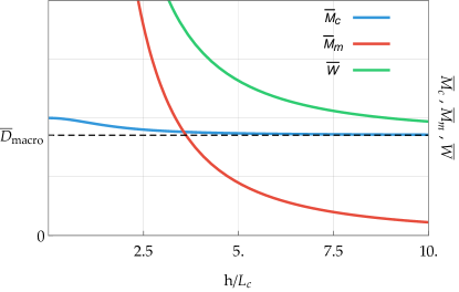
Again, The plot of the bending moments and the strain energy divided by and , respectively, while changing is shown in Fig. 8.
4.3.1 Limit cases
| (59) | ||||
4.4 Full isotropic curvature and arbitrary Poisson’s ratios and
Finally, we are prepared to treat the most general case of an isotropic, linear-elastic relaxed micromorphic continuum.. The expression of the strain energy for the isotropic relaxed micromorphic continuum is:
| (60) | ||||
while the equilibrium equations without body forces are
| (61) | ||||
Substituting the ansatz eq.(24) in eq.(61) the equilibrium equations are
| (62) | ||||
In order to satisfy eq.(62)3 and eq.(62)4 either or ; we have chosen the latter option, which implies that the skew-symmetric part of the gradient of the displacement eq.(25) is the same as the skew-symmetric part of the microdistortion eq.(24)2. This also implies that the Cosserat couple modulus does not play a role any more.
From eq.(62)1 it is possible to evaluate and consequently
| (63) | ||||
By substituting back eq.(63) in eq.(62), we can evaluate and its derivatives from equation eq.(62)5
| (64) | ||||
After substituting eq.(64) in eq.(62) the following two coupled second order ordinary differential equations in and are retrieved
| (65) | |||
Finally the solution of eq.(65) is
| (66) | ||||
Given boundary conditions eq.(23) for this case, the integration constants reduce to
| (67) | ||||
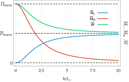
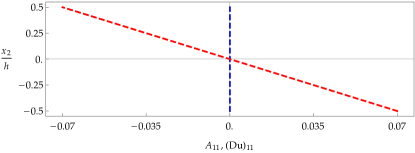
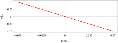
In Fig. 9(a) we present the distribution across the thickness of while varying .
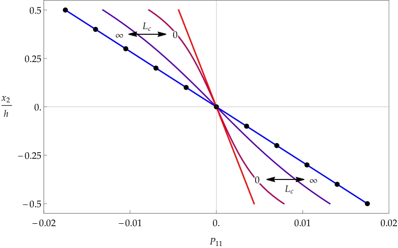

The increase of as is counterintuitive in the first instance, since the stiffness increases as but it can be explained as follow: (i) for it is possible to demonstrate that which justifies the fact that is superimposed to for ; (ii) for it is possible to demonstrate that and it will be anyway always smaller than .
The classical bending moment, the higher-order bending moment, and energy (per unit area dd) expressions are
| (68) | ||||
where
| (69) | ||||
Again, The plot of the bending moments and the strain energy divided by and , respectively, while changing is shown in Fig. 10.

4.4.1 Limit cases
In addition to the two limits we consider here as well since this makes for the transition to the classical Cosserat model.
| (70) |
5 The micro-stretch model in dislocation format
The micro-stretch model in dislocation format [35] can be obtained from the relaxed micromorphic model by letting formally , while . For bounded energy, this constrains , , . Thus the micro-stretch model has 4 additional degrees of freedom. The expression of the strain energy for the isotropic micro-stretch continuum in dislocation format (i.e. with curvature energy only depending on the dislocation density tensor ) can then be written as [35]:
| (71) | ||||
since . The equilibrium equations without body forces are then
| (72) | ||||
The boundary conditions at the upper and lower surface (free surface) are
| (73) | ||||
According with the reference system shown in Fig. 1, the ansatz for the displacement field and the function is
| (80) |
The equilibrium equations (72) then result in 555Where and are the meso- and the micro-scale 3D bulk modulus.
| (81) | |||
since the second equation eq.(72)2 is already satisfied. From eq.(81)1 it is possible to evaluate and consequently as follows
| (82) | ||||
Substituting back the expression of and in (81) it is possible to evaluate from eq.(81)2 and consequently which results in
| (83) | ||||
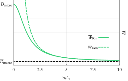
In Fig. 12 we present the distribution across the thickness of while varying .

The classical bending moment, the higher-order bending moment , and energy (per unit area dd) expressions are
| (84) | ||||
One of the two higher-order bending moment is zero and we have . The plot of the non zero bending moments and the strain energy divided by and , respectively, while changing is shown in Fig. 13.
5.0.1 Limit cases
| (85) | ||||||
6 Cylindrical bending for the isotropic Cosserat continuum
The expression of the strain energy for the isotropic Cosserat continuum in dislocation tensor format can be written 666 The equivalent formulation in terms of a rotation vector is given in the appendix.
| (86) | ||||
where . The Cosserat energy can be obtained from the relaxed micromorphic model by letting formally or letting in the micro-stretch model.
It is important to underline that, since and for a plane problem (see Appendix C), the elastic energy ends up to have only one effective curvature parameter
| (87) | ||||
The equilibrium equations without body forces are the following:
| (88) | ||||
The boundary conditions for the upper and lower surface (free surface) are
| (89) | ||||
where the expression of is in eq.(88), is defined the unit vector aligned to the -direction, is the Levi-Civita tensor, and the moment stress tensor . The bending Neumann condition at the upper and lower surface will be derived in Appendix B.
According to the reference system shown in Fig. 1, the ansatz for the displacement field and the micro-rotation is
| (90) |
while the gradient of the displacement field result to be
| (91) |
Substituting the ansatz eq.(90) in eq.(88) the equilibrium equations turn in
| (92) | |||
In order to satisfy eq.(92)2 and eq.(92)3 either or ; we have chosen the latter option, which implies that the skew-symmetric part of the gradient of the displacement eq.(91) is the same as the skew-symmetric part of the micro-rotation eq.(90)2. This also implies that the Cosserat couple modulus does not play a role any more. Consequently, the solution (deprived of the rigid body motion) of eq.(92) is
| (93) |
The boundary conditions eq.(89)1 on the upper and lower surfaces constrain , while the second one eq.(89)2 is identically satisfied. Then, the displacement and micro-rotation fields solution are
| (94) |
The displacement field eq.(94) is the same as the classical one eq. (12). In Fig. 14 we shown the plot of across the thickness.
The classical bending moment, the higher-order bending moment, and energy (per unit area dd) expressions are reported in the following eq.(95).
| (95) | ||||
Finally, there is only one combination of curvature parameters appearing. Inverting the formula gives and this parameter is traditionally called the bending length scale of the Cosserat model (see Appendix D.1). There is no counterpart to this observation in the relaxed micromorphic model or in the micro-stretch model. Again, The plot of the bending moments and the strain energy divided by and , respectively, while changing is shown in Fig. 15.
7 Micro-void model in dislocation tensor format
The expression of the strain energy for the isotropic micro-void continuum with a single curvature parameter in dislocation tensor format (3+1=4 dof’s) can be written as:
| (96) | ||||
Here, describes the additional scalar micro-void degree of freedom. Since , the isotropic curvature reduces to . The equilibrium equations without body forces are 777 Where and are he meso- and the micro-scale 3D bulk modulus.
| (97) | ||||
The boundary conditions at the upper and lower surface (free surface) are
| (98) | ||||
According with the reference system shown in Fig. 1, the ansatz for the displacement field and the function is
| (99) |
The equilibrium equations (97) turn in
| (100) | |||
Form eq.(100)1 it is possible to evaluate and consequently as follows
| (101) | ||||
Substituting back the expression of and in eq.(100) it is possible to evaluate from eq.(100)2 and consequently which implies
| (102) | ||||
In Fig. 16 we show the distribution across the thickness of while varying .

The classical bending moment, the higher-order bending moment, and energy (per unit area dd) expressions are reported in the following eq.(103)
| (103) | ||||
Since the higher-order bending moment is zero and only the plot of energy divided by while changing is shown in Fig. 17.
7.0.1 Limit cases
If (which is the consistent case for the micro-void model) then (see the homogenization formulas eq.(26)) and we obtain
| (104) | ||||
- •
-
•
If , in order for a minimum of the energy to exist, it is required that which means that has to be the gradient of a scalar function , which implies that must be constant. The boundary conditions eq.(98)2 requires to be zero on the upper and lower surface and since must be constant, this is automatically satisfied.
While the micro-void model in dislocation format has bounded stiffness in cylindrical plate bending, the micro-stretch model does not. This may look strange given that the micro-stretch model should be more ”flexible” having more independent degrees of freedom (the additional micro-rotation ). However, the specific coupling with the curvature terms dictate otherwise. This also shows that the micro-void model is not a simple “penalization” of the micro-stretch model.
8 Cylindrical bending for the isotropic couple stress continuum family
The indeterminate couple stress models [34] appear by letting formally the Cosserat couple modulus . This implies the constraint . It is highlighted that this constraint is automatically satisfied given the ansatz eq.(90) and the equilibrium equation’s requirement that (which also implies that the solution is finally independent of the Cosserat couple modulus ), setting the energy for the isotropic Cosserat model equal to the one of the isotropic indeterminate couple stress model.
The indeterminate couple stress elastic energy turns into
| (107) | ||||
Since, however, and
for a plane problem, we are left with
| (108) | ||||
The equilibrium equations without body forces are
| (109) | |||
while the boundary condition on the upper and lower surface are (for more details see [34])
| (110) | ||||
where , is the unit vector aligned to the -direction, and the second order moment stress . The operator Anti is defined as the inverse of axl in the context of eq.(1). The term measures the discontinuity of across the boundary.
According to the reference system shown in Fig. 1, the ansatz for the displacement field and consequently the gradient of the displacement are
| (111) |
Consequently, the solution (deprived of the rigid body motion) of eq.(112) is:
| (113) |
The boundary conditions eq.(110)1 on the upper and lower surfaces constrain , while eq.(110)2 and eq.(110)3 are identically satisfied. Then, the displacement field solution results in
| (114) |
The displacement field eq.(114) is the same as the classical one eq.(12). In Fig. 18 we show the plot of across the thickness:

The classical bending moment, the higher-order bending moment, and energy (per unit area dd) expressions are reported in the following eq.(115)
| (115) | ||||
The result coincides with the Cosserat solution eq.(95). Note that The plot of the bending moments and the strain energy divided by and , respectively, while changing is shown in Fig. 19.

8.1 Cylindrical bending for the isotropic symmetric couple stress continuum
The modified couple stress model [31] consist in choosing , and the (“pseudo”)-consistent couple stress model [16] appears for , . Since due to for a plane problem, the form of the energy remains the same. For the cylindrical bending problem, the higher order Neumann boundary conditions are already identically satisfied for all these models, like for their general case which is the relaxed micromorphic model.
9 Cylindrical bending for the classical isotropic micromorphic continuum without mixed terms
The expression of the strain energy for the reduced isotropic micromorphic continuum without mixed terms (like , etc.) and simplified isotropic curvature can be written as
| (116) | ||||
The meaning of , , and for the third order tensor can be inferred from eq.(116), i.e. we define
| (117) | |||
The equilibrium equations (see the Appendix E) without body forces are the following
| (118) | |||
where is taken component-wise. The boundary conditions (see the Appendix E) at the upper and lower surface (free surface) are
| (119) | ||||
where , , is a second order tensor, and is the ith component of the unit vector (see the Appendix E). According with the reference system shown in Fig. 1, the ansatz for the displacement field and the microdistortion is
| (120) |
Substituting the ansatz eq.(120) in eq.(118) the equilibrium equation are
| (121) | ||||
It is possible to evaluate from eq.(121)1 and then form a linear combination of the remaining equation. After substituting the expressions of and in eq.(121), we are left with two coupled ordinary differential equations of fourth order in and . The solution is again of hyperbolic type and the unknown coefficients are determined by the boundary conditions eq.(119).
In Fig. 20 we show the distribution across the thickness of while varying .
Subsequently, the bending moments and the strain-energy per unit area are computed by
| (122) | |||
where is the scalar ith component of the unit vector , similarly to eq.(119) .
The symbolic expressions are too long to be reported here, but we provide a plot of the bending moments and the strain energy divided by and , respectively, in Fig. 21 for selected parameter sets while changing . Still we have

9.1 Penalized second gradient elasticity
The classical Mindlin-Eringen micromorphic model can also be interpreted as a penalty formulation of second gradient elasticity. Indeed, letting imposes the constraint and the remaining minimization problem is of the type
| (123) |
We consider the stiffness generated for this limit in the simple case and we investigate this specific limit case since it remains analytically treatable.
10 Cylindrical bending for the micro-strain model without mixed terms
The micro-strain model [13, 19] can be obtained from the classical Mindlin-Eringen model by assuming a priori that the microdistortion remains symmetric, .
A bending solution for a particular model of this type has been derived in [18] disregarding of the lateral contraction. This simplification shall be overcome here, whereby we employ a reduced isotropic curvature expression to make the calculations manageable.
Note that the micro-strain model cannot be obtained from the relaxed micromorphic model, although there are certain similarities. The free energy which we consider is given by
| (124) | ||||
The meaning of and for the third order tensor can be inferred from eq.(124), i.e. we define
| (125) |
The chosen 2-parameter curvature expression represents a simplified isotropic curvature (the full isotropic curvature for the micro-strain model still counts 8 parameters [4]). If the chosen curvature energy provides a complete control of .
If we assume that , while , then the model turns formally also into the micro-void model (see Section 7) i.e. . Then the curvature turns into 888 Note that
| (126) | ||||
The equilibrium equations without body forces are the following (see Appendix E)
| (127) | |||
where is taken component-wise. The boundary conditions (see the Appendix E) at the upper and lower surface (free surface) are
| (128) | ||||
where , is a second order tensor and is the scalar ith component of the unit vector (see the Appendix E). According with the reference system shown in Fig. 1, the ansatz for the displacement field and the microdistortion is
| (129) |
Substituting the ansatz eq.(129) in eq.(127) the equilibrium equation results in
| (130) | ||||
It is possible to evaluate from eq.(130)1 and then form a linear combination of the remaining equation. After substituting the expressions of and in eq.(130), we are left with two coupled ordinary differential equations of fourth order in and .
In Fig. 23 we show the distribution across the thickness of while varying .
The classical bending moment, the higher-order bending moment, and energy (per unit area dd) definitions are reported in the following eq.(131)
| (131) | |||
where is the scalar ith component of the unit vector .
Again, the symbolic expressions are lengthy and are thus not reported here in detail. Fig.24 provides a graphical representation of the final result. Since the higher-order bending moment is zero and the following relation holds
| (132) |
only the plot of energy [42] (per unit area dd) while changing is shown in Fig. 24
The energy of the model remains bounded, as for the micro-void model, since for both models the higher-order bending moment are zero, and this does not create a conflict with the boundary condition as .
11 Cylindrical bending for the second gradient continuum
The expression of the most general isotropic strain energy for the second gradient continuum is [29]
| (133) | ||||
where (). The expression we are going to use in the following is a simplified isotropic strain energy with three curvature parameters
| (134) | ||||
The meaning of , , and for the third order tensor can be inferred from eq.(134), i.e. we define
| (135) | |||
The equilibrium equations (see the Appendix F) without body forces are
| (136) | |||
where , is taken component-wise. According with the reference system shown in Fig. 1, the ansatz for the displacement field and the microdistortion is
| (137) |
11.1 One curvature parameter and zero Poisson’s ratio
Substituting the ansatz eq.(137) in eq.(136) while choosing and the Poisson’s ratio , the equilibrium equation are
| (138) |
It is possible to see that, for the second gradient model there is just one cumulative higher order parameter. The boundary conditions (are reported here just the non zero terms), in the classical Mindlin formulation [29], at the upper and lower surface (free surface) are
| (139) | ||||
where , the third-order moment stress tensor , is the normal to the upper or lower surface and
| (140) |
The solution of eq.(138) is
| (141) |
After applying the boundary conditions eq.(139) it is possible to evaluate the displacement field solution of the cylindrical bending problem. The classical bending moment, the higher-order bending moment, and energy (per unit area dd) definitions are reported in the following eq.(142) (where in this case):
| (142) | ||||
The plot of the bending moments and the strain energy divided by and , respectively, while changing is shown in Fig. 25.
11.2 One curvature parameter and arbitrary Poisson’s ratio
Substituting the ansatz eq.(137) in eq.(136) while choosing , the equilibrium equation results to be:
| (143) |
The solution of eq.(143) is
| (144) | ||||
After applying the boundary conditions (are reported here just the non zero terms), in the classical Mindlin formulation [29], at the upper and lower surface (free surface)
| (145) | ||||
where , the third-order moment stress tensor , is the normal to the upper or lower surface and
| (146) |
it is possible to evaluate the displacement field solution of the cylindrical bending problem. The classical bending moment, the higher-order bending moment, and energy (per unit area dd) definitions are reported in the following eq.(152) (where in this case)
| (147) | ||||
As always, The plot of the bending moments and the strain energy divided by and , respectively, while changing is shown in Fig. 26.
In Fig. 27 we show the plot of across the thickness:
11.3 Full isotropic curvature and arbitrary Poisson’s ratios
The boundary conditions (see the Appendix F) at the upper and lower surface (free surface) are (for the complete formulation in the classical notation see [29])
| (148) | ||||
where , , , is the higher-order stress tensor, is the scalar ith component of the unit vector , and
| (149) |
Substituting the ansatz eq.(137) in eq.(136) while choosing , the equilibrium equation is
| (150) |
and the solution of eq.(150) is
| (151) | ||||
After applying the boundary conditions at the upper and lower surface (free surface) it is possible to evaluate the displacement field solution of the cylindrical bending problem and then proceed to calculate the classical bending moment, the higher-order bending moment, and energy (per unit area dd) definitions which are reported in the following eq.(152):
| (152) | ||||
As before The plot of the bending moments and the strain energy divided by and , respectively, while changing is shown in Fig. 28.
12 Summary and conclusions
The present contribution presents the ansatz for solving the problem of pure cylindrical bending of elastic micromorphic continua. This ansatz is used to derive the solutions of different subclasses of micromorphic continua like the full micromorphic theory, microstrain theory and relaxed micromorphic theory with different approaches for the micro-curvature terms. The limiting case of very thin specimens (compared to the intrinsic length) is investigated and it is pointed out which theories yield bounded values of the flexural stiffness, thus providing hints on the choice of the type of theory and the respective parameters. Furthermore, the provided analytical solutions show the sensitivity of the flexural stiffness with respect to the constitutive parameters and thus offer a puzzle stone to identify these parameters. Finally, the analytical solutions are valuable benchmarks for numerical solution methods like FEM.
Acknowledgements.
Angela Madeo and Gianluca Rizzi acknowledge funding from the French Research Agency ANR, “METASMART” (ANR-17CE08-0006). Angela Madeo and Gianluca Rizzi acknowledge support from IDEXLYON in the framework of the “Programme Investissement d’Avenir” ANR-16-IDEX-0005. Patrizio Neff acknowledges support in the framework of the DFG-Priority Programme 2256 “Variational Methods for Predicting Complex Phenomena in Engineering Structures and Materials”, Neff 902/10-1, Project-No. 440935806.
References
- [1] H. Altenbach and V.A. Eremeyev. On the linear theory of micropolar plates. Zeitschrift für angewandte Mathematik und Mechanik, 89(4):242–256, 2009.
- [2] J. Altenbach, H. Altenbach, and V.A. Eremeyev. On generalized Cosserat-type theories of plates and shells: a short review and bibliography. Archive of Applied Mechanics, 80(1):73–92, 2010.
- [3] M. Arroyo and T. Belytschko. Continuum mechanics modeling and simulation of carbon nanotubes. Meccanica, 40(4-6):455–469, 2005.
- [4] G. Barbagallo, A. Madeo, M.V. d’Agostino, R. Abreu, I.D. Ghiba, and P. Neff. Transparent anisotropy for the relaxed micromorphic model: macroscopic consistency conditions and long wave length asymptotics. International Journal of Solids and Structures, 120:7–30, 2017.
- [5] M. Brcic, M. Canadija, and J. Brnic. Estimation of material properties of nanocomposite structures. Meccanica, 48(9):2209–2220, 2013.
- [6] A. Corigliano, F. Cacchione, B. De Masi, and C. Riva. On-chip electrostatically actuated bending tests for the mechanical characterization of polysilicon at the micro scale. Meccanica, 40(4-6):485–503, 2005.
- [7] S.C. Cowin and J.W. Nunziato. Linear elastic materials with voids. J. Elasticity., 13(2):125–147, 1983.
- [8] M.V. d’Agostino, G. Barbagallo, I.D. Ghiba, B. Eidel, P. Neff, and A. Madeo. Effective description of anisotropic wave dispersion in mechanical band-gap metamaterials via the relaxed micromorphic model. Journal of Elasticity, 39:299–329, 2020.
- [9] S. De Cicco and L. Nappa. Torsion and flexure of microstretch elastic circular cylinders. International Journal of Engineering Science, 35(6):573–583, 1997.
- [10] F. Dell’Isola, G. Sciarra, and S. Vidoli. Generalized Hooke’s law for isotropic second gradient materials. Proceedings of the Royal Society A: Mathematical, Physical and Engineering Sciences, 465(2107):2177–2196, 2009.
- [11] S. Forest. Micromorphic approach to materials with internal length. In Encyclopedia of Continuum Mechanics, pages 1–11. Springer, Berlin, Heidelberg, 2018.
- [12] S. Forest. Micromorphic approach to gradient plasticity and damage. In Handbook of Nonlocal Continuum Mechanics for Materials and Structures, pages 499–546. Springer International Publishing, 2019.
- [13] S. Forest and R. Sievert. Nonlinear microstrain theories. International Journal of Solids and Structures, 43(24):7224–7245, 2006.
- [14] R.D. Gauthier and W.E. Jahsman. A quest for micropolar elastic constants. Journal of Applied Mechanics, 42(2):369–374, 1975.
- [15] I.D. Ghiba, P. Neff, A. Madeo, and I. Münch. A variant of the linear isotropic indeterminate couple-stress model with symmetric local force-stress, symmetric nonlocal force-stress, symmetric couple-stresses and orthogonal boundary conditions. Mathematics and Mechanics of Solids, 22(6):1221–1266, 2017.
- [16] A.R. Hadjesfandiari and G.F. Dargush. Couple stress theory for solids. International Journal of Solids and Structures, 48(18):2496–2510, 2011.
- [17] A.R. Hadjesfandiari, A. Hajesfandiari, and G. F. Dargush. Pure plate bending in couple stress theories. arXiv preprint arXiv:1606.02954, 2016.
- [18] G. Hütter. Application of a microstrain continuum to size effects in bending and torsion of foams. International Journal of Engineering Science, 101:81–91, 2016.
- [19] G. Hütter, U. Mühlich, and M. Kuna. Micromorphic homogenization of a porous medium: elastic behavior and quasi-brittle damage. Continuum Mechanics and Thermodynamics, 27(6):1059–1072, 2015.
- [20] D. Ieşan. Torsion of micropolar elastic beams. International Journal of Engineering Science, 9(11):1047–1060, 1971.
- [21] D. Ieşan and L. Nappa. Saint-Venant’s problem for microstretch elastic solids. International Journal of Engineering Science, 32(2):229–236, 1994.
- [22] R. Lakes. Elastic freedom in cellular solids and composite materials. In Mathematics of Multiscale Materials, pages 129–153. Springer, 1998.
- [23] R.S. Lakes. Size effects and micromechanics of a porous solid. Journal of Materials Science, 18(9):2572–2580, 1983.
- [24] R.S. Lakes. Experimental methods for study of Cosserat elastic solids and other generalized elastic continua. Continuum Models for Materials with Microstructure, 70:1–25, 1995.
- [25] R.S. Lakes and W.J. Drugan. Bending of a Cosserat elastic bar of square cross section: Theory and experiment. Journal of Applied Mechanics, 82(9):091002, 2015.
- [26] P. Lewintan, S. Müller, and P. Neff. Korn inequalities for incompatible tensor fields in three space dimensions with conformally invariant dislocation energy. arXiv preprint arXiv:2011.10573, 2020.
- [27] S. Lurie, Y. Solyaev, A. Volkov, and D. Volkov-Bogorodskiy. Bending problems in the theory of elastic materials with voids and surface effects. Mathematics and Mechanics of Solids, 23(5):787–804, 2018.
- [28] A. Madeo, I.D. Ghiba, P. Neff, and I. Münch. A new view on boundary conditions in the Grioli–Koiter–Mindlin–Toupin indeterminate couple stress model. European Journal of Mechanics-A/Solids, 59:294–322, 2016.
- [29] R.D. Mindlin. Micro-structure in linear elasticity. Archive for Rational Mechanics and Analysis, 16(1):51–78, 1964.
- [30] I. Münch and P. Neff. Rotational invariance conditions in elasticity, gradient elasticity and its connection to isotropy. Mathematics and Mechanics of Solids, 23(1):3–42, 2018.
- [31] I. Münch, P. Neff, A. Madeo, and I.D. Ghiba. The modified indeterminate couple stress model: Why Yang et al.’s arguments motivating a symmetric couple stress tensor contain a gap and why the couple stress tensor may be chosen symmetric nevertheless. Zeitschrift für Angewandte Mathematik und Mechanik, 97(12):1524–1554, 2017.
- [32] P. Neff. On material constants for micromorphic continua. In Trends in Applications of Mathematics to Mechanics, STAMM Proceedings, Seeheim, pages 337–348. Shaker–Verlag, 2004.
- [33] P. Neff, B. Eidel, M.V. d’Agostino, and A. Madeo. Identification of scale-independent material parameters in the relaxed micromorphic model through model-adapted first order homogenization. Journal of Elasticity, 139:269–298, 2020.
- [34] P. Neff, I.D. Ghiba, A. Madeo, and I. Münch. Correct traction boundary conditions in the indeterminate couple stress model. arXiv preprint arXiv:1504.00448, 2015.
- [35] P. Neff, I.D. Ghiba, A. Madeo, L. Placidi, and G. Rosi. A unifying perspective: the relaxed linear micromorphic continuum. Continuum Mechanics and Thermodynamics, 26(5):639–681, 2014.
- [36] P. Neff and J. Jeong. A new paradigm: the linear isotropic Cosserat model with conformally invariant curvature energy. Zeitschrift für Angewandte Mathematik und Mechanik, 89(2):107–122, 2009.
- [37] P. Neff, J. Jeong, and A. Fischle. Stable identification of linear isotropic Cosserat parameters: bounded stiffness in bending and torsion implies conformal invariance of curvature. Acta Mechanica, 211(3-4):237–249, 2010.
- [38] H.C. Park and R.S. Lakes. Torsion of a micropolar elastic prism of square cross-section. International Journal of Solids and Structures, 23(4):485–503, 1987.
- [39] F. Renda, C. Armanini, V. Lebastard, F. Candelier, and F. Boyer. A geometric variable-strain approach for static modeling of soft manipulators with tendon and fluidic actuation. IEEE Robotics and Automation Letters, 5(3):4006–4013, 2020.
- [40] G. Rizzi, G. Hütter, A. Madeo, and P. Neff. Analytical solutions of the simple shear problem for micromorphic models and other generalized continua. to appear in Archive of Applied Mechanics, 2021.
- [41] Z. Rueger, C.S. Ha, and R.S. Lakes. Cosserat elastic lattices. Meccanica, 54(13):1983–1999, 2019.
- [42] M. Shaat. A reduced micromorphic model for multiscale materials and its applications in wave propagation. Composite Structures, 201:446–454, 2018.
- [43] A. Taliercio. Torsion of micropolar hollow circular cylinders. Mechanics Research Communications, 37(4):406–411, 2010.
- [44] C. Tekoğlu and P.R. Onck. Size effects in two-dimensional Voronoi foams: a comparison between generalized continua and discrete models. Journal of the Mechanics and Physics of Solids, 56(12):3541–3564, 2008.
- [45] A. Waseem, A.J. Beveridge, M.A. Wheel, and D.H. Nash. The influence of void size on the micropolar constitutive properties of model heterogeneous materials. European Journal of Mechanics-A/Solids, 40:148–157, 2013.
- [46] J.F.C. Yang and R.S. Lakes. Experimental study of micropolar and couple stress elasticity in compact bone in bending. Journal of Biomechanics, 15(2):91–98, 1982.
- [47] L. Zhang, Binbin L., S. Zhou, B. Wang, and Y. Xue. An application of a size-dependent model on microplate with elastic medium based on strain gradient elasticity theory. Meccanica, 52(1-2):251–262, 2017.
Appendix A Appendix
Appendix B Generalized Neumann boundary conditions for the relaxed micromorphic model and the Cosserat model
Partial integration for the matrix-Curl operator can be written as
| (167) | ||||
where are sufficiently smooth square matrix fields and is the outward unit normal vector to . Inserting and for , for a test field and argument , we obtain
| (168) |
The scalar-product on the left-hand side is interpreted row-wise. Making use of the permutation properties of the scalar product, namely
| (169) |
we arrive at
| (170) |
Since this gives equivalently
| (171) |
Replacing yields
| (172) |
where the appropriate localization shows since is arbitrary on .
Appendix C The Lie-algebra , the 3D-Curl on and Nye’s relation
Given
| (173) |
the operator axl: is introduced
| (174) |
Given the definition eqs. (173)-(174), the following identities hold (Nye’s relation)
| (175) |
If we now have it is possible to show that
| (176) |
which leads to the following identity for the full Curl,
Appendix D Cylindrical bending for the isotropic Cosserat continuum with classical notation
In [36] (eq.(2.2)) there is the correspondence between the isotropic Cosserat model with rotation vector and the Curl representation in dislocation format. Both have three curvature parameters and the identification is given by
| (177) |
Setting and taking into account eqs. (174)–(177), the expression of the strain energy for the isotropic Cosserat continuum can be equivalently written as:
| (178) | ||||
since
| (179) |
The equilibrium equations without body forces in the classical notation are now the following
| (180) | ||||
The boundary conditions at the upper and lower surface (free surface) are
| (181) |
where , is the unit vector aligned to the -direction, and the second-order moment stress tensor . The relation to the higher-order stress tensor reported in Sect. 6 is the following:
| (182) |
According to the reference system shown in Fig. 1, the ansatz for the displacement field and the micro-rotation vector is
| (183) |
Substituting the ansatz eq.(183) in eq.(180) the equilibrium equations result in
| (184) |
which are exactly the same as the eq.(92) in Section 6. Since also the boundary conditions eq.(181) are equivalent to the boundary condition eq.(89) in Section 6, further calculations are avoided. It is nevertheless interesting to show the definition of the higher-order bending moment:
| (185) |
given that
| (186) |
D.1 Lakes formula
In order to connect ourselves to the existing literature, we provide the reader with an excerpt taken from Lakes [22] to which we compare our results: “Cosserat solids may be characterized via size effects in rigidity. Exact analytical solutions for size effects form the basis of a variety of experiments for the characterization of Cosserat solids. For example, Gauthier and Jahsman [14] give , the ratio of rigidity to its classical value, for cylindrical bending of a plate
| (187) |
with the plate thickness”.
In plate bending, the anticlastic curvature due to the Poisson’s effect is constrained, in contrast to (classical) beam bending.
| (188) | ||||
where . It is possible to define a dimensionless bending moment by dividing by the classical Cauchy bending moment eq.(13)1 obtaining [14, 24]
| (189) |
which coincide with eq.(187).
Appendix E Equilibrium equation and boundary conditions for the full micromorphic and micro-strain model
The only critical part in this calculus is connected to the used isotropic curvature expression
| (190) |
The first variation of with respect to is
| (191) | ||||
The product rule implies that
| (192) | ||||
thus can be written as
| (193) | ||||
or, defining , , we can equivalently write
| (194) | ||||
| (198) |
After applying the divergence theorem to the first integral of eq.(193) and eq.(194) respectively, we obtain
| (199) | ||||
or equivalently in the form of eq.(194)
| (203) | ||||
Since is arbitrary in , and on , and since for a stationary point, we are now in a position to write the curvature terms of the equilibrium equation and the boundary condition without body forces and external load for the micromorphic model
| (204) | |||||
If is symmetric, then as well and, like in the micro-strain model, eq.(204) turns into
| (205) | |||||
Appendix F Equilibrium equation for the second gradient elastic model
| (206) | ||||
It is clear that the proposed curvature energy is isotropic [30]. However, the expression is not the most general isotropic curvature term, which would have 5 independent constants (see also [29, 10] and Appendix G). The first variation with respect to is
| (207) | ||||
The product rule implies that (here reported just for the curvature part of the energy as an example)
| (208) | ||||
Since , we can express as
| (209) | ||||
or equivalently
| (213) | ||||
where . After applying the divergence theorem to the first and the third term of eq.(209) we obtain
| (214) | ||||
or equivalently
| (218) | ||||
Integrating by part the fourth term of eq.(214) it is possible to write
| (219) | ||||
and using the divergence theorem on the first term of eq.(219) we have
| (220) | ||||
Now, the only term that needs further attention is the third one in eq.(214), since only the normal component to the surface of is independent with respect to . We introduce these three operators
| (221) |
which, using the fact that and that , allows us to write the third term in eq.(214) as
| (222) | ||||
While the term involving the normal derivative of the virtual displacement () is independent of , the term involving the tangential projection of () is not, and must be further manipulated. It is known ([28, 29]) that this tangential term can be still manipulated integrating by parts and using the surface divergence theorem so implying (see eq.(3.5) in [28])
| (223) |
where is the normal to . In our bending problem there is no and the normal is constant, so that the preceding equation reduce to
| (224) | ||||
Hence, in our particular case, the first term in eq.(222) can be written as:
| (225) | ||||
It is now possible to write all together
| (226) | ||||
or in an equivalent way
| (230) | ||||
| (237) | ||||
| (241) |
where and .
We are now in a position to write the equilibrium equation and the boundary conditions without body forces and external load for the strain gradient model for the cylindrical plate bending since the only variations that remain are and which are independent with respect each other:
| (242) | ||||
Appendix G Relations of parameters in terms of the classical Mindlin-Eringen formulation
G.1 Reduced Mindlin-Eringen formulation in terms of the classical Mindlin-Eringen formulation
G.2 Relaxed micromorphic formulation in terms of the classical Mindlin-Eringen formulation
Given the following expressions
| (245) | ||||
it is possible to represent each single quadratic curvature term in eq.(20) in index form as
| (246) | ||||
| (247) | ||||
| (248) | ||||
Inserting all the expressions written before in eq.(20) we have
| (249) | ||||
which compared to eq.(16) gives the following relations between the curvature parameters
| (250) | ||||
The most simple curvature corresponds to and is therefore given by , , .