Supplementary Material :
Reinforcement Learning for Unified Allocation and Patrolling in Signaling Games with Uncertainty
1 Neural Network Architecture
We first describe the neural network architecture for DDQNs used in the patrolling stage of the games. We then describe the neural networks that were used to represent allocation strategies for the defender and the attacker.
The DDQN had two convolution layers with the non-linear ReLU activations between them. The first convolutional layer had 10 filters of size 3x3 and strides 1x1 while the second convolutional layer had 20 filters of size 3x3 and strides 1x1. The convolutional layers were followed by two fully-connected dense layers with 128 hidden units and 64 hidden units, respectively, with ReLU activations in between. The last layer was a fully-connected dense layer with 5 units representing the 5 actions for the ranger DDQN and 15 units representing the actions for the drone DDQN.
Allocation strategies were represented by an actor network and a critic network. The actor network had a single fully-connected layer with a non-linear tanh activation connected to two layers; the first being a fully-connected layer followed by a tanh activation for predicting the mean of the action embedding distribution and the second, a fully-connected layer followed by a sigmoid activation for predicting the variance of the action embedding distribution. The critic network had a fully-connected layer with tanh activation followed by layer with a single unit for predicting the reward from choosing an allocation. Table 1 details the action embedding sizes used and Table 2 details the number of hidden units used in each layer for the networks described above.
| Gridsize | #Attackers | Defender | Attacker |
| 15x15 | 1 | 50 | 2 |
| 2 | 50 | 4 | |
| 10x10 | 1 | 30 | 2 |
| 2 | 30 | 4 |
| Gridsize | #Attackers | Defender(Actor and Critic) | Attacker(Actor and Critic) |
| 15x15 | 1 | 128 | 32 |
| 2 | 128 | 32 | |
| 10x10 | 1 | 64 | 32 |
| 2 | 64 | 32 |
2 Neural Network Training
Tables 3 and 4 show the parameters used while training the ranger and drone DDQNs, respectively, for different grid sizes. The DDQNs follow an greedy policy and during training, = 1.0 initially and decays to 0.05 within 25000 steps. A discounting factor =0.99 is used for calculating the discounted rewards for DDQN training. For training, we use the Adam optimizer with = 0.9 and = 0.999.
While training the allocation policies, we use the Adam optimizer for updating the critic network, setting the critic learning rate at 1e-2 for both players. We use a batch size =10 for all experiments. The actor networks are updated through competitive policy optimization. Table 5 shows the learning rates for competitive policy optimization, for experiments with different grid sizes and animal density distributions.
| Hyperparameter | 15x15 | 10x10 |
| Learning rate | 3e-4 | 3e-4 |
| Replay Buffer size | 1.92e5 | 1.92e4 |
| Batch size | 32 | 32 |
| Target update step | 20 | 20 |
| Hyperparameter | 15x15 | 10x10 |
| Learning rate | 3e-4 | 3e-4 |
| Replay Buffer size | 0.64e5 | 0.64e4 |
| Batch size | 32 | 32 |
| Target update step | 50 | 50 |
| Gridsize | #Attackers | Learning rate |
| 15x15 | 1 | 4e-5 |
| 2 | 3e-5 | |
| 10x10 | 1 | 3e-5 |
| 2 | 3e-5 |
3 Animal Densities
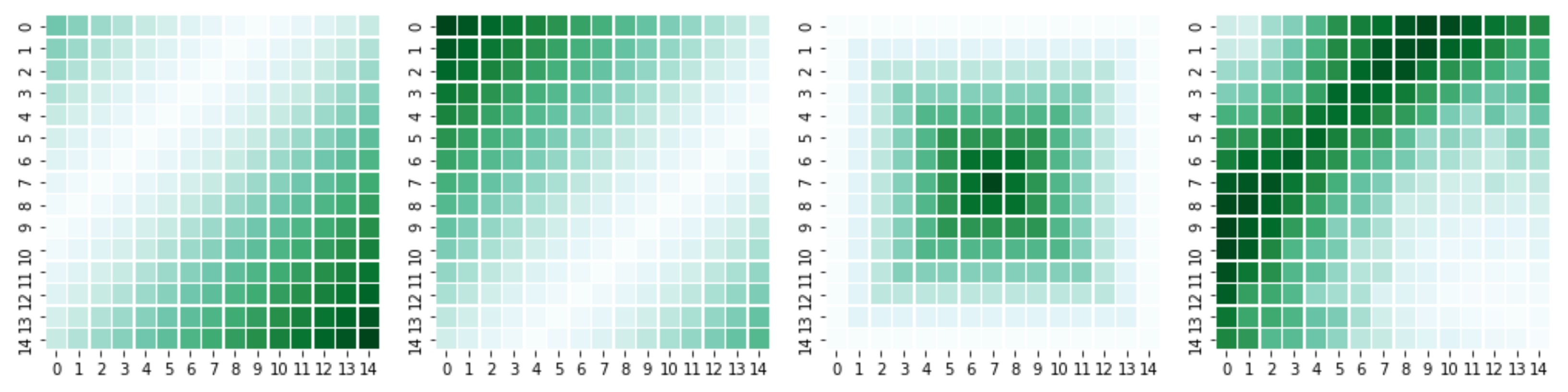
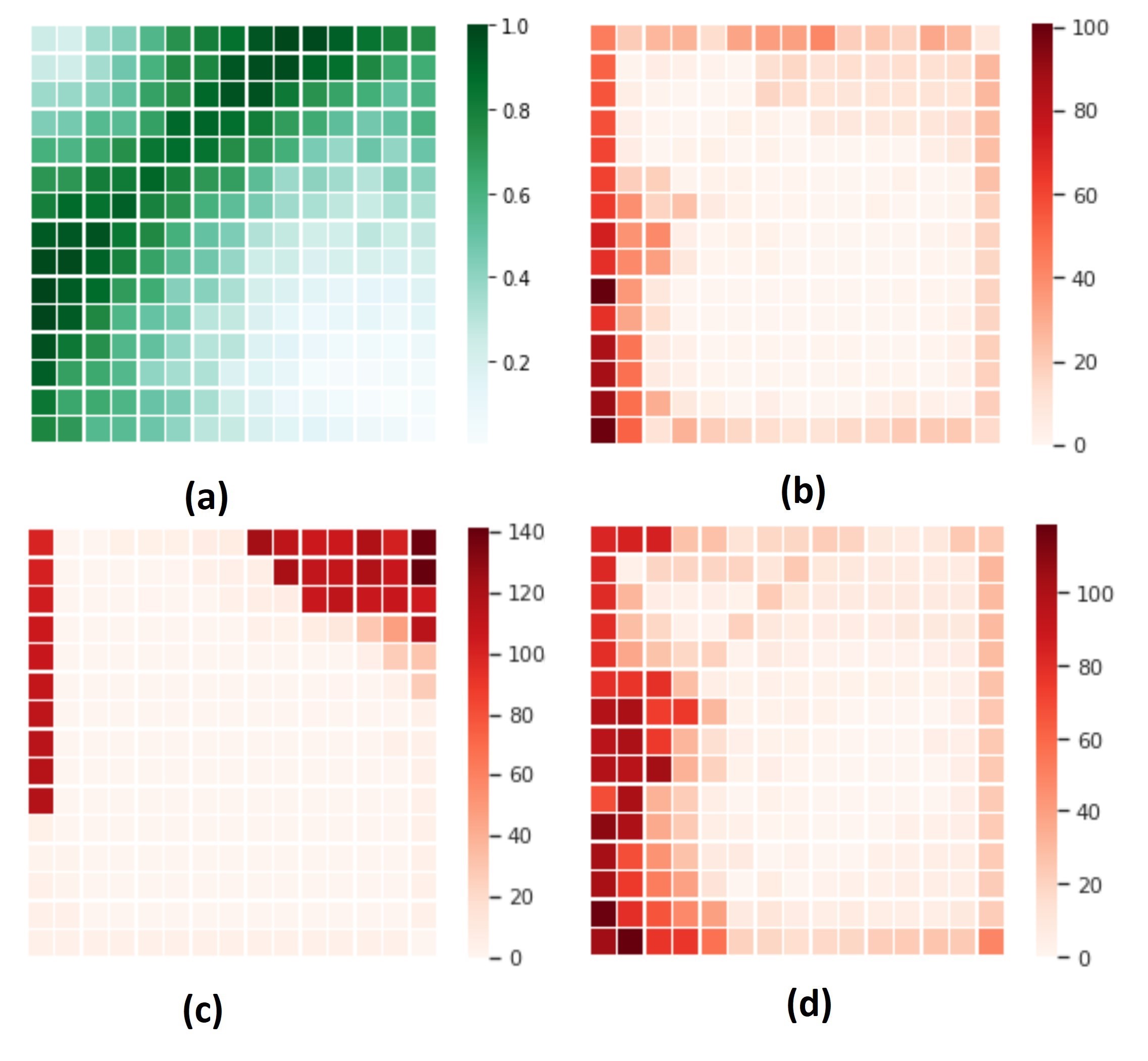
We perform experiments with two different kinds of animal densities : randomly distributed and spatially distributed. Here, we describe how we calculate spatially distributed animal densities. This distribution reflects the attractiveness of each cell in the park to a potential attacker. We assume that the distribution of targets that are of interest to attackers, is influenced by certain geographical and man-made features; namely : rivers, boundaries of the national park and roads (some of these features are used in (Gholami et al. 2018) to model attacker behavior).
We consider boundaries at all edges of the grid and we also consider that a river and a road pass through the national park. We then rank each cell depending on it’s distance from these features such that cells farther away have a higher rank, as shown in Fig. 4. We then take a weighted average of these ranks to get a measure of how attract a cell is to animals, with weights of 0.1, 0,1 and 0.8 given to the boundary, road and river ranks respectively and call it the animal rank. By further taking a weighted average of animal, river, road and boundary ranks with weights of 0.7, 0.05, 0.15 and 0.1, we arrive at the final animal density distribution.
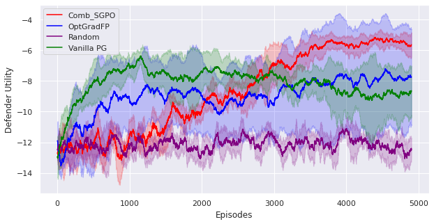
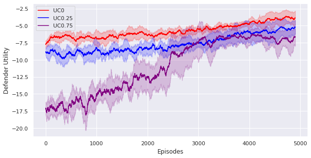
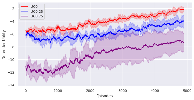
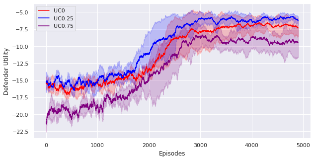
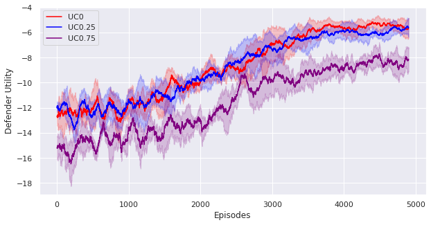
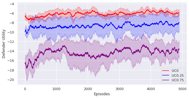
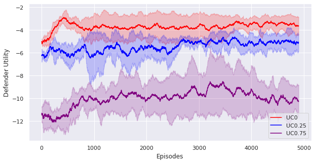
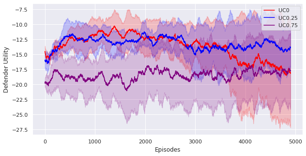
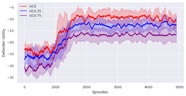
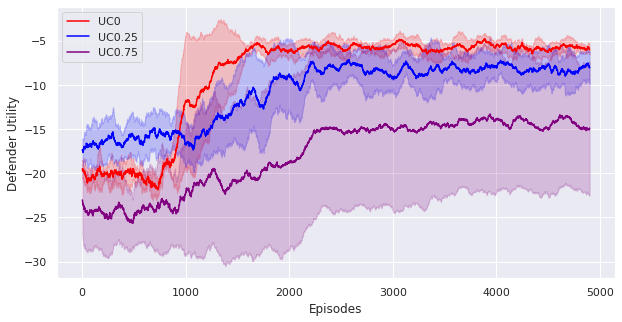
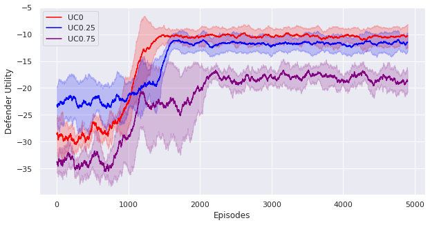
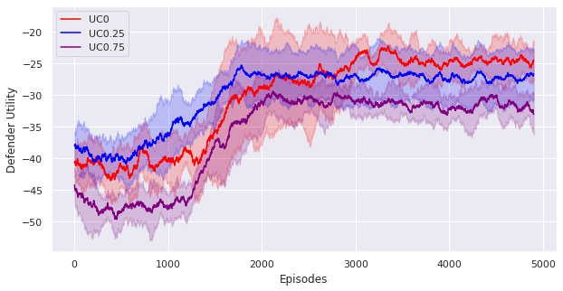
4 Additional Experiments
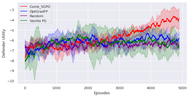
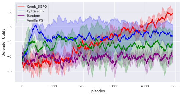
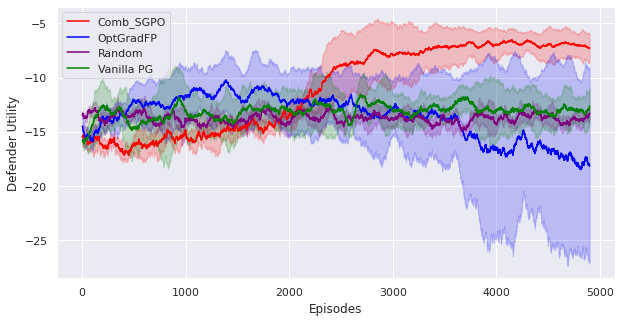
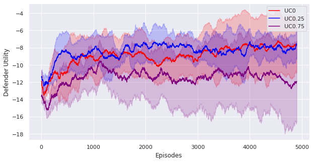
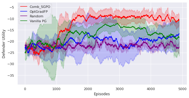
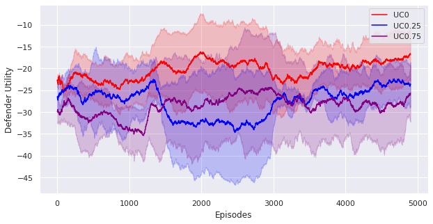
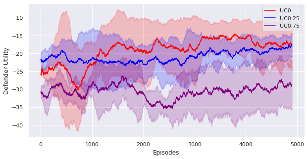
We show the learning curves for all baselines and CombSGPO under different uncertainty conditions in figures below, for gridsizes 15x15 and 10x10.
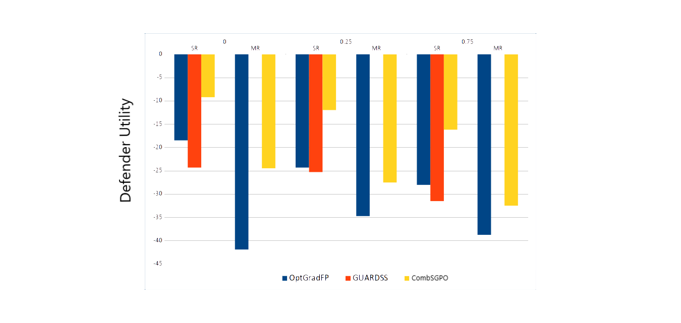


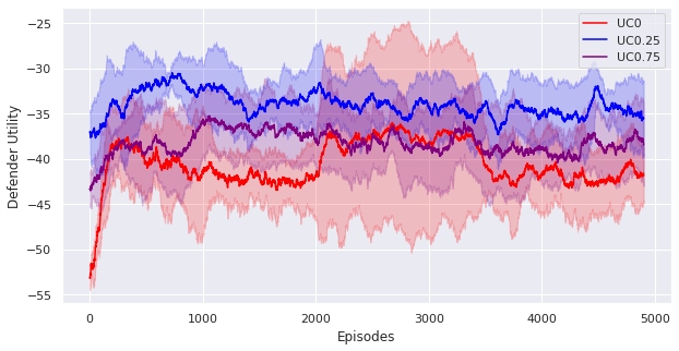
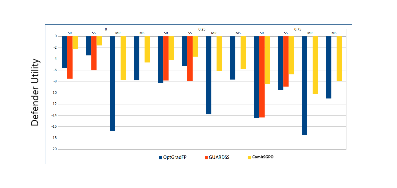
We also report the results for grid size which was used in GUARDSS paper. We observe from figure 7 that our model clearly outperforms OptGradFP and GUARDSS in all cases.