Hybrid Genetic Search for the CVRP: Open-Source Implementation and SWAP* Neighborhood

Abstract. The vehicle routing problem is one of the most studied combinatorial optimization topics, due to its practical importance and methodological interest. Yet, despite extensive methodological progress, many recent studies are hampered by the limited access to simple and efficient open-source solution methods. Given the sophistication of current algorithms, reimplementation is becoming a difficult and time-consuming exercise that requires extensive care for details to be truly successful. Against this background, we use the opportunity of this short paper to introduce a simple —open-source— implementation of the hybrid genetic search (HGS) specialized to the capacitated vehicle routing problem (CVRP). This state-of-the-art algorithm uses the same general methodology as Vidal et al. (2012) but also includes additional methodological improvements and lessons learned over the past decade of research. In particular, it includes an additional neighborhood called SWAP* which consists in exchanging two customers between different routes without an insertion in place. As highlighted in our study, an efficient exploration of SWAP* moves significantly contributes to the performance of local searches. Moreover, as observed in experimental comparisons with other recent approaches on the classical instances of Uchoa et al. (2017), HGS still stands as a leading metaheuristic regarding solution quality, convergence speed, and conceptual simplicity.

Keywords. Vehicle Routing Problem, Neighborhood Search, Hybrid Genetic Search, Open Source

1 Introduction

A decade has passed since the introduction of the hybrid genetic search with advanced diversity control (HGS in short) in Vidal et al. (2012) and the generalization of this method into a unified algorithm for the vehicle routing problem (VRP) family (Vidal et al. 2014, 2016, Vidal 2017, Vidal et al. 2021). Over this period, the method has produced outstanding results for an extensive collection of node and arc routing problems, and demonstrated that generality does not always hinder performance in this domain. As the VRP research community faces even more complex and integrated problems arising from e-commerce, home deliveries, and mobility-on-demand applications, efficient solution algorithms are more than ever instrumental for success (Vidal et al. 2020). Yet, new applications and management studies are often hampered by the need for efficient and scalable routing solution methods. The repeated invention and reproduction of heuristic solution methods turns into a time-consuming exercise that typically requires extensive care for details and systematic testing to be crowned with success. Moreover, the successful application of optimization algorithms rests on a delicate equilibrium. While the methods should be as sophisticated as required, they should also remain as simple and transparent as possible.

To facilitate future studies, we use the opportunity of this short paper to introduce an open-source HGS algorithm for the canonical capacitated vehicle routing problem (CVRP). We refer to this specialized implementation as HGS-CVRP. The C++ implementation of this algorithm has been designed to be transparent, specialized, and extremely concise, retaining only the core elements that make this method a success. Indeed, we believe that without any control on code complexity and length, it is almost always possible to achieve small performance gains through additional operators and method hybridizations, but at the cost of conceptual simplicity. We strive to avoid this pitfall as intricate designs tend to hinder scientific progress, and effectively deliver an algorithm based on two complementary operators: a crossover for diversification, and efficient local search strategies for solution improvement.

Beyond a simple reimplementation of the original algorithm, HGS-CVRP takes advantage of several lessons learned from the past decade of VRP studies: it relies on simple data structures to avoid move re-evaluations and uses the optimal linear-time Split algorithm of Vidal (2016). Moreover, its specialization to the CVRP permits significant methodological simplifications. In particular, it does not rely on the visit-pattern improvement (PI) operator (Vidal et al. 2012) originally designed for VRPs with multiple periods, and uses instead a new neighborhood called Swap*. As demonstrated in this paper, Swap* contains $\Theta(n^{4})$ moves but can be explored in sub-quadratic time. This neighborhood contains many improving moves that otherwise would not be identified. It can also be pruned by simple geometrical arguments, and largely contributes to the search performance. Our methodological developments are backed up by detailed experimental analyses which permit to evaluate the performance of HGS-CVRP and the contribution of Swap*. As observed in our results, this new algorithm reaches the same solution quality as the original HGS algorithm from Vidal et al. (2012) in a fraction of its computational time, and largely outperforms all other existing CVRP algorithms.

The remainder of this paper is structured as follows. Section 2 describes the HGS and its adaptations for the canonical CVRP. Section 3 presents the new Swap* neighborhood. Section 4 quickly discusses the structure of the open-source code. Section 5 details our computational experiments, and Section 6 finally concludes.

2 Hybrid Genetic Search for the CVRP

We consider a complete graph $G=(V,E)$ in which vertex $0$ represents a depot at which a fleet of $m$ vehicles is based, and the remaining vertices $\{1,\dots,n\}$ represent customer locations. Each edge $(i,j)\in E$ represents the possibility of traveling between locations $i$ and $j$ at a cost $c_{ij}$. The CVRP consists in determining up to $m$ vehicle routes starting and ending at the depot, in such a way that each customer is visited once, the total demand of the customers in any route does not exceed the vehicle capacity $Q$, and the sum of the distances traveled by the vehicles is minimized (Toth and Vigo 2014).

Our modern HGS-CVRP uses the same search scheme as the original method of Vidal et al. (2012). Its performance comes from a combination of three main strategies.

• A synergistic combination of crossover-based and neighborhood-based search, jointly evolving a population of individuals representing CVRP solutions. The former allows a diversified search in the solution space, while the latter permits aggressive solution improvement. Algorithms of this type are sometimes coined as memetic algorithms (Moscato and Cotta 2010).

• A controlled exploration of infeasible solutions, in which any excess load in the routes is linearly penalized. This allows focusing the search in regions that are close to the feasibility boundaries, where optimal or near-optimal solutions are more likely to belong (Glover and Hao 2011, Vidal et al. 2015).

• Advanced population diversity management strategies during parent and survivor selection, allowing to maintain a diversified and high-quality set of solutions and counterbalance the loss of diversity due to the neighborhood search.
  

The general structure of the search is represented in Figure 1. After a population initialization phase, the algorithm iteratively generates new solutions by 1) selecting two parents, 2) recombining them to produce a new solution, 3) improving this solution with a local search, and 4) inserting the result in the population. This process is repeated until a termination criterion is attained, typically a number of consecutive iterations $N_{\textsc{it}}$ without improvement or a time limit $T_{\textsc{max}}$.

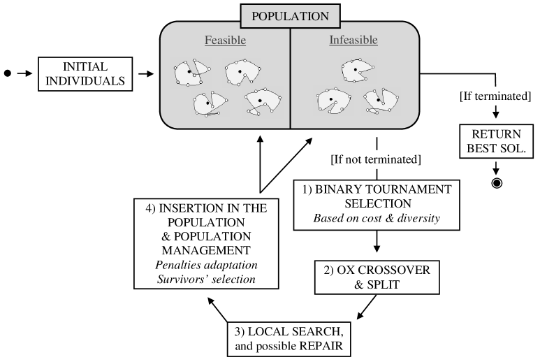
Figure 1: General structure of the hybrid genetic search

Parents Selection. To select each parent, the algorithm performs a binary tournament selection consisting in randomly picking, with uniform probability, two individuals and retaining the one with the best fitness. It is noteworthy that the notion of fitness in HGS is based on objective value and diversity considerations. Each individual $S$ is therefore characterized by (i) its rank $f_{\mathcal{P}}^{\phi}(S)$ in terms of solution quality, and (ii) its rank in terms of diversity contribution $f_{\mathcal{P}}^{\textsc{div}}(S)$, measured as its average broken-pairs distance to its $n_{\textsc{Closest}}$ most similar solutions in the population ${\mathcal{P}}$. Its fitness is then calculated as a weighted sum of these ranks as:

$$f_{\mathcal{P}}(S)=f_{\mathcal{P}}^{\phi}(S)+\left(1-\frac{n^{\textsc{Elite}}}{|{\mathcal{P}}|}\right)f_{\mathcal{P}}^{\textsc{div}}(S).$$ (1)

This equation sets a slightly larger weight on solution quality to ensure that the top $n_{\textsc{Elite}}$ best individuals are preserved during the search.

Recombination. HGS applies an ordered crossover (OX – Oliver et al. 1987) on a simple permutation-based representation of the two parents. As seen on Figure 2, OX consists in inheriting a random fragment of the first parent, and then completing missing visits using the sequence of the second parent. This representation omits the visits to the depot, in such a way that capacity constraints are disregarded in the crossover. This design choice is convenient since there exists a dynamic programming algorithm, called Split, capable of optimally re-inserting trip delimiters in the crossover’s output to produce a complete CVRP solution (Beasley 1983, Prins 2004). In HGS-CVRP, we rely on the efficient linear-time Split algorithm introduced by Vidal (2016) after each crossover operation.

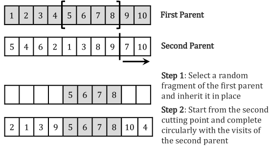
Figure 2: OX Crossover

Neighborhood Search. An efficient local search is applied to each solution resulting from the crossover and Split algorithms. In the original algorithm of Vidal et al. (2012), this search included two stages: route improvement (RI) and pattern improvement (PI). The RI local search uses Swap and Relocate moves, generalized to sequences of two consecutive nodes, as well as 2-Opt and 2-Opt*. The neighborhoods are limited to moves involving geographically close node pairs $(i,j)$ such that $j$ belongs to the $\Gamma$ closest clients from $i$. The granularity parameter $\Gamma$ therefore limits the neighborhoods’ size to ${\mathcal{O}}(\Gamma n)$. The exploration of the moves is organized in random order of the indices $i$ and $j$ and any improving move is immediately applied. This process is pursued until attaining a local minimum. The pattern improvement (PI) phase of Vidal et al. (2012) was originally designed to optimize the assignment of client visits to days or depots, for VRP variants with multiple periods or depots. We excluded this mechanism in HGS-CVRP, and instead included an additional neighborhood in RI called Swap*, described in Section 3.

Due to the controlled exploration of infeasible solutions, is it possible for a solution to remain infeasible after the local search. When this happens, a Repair operation is applied with $50\%$ probability. This operation consists of running the local search with ($10\times$) higher penalty coefficients, aiming to recover a feasible solution.

Population management. HGS maintains two subpopulations: for feasible and infeasible solutions, respectively. Each individual produced in the previous steps is directly included in the adequate subpopulation. Each subpopulation is managed to contain between $\mu$ and $\mu+\lambda$ solutions in such a way that the parameter $\mu$ represents a minimum population size and parameter $\lambda$ is a generation size. Initially, $4\mu$ random solutions are generated, improved through local search, and included in the subpopulations according to their feasibility. Whenever a subpopulation reaches $\mu+\lambda$ individuals, a survivors selection phase is triggered to iteratively eliminate $\lambda$ solutions. This is done by iteratively removing a clone solution (i.e., identical to another one) if such a solution exists, or otherwise the worst solution in terms of fitness according to Equation (1).

The penalty parameters for solution infeasibility are adapted through the search to achieve a target ratio $\xi^{\textsc{ref}}$ of feasible solutions at the end of the local search (LS). This is done by monitoring the number of feasible solutions obtained at regular intervals and increasing or decreasing the penalty coefficient by a small factor to achieve the desired target ratio, as in Vidal et al. (2012). Finally, to deliver a method that remains as conceptually simple as possible, we did not include additional diversification phases in HGS-CVRP. The complete method is summarized in Algorithm 1.

1 Initialize population with random solutions improved by local search;

2 while number of iterations without improvement $<It_{\textsc{ni}}$ and time $<T_{\textsc{max}}$ do

3       Select parent solutions $P_{1}$ and $P_{2}$;

4       Apply the crossover operator on $P_{1}$ and $P_{2}$ to generate an offspring $C$;

5       Educate offspring $C$ by local search;

6       Insert $C$ into respective subpopulation;

7       if $C$ is infeasible then

8             With 50% probability, repair $C$ (local search) and insert it into respective subpopulation;

9            

10      if maximum subpopulation size reached then

11             Select survivors;

12            

13      Adjust penalty coefficients for infeasibility;

14      

15Return best feasible solution;

Algorithm 1 HGS-CVRP

3 The SWAP* Neighborhood

The classical Swap neighborhood exchanges two customers in place (i.e., one replaces the other and vice-versa). This neighborhood is typically used for intra-route and inter-route improvements. In contrast, the proposed Swap* neighborhood consists in exchanging two customers $v$ and $v^{\prime}$ from different routes $r$ and $r^{\prime}$ without an insertion in place. In this process, $v$ can be inserted in any position of $r^{\prime}$, and $v^{\prime}$ can likewise be inserted in any position of $r$. Evaluating all the Swap* moves would take a computational time proportional to $\Theta(n^{3})$ with a direct implementation. However, more efficient search strategies exist. In particular, Theorem 1 permits us to cut down this complexity.

Theorem 1

In a best Swap* move between customers $v$ and $v^{\prime}$ within routes $r$ and $r^{\prime}$, the new insertion position of $v$ in $r^{\prime}$ is either:

1. in place of $v^{\prime}$, or

2. among the three best insertion positions in $r^{\prime}$ as evaluated prior to the removal of $v^{\prime}$.

A symmetrical argument holds for the new insertion position of $v^{\prime}$ in $r$.

Proof. Let $P(r)=\{(0,r_{1}),(r_{1},r_{2}),\dots,(r_{|r|-1},r_{|r|}),(r_{|r|},0)\}$ be the set of edges representing possible insertion positions in a route $r=(r_{1},\dots,r_{|r|})$. The insertion cost of a vertex $v$ in a position $(i,j)\in P(r)$ is evaluated as $\Delta(v,i,j)=c_{iv}+c_{vj}-c_{ij}$. The best insertion cost of a vertex $v$ in a route $r$ is calculated as $\Delta^{\textsc{min}}(v,r)=\min_{(i,j)\in P(r)}\Delta(v,i,j)$.

Let $v^{\prime}_{\textsc{p}}$ and $v^{\prime}_{\textsc{s}}$ represent the predecessor and successor of $v^{\prime}$ in its original route $r^{\prime}$. After removal of $v^{\prime}$, the best insertion cost of vertex $v$ in the resulting route $\hat{r}^{\prime}$ is calculated as:

$$\Delta^{\textsc{min}}(v,\hat{r}^{\prime})=\min\{\Delta(v,v^{\prime}_{\textsc{p}},v^{\prime}_{\textsc{s}}),\min_{(i,j)\in\mathcal{P}}\Delta(v,i,j)\},$$ (2)

$$\text{where }\mathcal{P}=P(r^{\prime})-\{(v^{\prime}_{\textsc{p}},v^{\prime}),(v^{\prime},v^{\prime}_{\textsc{s}})\}.$$ (3)

The first term of Equation (2) represents an insertion in place of $v^{\prime}$ (first statement of Theorem 1), whereas the second term corresponds to a minimum value over $P(r^{\prime})$ without two elements. Therefore, this minimum is necessarily attained for one of the three best values over $P(r^{\prime})$.$\hfill\Box$

Algorithm 2 builds on Theorem 1 to provide an efficient search strategy for Swap*. The neighborhood exploration is organized by route pairs $r$ and $r^{\prime}$ (Lines 1–2), firstly preprocessing the three best insertion positions of each customer $v\in r$ into $r^{\prime}$ (Lines 3–4) and of each customer $v\in r^{\prime}$ into $r$ (Lines 5–6), and then exploiting this information to find the best move for each node $v\in r$ and $v^{\prime}\in r^{\prime}$ (Lines 8–16). Since the preprocessed information is valid until the routes have been modified, we use a move acceptance strategy that consists in applying the best Swap* move per route pair (Lines 17–18).

1 for each route $r\in\mathcal{R}$ do

2       for each route $r^{\prime}$ in $\Gamma^{\textsc{R}}(r)$ do

3             for each customer vertex $v\in r$ do $\triangleright$ Preprocessing Phase

4                   $((i_{1v},j_{1v}),(i_{2v},j_{2v}),(i_{3v},j_{3v}))\leftarrow\textsc{FindTop3Locations}(v,r^{\prime})$

5            for each customer vertex $v^{\prime}\in r^{\prime}$ do

6                   $((i_{1v^{\prime}},j_{1v^{\prime}}),(i_{2v^{\prime}},j_{2v^{\prime}}),(i_{3v^{\prime}},j_{3v^{\prime}}))\leftarrow\textsc{FindTop3Locations}(v^{\prime},r)$

7            $\Delta_{\textsc{best}}=0$

8             for each customer vertex $v\in r$ do $\triangleright$ Search Phase

9                   for each customer vertex $v^{\prime}\in r^{\prime}$ do

10                         $k\,=\min\{\kappa\,|\,i_{\kappa v}\neq v^{\prime}\text{ and }j_{\kappa v}\neq v^{\prime}\}$

11                         $k^{\prime}=\min\{\kappa\,|\,i_{\kappa v^{\prime}}\neq v\text{ and }j_{\kappa v^{\prime}}\neq v\}$

12                         $\Delta_{v\rightarrow r^{\prime}}=\min\{\Delta(v,v^{\prime}_{\textsc{p}},v^{\prime}_{\textsc{s}}),\Delta(v,i_{kv},j_{kv})\}-\Delta(v,v_{\textsc{p}},v_{\textsc{s}})$

13                         $\Delta_{v^{\prime}\rightarrow r}=\min\{\Delta(v^{\prime},v_{\textsc{p}},v_{\textsc{s}}),\Delta(v^{\prime},i_{k^{\prime}v^{\prime}},j_{k^{\prime}v^{\prime}})\}-\Delta(v^{\prime},v^{\prime}_{\textsc{p}},v^{\prime}_{\textsc{s}})$

14                         if $\Delta_{v\rightarrow r^{\prime}}+\Delta_{v^{\prime}\rightarrow r}<\Delta_{\textsc{best}}$ then

15                               $\Delta_{\textsc{best}}=\Delta_{v\rightarrow r^{\prime}}+\Delta_{v^{\prime}\rightarrow r}$

16                               $(v_{\textsc{best}},v^{\prime}_{\textsc{best}})=(v,v^{\prime})$

17            if $\Delta_{\textsc{best}}<0$ then

18                   $\textsc{ApplySwap*}(v_{\textsc{best}},v^{\prime}_{\textsc{best}})$

Algorithm 2 Efficient exploration of the Swap* neighborhood

Each call to the function $\textsc{FindTop3Locations}(v,r)$ requires a computational time proportional to the size of the route $r$. Therefore, the computational time of Algorithm 2 grows as

$$\Phi=\sum_{r\in\mathcal{R}}\sum_{r^{\prime}\in\mathcal{R}}\left(\sum_{v\in r}|r^{\prime}|+\sum_{\smash{v^{\prime}\in r^{\prime}}}|r|+\sum_{v\in r}\sum_{\smash{v^{\prime}\in r^{\prime}}}1\right)={\mathcal{O}}\left(\sum_{r\in\mathcal{R}}\sum_{r^{\prime}\in\mathcal{R}}|r||r^{\prime}|\right)={\mathcal{O}}(n^{2}).$$ (4)

Since a quadratic-time algorithm may still represent a bottleneck for large instances, we opted to restrict further the route pairs $(r,r^{\prime})$ considered at Lines 3 and 4 using simple geometric arguments. We therefore only evaluate Swap* moves between $r$ and $r^{\prime}$ if the polar sectors (from the depot) associated with these routes intercept each other. As shown in our computational experiments, with this additional restriction, the computational effort needed to explore Swap* decreases and becomes comparable to that of other standard neighborhoods in RI. Note that the computation of polar sectors for each route requires location information for client requests (e.g., latitude/longitude or a proxy thereof). Other relatedness measures between routes (e.g., distance information or search history) could be alternatively used if such information is unavailable.

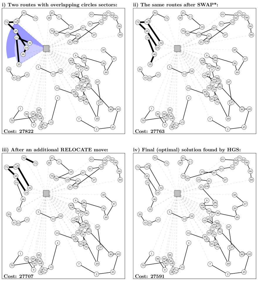
Figure 3: Illustration of the Swap* neighborhood on instance X-n101-k25

Figure 3 illustrates the Swap* neighborhood during one execution of HGS-CVRP on instance X-n101-k25 from Uchoa et al. (2017). Four solutions are represented. The trips from and to the depot are presented with dashes to enhance readability. Solution (i) is a local minimum of all standard CVRP neighborhoods (Swap, Relocate, 2-opt and 2-opt*). Still, Swap* can identify a critical improvement between two routes highlighted in boldface on the figure. Applying this move permits to reduce the number of route intersections without violating capacity constraints. Moreover, it permits a follow-up improvement with Relocate, leading to Solution (iii). It is noteworthy that the solution resulting from these moves exhibits the same route arrangement in the top left quadrant as Solution (iv), which is known to be optimal for this instance.

4 Open-Source Implementation

Our open-source implementation is provided at https://github.com/vidalt/HGS-CVRP. The code includes six main classes.

• [Individual] represents the solutions (i.e., individuals of the genetic algorithm) through the search. For convenience, we store complete solutions including trip delimiters along with their associated giant tours. According to this design, the trip delimiters are immediately recalculated after crossover using the Split algorithm. This facilitates solution manipulation, feasibility checks, and distance calculations (when evaluating population diversity).

• [Population] holds the two subpopulations. It also contains efficient data structures to memorize the distances between solutions used in the diversity calculations.

• [Genetic] contains the main structure of the genetic algorithm and the crossover operator.

• [Split] contains the linear split algorithm as introduced in Vidal (2016).

• [LocalSearch] provides all the functions needed for the local search, including the Swap* exploration procedure which is directly embedded after the other neighborhoods. Without doubt, this is the most time-critical component of the algorithm. To efficiently represent and update the incumbent solution, we use a specialized array data structure for indexed access in $O(1)$, along with pointers giving access to the predecessors and successors in the routes. This allows efficient preprocessing, move evaluations, and solution modifications. We also use a smart data structure to register the moves that have already been tested without improvement. Instead of using binary “move descriptors” (see, e.g., Zachariadis and Kiranoudis 2010) which require a substantial computational effort for reinitialization upon modification of a route, we rely on integer “time stamps” to register “when” a route was last modified, and “when” the moves associated to a given customer were last evaluated. Any non-decreasing counter can be used as a representation of time. We opted to use the number of applied moves for that purpose. A simple $O(1)$ comparison of the time stamps permits to quickly determine if the routes have been modified since the last move evaluation, and no reinitialization is needed when a route is modified.

• [CircleSector] contains elementary routines to calculate polar sectors and their intersections for Swap*.

• [Params], [Commandline] and [main] finally store the parameters of the algorithm and permit to launch the code. The method is driven by only six parameters summarized in Table 1. All of these parameters have been set to the original values calibrated in Vidal et al. (2012), except $n_{\textsc{Elite}}$ which has been lowered down to $n_{\textsc{Elite}}=4$ to favor diversity and counterbalance the additional convergence due to the Swap* neighborhood.

  Table 1: Parameters of HGS-CVRP

  Parameter		Value
  $\mu$	Population size	25
  $\lambda$	Generation size	40
  $n_{\textsc{Elite}}$	Number of elite solutions considered in the fitness calculation	4
  $n_{\textsc{Closest}}$	Number of close solutions considered in the diversity-contribution measure	5
  $\Gamma$	Granular search parameter	20
  $\xi^{\textsc{ref}}$	Target proportion of feasible individuals for penalty adaptation	0.2

  The algorithm can be run with a termination criterion based on a number of consecutive iterations without improvement N${}_{\textsc{it}}$ (20,000 per default) or a CPU time limit T${}_{\textsc{max}}$. In the latter case, the algorithm restarts after each N${}_{\textsc{it}}$ iterations without improvement and collects the best solution until the time limit.

5 Experimental Analyses

Good testing practices in optimization call for code comparisons on similar computing environments with the same number of threads (usually one) and time (Talbi 2009, Kendall et al. 2016). CPU time and solution quality cannot be examined separately, such that claims about fast solutions without a critical evaluation of solution quality are mainly inconclusive. Indeed, CPU time is often a direct consequence of the choice of termination criterion and parameters (when it is not itself the termination criterion) and is best seen as a factor rather than an experimental outcome.

There exist different ways to consider speed and solution quality jointly in experimental analyses. A first generic approach is to opt for a bi-objective evaluation (e.g., in Figure 4.3 of Laporte et al. 2014) to identify non-dominated methods. Another intuitive approach, typical in bi-objective analyses, is to fix one dimension and measure the other, by either setting the same CPU-time limit for all algorithms or a target solution quality to achieve (Aiex et al. 2007, Talbi 2009). Lastly, one could compare the complete convergence profiles of different algorithms during their execution by measuring solution quality over time. This approach provides the most insights, but it requires additional intervention into the algorithms to collect the solution values found throughout the search. We will favor this approach since we have access to the implementation of the algorithms being compared.

Our computational experiments follow two primary goals. Firstly, we evaluate the impact of our main methodological proposal —the Swap* neighborhood— by comparing two method variants: the original HGS (referred to as HGS-2012 in the following) with its modern HGS-CVRP implementation using Swap*. Second, we extend our experimental comparison to other CVRP heuristics to compare their convergence behavior using the same computational environment. For this analysis, we consider recent algorithms representative of the current academic state-of-the-art:

• the hybrid iterated local search (HILS) of Subramanian et al. (2013);

• the Lin-Kernighan-Helsgaun (LKH-3) heuristic of Helsgaun (2017);

• the knowledge guided local search (KGLS) of Arnold and Sörensen (2018);

• the slack induction by string removals (SISR) of Christiaens and Vanden Berghe (2020);

• the fast iterative localized optimization (FILO) algorithm of Accorsi and Vigo (2021).

We were given access to the authors’ implementations of HILS, LKH-3, and FILO, as well as to an executable library for KGLS. The original implementation of SISR was unavailable, but we had access to a faithful reproduction of this algorithm from Guillen et al. (2020), which achieves solutions of a quality which is statistically indistinguishable from that of the original algorithm in a similar or slightly shorter amount of time. Finally, we also establish a comparison with the solver provided by Google OR-Tools at https://github.com/google/or-tools, since this algorithm is often used in practical applications. We use the guided local search (GLS) variant of this solver as recommended in the documentation. To our knowledge, this is one of the first analyses to evaluate such a wide diversity of state-of-the-art algorithm implementations on a single test platform.

We conduct our experiments on the 100 classical benchmark instances of Uchoa et al. (2017), as they cover diverse characteristics (e.g., distribution of demands, customer and depot positioning, route length) and represent a significant challenge for modern algorithms. HGS-2012, HGS-CVRP, HILS, LKH-3, FILO, and OR-Tools have been developed in C/C++ and compiled with g++ 9.1.0, while KGLS and SISR use Java OpenJDK 13.0.1. All experiments are run on a single thread of an Intel Gold 6148 Skylake 2.4 GHz processor with 40 GB of RAM, running CentOS 7.8.2003.

We monitor each algorithm’s progress up to a time limit of $T_{\textsc{max}}=n\times 240/100$ seconds, where $n$ represents the number of customers. Therefore, the smallest instance with $100$ clients is run for $4$ minutes, whereas the largest instance containing $1000$ clients is run for $40$ minutes. During each run, we record the best solution value after 1%, 2%, 5%, 10%, 15%, 20%, 30%, 50%, 75%, and 100% of the time limit to measure the performance of the algorithms at different stages of the search. To increase statistical significance, we perform ten independent runs with different seeds. For KGLS and OR-tools, we use different random permutations of the customers in the data file, since these two algorithms are deterministic but depend on the order of the customers in the data (in this case, the permutation of the customers effectively acts as a seed). We finally calculate the percentage gap of each algorithm as $\text{Gap}=100\times(z-z_{\textsc{BKS}})/z_{\textsc{BKS}}$, where $z$ is the solution value of the algorithm and $z_{\textsc{BKS}}$ is the best known solution (BKS) value for this instance, as listed on the CVRPLIB website at http://vrp.atd-lab.inf.puc-rio.br/index.php/en/.

Table 2: Comparison of average solution quality over ten runs and gap at $T_{\textsc{max}}$

Instance		OR-Tools			LKH-3			HILS			KGLS			SISR			FILO			HGS-2012			HGS-CVRP			BKS
		Avg	Gap		Avg	Gap		Avg	Gap		Avg	Gap		Avg	Gap		Avg	Gap		Avg	Gap		Avg	Gap
X-n101-k25		27977.2	1.40		27639.2	0.17		27591.0	0.00		27631.9	0.15		27593.3	0.01		27591.0	0.00		27591.0	0.00		27591.0	0.00		27591
X-n106-k14		26757.5	1.50		26406.8	0.17		26391.1	0.11		26413.2	0.19		26380.9	0.07		26373.3	0.04		26408.8	0.18		26381.4	0.07		26362
X-n110-k13		15099.8	0.86		14993.9	0.15		14971.0	0.00		14971.0	0.00		14972.1	0.01		14971.0	0.00		14971.0	0.00		14971.0	0.00		14971
X-n115-k10		12808.3	0.48		12747.0	0.00		12747.0	0.00		12747.1	0.00		12747.0	0.00		12747.0	0.00		12747.0	0.00		12747.0	0.00		12747
X-n120-k6		13501.9	1.27		13332.8	0.01		13333.7	0.01		13332.0	0.00		13332.0	0.00		13332.0	0.00		13332.0	0.00		13332.0	0.00		13332
X-n125-k30		56853.4	2.37		55907.4	0.66		55846.5	0.55		55740.8	0.36		55559.8	0.04		55693.7	0.28		55539.0	0.00		55539.0	0.00		55539
X-n129-k18		29722.3	2.70		29083.3	0.50		28972.1	0.11		28971.6	0.11		28948.9	0.03		28948.4	0.03		28940.0	0.00		28940.0	0.00		28940
X-n134-k13		11171.0	2.34		10970.6	0.50		10947.5	0.29		10940.5	0.22		10937.7	0.20		10927.9	0.11		10916.0	0.00		10916.0	0.00		10916
X-n139-k10		13741.2	1.11		13654.9	0.48		13591.2	0.01		13590.0	0.00		13590.4	0.00		13590.0	0.00		13590.0	0.00		13590.0	0.00		13590
X-n143-k7		16135.6	2.77		15767.8	0.43		15735.7	0.23		15730.6	0.19		15727.8	0.18		15723.8	0.15		15700.0	0.00		15700.0	0.00		15700
X-n148-k46		44598.5	2.65		43518.9	0.16		43448.0	0.00		43588.3	0.32		43464.1	0.04		43480.5	0.07		43448.0	0.00		43448.0	0.00		43448
X-n153-k22		21789.3	2.68		21240.8	0.10		21452.3	1.09		21386.0	0.78		21228.6	0.04		21232.9	0.06		21223.5	0.02		21225.0	0.02		21220
X-n157-k13		17137.7	1.55		16879.1	0.02		16876.0	0.00		16877.5	0.01		16878.2	0.01		16876.0	0.00		16876.0	0.00		16876.0	0.00		16876
X-n162-k11		14262.2	0.88		14173.7	0.25		14152.4	0.10		14147.0	0.06		14159.0	0.15		14157.5	0.14		14138.0	0.00		14138.0	0.00		14138
X-n167-k10		21176.4	3.01		20706.1	0.73		20603.7	0.23		20586.9	0.15		20558.6	0.01		20557.0	0.00		20557.0	0.00		20557.0	0.00		20557
X-n172-k51		46874.9	2.78		45788.1	0.40		45665.3	0.13		45802.8	0.43		45622.6	0.03		45607.0	0.00		45607.0	0.00		45607.0	0.00		45607
X-n176-k26		49260.2	3.03		48104.1	0.61		48218.5	0.85		47991.6	0.38		47823.7	0.02		47985.0	0.36		47812.0	0.00		47812.0	0.00		47812
X-n181-k23		25935.6	1.43		25627.0	0.23		25572.1	0.01		25602.3	0.13		25575.1	0.02		25569.2	0.00		25570.2	0.00		25569.0	0.00		25569
X-n186-k15		24908.0	3.16		24277.7	0.55		24170.7	0.11		24178.3	0.14		24166.2	0.09		24154.6	0.04		24145.2	0.00		24145.0	0.00		24145
X-n190-k8		17421.9	2.60		17074.7	0.56		17108.0	0.75		17033.5	0.32		16982.8	0.02		16984.3	0.03		16992.4	0.07		16983.3	0.02		16980
X-n195-k51		46151.1	4.36		44478.8	0.57		44305.0	0.18		44427.2	0.46		44292.0	0.15		44265.7	0.09		44225.0	0.00		44225.0	0.00		44225
X-n200-k36		60447.9	3.19		58913.6	0.57		58784.0	0.35		58828.0	0.43		58635.6	0.10		58806.9	0.39		58589.6	0.02		58578.0	0.00		58578
X-n204-k19		20348.4	4.00		19731.3	0.85		19617.6	0.27		19621.0	0.29		19653.2	0.45		19568.4	0.02		19565.0	0.00		19565.0	0.00		19565
X-n209-k16		31775.5	3.65		30925.0	0.88		30739.0	0.27		30709.7	0.18		30661.7	0.02		30684.4	0.09		30658.7	0.01		30656.0	0.00		30656
X-n214-k11		11374.0	4.77		11103.4	2.28		11077.2	2.04		10944.3	0.81		10894.4	0.35		10884.3	0.26		10877.0	0.19		10860.5	0.04		10856
X-n219-k73		118038.0	0.38		117669.3	0.06		117595.0	0.00		117689.1	0.08		117623.7	0.02		117595.1	0.00		117601.7	0.01		117596.1	0.00		117595
X-n223-k34		42046.6	3.98		40750.9	0.78		40549.8	0.28		40714.4	0.69		40535.5	0.24		40502.8	0.16		40455.3	0.05		40437.0	0.00		40437
X-n228-k23		26613.4	3.39		25879.8	0.54		25803.7	0.24		25836.8	0.37		25814.3	0.28		25781.7	0.15		25742.7	0.00		25742.8	0.00		25742
X-n233-k16		19883.9	3.40		19345.8	0.60		19296.0	0.34		19328.6	0.51		19285.7	0.29		19293.9	0.33		19233.1	0.02		19230.0	0.00		19230
X-n237-k14		27927.5	3.27		27164.0	0.45		27068.8	0.10		27095.9	0.20		27081.1	0.14		27050.8	0.03		27049.4	0.03		27042.0	0.00		27042
X-n242-k48		85518.0	3.34		83353.0	0.73		82867.9	0.14		83209.2	0.55		82885.6	0.16		82876.1	0.15		82826.5	0.09		82806.0	0.07		82751
X-n247-k50		38282.8	2.71		37412.2	0.37		37502.3	0.61		37388.4	0.31		37379.6	0.28		37453.6	0.48		37295.0	0.06		37277.1	0.01		37274
X-n251-k28		40087.6	3.63		38982.0	0.77		38859.4	0.45		38893.3	0.54		38765.2	0.21		38783.5	0.26		38735.9	0.13		38689.9	0.02		38684
X-n256-k16		19294.5	2.42		19086.6	1.31		18880.8	0.22		18891.6	0.28		18887.3	0.26		18880.0	0.22		18880.0	0.22		18839.6	0.00		18839
X-n261-k13		27920.6	5.13		27115.6	2.10		26808.2	0.94		26717.5	0.60		26595.8	0.14		26682.4	0.47		26594.0	0.14		26558.2	0.00		26558

Table 3: Comparison of average solution quality over ten runs and gap at $T_{\textsc{max}}$ (continued)

Instance		OR-Tools			LKH-3			HILS			KGLS			SISR			FILO			HGS-2012			HGS-CVRP			BKS
		Avg	Gap		Avg	Gap		Avg	Gap		Avg	Gap		Avg	Gap		Avg	Gap		Avg	Gap		Avg	Gap
X-n266-k58		77660.8	2.89		76117.7	0.85		75611.4	0.18		75954.6	0.63		75609.2	0.17		75767.0	0.38		75646.8	0.22		75564.7	0.11		75478
X-n270-k35		36700.5	3.99		35523.3	0.66		35352.9	0.18		35462.1	0.48		35364.4	0.21		35348.3	0.16		35306.4	0.04		35303.0	0.03		35291
X-n275-k28		22087.3	3.96		21340.5	0.45		21262.4	0.08		21299.4	0.26		21250.5	0.03		21251.1	0.03		21247.8	0.01		21245.0	0.00		21245
X-n280-k17		35055.6	4.63		33933.6	1.29		33803.4	0.90		33670.1	0.50		33648.6	0.43		33652.6	0.45		33573.0	0.21		33543.2	0.12		33503
X-n284-k15		21137.9	4.57		20521.2	1.51		20415.9	0.99		20360.0	0.72		20287.6	0.36		20273.5	0.29		20248.0	0.16		20245.5	0.15		20215
X-n289-k60		98560.9	3.58		96055.6	0.95		95515.0	0.38		95882.8	0.77		95345.8	0.20		95556.3	0.43		95350.4	0.21		95300.9	0.16		95151
X-n294-k50		49301.8	4.54		47538.6	0.80		47262.0	0.21		47454.1	0.62		47251.9	0.19		47273.3	0.24		47217.8	0.12		47184.1	0.05		47161
X-n298-k31		36970.5	8.00		34571.7	1.00		34383.7	0.45		34377.4	0.43		34267.8	0.11		34283.3	0.15		34235.9	0.01		34234.8	0.01		34231
X-n303-k21		22573.7	3.85		22008.0	1.25		21900.7	0.76		21903.4	0.77		21772.9	0.17		21809.1	0.34		21763.4	0.13		21748.5	0.06		21736
X-n308-k13		27141.4	4.96		26194.9	1.30		26058.6	0.77		26076.4	0.84		26281.0	1.63		25937.7	0.30		25879.8	0.08		25870.8	0.05		25859
X-n313-k71		97497.4	3.67		94974.7	0.99		94290.3	0.26		94763.8	0.77		94155.7	0.12		94351.6	0.33		94127.7	0.09		94112.2	0.07		94043
X-n317-k53		79211.0	1.09		78553.5	0.25		78355.0	0.00		78413.5	0.07		78386.1	0.04		78358.6	0.00		78374.8	0.03		78355.4	0.00		78355
X-n322-k28		31488.5	5.55		30253.4	1.41		29996.5	0.54		30038.0	0.68		29892.5	0.20		29934.9	0.34		29887.5	0.18		29848.7	0.05		29834
X-n327-k20		28777.6	4.52		27905.1	1.36		27815.8	1.03		27646.8	0.42		27644.7	0.41		27610.7	0.29		27580.4	0.18		27540.8	0.03		27532
X-n331-k15		32648.2	4.97		31336.1	0.75		31227.4	0.40		31200.1	0.32		31124.5	0.07		31103.1	0.00		31114.0	0.04		31103.0	0.00		31102
X-n336-k84		143294.8	3.01		140226.2	0.80		139560.0	0.32		140831.3	1.24		139429.8	0.23		139585.7	0.34		139437.1	0.23		139273.5	0.12		139111
X-n344-k43		44036.4	4.72		42625.4	1.37		42307.5	0.61		42350.5	0.71		42122.7	0.17		42174.2	0.30		42086.0	0.09		42075.6	0.06		42050
X-n351-k40		27433.6	5.94		26266.6	1.43		26134.7	0.92		26190.7	1.14		25976.5	0.31		25994.5	0.38		25972.8	0.30		25943.6	0.18		25896
X-n359-k29		53858.4	4.57		52128.4	1.21		52089.2	1.13		51901.3	0.77		51549.8	0.09		51598.3	0.18		51653.8	0.29		51620.0	0.22		51505
X-n367-k17		23874.0	4.65		23080.4	1.17		22985.5	0.75		22944.7	0.57		22836.1	0.10		22818.6	0.02		22814.0	0.00		22814.0	0.00		22814
X-n376-k94		148775.7	0.72		147950.1	0.16		147713.4	0.00		147854.1	0.10		147763.5	0.03		147717.0	0.00		147719.0	0.00		147714.5	0.00		147713
X-n384-k52		69022.0	4.67		66625.8	1.04		66407.8	0.71		66443.0	0.76		66113.6	0.26		66107.7	0.25		66163.7	0.34		66049.1	0.17		65940
X-n393-k38		40785.6	6.60		38694.9	1.14		38515.7	0.67		38466.4	0.54		38384.5	0.33		38299.3	0.10		38281.4	0.06		38260.0	0.00		38260
X-n401-k29		68249.2	3.15		66813.6	0.98		66729.5	0.86		66501.9	0.51		66239.5	0.12		66259.8	0.15		66305.3	0.22		66252.5	0.14		66163
X-n411-k19		20810.6	5.57		20057.0	1.75		19970.8	1.31		19924.8	1.08		19776.7	0.33		19776.9	0.33		19723.8	0.06		19720.3	0.04		19712
X-n420-k130		111594.0	3.52		108574.8	0.72		107838.0	0.04		108295.3	0.46		107853.4	0.05		107923.5	0.12		107843.3	0.04		107839.8	0.04		107798
X-n429-k61		68858.4	5.21		66198.4	1.15		65786.8	0.52		65857.5	0.62		65539.3	0.14		65565.8	0.18		65565.4	0.18		65502.7	0.08		65449
X-n439-k37		37655.3	3.47		36590.1	0.55		36448.5	0.16		36483.8	0.26		36457.7	0.18		36397.3	0.02		36426.4	0.10		36395.5	0.01		36391
X-n449-k29		58427.1	5.78		56515.9	2.32		56272.8	1.88		55770.7	0.97		55388.8	0.28		55420.9	0.34		55598.1	0.66		55368.5	0.25		55233
X-n459-k26		25834.9	7.03		24570.6	1.79		24479.3	1.41		24251.0	0.46		24228.3	0.37		24195.5	0.23		24199.3	0.25		24163.8	0.10		24139
X-n469-k138		230963.3	4.12		223845.1	0.91		222189.0	0.16		223468.0	0.74		222253.9	0.19		222988.5	0.52		222364.3	0.24		222170.1	0.16		221824
X-n480-k70		92923.0	3.88		90186.5	0.82		89857.0	0.46		89986.3	0.60		89515.1	0.07		89628.2	0.20		89665.0	0.24		89524.4	0.08		89449
X-n491-k59		70817.2	6.51		67522.2	1.56		67238.7	1.13		67145.6	0.99		66606.9	0.18		66677.8	0.29		66723.7	0.36		66641.5	0.23		66487
X-n502-k39		70166.5	1.36		69377.3	0.22		69380.4	0.22		69333.9	0.16		69271.4	0.07		69247.7	0.03		69300.8	0.11		69239.5	0.02		69226
X-n513-k21		25845.9	6.80		24506.7	1.26		24406.9	0.85		24360.7	0.66		24293.9	0.38		24242.1	0.17		24206.5	0.02		24201.0	0.00		24201

Table 4: Comparison of average solution quality over ten runs and gap at $T_{\textsc{max}}$ (end)

Instance		OR-Tools			LKH-3			HILS			KGLS			SISR			FILO			HGS-2012			HGS-CVRP			BKS
		Avg	Gap		Avg	Gap		Avg	Gap		Avg	Gap		Avg	Gap		Avg	Gap		Avg	Gap		Avg	Gap
X-n524-k153		156897.0	1.49		154840.6	0.16		155176.6	0.38		155699.6	0.72		154894.6	0.20		154892.3	0.19		154890.1	0.19		154747.6	0.10		154593
X-n536-k96		99575.6	4.96		96764.7	2.00		95713.0	0.89		95864.7	1.05		95145.9	0.29		95560.2	0.73		95205.1	0.36		95091.9	0.24		94868
X-n548-k50		89382.6	3.09		87133.1	0.50		86976.2	0.32		86938.6	0.28		86789.1	0.10		86742.8	0.05		86970.8	0.31		86778.4	0.09		86700
X-n561-k42		45758.6	7.12		43210.9	1.16		43095.7	0.89		43031.7	0.74		42875.0	0.37		42829.7	0.26		42783.9	0.16		42742.7	0.06		42717
X-n573-k30		52436.5	3.48		51179.8	1.00		51203.9	1.05		50957.2	0.56		50842.6	0.33		50821.3	0.29		50861.2	0.37		50813.0	0.28		50673
X-n586-k159		198347.2	4.22		191756.9	0.76		190835.6	0.27		191411.4	0.58		190640.1	0.17		190952.2	0.33		190759.3	0.23		190588.1	0.14		190316
X-n599-k92		113380.7	4.55		110086.5	1.51		109460.7	0.93		109356.1	0.83		108684.8	0.22		108754.2	0.28		108872.3	0.39		108656.0	0.19		108451
X-n613-k62		64073.6	7.62		60616.7	1.82		60457.8	1.55		60201.2	1.12		59705.6	0.29		59699.4	0.28		59801.0	0.45		59696.3	0.27		59535
X-n627-k43		64897.9	4.40		63084.1	1.48		63052.4	1.43		62568.1	0.65		62291.8	0.21		62251.9	0.14		62558.7	0.63		62371.6	0.33		62164
X-n641-k35		66862.3	4.97		64825.9	1.78		64709.8	1.59		64094.3	0.63		63851.8	0.25		63835.4	0.22		64086.0	0.62		63874.2	0.28		63694
X-n655-k131		107815.9	0.97		107044.4	0.25		106785.7	0.01		106956.8	0.17		106841.6	0.06		106805.6	0.02		106865.4	0.08		106808.8	0.03		106780
X-n670-k130		151874.1	3.79		147704.1	0.94		148272.8	1.33		147654.2	0.90		146961.5	0.43		147490.8	0.79		147319.0	0.67		146777.7	0.30		146332
X-n685-k75		74085.5	8.62		69443.7	1.82		68988.4	1.15		68854.7	0.95		68379.6	0.26		68440.0	0.34		68498.0	0.43		68343.1	0.20		68205
X-n701-k44		87060.3	6.27		83261.3	1.63		83159.4	1.51		82513.5	0.72		82053.9	0.16		82083.5	0.20		82457.9	0.65		82237.3	0.38		81923
X-n716-k35		46012.9	6.05		44441.3	2.43		44264.0	2.02		43730.4	0.79		43492.0	0.24		43492.6	0.24		43615.1	0.53		43505.8	0.27		43387
X-n733-k159		143829.1	5.61		137413.2	0.90		137014.7	0.61		137299.3	0.81		136445.2	0.19		136428.1	0.17		136512.5	0.24		136426.9	0.17		136190
X-n749-k98		82813.4	7.11		78910.4	2.06		78323.3	1.31		78211.9	1.16		77534.9	0.29		77551.0	0.31		77783.0	0.61		77655.4	0.44		77314
X-n766-k71		123106.2	7.56		116096.4	1.43		115858.3	1.23		115186.0	0.64		114836.0	0.33		114840.8	0.34		114894.6	0.38		114764.5	0.27		114454
X-n783-k48		77518.9	7.08		73933.2	2.13		73765.3	1.89		73043.8	0.90		72637.3	0.34		72573.8	0.25		73027.6	0.88		72790.7	0.55		72394
X-n801-k40		76428.2	4.26		74001.2	0.95		74141.6	1.14		73590.5	0.39		73412.0	0.15		73396.5	0.12		73803.3	0.68		73500.4	0.27		73305
X-n819-k171		165074.0	4.40		160305.2	1.38		159363.2	0.79		159572.5	0.92		158424.5	0.19		158918.8	0.50		158756.1	0.40		158511.6	0.25		158121
X-n837-k142		201836.8	4.18		195548.5	0.94		195053.8	0.68		195135.0	0.72		193946.6	0.11		194232.7	0.26		194636.5	0.46		194231.3	0.26		193737
X-n856-k95		91613.9	2.98		89530.6	0.64		89266.2	0.34		89333.5	0.41		89111.1	0.16		89040.1	0.08		89216.1	0.28		89037.5	0.08		88965
X-n876-k59		103576.1	4.31		100700.2	1.41		100487.3	1.20		100115.7	0.82		99484.5	0.19		99528.2	0.23		99889.4	0.59		99682.7	0.39		99299
X-n895-k37		58191.7	8.04		56627.0	5.14		55023.1	2.16		54306.0	0.83		54072.3	0.39		54033.3	0.32		54255.9	0.74		54070.6	0.39		53860
X-n916-k207		342127.2	3.93		331668.2	0.76		331158.4	0.60		331111.0	0.59		329584.3	0.12		330164.7	0.30		330234.0	0.32		329852.0	0.20		329179
X-n936-k151		140479.3	5.84		134477.5	1.32		135052.1	1.75		133831.4	0.83		133497.1	0.58		133259.4	0.40		133613.7	0.67		133369.9	0.49		132725
X-n957-k87		88603.0	3.67		86089.1	0.73		85979.8	0.60		85746.6	0.33		85559.8	0.11		85526.2	0.07		85823.3	0.42		85550.1	0.10		85465
X-n979-k58		123885.2	4.12		121339.6	1.98		120569.7	1.33		119600.1	0.52		119108.2	0.10		119202.8	0.18		119502.3	0.43		119247.5	0.22		118987
X-n1001-k43		78084.7	7.91		74151.1	2.48		74158.5	2.49		72998.9	0.88		72533.1	0.24		72518.9	0.22		73051.4	0.96		72748.8	0.54		72359
Min Gap			0.38			0.00			0.00			0.00			0.00			0.00			0.00			0.00
Avg Gap			4.01			1.00			0.66			0.53			0.19			0.20			0.21			0.11
Max Gap			8.62			5.14			2.49			1.24			1.63			0.79			0.96			0.55

Table 5: Comparison of best solutions over ten runs at $T_{\textsc{max}}$

	OR-Tools	HILS	LKH-3	KGLS	SISR	FILO	HGS-2012	HGS-CVRP	BKS
X-n101-k25	27865	27591	27591	27595	27591	27591	27591	27591	27591
X-n106-k14	26747	26381	26381	26375	26368	26362	26387	26364	26362
X-n110-k13	14986	14971	14971	14971	14971	14971	14971	14971	14971
X-n115-k10	12768	12747	12747	12747	12747	12747	12747	12747	12747
X-n120-k6	13458	13332	13332	13332	13332	13332	13332	13332	13332
X-n125-k30	56601	55701	55713	55670	55539	55539	55539	55539	55539
X-n129-k18	29668	28948	28954	28954	28940	28940	28940	28940	28940
X-n134-k13	11096	10937	10929	10930	10918	10916	10916	10916	10916
X-n139-k10	13693	13612	13590	13590	13590	13590	13590	13590	13590
X-n143-k7	16019	15718	15723	15726	15700	15700	15700	15700	15700
X-n148-k46	44334	43448	43448	43507	43448	43448	43448	43448	43448
X-n153-k22	21605	21225	21225	21375	21225	21225	21220	21225	21220
X-n157-k13	17086	16876	16876	16876	16876	16876	16876	16876	16876
X-n162-k11	14238	14171	14138	14147	14138	14147	14138	14138	14138
X-n167-k10	21158	20583	20557	20557	20557	20557	20557	20557	20557
X-n172-k51	46695	45607	45607	45763	45607	45607	45607	45607	45607
X-n176-k26	48986	47897	48140	47958	47812	47812	47812	47812	47812
X-n181-k23	25787	25598	25569	25594	25569	25569	25569	25569	25569
X-n186-k15	24908	24149	24147	24156	24151	24147	24145	24145	24145
X-n190-k8	17380	16995	17029	17001	16980	16980	16986	16980	16980
X-n195-k51	45757	44388	44225	44396	44241	44225	44225	44225	44225
X-n200-k36	60338	58773	58617	58756	58587	58620	58578	58578	58578
X-n204-k19	20212	19610	19565	19581	19565	19565	19565	19565	19565
X-n209-k16	31740	30700	30702	30685	30656	30659	30656	30656	30656
X-n214-k11	11228	11033	10917	10913	10874	10870	10856	10856	10856
X-n219-k73	117924	117595	117595	117651	117596	117595	117595	117595	117595
X-n223-k34	41794	40604	40490	40686	40504	40445	40437	40437	40437
X-n228-k23	26396	25806	25745	25808	25782	25743	25742	25742	25742
X-n233-k16	19682	19232	19276	19268	19232	19230	19230	19230	19230
X-n237-k14	27809	27042	27042	27044	27043	27042	27044	27042	27042
X-n242-k48	85518	83052	82809	83136	82805	82775	82771	82771	82751
X-n247-k50	37853	37292	37300	37317	37274	37274	37278	37274	37274
X-n251-k28	40007	38918	38798	38847	38687	38723	38699	38684	38684
X-n256-k16	19067	18986	18880	18888	18880	18880	18880	18839	18839
X-n261-k13	27760	26844	26692	26671	26558	26612	26570	26558	26558
X-n266-k58	77275	75855	75478	75793	75549	75664	75608	75478	75478
X-n270-k35	36401	35432	35324	35447	35325	35309	35303	35303	35291
X-n275-k28	21918	21257	21245	21265	21245	21245	21245	21245	21245
X-n280-k17	34859	33690	33725	33598	33545	33608	33542	33506	33503
X-n284-k15	20872	20373	20325	20323	20261	20257	20225	20231	20215
X-n289-k60	97868	95754	95401	95770	95245	95429	95181	95242	95151
X-n294-k50	49010	47430	47240	47413	47199	47240	47210	47167	47161
X-n298-k31	36296	34391	34318	34359	34234	34234	34231	34231	34231
X-n303-k21	22376	21878	21806	21845	21753	21792	21754	21739	21736
X-n308-k13	26934	25992	25989	25999	26224	25862	25865	25862	25859
X-n313-k71	96958	94778	94216	94652	94098	94246	94050	94045	94043
X-n317-k53	78863	78408	78355	78391	78361	78355	78355	78355	78355
X-n322-k28	30932	30078	29923	30010	29861	29878	29857	29834	29834
X-n327-k20	28592	27786	27767	27613	27611	27565	27576	27532	27532
X-n331-k15	32493	31153	31136	31111	31122	31103	31107	31102	31102

Table 6: Comparison of best solutions over ten runs at $T_{\textsc{max}}$ (end)

	OR-Tools	HILS	LKH-3	KGLS	SISR	FILO	HGS-2012	HGS-CVRP	BKS
X-n336-k84	142905	139655	139351	140716	139272	139324	139305	139205	139111
X-n344-k43	43560	42450	42190	42229	42081	42089	42067	42061	42050
X-n351-k40	27093	26142	26050	26150	25965	25960	25948	25924	25896
X-n359-k29	53541	51852	51820	51662	51514	51514	51598	51566	51505
X-n367-k17	23597	22959	22956	22867	22821	22814	22814	22814	22814
X-n376-k94	148630	147876	147713	147801	147736	147713	147713	147713	147713
X-n384-k52	68550	66489	66351	66363	66046	66036	66088	65997	65940
X-n393-k38	40303	38607	38360	38433	38338	38290	38260	38260	38260
X-n401-k29	67913	66584	66597	66466	66222	66227	66256	66209	66163
X-n411-k19	20571	19860	19834	19782	19757	19758	19718	19716	19712
X-n420-k130	110857	108292	107801	108175	107809	107826	107831	107810	107798
X-n429-k61	68113	65939	65689	65795	65494	65509	65524	65484	65449
X-n439-k37	37171	36491	36402	36445	36402	36395	36413	36395	36391
X-n449-k29	58066	56212	56154	55675	55296	55358	55484	55306	55233
X-n459-k26	25435	24479	24363	24234	24187	24157	24182	24139	24139
X-n469-k138	230460	223289	221939	223086	222090	222543	222131	221916	221824
X-n480-k70	92457	90034	89629	89926	89458	89540	89561	89498	89449
X-n491-k59	69944	67280	67098	67034	66502	66605	66653	66569	66487
X-n502-k39	70032	69275	69340	69307	69238	69227	69264	69230	69226
X-n513-k21	25295	24384	24316	24293	24237	24201	24201	24201	24201
X-n524-k153	156322	154657	154656	155422	154758	154610	154713	154646	154593
X-n536-k96	98815	96214	95663	95781	95071	95485	95125	95040	94868
X-n548-k50	89066	87059	86813	86901	86710	86707	86888	86710	86700
X-n561-k42	45330	43070	42918	42989	42799	42756	42738	42726	42717
X-n573-k30	52080	51013	51102	50849	50777	50757	50797	50757	50673
X-n586-k159	197853	191412	190695	191260	190454	190865	190576	190470	190316
X-n599-k92	112831	109646	109119	109125	108598	108654	108712	108605	108451
X-n613-k62	63561	60217	60333	60111	59609	59584	59698	59636	59535
X-n627-k43	64590	62755	62928	62486	62221	62228	62377	62238	62164
X-n641-k35	66652	64638	64591	63952	63802	63769	63976	63782	63694
X-n655-k131	107710	106970	106780	106936	106808	106780	106841	106785	106780
X-n670-k130	151071	147139	147974	147477	146676	147247	146833	146640	146332
X-n685-k75	73090	69234	68843	68628	68271	68355	68414	68288	68205
X-n701-k44	86604	82863	82982	82447	82007	82006	82302	82075	81923
X-n716-k35	45704	44074	44058	43627	43449	43461	43541	43459	43387
X-n733-k159	142650	137172	136848	137185	136344	136317	136405	136323	136190
X-n749-k98	82083	78612	78213	78109	77399	77467	77671	77563	77314
X-n766-k71	121645	115732	115396	115011	114751	114703	114834	114679	114454
X-n783-k48	76764	73718	73512	72974	72544	72486	72797	72704	72394
X-n801-k40	76262	73849	73970	73500	73362	73322	73678	73396	73305
X-n819-k171	164377	159697	159261	159396	158344	158661	158639	158391	158121
X-n837-k142	201518	195308	194857	194988	193868	194142	194444	194103	193737
X-n856-k95	91109	89327	89082	89218	89042	88996	89110	88986	88965
X-n876-k59	103017	100539	100418	100048	99405	99421	99765	99596	99299
X-n895-k37	57607	56334	54856	54240	53982	53966	54134	54023	53860
X-n916-k207	340947	331018	330920	331006	329418	329882	329918	329572	329179
X-n936-k151	139456	133944	134732	133713	133190	132999	133102	133121	132725
X-n957-k87	88222	85893	85864	85656	85493	85493	85709	85506	85465
X-n979-k58	123379	120791	120142	119559	119065	119145	119353	119180	118987
X-n1001-k43	77117	73994	73749	72882	72414	72443	72824	72678	72359
Nb BKS	0	9	20	6	21	29	34	44

Final solution quality. Tables 2–4 compare the solution quality of the different algorithms at $T_{\textsc{max}}$. For each method and instance, these tables indicate the average solution value found over the ten runs, as well as the average percentage gap from the BKS. The bottom lines of the last table also report a summary of the gaps over all instances. Moreover, Tables 5–6 summarize the best solutions found by the methods over the ten runs. Solutions matching the BKS are highlighted in boldface.

As visible in these experiments, HGS-CVRP obtains (with an average gap of $0.11\%$ at the completion of the runs) solutions of significantly higher quality than the other approaches, followed by SISR ($0.19\%$), FILO ($0.20\%$), HGS-2012 ($0.21\%$), KGLS ($0.53\%$), HILS ($0.66\%$), LKH-3 ($1.00\%$), and OR-Tools ($4.01\%$). The original HGS-2012 found good quality solutions, but the inclusion of the Swap* neighborhood has led to a significant methodological breakthrough, roughly reducing the remaining gap by half. The small and medium instances especially (first 50 instances with up to 330 customers) are always solved to optimality or near-optimality, with an average gap of 0.02% for HGS-CVRP. Despite their unquestionable ease of configuration, flexibility, and usefulness for practical settings, LKH-3 and OR-Tools are generally outperformed by the other state-of-the-art algorithms, with 1% and 4% excess distance respectively. These are significant differences given the tight profit margins of the transportation sector. In terms of the number of BKS, HGS-CVRP leads with $44$ BKS, followed by HGS-2012 ($34$), FILO ($29$), SISR ($21$), HILS (18), LKH-3 (9), KGLS (6), and finally OR-Tools (0). Gathering the best solutions over all our experiments has led to 17 new BKS, which have been added to the CVRPlib on September 21${}^{\text{th}}$, 2020.

Convergence over time. Figures 4 and 5 show the algorithms’ progress over time on a logarithmic scale. The former figure is based on the results of all instances, whereas the latter figure focuses on subsets of these instances:

• a) Small: First 50 instances counting between 100 and 330 customers;

• b) Large: Last 50 instances counting between 335 and 1000 customers;

• c) Short Routes: Instances of index $i=5k+1$ or $i=5k+2$ for $k\in\mathbb{N}$. By design, these $40$ instances have a smaller number of customers per route (Uchoa et al. 2017).

• d) Long Routes: Instances of index $i=5k+4$ or $i=5k$ for $k\in\mathbb{N}$. By design, these $40$ instances have a larger number of customers per route (Uchoa et al. 2017).

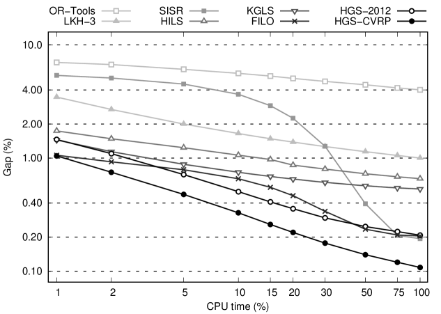
Figure 4: Convergence of the algorithms over time

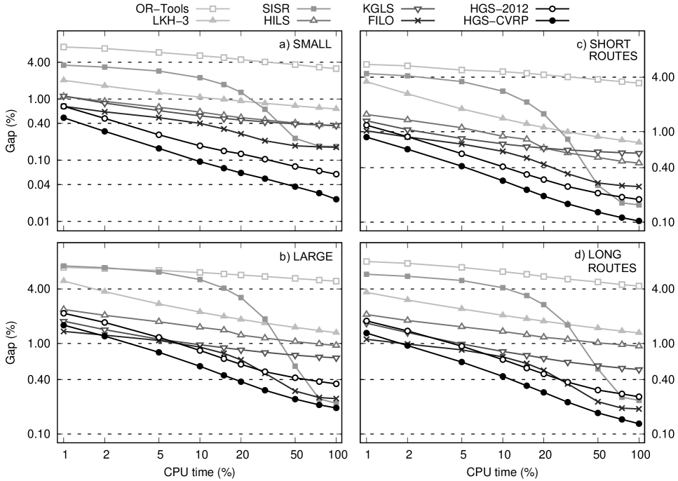
Figure 5: Convergence of the algorithms over time for different subgroups of instances

As visible in Figures 4–5, the relative rank of the algorithms in terms of solution quality remains generally stable over time, except for SISR which converges towards high-quality solutions only later in the run. This behavior is due to its simulated-annealing acceptance criterion (with an exponential temperature decay), which favors exploration during the earlier phases of the search and only triggers convergence when the temperature is low enough. We observe that HGS-CVRP outperforms HGS-2012 and the other algorithms at any point in time (from 1% to 100%) and that Swap* positively impacts the search even at early stages. KGLS finds good quality solutions in general, but it does not converge faster than other approaches as initially claimed. HILS performs better on instances with short routes, due to the increased effectiveness of its set-partitioning component in that regime. Finally, SISR and FILO achieve their peak performance on larger instances, confirming the observations of the authors.

Analysis of the SWAP* neighborhood. To conclude our analysis, Figure 6 displays the share of the computational time dedicated to the exploration of each neighborhood (Relocate and variants thereof involving consecutive node pairs, Swap and variants thereof involving consecutive node pairs, 2-Opt, 2-Opt*, and Swap*), as well as the relative proportion of moves of each type applied during the first loop of the local search (the first time these moves are tried for a given solution) and during the rest of the local search (once the most “obvious” local search moves have been already applied). These figures are based on run statistics collected during ten executions on six instances with diverse characteristics from the extended “sensitivity analysis” benchmark of Uchoa et al. (2017). The characteristics of these instances are summarized in Table 7, in which $r$ represents the expected number of customers in the routes.

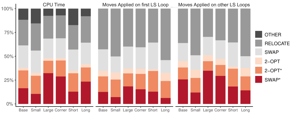
Figure 6: Statistics on the use of the neighborhoods of HGS-CVRP

Table 7: Characteristics of the instances used in the sensitivity analysis

Instance	$n$	Depot	$r$
Base	200	Centered	[9,11]
Small	100	Centered	[9,11]
Large	600	Centered	[9,11]
Corner	200	Corner	[9,11]
Short	200	Centered	[3,5]
Long	200	Centered	[21,22]

As visible in Figure 6, the share of the computational time of HGS-CVRP dedicated to the exploration of the Swap* neighborhood does not exceed 32%, confirming the effectiveness of the proposed exploration and move filtering strategies which permit to limit the complexity of this neighborhood search. This is a significant achievement, given that this neighborhood is much larger than classic neighborhoods (e.g., Relocate or Swap). According to our experiments, Swap* is responsible for approximately 15% of the solution improvements. It also produces a larger proportion of improvements at later stages of the local search, when it is more difficult to find improving moves.

Some instance characteristics directly impact the performance of the neighborhoods. Instances with a larger number of customers or a depot location in the corner have proportionally more Swap* moves due to the proposed move filtering strategy. Consequently, the CPU time consumption and the number of applied moves tend to be higher in these situations. The Swap* neighborhood is also more effective when the routes contain fewer customers on average, as it finds a larger share of improvements in a smaller computational effort in proportion. Indeed, improving Swap* moves often correspond to pairs of Relocate moves that are individually improving but infeasible due to capacity limits, a recurrent case when optimizing many short routes.

6 Conclusions

This paper helped to fulfill two important goals: 1) facilitating future research by providing a simple, state-of-the-art code base for the CVRP; and 2) introducing a neighborhood called Swap* along with pruning and exploration strategies that permit an efficient search in a time similar to smaller neighborhoods such as Swap, Relocate or 2-Opt*. We conducted an extensive computational campaign to compare the convergence of the proposed HGS-CVRP algorithm with that of the original HGS (Vidal et al. 2012) and other algorithms provided to us by their authors, using the same computational platform. These analyses demonstrate that HGS-CVRP stands as the leading metaheuristic in terms of solution quality and convergence speed while remaining conceptually simple. As visible in these results, Swap* largely contribute to the search performance, especially at later stages of the local searches when improving moves are more difficult to find.

For future research, we recommend pursuing general research on the complexity of neighborhood explorations. For the CVRP, we can indeed argue that recent improvements in heuristic solution methods are due to more efficient and focused local searches rather than new metaheuristic concepts. Moreover, new breakthroughs are still being regularly made on the theoretical aspects of neighborhood search (see, e.g., De Berg et al. 2021). We also insist on the role of simplification in experimental design and scientific reasoning. While revisiting HGS and specializing it to the CVRP, we did systematic tests to retain only the most essential elements. Indeed, solution quality gains can almost always be achieved at the cost of having a method that is more convoluted and difficult to reproduce. Certainly, HGS-CVRP could be improved by dedicating a small fraction of its search effort into an additional set-partitioning component, additional decomposition phases, or mutation steps inspired by ruin-and-recreate. Nevertheless, we refrained from pushing further in that direction yet, as the goal of heuristic design should be to 1) identify methodological concepts that are as simple and effective as possible, and 2) to properly understand the role of each component. Therefore, we hope that the release of HGS-CVRP will contribute towards a general better understanding of heuristics for difficult combinatorial optimization problems.

References

- Accorsi and Vigo (2021) Accorsi, L., D. Vigo. 2021. A fast and scalable heuristic for the solution of large-scale capacitated vehicle routing problems. Transportation Science 55(4) 832–856.
- Aiex et al. (2007) Aiex, R.M., M.G.C. Resende, C.C. Ribeiro. 2007. TTT plots: A Perl program to create time-to-target plots. Optimization Letters 1(4) 355–366.
- Arnold and Sörensen (2018) Arnold, F., K. Sörensen. 2018. What makes a VRP solution good? The generation of problem-specific knowledge for heuristics. Computers & Operations Research 106 280–288.
- Beasley (1983) Beasley, J.E. 1983. Route first-cluster second methods for vehicle routing. Omega 11(4) 403–408.
- Christiaens and Vanden Berghe (2020) Christiaens, J., G. Vanden Berghe. 2020. Slack induction by string removals for vehicle routing problems. Transportation Science 54(2) 299–564.
- De Berg et al. (2021) De Berg, M., K. Buchin, B.M.P. Jansen, G. Woeginger. 2021. Fine-grained complexity analysis of two classic TSP variants. ACM Transactions on Algorithms. 17(1) 1–29.
- Glover and Hao (2011) Glover, F., J.-K. Hao. 2011. The case for strategic oscillation. Annals of Operations Research 183(1) 163–173.
- Guillen et al. (2020) Guillen, F.O., M. Gendreau, J.-Y. Potvin, T. Vidal. 2020. A ruin & recreate ant colony system algorithm for the capacitated vehicle routing problem. Working Paper. CIRRELT.
- Helsgaun (2017) Helsgaun, K. 2017. An extension of the Lin-Kernighan-Helsgaun TSP solver for constrained traveling salesman and vehicle routing problems. Technical Report, Roskilde University.
- Kendall et al. (2016) Kendall, G., R. Bai, J. Błazewicz, P. De Causmaecker, M. Gendreau, R. John, J. Li, B. McCollum, E. Pesch, R. Qu, N. Sabar, G. Vanden Berghe, A. Yee. 2016. Good laboratory practice for optimization research. Journal of the Operational Research Society 67 676–689.
- Laporte et al. (2014) Laporte, G., S. Ropke, T. Vidal. 2014. Heuristics for the vehicle routing problem. P. Toth, D. Vigo, eds., Vehicle Routing: Problems, Methods, and Applications, chap. 4. Society for Industrial and Applied Mathematics, 87–116.
- Moscato and Cotta (2010) Moscato, P., C. Cotta. 2010. A modern introduction to memetic algorithms. M. Gendreau, J.-Y. Potvin, eds., Handbook of Metaheuristics, vol. 146. Springer, New York, 141–183.
- Oliver et al. (1987) Oliver, I., D. Smith, J.R. Holland. 1987. A study of permutation crossover operators on the traveling salesman problem. J. Grefenstette, ed., Genetic Algorithms and their Applications: Proceedings of the Second International Conference. 224–230.
- Prins (2004) Prins, C. 2004. A simple and effective evolutionary algorithm for the vehicle routing problem. Computers & Operations Research 31(12) 1985–2002.
- Subramanian et al. (2013) Subramanian, A., E. Uchoa, L.S. Ochi. 2013. A hybrid algorithm for a class of vehicle routing problems. Computers & Operations Research 40(10) 2519–2531.
- Talbi (2009) Talbi, El Ghazali. 2009. Metaheuristics: From Design to Implementation. John Wiley & Sons.
- Toth and Vigo (2014) Toth, P., D. Vigo, eds. 2014. Vehicle Routing: Problems, Methods, and Applications. 2nd ed. Society for Industrial and Applied Mathematics, Philadelphia.
- Uchoa et al. (2017) Uchoa, E., D. Pecin, A. Pessoa, M. Poggi, A. Subramanian, T. Vidal. 2017. New benchmark instances for the capacitated vehicle routing problem. European Journal of Operational Research 257(3) 845–858.
- Vidal (2016) Vidal, T. 2016. Technical note: Split algorithm in O(n) for the capacitated vehicle routing problem. Computers & Operations Research 69 40–47.
- Vidal (2017) Vidal, T. 2017. Node, edge, arc routing and turn penalties: Multiple problems – One neighborhood extension. Operations Research 65(4) 992–1010.
- Vidal et al. (2012) Vidal, T., T.G. Crainic, M. Gendreau, N. Lahrichi, W. Rei. 2012. A hybrid genetic algorithm for multidepot and periodic vehicle routing problems. Operations Research 60(3) 611–624.
- Vidal et al. (2014) Vidal, T., T.G. Crainic, M. Gendreau, C. Prins. 2014. A unified solution framework for multi-attribute vehicle routing problems. European Journal of Operational Research 234(3) 658–673.
- Vidal et al. (2015) Vidal, T., T.G. Crainic, M. Gendreau, C. Prins. 2015. Time-window relaxations in vehicle routing heuristics. Journal of Heuristics 21(3) 329–358.
- Vidal et al. (2020) Vidal, T., G. Laporte, P. Matl. 2020. A concise guide to existing and emerging vehicle routing problem variants. European Journal of Operational Research 286 401–416.
- Vidal et al. (2016) Vidal, T., N. Maculan, L.S. Ochi, P.H.V. Penna. 2016. Large neighborhoods with implicit customer selection for vehicle routing problems with profits. Transportation Science 50(2) 720–734.
- Vidal et al. (2021) Vidal, T., R. Martinelli, T.A. Pham, M.H. Hà. 2021. Arc routing with time-dependent travel times and paths. Transportation Science 55(3) 706–724.
- Zachariadis and Kiranoudis (2010) Zachariadis, E.E., C.T. Kiranoudis. 2010. A strategy for reducing the computational complexity of local search-based methods for the vehicle routing problem. Computers & Operations Research 37(12) 2089–2105.