The Cosmic-Ray Composition between 2 PeV and 2 EeV Observed with the TALE Detector in Monocular Mode

Abstract

We report on a measurement of the cosmic ray composition by the Telescope Array Low-Energy Extension (TALE) air fluorescence detector (FD). By making use of the Cherenkov light signal in addition to air fluorescence light from cosmic ray (CR) induced extensive air showers, the TALE FD can measure the properties of the cosmic rays with energies as low as $\sim 2$ PeV and exceeding 1 EeV. In this paper, we present results on the measurement of $X_{\rm max}$ distributions of showers observed over this energy range. Data collected over a period of $\sim 4$ years was analyzed for this study. The resulting $X_{\rm max}$ distributions are compared to the Monte Carlo (MC) simulated data distributions for primary cosmic rays with varying composition and a 4-component fit is performed. The comparison and fit are performed for energy bins, of width 0.1 or 0.2 in $\log_{10}(E/{\rm eV})$, spanning the full range of the measured energies. We also examine the mean $X_{\rm max}$ value as a function of energy for cosmic rays with energies greater than $10^{15.8}$ eV. Below $10^{17.3}$ eV, the slope of the mean $X_{\rm max}$ as a function of energy (the elongation rate) for the data is significantly smaller than that of all elements in the models, indicating that the composition is becoming heavier with energy in this energy range. This is consistent with a rigidity-dependent cutoff of events from galactic sources. Finally, an increase in the $X_{\rm max}$ elongation rate is observed at energies just above $10^{17}$ eV indicating another change in the cosmic rays composition.

1 Introduction

The TALE detector was designed to look for structure in the energy spectrum and associated change in composition of cosmic rays below the “ankle” structure at $10^{18.6}$ eV. A measurement of the cosmic ray energy spectrum using TALE observations in the energy range between $10^{15.3}$ eV and $10^{18.3}$ eV was published in a recent article (Abbasi et al., 2018a). Here we present our results on the cosmic ray composition from $10^{15.3}$ eV to $10^{18.3}$ eV. Only the high elevation telescopes of TALE observing $31^{\circ}$ to $55^{\circ}$, are used in this analysis. See section 2 for the experimental setup.

Previous observations of cosmic rays composition for energies greater than $10^{18}$ eV, such as those reported by HiRes (Abbasi et al., 2005), the Telescope Array (TA) (Abbasi et al., 2015), and Auger (Aloisio et al., 2014), all suggest that the transition from galactic to extragalactic sources occurs at an energy below that of the ankle. This transition is expected to be observable in the form of a composition getting heavier up to a “transition energy” and then becoming lighter at higher energies. Below the transition energy, galactic sources dominate the observed flux, while above the transition the sources of cosmic rays are mostly extragalactic.

Several observations of the cosmic ray energy spectrum, including the one using TALE data, indicate the presence of a “knee”-like structure in the $10^{17}$ decade, a second knee. A change in the spectral index of the cosmic ray flux is also expected in the case of transition from galactic to extragalactic sources. It is therefore logical to expect to see a correlated change in the flux and composition in the transition region. This paper reports on the observation of just such a correlated change.

We describe the detector and data collection in section 2. We then briefly discuss event selection and event reconstruction procedures in section 3. In section 4 we describe the Monte Carlo (MC) simulation, and present the results of MC studies of the event reconstruction performance. Section 5 presents an overview of the composition measurement procedures. A discussion of the systematic uncertainties is presented in section 6. The measured composition is shown in section 7, along with a brief discussion of the measured results. The paper concludes with a summary in section 8.

As the second paper on TALE data analysis, it is unavoidable that some of the material presented in this paper reproduces already published material in (Abbasi et al., 2018a). Furthermore, we refer the reader to that publication for a more detailed description of the TALE detector and data analysis.

2 TALE Detector and Operation

The Telescope Array is an international collaboration with members from Japan, U.S., South Korea, Russia, and Belgium. The observatory is located in the West Desert of Utah, about 150 miles southwest of Salt Lake City, and is the largest cosmic ray detector in the northern hemisphere. In operation since 2008, TA consists of 507 scintillator surface detectors (SD), arranged in a square grid of 1.2 km spacing (Abu-Zayyad et al., 2013a). A total of 38 telescopes are distributed among three FD stations located on the periphery of the SD array (Abu-Zayyad et al., 2012; Tokuno et al., 2012). The FD telescopes observe the airspace above the SD array. TA is the direct successor to both the Akeno Giant Air Shower Array (AGASA) and the High Resolution Fly’s Eye (HiRes) experiments (Teshima et al., 1986; Sokolsky, 2011). Telescope Array incorporates both the scintillation counter technique of AGASA and the air fluorescence measurements of HiRes. The goal of the Telescope Array is to clarify the origin and nature of ultra-high energy cosmic rays (UHECR) and the related extremely high energy phenomena in the universe. The previous measurements of the energy spectrum, composition, and anisotropy in the arrival direction distribution for energies above $10^{18.2}$ eV have been published (Abu-Zayyad et al., 2013b; Abbasi et al., 2015, 2014)

A TA Low-Energy extension (TALE) fluorescence detector (Thomson et al., 2011) began operation in 2013 at the northern FD station (Middle Drum). Ten new TALE telescopes were added to the 14 telescopes which made up the TA FD at the site. All 24 telescopes were refurbished from components previously used by HiRes, and updated with new communications hardware. The original 14 TA FD telescopes came from HiRes-I and were distributed in two “rings” viewing $3^{\circ}$ to $31^{\circ}$ in elevation. They are instrumented with Sample-and-Hold electronics. The TALE FD telescopes, added to TA in 2013, came from HiRes-II and view $31^{\circ}$ to $59^{\circ}$ in elevation, directly above the field of view of the main Telescope Array Telescopes. The TALE telescopes are instrumented with FADC electronics.

In addition to the ten new, high-elevation angle, FD telescopes, TALE also added 103 new SD counters arranged in a graded spacing array. See Figure 1. Both the TA and TALE telescopes view approximately southeast, over the Telescope Array and TALE SD arrays. This arrangement is illustrated in Figure 2.

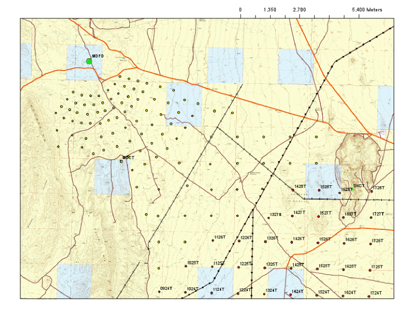
Figure 1: Map of the TALE detector. The locations of the TALE surface detectors is indicated by the yellow circles. The TALE detectors merge with the main Telescope Array surface array at the lower right of the figure. Telescope Array surface detectors are shown by red circles with detector numbers. The location of the TALE FD site can be seen near the top left of the figure indicated on the map by the green hexagon labeled MDFD

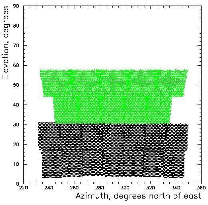
Figure 2: Schematic of TALE/MD telescopes field of view, showing azimuthal and elevation coverage. Each small hexagon represents the field of view of a single PMT, while the broad box outlines show the field of view of a 256 PMT telescope camera. The view of the 14 TA telescopes is shown in black, while that of the 10 TALE telescopes is shown in green.

The TALE scintillator detectors were added after the telescopes in 2017. Since the telescopes were taking data before the scintillators were deployed, the analysis described in this paper is based only upon observations made by the FD component of TALE.

The TALE FD telescopes were assembled from refurbished HiRes-II telescopes (Boyer et al., 2002). The telescope mirrors are each made from four truncated circular segments which were assembled into a clover-leaf pattern. The unobscured viewing area of each spherical mirror is approximately $3.7$ m². The focal plane of the telescope camera consists of 256 (16x16) hexagonal photo-multiplier tubes (PMTs). The Philips/Photonis XP3062 PMTs are 40-mm (flat-to-flat) where each PMT/pixel views a $1^{\circ}$ cone in the sky. The field-of-view (FOV) of each camera is about $16^{\circ}$ in azimuth by $14^{\circ}$ in elevation.

The TALE telescope electronics consist of a 10 MHz FADC readout system with 8-bit resolution. Analog sums over the rows and columns of pixels, also sampled at 8-bits, allow recovery of saturated PMTs in most cases. The trigger logic of the telescope also uses the digitized summed signals. Systems for telescope GPS timing, inter-telescope triggers and communication to a central data acquisition (DAQ) computer use new hardware that resulted in a significant improvement in throughput over the old HiRes-II system, and are documented in  (Zundel, 2016).

Useful events recorded by the TALE detector appear as tracks for which the observed signal is comprised of a combination of direct Cherenkov light (CL) and fluorescence light (FL), with some contribution from scattered CL. Contributions of light generated by these mechanisms are both proportional to the number of charged particles in the extensive air shower (EAS) at any point along its development. Thus, CL signals can be analyzed in a manner analogous to that for FL to determine the energy of the cosmic ray, as well as to determine the depth of shower maximum ($X_{\rm max}$) which is related to the composition of the primary particle.

There are some important differences between the CL and FL measurements. First, FL is emitted isotropically along the shower from the particles. In contrast, the CL is strongly peaked in the forward direction along the shower axis. As a result, CL falls off rapidly as the incident angle of the shower to the detector increases. In addition, the CL also accumulates along the shower track and therefore increases in overall intensity as the shower develops. Both types of light also undergo scattering in the atmosphere, from both air molecules (Rayleigh scattering) as well as from particulate aerosols.

At the lowest energies observable by TALE, events are dominated by CL. At higher energies, however, the FD becomes more sensitive to the isotropically emitted FL. In the energy region between $10^{16.5}$eV and $10^{17.5}$eV, the shower events are typically recorded with a mix of both CL and FL. Based upon our experience with the TALE energy spectrum calculation, we concluded that a composition analysis, which requires accurate reconstruction of the shower geometry, should be restricted to use only those events with a significant contribution of direct CL. Therefore, we restrict our analysis to events with direct CL $>35\%$ of the total recorded signal; see Section 3 and Table 2 of (Abbasi et al., 2018a).

TALE FD data collected between June 2014 and November 2018 is included in this analysis. This data set includes, as a subset, the data set used for the energy spectrum paper (Abbasi et al., 2018a). However, this data set is more than double the size of the original spectrum data set. The criteria used for good-weather determination is the same as in the original analysis. The total, good-weather, detector on-time in this period is $\sim$ 2700 hours.

3 Event Processing and Reconstruction

Most TALE FD data events are the result of noise triggers or very low-energy air showers that can not be reliably used for physics analysis. An event processing chain is used that filters out low quality events. After filtering, the remaining events are subjected to full shower reconstruction, which includes the determination of shower geometry, energy, and the depth of shower maximum.

The event reconstruction procedure consists of the following main steps:

First, the shower-detector plane (SDP) is reconstructed from the pattern and pointing direction of the triggered PMT pixels.

Next, the arrival time of light at the detector (in each pixel) is fit as a function of the viewing angle of the pixel in the SDP:

$$t_{i}=t_{0}+\frac{R_{p}}{c}\tan\left(\frac{\pi-\psi-\chi_{i}}{2}\right),$$ (1)

where $R_{p}$ is the impact parameter or distance of closest approach from the detector to the shower track, $\psi$ is the incline angle of the track within the SDP, $t_{0}$ is a time offset, and $\chi_{i}$ is the viewing angle of the i-th pixel.

The PMT signal is then fit to the light profile expected for a given energy and shower $X_{\rm max}$ according to the Gaisser-Hillas parameterization:

The parametrization gives the number of charged particles, $N$, at atmospheric depth, $x$, along the shower track. $N_{\rm max}$, $X_{\rm max}$, $X_{0}$, and $\lambda$ are parameters. Here, $N_{\rm max}$ is the number of shower particles at the point of maximum shower development, $X_{\rm max}$. $X_{0}$ is a fit parameter roughly indicating the starting depth of the shower and $\lambda=70$ g/cm². In combination with $X_{0}$, $\lambda$ sets the width of the shower profile curve. The fit produces two numbers of interest: $X_{\rm max}$, the depth of shower maximum development and the shower’s calorimetric energy. The calculation of the total shower energy follows from the fit results, as explained below.

Table 1: Quality cuts applied to events used for the composition measurement. Events meeting these conditions remain in the analysis.

Variable	CL
Angular Track-length [deg]	$trk>6.1^{\circ}$
Inverse Angular Speed [$\mu$s deg-1]	$0.014<1/\omega<0.1$
Shower Impact Parameter [km]	$0.4<R_{p}<5.0$
Shower Zenith Angle [deg]	$28^{\circ}<\theta<65^{\circ}$
Shower $X_{\rm max}$ [g cm-2]	$435<X_{\rm max}<920$
Estimated Fit Error on Energy	$\delta E/E<0.6$
Estimated Fit Error on $X_{\rm max}$ [g cm-2]	$\delta X_{\rm max}<200$
Timing Fit $\chi^{2}/dof$	$\chi^{2}_{tim}<4.5$
Profile Fit $\chi^{2}/dof$	$\chi^{2}_{pfl}<12$

The profile constrained geometry fit (PCGF) (AbuZayyad, 2000) was used to reconstruct this TALE data. When applied to TALE events with a significant CL signal, we found that the PCGF results in very good geometry resolutions (Abbasi et al., 2018a). Based upon MC studies, we determined that a direct CL fraction of at least 35% was optimal for maintaining good geometrical reconstruction and at the same time increasing event statistics at higher energies, approaching $10^{18}$ eV.

The PCGF reconstruction produces an estimate for the shower calorimetric energy. To obtain the total shower energy, i.e. the primary CR particle energy, a missing energy correction is applied. This correction is composition dependent, and is therefore applied after the best fit composition parameters have been determined. We refer to the primary mixture obtained from fitting TALE data as “TXF”, for TALE $\bm{X}_{max}$ distributions Fits, see Section 5. Post-reconstruction, event selection criteria (quality cuts) are summarized in Table 1.

4 Simulation

We use Monte Carlo simulations to study the detector efficiency and reconstruction resolution. Two sets of simulations were generated for this analysis using different hadronic interaction models. The first set of simulations was based upon QGSJetII-03 (Ostapchenko, 2007) and a second set was based upon EPOS-LHC (Pierog et al., 2015). QGSjetII-03 is the model that was previously used for the TALE energy spectrum measurement (Abbasi et al., 2018a), while the EPOS-LHC model is a “post-LHC” model, i.e. a hadronic interaction model that has been updated with LHC data.

The full processing of a set of simulations is a time consuming process. This made it unfeasible for us to perform the full analysis using other, post-LHC, hadronic interaction models, such as QGSJetII-04 (Ostapchenko, 2011). We do note, however, that a comparison of CONEX (Bergmann et al., 2007) simulations in the energy range of interest for this publication, shows that the air shower’s $\langle X_{\rm max}\rangle$ predictions of QGSJetII-03 are within 5.0 g/cm² of the QGSJetII-04 model for all of the four primaries used in this analysis, as demonstrated in Figure 3.

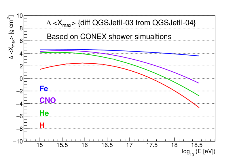
Figure 3: Difference in mean $X_{\rm max}$ predictions for the QGSjetII-03 and QGSjetII-04 hadronic interaction models. The difference between the mean shower maximum in showers generated using QGSjetII-03 versus those using QGSJetII-04 is shown as a function of energy for four different cosmic ray primaries: H, He, CNO, and Fe. The shower simulations were generated using CONEX.

For both sets of simulations, with the QGSjetII-03 and EPOS-LHC hadronic interaction models, a uniform mixture of four primaries {H, He, N, Fe} was simulated for the energy range of 10¹⁵ - 10^18.5 eV. The showers were thrown following a power law flux with a spectral index of -2.92. The MC shower events were then re-weighted to fit a broken power law spectrum consistent with the TALE energy spectrum measurement.

A detailed simulation of the TALE detector response to cosmic ray generated air showers is performed. For each hadronic interaction model, a library of air showers generated using the CONEX package is used as input to the detector MC. Light production by shower particles and light propagation to the detector, including accurate photon arrival time determination, is performed. This is followed by a detailed simulation of the detector optics and electronics signal development, and finally by detector trigger and event forming logic simulation.

The MC is generated for each data collection time interval that the TALE telescope station was operated. Nightly atmospheric conditions (three hour interval GDAS (ARL-NOAA, 2004) database), and nightly detector calibration information is incorporated into the simulation. Each MC data set is about twice size of the actual data set.

Figure 4: Reconstruction resolution of the shower angle in the shower-detector plane, $\psi$. The red curve is a Gaussian fit to the distribution of the uncertainty, $\Delta\psi$ [deg]. Distribution statistics are displayed in top-right box. The MC uses the EPOS-LHC hadronic generator and a mixed composition, matching the TXF results. From left to right, the histograms show the distribution of the uncertainty, $\Delta\psi$ [deg], for events reconstructed in three energy ranges: $10^{15.3}$ - $10^{16.3}$ eV, $10^{16.3}$ - $10^{17.3}$ eV, and $10^{17.3}$ - $10^{18.3}$ eV. The resolution of the shower angle, $\psi$, along with the resolution of the impact parameter, $R_{p}$, determines the accuracy of the shower track reconstruction.

Figure 5: Reconstruction resolution of the shower impact parameter, $R_{p}$. The red curve is a Gaussian fit to the distribution of the fractional uncertainty, $\Delta R_{p}/R_{p}$. Distribution statistics are displayed in top-right box. The MC uses the EPOS-LHC hadronic generator and a mixed composition, matching the TXF results. From left to right, the histograms show the distribution of the fractional uncertainty, $\Delta R_{p}/R_{p}$, for events reconstructed in three energy ranges: $10^{15.3}$ - $10^{16.3}$ eV, $10^{16.3}$ - $10^{17.3}$ eV, and $10^{17.3}$ - $10^{18.3}$ eV. As can be seen, the resolution improves significantly with energy.

Figure 6: Reconstruction resolution of shower maximum, $X_{\rm max}$. The red curve is a Gaussian fit to the distribution of the uncertainty, $\Delta X_{max}~{}[{\rm g~{}cm}^{-2}]$. Distribution statistics are displayed in top-right box. The MC uses the EPOS-LHC hadronic generator and a mixed composition, matching the TXF results. From left to right, the histograms show the distribution of the the uncertainty, $\Delta X_{max}~{}[{\rm g~{}cm}^{-2}]$, for events reconstructed in different energy ranges: $10^{15.3}$ - $10^{16.3}$ eV, $10^{16.3}$ - $10^{17.3}$ eV, and $10^{17.3}$ - $10^{18.3}$ eV.

Figure 7: Reconstruction resolution of the shower energy, $E$. The red curve is a Gaussian fit to the distribution of the fractional uncertainty, $\Delta E/E$. Distribution statistics are displayed in top-right box. The MC uses the EPOS-LHC hadronic generator and a mixed composition, matching the TXF results. From left to right, the histograms show the distribution of the fractional uncertainty, $\Delta E/E$, for events reconstructed in three energy ranges: $10^{15.3}$ - $10^{16.3}$ eV, $10^{16.3}$ - $10^{17.3}$ eV, and $10^{17.3}$ - $10^{18.3}$ eV.

Simulated MC showers pass through the same event selection criteria as the real data and they are reconstructed using the same program/procedure. A missing energy correction is applied to both the reconstructed data and MC showers based on the same composition assumption, with the correction for each primary type and energy being estimated from the CONEX generated showers.

Here, the cosmic rays composition is described by the fit fractions of the various primaries obtained in this study. The fitting procedure uses the measured calorimetric energy of the showers. After the fit fractions are calculated, this information is incorporated into the analysis scripts to estimate the total shower energy for each event as a weighted average over the four primaries used in the simulations, with the fit fractions as weights.

We next present event reconstruction performance, namely resolution and bias of reconstructed shower parameters. The most relevant shower parameters are:

1. The angle in the shower-detector plane, $\psi$

2. The shower impact parameter to the detector, $R_{p}$

3. The depth of shower maximum, $X_{\rm max}$, and

4. The shower energy, $E$.

The first set of results is shown for all MC showers, i.e. four primaries. The same number of showers were generated for each primary, but the detection and reconstruction efficiencies are different for each primary and therefore the final number of showers is different. Note that, the results shown here use the EPOS-LHC simulation set. The results using the QGSJetII-3 hadronic generator are similar.

Figures 4 - 7 show the difference between the reconstructed and thrown values of simulated events, i.e. the reconstruction resolution of the shower parameters. In light of the steeply falling number of events with energy, each figure is shown as three separate plots, one per energy decade.

As can be seen from the figures, the reconstruction performance improves with energy. The $\psi$ resolution for the three energy ranges is $1.1^{\circ}$, $0.83^{\circ}$, and $0.67^{\circ}$. The impact parameter fractional error, $dR_{p}/R_{p}$, expressed as a percent is 7.5%, 3.5%, and 2.0%. The $X_{\rm max}$ resolution averaged over the four primaries is 47, 40, and 31 g cm^-2. In all cases, the bias in the reconstruction is small compared to the resolution. Figure 7 shows the resolutions for the reconstructed energy, $dE/E$. The energy resolutions are 17%, 11%, and 9% for the three energy bins. For the full range of the data set, we see negligible bias in the reconstructed energy values. Note that the energy estimate here includes the missing energy correction.

Figure 8: Shower $X_{\rm max}$, reconstruction resolution. The histograms (blue) show the uncertainty, $\Delta X_{max}~{}[{\rm g~{}cm}^{-2}]$ for MC events reconstructed in three different energy ranges; from the left to right: (a) $10^{15.3}$ - $10^{16.3}$ eV, (b) $10^{16.3}$ - $10^{17.3}$ eV, and (c) $10^{17.3}$ - $10^{18.3}$ eV. The red curve represents a Gaussian fit to the histogram. The distributions are shown for each of the four simulated primaries, from top to bottom: (1) H, (2) He, (3) N, (4) Fe.

The second set of results is shown for individual CR primaries. Here we only show the $X_{\rm max}$ results, (see Figure 8), since this is the only variable that shows any significant variance for the different primaries. The total shower energy will, naturally, be biased since we use an average missing energy correction. As can be seen from Figure 8, the $X_{\rm max}$ resolution has similar magnitude and improves with energy for each type of primary. The reconstruction bias, however, shows a dependence on primary type; as can be seen by looking at the means of the distributions in Figure 8. At lower energies, we see that $X_{\rm max}$ is underestimated for the lighter primaries, and overestimated for heavier primaries. The difference in bias among the different primaries decreases with energy.

As a further check on the shower reconstruction performance, we tested an alternative detector response simulation procedure. We replaced the calculation of shower Cherenkov photons reaching the TALE detector, performed by our usual MC program, with a procedure using CORSIKA with the IACT package (Bernlohr, 2008). Photons generated by CORSIKA are “injected” into the simulated detector at the times and into the pixels predicted by the IACT package. This is an independent calculation from the one used in the reconstruction and can serve to test the validity of the Cherenkov light modeling used in event reconstruction, as well as, to verify our estimates for the shower reconstruction performance. A study using the two detector simulation procedures showed good agreement between the estimates of the detector acceptance ($\sim 10\%$), and reconstruction performance: energy ($\sim 5\%$), $X_{\rm max}$ ($\sim 10~{}{\rm g~{}cm}^{-2}$), when using identical sets of CORSIKA showers. The same reconstruction procedure was applied to both sets. The reader is referred to (Abbasi et al., 2018a) for more details on this study.

5 Composition Analysis

We examine both the mean depth of shower maximum, $\langle X_{\rm max}\rangle$, as well as the full $X_{\rm max}$ distribution in order to study the composition of cosmic rays. The mean depth of shower maximum is known to depend upon the cosmic ray primary type. Therefore, the change of the mean $X_{\rm max}$ with energy, the elongation rate, can be examined for indications of a change in composition, e.g. evolution from a heavy to a light composition or vice versa. Comparison of the mean $X_{\rm max}$ to that of MC showers of different primary types allow for the inference of the dominant (if any) primary in the measured flux.

Note that the detector acceptance and event selection and reconstruction biases result in a primary mixture in the final data set that is different from the true mixture, at the top of the atmosphere. Therefore, the interpretation of the results can only be made by comparison to MC generated showers. The reconstructed MC showers are subject to the same biases as the real showers.

The analysis fits the full $X_{\rm max}$ distribution histogram of the observed data to the weighted sum of four histograms of reconstructed MC showers, one for each simulated primary type. The result of the fit is a set of weights (fit fractions) that are used to produce a combined MC histogram, as a weighted sum of the four primary MC histograms, that best matches the data histogram. The fractions are corrected for the detector acceptance of each primary, using the known MC event counts, to produce fractions which are independent of the detector acceptance.

The fit procedure starts by binning the reconstructed events in energy using a bin size of 0.1 in $\log_{10}(E_{cal}/{\rm eV})$, where $E_{cal}$ is the reconstructed calorimetric shower energy. This is the energy estimate obtained from the fit to the PMT signals, and is independent of primary type. In each energy bin, the data and MC $X_{\rm max}$ distributions are histogramed with a bin size of 10 g cm^-2. The fit is performed by calculating a weighted sum of the four MC histograms representing the reconstructed $X_{\rm max}$ distributions of the four primaries (Filthaut, 2002; Barlow & Beeston, 1993). A “true fraction” is then determined taking into account the relative detection and reconstruction efficiencies for each primary type.

Figure 9: Shower $X_{\rm max}$ (g/cm²) distributions for energy bin $15.2<\log_{10}(E_{cal}/{\rm eV})<15.3$. Each of four plots shows data histogram (black points / blue line), along with MC primary reconstructed $X_{\rm max}$: upper left plot H (red), upper right He (green), lower left CNO (violet), and lower right Fe (blue)

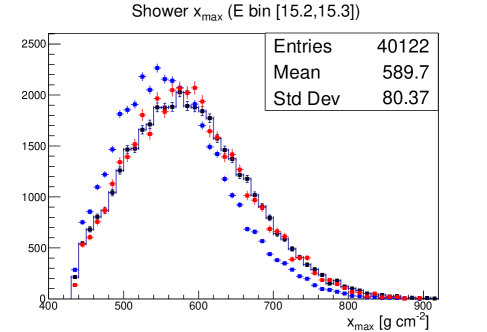
Figure 10: Shower $X_{\rm max}$ (g/cm²) distributions for energy bin $15.2<\log_{10}(E_{cal}/{\rm eV})<15.3$. Black points represent the data, the $X_{\rm max}$ distribution fit result (TXF) is shown in red. Using the H4a (Gaisser, 2012) composition model as input to the TALE detector MC results in the distribution shown in blue.

As is well known from shower simulations, there is significant overlap in the $X_{\rm max}$ distributions obtained from different cosmic ray primary particles with the same energy. A practical consequence of this fact is that attempts to fit a measured distribution using MC generated distributions do not benefit from including many primaries in the fit. On the contrary, the fit becomes unstable, and gives results with highly correlated fit parameters, i.e. primary fractions, making the physical interpretation of the results difficult. For this reason, we chose to use only four primaries for this analysis, namely H, He, N (CNO), and Fe that cover the range of interest. An example of the measured $X_{\rm max}$ distributions, and MC primary reconstructed $X_{\rm max}$ distributions in the same energy bin, $15.2<\log_{10}(E_{cal}/{\rm eV})<15.3$, is shown in Figure 9. We find that that the choice of four primaries is sufficient to provide a good fit to the data at all energies. This is shown in Figure 10 for the same energy bin. The figure also shows the reconstructed $X_{\rm max}$ distribution that results from using the H4a (Gaisser, 2012) composition model as input to the TALE detector simulation.

6 Systematic Uncertainties

The main sources of systematic uncertainties on the $\langle X_{\rm max}\rangle$ measurement are the energy scale uncertainty and possible uncertainty in the detector acceptance calculations in the MC. The main source of uncertainty in the cosmic ray composition measurement, i.e. primary fractions estimates, comes from the selection of hadronic model used in the shower simulations.

The TALE detector total energy scale uncertainty was estimated to be $\pm$15%, including a $\pm$10% contribution from the shower missing energy correction (Abbasi et al., 2018a). This implies that the uncertainty on the reconstructed shower calorimetric energy is $\sim 10\%$. To estimate the systematic uncertainty on the fit to the primary fractions and quantities derived from them, we propagate the uncertainty in the calorimetric energy, as explained below.

Systematic uncertainty due to detector acceptance effects are investigated below, however, they are not folded into the final systematic uncertainty. This is due to the fact that some of contributions are small enough to be ignored, while others are contained within the calorimetric energy uncertainty and are therefore already accounted for.

The choice of hadronic model determines the predicted $X_{\rm max}$ distribution for each of the primary particles which are used to fit the data $X_{\rm max}$ distributions. To a first approximation, we can consider the differences in the predictions of each hadronic model for the mean value of $X_{\rm max}$ of each primary as a measure of the systematic uncertainty introduced by the choice of a particular model. An examination of the shower simulations using various post-LHC models (Pierog, 2018) has shown that the predictions of the different models for the mean $X_{\rm max}$ lie in an interval of about 20 g cm^-2, with EPOS-LHC producing results in the middle of those predicted by QGSJetII-04 and Sybil2.3-c (Engel et al., 2017). We therefore, estimate the uncertainty on the $\langle X_{\rm max}\rangle$ of simulated CR primaries to be $\pm~{}10~{}{\rm g~{}cm}^{-2}$ around those used in our EPOS-LHC MC set.

The data analysis was also performed using the QGSJetII-03 model, producing an equivalent set of results which can be compared to the results using EPOS-LHC. A comparison of the results using the two models includes the effects not only of differences in the $\langle X_{\rm max}\rangle$, but the full $X_{\rm max}$ distributions. In addition, the comparison introduces a shift in the energy scale due to the different missing energy correction.

The systematic uncertainty on the $\langle X_{\rm max}\rangle$ measurements was calculated by shifting the reconstructed event (total) energy by $\pm~{}15\%$, while also shifting the reconstructed event $X_{\rm max}$ by $\pm~{}10~{}{\rm g~{}cm}^{-2}$. The $\pm$ sign in both shifts is chosen to move the $\langle X_{\rm max}\rangle$ versus energy in the same direction. The $\pm~{}10~{}{\rm g~{}cm}^{-2}$ in this case is attributed to detector acceptance bias, and to reconstruction bias introduced by Cherenkov light modeling (Abbasi et al., 2018a).

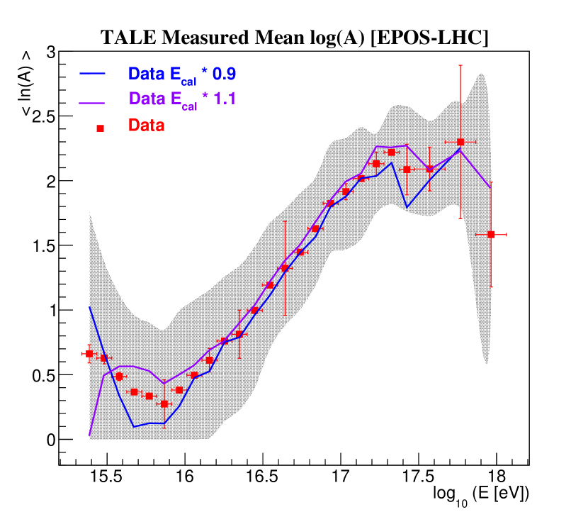
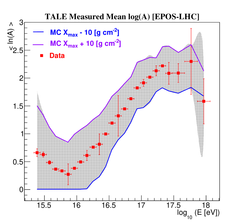
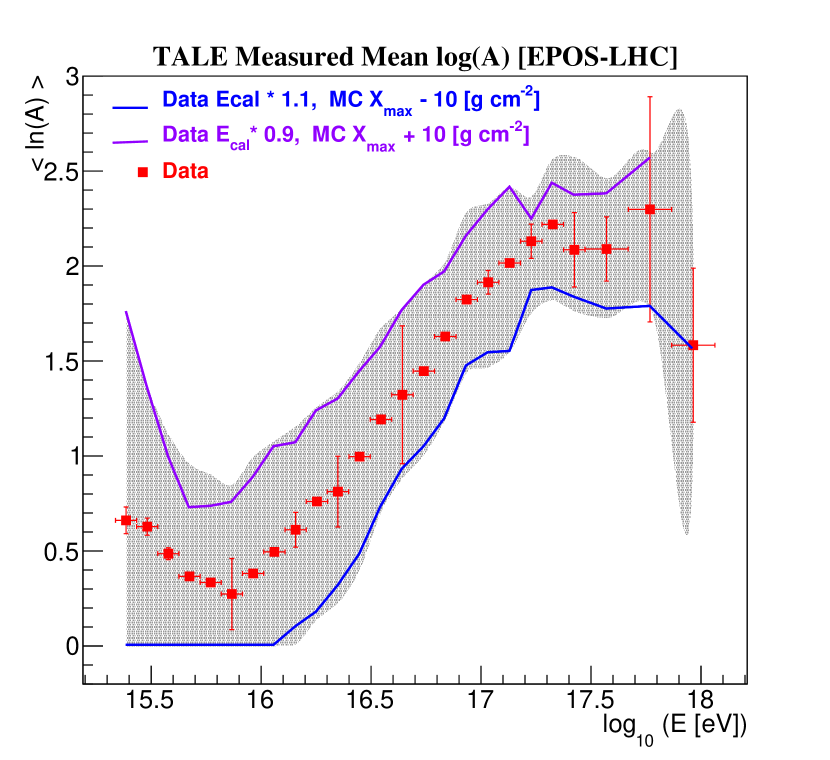
Figure 11: The $\langle\ln(A)\rangle$ systematics band (shown in gray) compared to the effect on the estimated $\langle\ln(A)\rangle$ of shifting the reconstructed data events energy by $\pm 10\%$ (top), or shifting reconstructed $X_{\rm max}$ values of MC showers by $\pm 10~{}{\rm g~{}cm}^{-2}$ (middle), or the combination of the two (bottom). In all three panels, points with error bars are TALE data with no systematic shifts to event energy or MC showers $X_{\rm max}$.

The systematics bands displayed in the primary fractions obtained by fitting the data $X_{\rm max}$ distributions were calculated by repeating the fitting procedure with some variations: (1) Shift the calorimetric energy of the data by $\pm~{}10\%$. (2) Shift the MC $X_{\rm max}$ distributions by $\pm~{}10~{}{\rm g~{}cm}^{-2}$, a common shift is applied for the four components. (3) Combine these shifts when they have an additive effect on the resulting shift in the fit fractions for the different primaries. We examined six different sets of fits and set the bounds on each primary fraction at the minimum and maximum values obtained by any of the six shifted sets.

We can summarize a set of four fit-fractions as a single number using the definition: $\langle\ln(A)\rangle=\sum_{ip}{f_{ip}*\ln(A_{ip})}$ where $ip$ stands for one of {H, He, N, Fe}. In the following discussion, we use this quantity to examine the overall systematic uncertainty of the composition measurement. We start with Figure 11, showing the six different combinations of energy and $X_{\rm max}$ shifts, discussed above, along with the overall systematics band.

To estimate the size of the uncertainty due to acceptance, we divide the data into multiple subsets and redo the analysis on these subsets. We also vary some of the event quality cuts values and examine how the results change with these modifications.

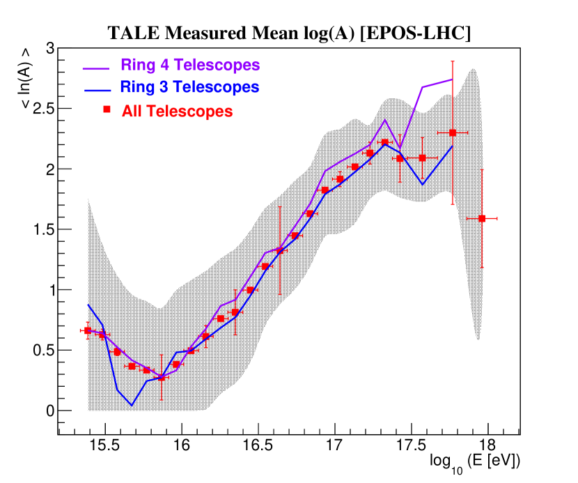
Figure 12: The $\langle\ln(A)\rangle$ for the full TALE dataset compared to subsets using Ring 3 (31-45^∘ elevation) and Ring 4 (45-59^∘ elevation) events separately. For most of the energy range, the difference between the two subsets is small relative to other systematics. Near the bottom and top of the energy range the difference is comparable to other systematics.

The vast majority of the events in the final data set are single telescope events. Thus, a possible way to create subsets of the data is to divide the set by telescope. “Ring 4” telescopes view higher elevation angles (45-59^∘ elevation), therefore, they are more likely to trigger on heavy primaries, due to shorter path through the atmosphere, than “Ring 3” telescopes (viewing 31-45^∘ elevation). Division by telescope “ring” is related to division by shower zenith angle, since Cherenkov dominated events must have a direction that is close to the pointing angle of the observing telescope. The comparison of the two is shown in Figure 12. As can be seen in the figure, the difference between the two subsets is small relative to other systematics for most of the energy range. Near the ends of the energy range the difference is comparable to other systematics.

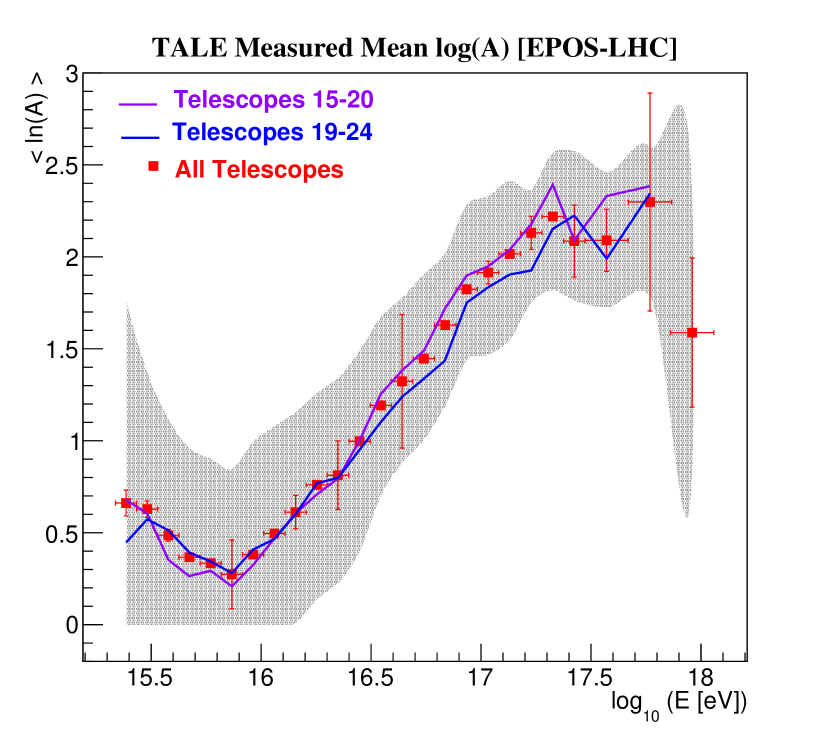
Figure 13: The $\langle\ln(A)\rangle$ for the full TALE dataset compared to subsets using telescopes with different azimuthal viewing directions. Telescopes 15-20 point farther east, while 19-24 point farther west; two telescopes 19, 20 are shared by the two subsets. As can be seen in the plot, there is a relatively small azimuthal effect at higher energies, but it is not a major contributor to the overall systematic uncertainty.

An east, west division of telescopes with the central two telescopes included in both sets, checks for any geomagnetic effect and different sky noise background. Results of a comparison are shown in Figure 13. As can be seen in the figure, there is a relatively small azimuthal effect at higher energies, but it is not a major contributor to the overall systematic uncertainty.

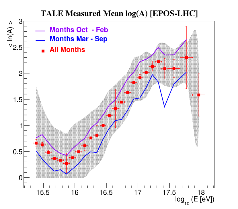
Figure 14: The $\langle\ln(A)\rangle$ for the full TALE dataset compared to subsets using “winter” months October through February and the months of March through September. This break down gives similar number of events in each subset. Despite the use of hourly GDAS atmospheric pressure profiles in the simulation and event reconstruction, we still find a significant difference in the predictions based on season.

Another source of uncertainty on detector acceptance are time dependent effects such as atmospheric clarity or sky noise background that may not be accurately reflected in the detector simulation. To examine these effects, we divide the data in time, namely in time of year. Winter months usually allow for longer run periods, and so we divided the data into a set collected during the months of October through February, and another from March through September. This division showed the largest difference in the absolute value of $\langle\ln(A)\rangle$ of all the various checks we performed. The comparison is shown in Figure 14. Despite the use of hourly GDAS atmospheric pressure profiles in the simulation and event reconstruction, we still find a significant difference in the predictions based on season.

A possible cause for the difference is, the seasonal variation in the average concentration of atmospheric aerosols. The nightly, or even hourly, density of aerosols is variable, and difficult to measure continuously. It can be treated on average however. For the TALE analysis, an average concentration characterized by the vertical aerosols optical depth, VAOD, is used. Aerosols attenuate the light signal reaching the detector from the shower. Therefore, a variation in the aerosols concentration results in a variation in the amount of light reaching the detector from the shower. An increase in the light attenuation can cause some showers to either fail to trigger the detector, or otherwise, to pass some reconstruction or quality cut. Summer months in Utah tend to have poorer air quality, i.e. more aerosols, and therefore more light attenuation. Showers created by heavier primaries, larger $\ln(A)$, develop higher up in the atmosphere, and light produced by these showers will travel further in the atmosphere, through more aerosols, to reach the detector. We speculate that the effect of increased average aerosols concentration will be stronger for heavier primaries than light primaries, resulting in a decrease of the fraction of heavy primaries in the data and therefore a smaller $\langle\ln(A)\rangle$. This is the observed effect for TALE, as can be seen in Figure 14.

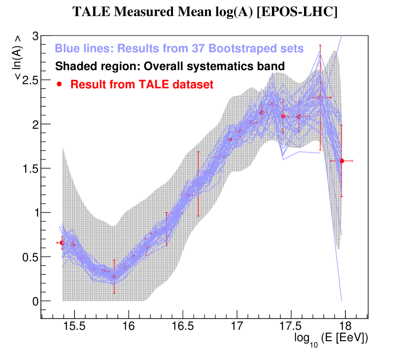
Figure 15: The $\langle\ln(A)\rangle$ for the full TALE dataset compared to 37 artificial sets generated using the bootstrap method, with sampling over run months (58 months in total). By randomly sampling the run months we get a measure of the overall effect of atmospheric variation on the composition result. We see that, when averaged over the entire data set, the effect of atmospheric variations on the composition result is likely smaller than the expectation based on the seasons check, shown in Figure 14.

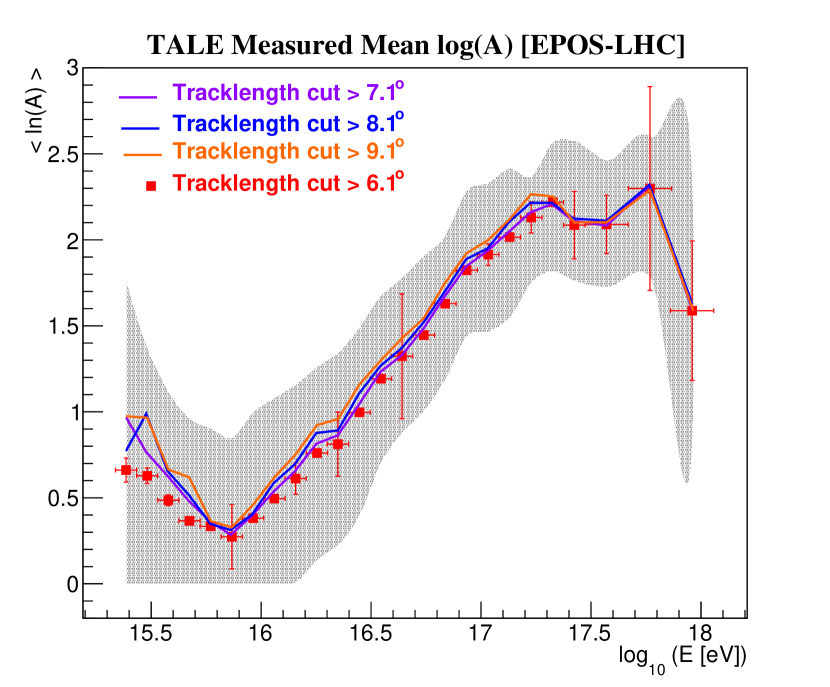
Figure 16: The $\langle\ln(A)\rangle$ for TALE data using standard quality cuts compared to changes of cut value on the event angular-tracklength. As can be seen, changing the track-length cut has a minimal effect on the composition results. Similar results were observed for other cut parameters examined as part of the data analysis.

Another approach to look at time dependence of the result is to use the Bootstrap method (Efron, 1979), to sample different run months and form a data set comparable to the actual set in terms of the number of events. The complete observation period is comprised of 58 run months. By sampling run months instead of individual events, we maintain the correspondence between the simulation and real data included in the sampled set. We performed 37 iterations to obtain a measure of the stability of the result and to get a sense of the expected spread of the result due to inclusion or exclusion of certain run periods. Results are shown in Figure 15. By randomly sampling the run months we get a measure of the overall effect of atmospheric variation on the composition result. We see that, when averaged over the entire data set, the effect of atmospheric variations on the composition result is likely smaller than the expectation based on the seasons check, shown in Figure 14.

Finally, we examined varying some of the quality cuts applied to the data and simulation sets. As an example, the effect of changing the cut value of the angular track-length is shown in Figure 16. As can be seen in the figure, changing the track-length cut has a minimal effect on the composition results. Similar results were observed for other cut parameters examined as part of the data analysis.

7 Results and Discussion

We present the results of the analysis in the following forms:

1. Measured $\langle X_{\rm max}\rangle$ evolution with shower energy. These values are for the final event sample and do not include corrections for detector acceptance bias or other biases related to event selection or event reconstruction. We also show the results for reconstructed MC showers for comparison with the data.

2. Estimated cosmic ray primary fractions based on the full measured $X_{\rm max}$ distribution, using a four component fit. The primary fractions in this case are corrected for biases in detector acceptance, event selection, and event reconstruction.

3. Resulting $\langle\ln(A)\rangle$ from the bias corrected four component fit. This result can be thought of as a condensed form of the four component fit result.

4. Bias corrected $X_{\rm max}$ using EPOS-LHC fit fractions and the unbiased EPOS-LHC MC prediction for the mean $X_{\rm max}$ of the four primary particles used in the analysis.

Where applicable, the above results are shown separately for the two hadronic models, QGSJetII-03 and EPOS-LHC.

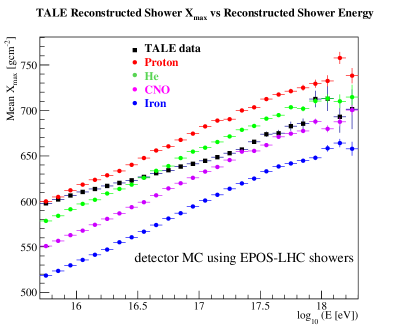
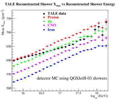
Figure 17: Mean $X_{\rm max}$ as a function of energy for the reconstructed TALE events. Shower missing energy correction estimate using EPOS-LHC is shown in the upper plot, and using QGSJetII-03 in the lower plot. The reconstructed $X_{\rm max}$ values for the four MC primaries, generated and reconstructed using the corresponding hadronic model, are shown alongside the data for comparison. The data appears to be getting heavier with energy in this range for both models.

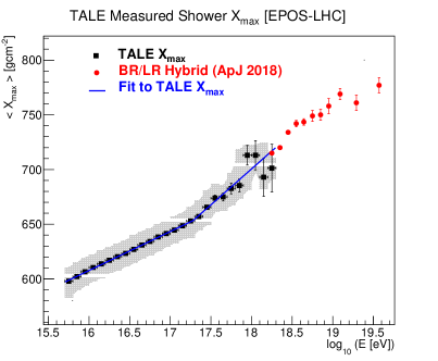
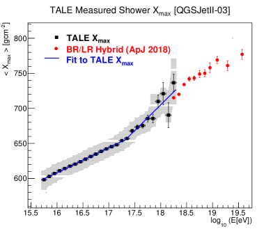
Figure 18: Mean $X_{\rm max}$ as a function of energy for the reconstructed TALE events. Shower missing energy correction estimate using EPOS-LHC is shown in the upper plot, and using QGSJetII-03 lower plot. A broken line fit is shown for each plot. Fit parameters are listed in Table 2. Red points at higher energies come from a hybrid measurement by the main Telescope Array telescopes (Abbasi et al., 2018b).

Figure 17 shows the mean $X_{\rm max}$ values of TALE data along with those of simulated showers. At $\sim 10^{18}$, it can be seen that the event statistics becomes low. The data is presented in Tables 3, 4 in Appendix A.

Table 2: Fit parameters to a broken line fit to TALE $X_{\rm max}$ elongation rate: The upper set of measurements are for the EPOS-LHC, the lower set is for QGSJetII-03.

EPOS-	break point	17.291 $\pm 0.060+0.077-0.084$
LHC	slope before	35.863 $\pm 0.294+1.481-0.536$
	slope after	65.413 $\pm 6.655+0.000-3.269$
QGSJet-	break point	17.310 $\pm 0.049+0.052-0.179$
II-03	slope before	35.784 $\pm 0.298+1.337-0.667$
	slope after	70.860 $\pm 6.508+0.000-11.387$

The elongation rate at energies below $10^{17.3}$ eV indicates that the composition is getting heavier in this energy range. A change in the elongation rate (slope of the line fit to $X_{\rm max}$ vs energy) is clearly seen for energies greater than $10^{17}$ eV that is not present in the MC showers for any one primary type. This change in slope can be interpreted as a change in composition. A broken line fit (one floating break point) to the slope is used to determine the energy at which the slope changes. The fit is shown in Figure 18; Fit results are presented in Table 2. The fit line is in agreement with the mean $X_{\rm max}$ values measured by the Telescope Array detectors at EeV energies (Abbasi et al., 2018b), as can be seen in Figure 18.

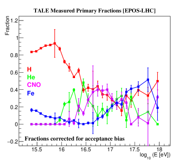
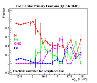
Figure 19: Fit results to the data $X_{\rm max}$ distributions (per energy bin) to a four component MC distributions. Primary fractions using the EPOS-LHC based simulations are shown in the top plot. Those using QGSJetII-03, in the bottom plot.

Figure 20: Primary fractions using the EPOS-LHC based simulations are shown for a four primary composition.

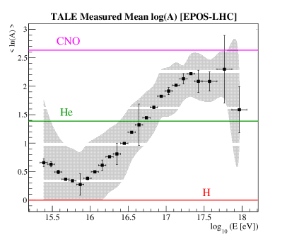
Figure 21: Estimated $\langle\ln(A)\rangle$ from four component fits to TALE data. Horizontal lines show calculated $\ln(A)$ values for H, He, and N, for reference.

Data $X_{\rm max}$ distributions were created for each energy bin, using a bin width of 0.1 in $\log_{10}(E)$ up to an energy of $10^{17.4}$ eV, then 0.2 in $\log{E}$ up to $10^{18}$ eV. These distributions were fit using MC distributions created using either of two hadronic interaction models, and containing four different primaries. Fit results are shown in Figure 19. The small number of observed events with energies greater than $10^{18}$ eV was not sufficient to extend the fits beyond $10^{18}$ eV.

To incorporate the systematic uncertainty into the presentation of the results we focus our attention on the EPOS-LHC based analysis. The primary fractions are shown separately in Figure 20, followed by the estimated $\langle\ln(A)\rangle$ displayed in Figure 21. Similar to the trend found for $\langle X_{\rm max}\rangle$, figures 20 and 21 also indicate that the composition is getting heavier in the $10^{16}$ eV decade, and that there is a further change just above $10^{17}$ eV.

Finally, similar to the calculation of $\langle\ln(A)\rangle$, the bias corrected fractions were used to calculate a no-bias $\langle X_{\rm max}\rangle=\sum_{ip}{f_{ip}*\langle X^{(ip)}_{\rm max}\rangle}$, where $ip$ stands for one of {H, He, N, Fe}, and $\langle X^{(ip)}_{\rm max}\rangle$ is the EPOS-LHC predicted (MC thrown) $\langle X_{\rm max}\rangle$ of primary $ip$. These results are displayed in Figure 22, with data in Table 5.

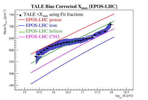
Figure 22: Bias corrected $X_{\rm max}$ using EPOS-LHC fit fractions and the unbiased EPOS-LHC MC prediction for the mean $X_{\rm max}$ of the four primary particles used in the analysis. These results include a first order correction to the detector acceptance bias.

8 Summary

We presented the results of a measurement of the cosmic rays composition in the energy range of $10^{15.3}$ - $10^{18.3}$ eV using data collected by the TALE detector over a period of roughly four years. An examination of the mean $X_{\rm max}$ versus energy, (Figures 17, 18), shows a composition that is getting heavier, followed by a change in the $X_{\rm max}$ elongation rate at an energy of $\sim 10^{17.3}$ eV. This “break” in the elongation rate is likely correlated with the observed break in the cosmic rays energy spectrum (Abbasi et al., 2018a).

We also fit the data $X_{\rm max}$ distributions, per energy bin, to reconstructed MC showers generated for four primary particle types. These fits show a light mostly proton and Helium composition at the lower energies becoming more mixed near $10^{17}$ eV. In this analysis, we do not have sufficient statistics to comment on the composition for cosmic rays with energies greater than $10^{18}$ eV. These results are shown as the fractions themselves, Figures 19, 20, as a derived mean $\ln(A)$, Figure 21, and a derived mean $X_{\rm max}$, Figure 22.

Software

Appendix A

Mean shower $X_{\rm max}$ for events included in the composition analysis of TALE data are shown in Tables 3 and  4. The number of events in each energy bin, along with the $X_{\rm max}$ and estimated errors are listed. Table 5 lists the bias corrected $\langle X_{\rm max}\rangle$ of data events, estimated using the bias corrected fit fractions from EPOS-LHC based analysis.

Table 3: $\langle X_{\rm max}\rangle$ of data events. Missing energy correction based on EPOS-LHC hadronic model.

energy-bin	Number	$\langle X_{\rm max}\rangle\pm\sigma_{stat.}+/-\sigma_{sys.}$
log10 (E [eV])	of Events	g cm-2
15.30-15.40	39669	590.1 $\pm$ 0.4 + 10.0 - 10.0
15.40-15.50	71699	585.8 $\pm$ 0.3 + 10.0 - 10.0
15.50-15.60	98113	585.8 $\pm$ 0.3 + 12.4 - 10.5
15.60-15.70	109055	589.8 $\pm$ 0.2 + 15.6 - 12.8
15.70-15.80	97017	597.9 $\pm$ 0.3 + 13.0 - 14.9
15.80-15.90	91380	602.1 $\pm$ 0.3 + 12.8 - 12.6
15.90-16.00	78444	606.4 $\pm$ 0.3 + 13.2 - 12.7
16.00-16.10	64594	610.4 $\pm$ 0.3 + 12.0 - 12.2
16.10-16.20	51230	613.6 $\pm$ 0.3 + 12.7 - 12.2
16.20-16.30	40036	617.0 $\pm$ 0.4 + 12.2 - 11.5
16.30-16.40	30915	620.3 $\pm$ 0.4 + 12.1 - 12.5
16.40-16.50	23657	623.2 $\pm$ 0.4 + 12.4 - 11.7
16.50-16.60	17972	626.9 $\pm$ 0.5 + 13.1 - 12.2
16.60-16.70	13517	630.9 $\pm$ 0.6 + 12.7 - 12.2
16.70-16.80	9940	634.2 $\pm$ 0.6 + 12.2 - 12.1
16.80-16.90	7644	638.3 $\pm$ 0.7 + 11.8 - 12.8
16.90-17.00	5560	641.3 $\pm$ 0.8 + 12.8 - 11.9
17.00-17.10	4284	644.5 $\pm$ 1.0 + 12.9 - 11.5
17.10-17.20	3059	648.6 $\pm$ 1.1 + 12.0 - 12.2
17.20-17.30	1833	653.0 $\pm$ 1.4 + 12.8 - 14.8
17.30-17.40	1295	657.0 $\pm$ 1.8 + 14.8 - 12.4
17.40-17.50	807	665.5 $\pm$ 2.2 + 15.1 - 15.9
17.50-17.60	487	673.8 $\pm$ 2.9 + 13.4 - 12.5
17.60-17.70	300	674.9 $\pm$ 3.6 + 10.6 - 11.9
17.70-17.80	176	682.7 $\pm$ 4.9 + 14.0 - 15.6
17.80-17.90	112	685.4 $\pm$ 5.7 + 33.4 - 12.0
17.90-18.00	57	712.5 $\pm$ 9.0 + 10.0 - 31.4
18.00-18.10	25	712.8 $\pm$ 13.4 + 10.0 - 14.8
18.10-18.20	16	692.9 $\pm$ 17.4 + 32.2 - 10.0
18.20-18.30	5	701.3 $\pm$ 21.8 + 10.0 - 10.0

Table 4: $\langle X_{\rm max}\rangle$ of data events. Missing energy correction based on QGSJetII-03 hadronic model.

energy-bin	Number	$\langle X_{\rm max}\rangle\pm\sigma_{stat.}+/-\sigma_{sys.}$
log10 (E [eV])	of Events	g cm-2
15.30-15.40	43977	589.3 $\pm$ 0.4 + 10.0 - 10.0
15.40-15.50	75692	585.6 $\pm$ 0.3 + 10.0 - 10.0
15.50-15.60	100698	586.1 $\pm$ 0.3 + 13.0 - 10.8
15.60-15.70	109617	590.8 $\pm$ 0.2 + 15.3 - 13.3
15.70-15.80	96990	598.2 $\pm$ 0.3 + 13.3 - 14.4
15.80-15.90	89810	602.8 $\pm$ 0.3 + 12.8 - 12.6
15.90-16.00	76271	607.0 $\pm$ 0.3 + 13.2 - 12.9
16.00-16.10	62828	610.8 $\pm$ 0.3 + 12.1 - 11.8
16.10-16.20	49683	614.1 $\pm$ 0.3 + 12.4 - 12.5
16.20-16.30	38534	617.4 $\pm$ 0.4 + 12.1 - 11.4
16.30-16.40	29904	620.4 $\pm$ 0.4 + 12.5 - 11.8
16.40-16.50	22732	623.8 $\pm$ 0.4 + 12.1 - 12.1
16.50-16.60	17201	627.3 $\pm$ 0.5 + 13.2 - 12.4
16.60-16.70	13166	631.3 $\pm$ 0.6 + 12.5 - 11.7
16.70-16.80	9447	634.7 $\pm$ 0.7 + 12.7 - 12.3
16.80-16.90	7338	638.6 $\pm$ 0.8 + 11.8 - 12.4
16.90-17.00	5389	642.0 $\pm$ 0.9 + 12.8 - 12.6
17.00-17.10	4075	645.3 $\pm$ 1.0 + 11.4 - 12.4
17.10-17.20	2916	648.0 $\pm$ 1.1 + 14.2 - 10.8
17.20-17.30	1719	653.9 $\pm$ 1.5 + 13.0 - 14.3
17.30-17.40	1241	657.0 $\pm$ 1.8 + 16.4 - 12.3
17.40-17.50	762	667.8 $\pm$ 2.4 + 12.6 - 17.5
17.50-17.60	450	673.1 $\pm$ 3.0 + 13.2 - 11.8
17.60-17.70	285	675.4 $\pm$ 3.6 + 15.5 - 10.8
17.70-17.80	167	685.5 $\pm$ 4.9 + 10.0 - 18.5
17.80-17.90	107	685.5 $\pm$ 6.1 + 35.0 - 10.9
17.90-18.00	50	709.8 $\pm$ 9.2 + 10.0 - 22.7
18.00-18.10	20	719.9 $\pm$ 15.9 + 10.0 - 25.6
18.10-18.20	16	690.4 $\pm$ 18.0 + 35.0 - 10.0
18.20-18.30	5	736.5 $\pm$ 12.3 + 35.0 - 30.4

Table 5: Bias corrected $\langle X_{\rm max}\rangle$ of data events, estimated using the bias corrected fit fractions from EPOS-LHC based analysis. Statistical uncertainties are those on the mean of the corresponding measured data histogram bin. Systematics are calculated based on estimated systematic uncertainties on primary fit fractions.

energy-bin	Number	$\langle X_{\rm max}\rangle\pm\sigma_{stat.}+/-\sigma_{sys.}$
log10 (E [eV])	of Events	g cm-2
15.338-15.434	40122	572.5 $\pm$ 0.4 + 20.4 - 34.0
15.434-15.530	70340	579.6 $\pm$ 0.3 + 19.2 - 22.6
15.530-15.626	94914	590.1 $\pm$ 0.3 + 14.7 - 19.0
15.626-15.723	105576	599.8 $\pm$ 0.2 + 11.0 - 17.7
15.723-15.819	95197	606.8 $\pm$ 0.3 + 9.9 - 16.8
15.819-15.915	90591	614.7 $\pm$ 0.3 + 8.0 - 16.6
15.915-16.012	78786	617.7 $\pm$ 0.3 + 10.9 - 17.1
16.012-16.109	65331	621.2 $\pm$ 0.3 + 13.3 - 16.3
16.109-16.205	52467	624.2 $\pm$ 0.3 + 15.9 - 15.3
16.205-16.302	41031	626.5 $\pm$ 0.3 + 16.2 - 14.1
16.302-16.399	31743	630.8 $\pm$ 0.4 + 15.6 - 14.8
16.399-16.496	24609	632.7 $\pm$ 0.4 + 15.3 - 13.9
16.496-16.594	18644	633.0 $\pm$ 0.5 + 13.4 - 13.3
16.594-16.691	14051	635.5 $\pm$ 0.6 + 12.2 - 12.6
16.691-16.788	10544	637.9 $\pm$ 0.6 + 12.5 - 12.4
16.788-16.886	7920	639.4 $\pm$ 0.7 + 12.0 - 11.0
16.886-16.984	5919	640.1 $\pm$ 0.8 + 10.6 - 12.0
16.984-17.081	4485	644.0 $\pm$ 0.9 + 11.9 - 11.0
17.081-17.179	3259	647.6 $\pm$ 1.1 + 11.9 - 10.8
17.179-17.277	2031	651.0 $\pm$ 1.3 + 10.1 - 7.0
17.277-17.375	1377	653.8 $\pm$ 1.7 + 10.3 - 9.1
17.375-17.473	904	663.6 $\pm$ 2.1 + 8.7 - 11.9
17.473-17.670	896	672.1 $\pm$ 2.1 + 9.1 - 9.6
17.670-17.866	331	678.7 $\pm$ 3.4 + 12.3 - 7.8
17.866-18.063	110	708.2 $\pm$ 6.5 + 12.5 - 12.5

References

- Aartsen et al. (2017) Aartsen, M., et al. 2017, JINST, 12, P03012, doi: 10.1088/1748-0221/12/03/P03012
- Aartsen et al. (2019) —. 2019, Phys. Rev. D, 100, 082002, doi: 10.1103/PhysRevD.100.082002
- Abbasi et al. (2013) Abbasi, R., et al. 2013, Nucl. Instrum. Meth. A, 700, 188, doi: 10.1016/j.nima.2012.10.067
- Abbasi et al. (2005) Abbasi, R. U., et al. 2005, Astrophys. J., 622, 910, doi: 10.1086/427931
- Abbasi et al. (2014) —. 2014, Astrophys. J., 790, L21, doi: 10.1088/2041-8205/790/2/L21
- Abbasi et al. (2015) —. 2015, Astropart. Phys., 64, 49, doi: 10.1016/j.astropartphys.2014.11.004
- Abbasi et al. (2018a) —. 2018a, Astrophys. J., 865, 74, doi: 10.3847/1538-4357/aada05
- Abbasi et al. (2018b) —. 2018b, Astrophys. J., 858, 76, doi: 10.3847/1538-4357/aabad7
- Abu-Zayyad et al. (2012) Abu-Zayyad, T., et al. 2012, Astropart. Phys., 39-40, 109, doi: 10.1016/j.astropartphys.2012.05.012
- Abu-Zayyad et al. (2013a) —. 2013a, Nucl. Instrum. Meth., A689, 87, doi: 10.1016/j.nima.2012.05.079
- Abu-Zayyad et al. (2013b) —. 2013b, Astrophys. J., 768, L1, doi: 10.1088/2041-8205/768/1/L1
- AbuZayyad (2000) AbuZayyad, T. Z. 2000, PhD thesis, Utah U. http://www.telescopearray.org/media/papers/tareq_thesis.pdf
- Aloisio et al. (2014) Aloisio, R., Berezinsky, V., & Blasi, P. 2014, JCAP, 1410, 020, doi: 10.1088/1475-7516/2014/10/020
- Antoni et al. (2003) Antoni, T., et al. 2003, Nucl. Instrum. Meth. A, 513, 490, doi: 10.1016/S0168-9002(03)02076-X
- Antoni et al. (2005) —. 2005, Astropart. Phys., 24, 1, doi: 10.1016/j.astropartphys.2005.04.001
- ARL-NOAA (2004) ARL-NOAA. 2004, http://ready.arl.noaa.gov/gdas1.php
- Barlow & Beeston (1993) Barlow, R. J., & Beeston, C. 1993, Comput. Phys. Commun., 77, 219, doi: 10.1016/0010-4655(93)90005-W
- Bergmann et al. (2007) Bergmann, T., Engel, R., Heck, D., et al. 2007, Astropart. Phys., 26, 420, doi: 10.1016/j.astropartphys.2006.08.005
- Bernlohr (2008) Bernlohr, K. 2008, Astropart.Phys., 30, 149, doi: 10.1016/j.astropartphys.2008.07.009
- Boyer et al. (2002) Boyer, J. H., Knapp, B. C., Mannel, E. J., & Seman, M. 2002, Nucl. Instrum. Meth., A482, 457, doi: 10.1016/S0168-9002(01)01517-0
- Efron (1979) Efron, B. 1979, Ann. Statist., 7, 1, doi: 10.1214/aos/1176344552
- Engel et al. (2017) Engel, R., Riehn, F., Fedynitch, A., Gaisser, T. K., & Stanev, T. 2017, EPJ Web Conf., 145, 08001, doi: 10.1051/epjconf/201614508001
- Filthaut (2002) Filthaut, F. 2002, https://root.cern/doc/master/classTFractionFitter.html
- Gaisser (2012) Gaisser, T. K. 2012, Astropart. Phys., 35, 801, doi: 10.1016/j.astropartphys.2012.02.010
- Heck et al. (1998) Heck, D., Schatz, G., Thouw, T., Knapp, J., & Capdevielle, J. N. 1998
- Ostapchenko (2007) Ostapchenko, S. 2007, AIP Conf. Proc., 928, 118, doi: 10.1063/1.2775904
- Ostapchenko (2011) —. 2011, Phys. Rev. D, 83, 014018, doi: 10.1103/PhysRevD.83.014018
- Peters (1961) Peters, B. 1961, 22, 800
- Pierog (2018) Pierog, T. 2018, PoS, ICRC2017, 1100, doi: 10.22323/1.301.1100
- Pierog et al. (2015) Pierog, T., Karpenko, I., Katzy, J. M., Yatsenko, E., & Werner, K. 2015, Phys. Rev., C92, 034906, doi: 10.1103/PhysRevC.92.034906
- Sokolsky (2011) Sokolsky, P. 2011, Nucl. Phys. Proc. Suppl., 212-213, 74, doi: 10.1016/j.nuclphysbps.2011.03.010
- Teshima et al. (1986) Teshima, M., et al. 1986, Nucl. Instrum. Meth., A247, 399, doi: 10.1016/0168-9002(86)91324-0
- Thomson et al. (2011) Thomson, G., Sokolsky, P., Jui, C., et al. 2011, The telescope array low energy extension (TALE), Vol. 3 (Institute of High Energy Physics), 337–339
- Tokuno et al. (2012) Tokuno, H., et al. 2012, Nucl. Instrum. Meth., A676, 54, doi: 10.1016/j.nima.2012.02.044
- Yoon et al. (2017) Yoon, Y., et al. 2017, Astrophys. J., 839, 5, doi: 10.3847/1538-4357/aa68e4
- Zundel (2016) Zundel, Z. J. 2016, PhD thesis, University of Utah