Diffusion Limits at Small Times for Coalescent Processes with Mutation and Selection

Abstract

The Ancestral Selection Graph (ASG) is an important genealogical process which extends the well-known Kingman coalescent to incorporate natural selection. We show that the number of lineages of the ASG with and without mutation is asymptotic to $2/t$ as $t\to 0$, in agreement with the limiting behaviour of the Kingman coalescent. We couple these processes on the same probability space using a Poisson random measure construction that allows us to precisely compare their hitting times. These comparisons enable us to characterise the speed of coming down from infinity of the ASG as well as its fluctuations in a functional central limit theorem. This extends similar results for the Kingman coalescent.

, , and

1 Introduction and Main Results

The Kingman coalescent [1] is one of the fundamental models in the field of population genetics, though it has many mathematical qualities that are of independent interest. If one takes a large population of individuals and considers their ancestry into the past, a process that models the structure of this ancestry is the Kingman coalescent. Mathematically it is characterised as a continuous-time Markov process over the space of partitions of $\mathbb{N}=\{1,2,3,\dots\}$, where each pair of blocks in the partition coalesces independently at unit rate; each block representing an ancestral lineage.

This process can be initialised from the partition of singletons $\{\{1\},\{2\},\dots\}$, in which case the associated block-counting process $(N^{0,0}_{t})_{t\geq 0}$ starts at $+\infty$ and instantly becomes finite almost surely [2]. This phenomenon is called “coming down from infinity” and motivates investigation into the behaviour of $N^{0,0}_{t}$ close to $t=0$.

In [3] Griffiths derives asymptotic expressions for $N^{0,0}_{t}$ when $t$ is small. There it is shown that, as $t\to 0$, $N^{0,0}_{t}$ is approximately Gaussian with mean $2/t$ and variance $2/(3t)$. These approximations are often used when simulating the Wright-Fisher diffusion [4].

When considering the “coming down from infinity” behaviour of the coalescent, a natural question to ask is how quickly this happens. Specifically, one looks for a function $\nu_{t}$ such that

$$\lim_{t\to 0}\frac{N^{0,0}_{t}}{\nu_{t}}=1,~{}~{}a.s.$$ (1)

In [5] it is proved that for those general birth/death processes which come down from infinity, one can define $\nu$ as

$$\nu_{t}:=\inf\{n\geq 0;~{}\mathbb{E}_{\infty}[T_{n}]\leq t\},$$ (2)

where $T_{n}$ is the hitting time of $n$ and the subscript on $\mathbb{E}$ denotes that the process started from infinity. For the Kingman coalescent a known function satisfying (1) is $2/t$ [2, Theorem 4.9]. It should be noted that any function which satisfies $\nu_{t}\sim 2/t$ as $t\to 0$ will also satisfy (1).

In [6] the authors fully characterised the fluctuations of $N^{0,0}_{t}$ as $t\to 0$ by proving the convergence of

$$X^{0,0}_{\varepsilon}(t):=\varepsilon^{-1/2}\left(\frac{\varepsilon t}{2}N^{0,0}_{\varepsilon t}-1\right),~{}~{}t>0,~{}~{}~{}X^{0,0}_{\varepsilon}(0)=0,$$ (3)

to

$$Z_{t}:=\frac{1}{\sqrt{2}t}\int_{0}^{t}u\,{\rm{d}}W_{u},~{}~{}t>0,~{}~{}~{}Z_{0}=0,$$ (4)

as $\varepsilon\to 0$, where $W$ is a Brownian Motion. This convergence is in law in the Skorokhod space $D_{\mathbb{R}}([0,\infty))$ of real-valued càdlàg functions equipped with the $J_{1}$ topology that makes it a completely separable metric space.

Two key genetic mechanisms not present in Kingman’s original construction of the coalescent are mutation and selection. Parent-independent mutation is incorporated by having mutations occur at a constant rate $\theta/2\geq 0$ independently on each line of ancestry, changing the genetic type of that line. This addition now means that the number of lineages moves from $n$ to $n-1$ at rate

$$\frac{n(n-1+\theta)}{2}.$$

Here we see that the addition of mutation only slightly affects the rate at which lineages are lost; asymptotically this expression is still $O(n^{2})$ as $n\to\infty$. As such, one expects the same speed of coming down from infinity and indeed we prove this in Section 3.

The basic mechanic of selection is that one genetic type may have an evolutionary advantage over another. Forward in time we model this by having fit types reproduce at a higher rate. When looking backwards in time—without knowing the types of all individuals—there is uncertainty as to whether an offspring arose as a result of a normal reproduction event or one involving a fit type. In the ancestral process we model this by having lineages split into two independently at rate $\sigma/2\geq 0$. Rather than a tree, the resulting genealogical structure is a graph known as the Ancestral Selection Graph (ASG), introduced to the coalescent framework by Neuhauser and Krone in [7] and [8]. These additions result in the number of lineages — denoted $N_{t}^{\sigma,\theta}$ — becoming a birth/death process with the following transition rates:

$$n \mapsto n-1\text{ at rate }\frac{n(n-1+\theta)}{2},$$

$$n \mapsto n+1\text{ at rate }\frac{\sigma n}{2}.$$

In this paper we show that, close to $t=0$, the quadratic rate of coalescence dominates both the linear rate of upward jumps and the linear perturbation in the rate of downward jumps, and in fact the ASG has the same limiting behaviour as the coalescent in the following sense:

Theorem 1.1.

Let $(N_{t}^{\sigma,\theta})_{t\geq 0}$ be the number of lineages in the ASG at time $t$. Then the process

$$X_{\varepsilon}^{\sigma,\theta}(t):=\varepsilon^{-1/2}\left(\frac{\varepsilon t}{2}N_{\varepsilon t}^{\sigma,\theta}-1\right),~{}~{}t>0,~{}~{}~{}X_{\varepsilon}^{\sigma,\theta}(0)=0,$$ (5)

converges in law in $D_{\mathbb{R}}([0,\infty))$ as $\varepsilon\to 0$ to the Gaussian process $Z$ given by (4).

Note that if one sets $\sigma=0$ then the above result implies that the diffusion limit also holds for the Kingman coalescent with mutation. Furthermore, since the number of lineages in the Ancestral Recombination Graph (ARG) has a similar birth/death structure — with a recombination rate $\rho\geq 0$ giving linear births — the above theorem also applies to that model [9].

In the next section we outline a Poisson random measure construction that allows us to consider all of these processes together on the same probability space. Section 3 contains an analysis of hitting times of these processes with Section 4 containing the necessary lemmas that will be used to prove Theorem 1.1 in Section 5.

2 A Poisson Random Measure Construction

In order to analyse the number of lineages in the ASG and Kingman coalescent, a construction of them via a Poisson random measure (PRM) is very useful. Here we extend the construction of [6] to account for mutation and selection.

First, we define the following spaces:

$$\Delta:=\{(i,j):i,j\in\mathbb{N},i<j\},$$

and

$$\bar{\Delta}:=\Delta\cup\{(i,\infty);i\in\mathbb{N}\}\cup\{(i,0);i\in\mathbb{N}\},$$

where a standard element of $\bar{\Delta}$ will be denoted $\bm{k}=(i,j)$. On a probability space $(\Omega,\mathcal{F},\mathbb{P})$ define $\pi$ as a PRM on $\mathbb{R}_{+}\times\bar{\Delta}$ with intensity measure

$$\nu:=\ell\otimes\left(\sum_{(i,j)\in\Delta}\delta_{(i,j)}+\sum_{i\in\mathbb{N}}\frac{\theta}{2}\delta_{(i,\infty)}+\sum_{i\in\mathbb{N}}\frac{\sigma}{2}\delta_{(i,0)}\right),$$

where $\ell$ is the Lebesgue measure.

The coalescent can be obtained from $\pi$ as follows: an arrival of type ${(t,\bm{k})=(t,(i,j))}$ represents a potential coalescence, mutation or selection event. If $0<j<\infty$ then the lineages $i$ and $j$ coalesce if the process has at least $j$ lineages at time $t$. If $j=\infty$ then the $i$th lineage is lost — again if the process has at least $i$ lineages at time $t$. If $j=0$ then the $i$th lineage is split into two new lineages.

We also let $\hat{\pi}:=\pi-\nu$ be the compensated PRM associated with $\pi$ and

$$\Delta_{n}:=\{(i,j)\in\Delta:1\leq i<j\leq n\},$$

$$\bar{\Delta}_{n}:=\Delta_{n}\cup\{(i,\infty)\in\bar{\Delta}:1\leq i\leq n\}\cup\{(i,0)\in\bar{\Delta}:1\leq i\leq n\}.$$

If we consider starting the ASG with a finite number of lineages $n$, we can express the number of lineages at time $t$ in the following way:

$$N_{t,n}^{\sigma,\theta}:=n-\int_{0}^{t}\int_{\bar{\Delta}}\mathbbm{1}_{\bar{\Delta}_{N_{s-}^{\sigma,\theta}}}(\bm{k})\left[\mathbbm{1}_{j>0}(\bm{k})-\mathbbm{1}_{j=0}(\bm{k})\right]\pi({{\rm{d}}}s,{\rm{d}}\bm{k}).$$

We can then define the $\mathbb{P}$-almost sure limit

$$N_{t}^{\sigma,\theta}:=\lim_{n\to\infty}N_{t,n}^{\sigma,\theta}$$

whose existence is assured by the lookdown construction of Donnelly and Kurtz [10]; see also Section 5, namely the proof of Lemma 5.2.

The Kingman coalescent with and without mutation can be obtained from the above mechanics by thinning the different arrival types. With this we can construct all three processes — $N_{t}^{0,0}$, $N_{t}^{0,\theta}$ and $N_{t}^{\sigma,\theta}$ — on the same probability space $(\Omega,\mathcal{F},\mathbb{P})$ and obtain the inequalities

$$N_{t}^{0,\theta}(\omega) \leq N_{t}^{0,0}(\omega),~{}~{}t\geq 0,$$ (6)

$$N_{t}^{0,\theta}(\omega) \leq N_{t}^{\sigma,\theta}(\omega),~{}~{}t\geq 0,$$ (7)

for almost every $\omega\in\Omega$. These inequalities follow immediately from the fact that any arrival of type $(i,j),$ $0<j<\infty$ that causes $N_{t}^{0,\theta}$ to decrease will also cause $N_{t}^{0,0}$ and $N_{t}^{\sigma,\theta}$ to decrease. Furthermore, any mutation arrival that causes $N_{t}^{0,\theta}$ to decrease will also cause $N_{t}^{\sigma,\theta}$ to decrease, with the latter process occasionally moving upwards, hence (7).

From here on, when used with any three of these processes, $\mathbb{E}$ is the expectation operator of the probability space outlined in this section.

3 An Analysis of Hitting Times

In the study of general birth/death processes one can learn a lot about the behaviour of a process through analysis of its hitting times. Of course in the case of the Kingman coalescent with mutation, the time taken to get from $n$ to $n-1$ is simply an exponential clock:

$$T_{n,n-1}^{0,\theta}\sim\text{Exp}\left(\frac{n(n-1+\theta)}{2}\right),$$

which has a finite $k$th moment for all $k\in\mathbb{N}$. The ASG however experiences both births and deaths and so the situation is more complex. A first-step analysis leads to the following recurrence relation:

$$T_{n,n-1}^{\sigma,\theta}\overset{d}{=}\xi_{n}+\mathbbm{1}_{E_{n}}\left(\widehat{T}_{n+1,n}^{\sigma,\theta}+\widehat{T}_{n,n-1}^{\sigma,\theta}\right),$$ (8)

where $\xi_{n}\sim\text{Exp}\left(n(n-1+\theta+\sigma)/2\right)$ is the holding time at level $n$, $E_{n}$ is the event that the ASG jumps up after reaching level $n$ for the first time and $\widehat{T}_{n+1,n}^{\sigma,\theta}$ and $\widehat{T}_{n,n-1}^{\sigma,\theta}$ are independent copies of $T_{n+1,n}^{\sigma,\theta}$ and $T_{n,n-1}^{\sigma,\theta}$ respectively. This recurrence relation will be used to prove the asymptotic behaviour of the moments of $T_{n,n-1}^{\sigma,\theta}$, but first we state a lemma on conditions needed for a general birth/death process to have finite $k$th moments for all $k\in\mathbb{N}$:

Lemma 3.1.

Let $T_{n,n-1}$ be the hitting time of $n-1$ from $n$ of a birth/death process with birth and death rates $\lambda_{n}$ and $\mu_{n}$ respectively. Also suppose

$$\limsup_{n\to\infty}\frac{\lambda_{n}}{\mu_{n}}<1.$$ (9)

Then there exists $n_{0}\in\mathbb{N}$ such that

$$\mathbb{E}\left[\sup_{n\geq n_{0}}T_{n,n-1}^{k}\right]<\infty$$ (10)

for all $k\in\mathbb{N}$.

Remark 3.2.

It should be noted that tighter asymptotic expressions for the above moments can be found in [5, Lemma 2.2] in a less general setting. There the authors consider only the first three moments, and more restrictions are placed on the birth and death rates.

Proof.

Firstly, note that condition (9) allows us to pick an $n_{0}$ such that

$$\sup_{n\geq n_{0}}\frac{\lambda_{n}}{\mu_{n}+\lambda_{n}}=:p<\frac{1}{2},$$ (11)

Now, let $\left(\Xi_{t}\right)_{t\geq 0}$ be a simple random walk with up/down transition probabilities of $p$, $1-p$ respectively with holding times equal to that of the birth/death process, and let its hitting time of $n-1$ from $n$ be denoted by $T$. Then, for $n\geq n_{0}$, $T_{n,n-1}$ is stochastically dominated by $T$.

If we consider what happens after one step of $\Xi$ we obtain the equality

$$T\overset{d}{=}\zeta_{n}+\mathbbm{1}_{\hat{E}_{n}}(\hat{T}+\widetilde{T}),$$ (12)

where $\zeta_{n}\sim\text{Exp}(\lambda_{n}+\mu_{n})$ and $\widehat{E}_{n}$ is the event that $\Xi$ jumped up after this time, with $\widehat{T}$ and $\widetilde{T}$ being independent copies of $T$. Taking expectation of (12) we see that

$$\mathbb{E}[T]=\mathbb{E}[\zeta_{n}]+2p\mathbb{E}[T]$$

and so since $p<1/2$, $\mathbb{E}[T]<\infty$. Now, let $k\in\mathbb{N}$ and suppose $\mathbb{E}\left[T^{j}\right]<\infty$ for all $j<k$. If we take the $k$th moment of (12) we see that

$$\mathbb{E}\left[T^{k}\right] =\sum_{j=0}^{k}\binom{k}{j}p\mathbb{E}\left[\zeta_{n}^{k-j}\right]\mathbb{E}\left[(\widehat{T}+\widetilde{T})^{j}\right],$$

$$=\sum_{j=0}^{k}\binom{k}{j}p\mathbb{E}\left[\zeta_{n}^{k-j}\right]\sum_{i=0}^{j}\binom{j}{i}\mathbb{E}\left[T^{i}\right]\mathbb{E}\left[T^{j-i}\right].$$

Now on the right hand side the coefficient of $\mathbb{E}\left[T^{k}\right]$ is $2p$, coming from the $j=k$, $i=0,k$ terms. Rearranging this and using the fact that $p<1/2$ we have finiteness of $\mathbb{E}\left[T^{k}\right]$. We can then inductively obtain finiteness of all moments of $T$. This immediately bounds all moments of $T_{n,n-1}$ for $n\geq n_{0}$ by the corresponding moment for $T$ and so (10) follows. ∎

With this established we proceed by considering the moments of these hitting times for the ASG. A lower bound, $\mathbb{E}[(T_{n,n-1}^{0,\theta})^{k}]\leq\mathbb{E}[(T_{n,n-1}^{\sigma,\theta})^{k}]$, is immediate. The following proposition provides a corresponding upper bound:

Proposition 3.3.

For sufficiently large $n$,

$$\mathbb{E}\left[\left(T_{n,n-1}^{\sigma,\theta}\right)^{k}\right]\leq\mathbb{E}\left[\left(T_{n,n-1}^{0,\theta}\right)^{k}\right]+\frac{B_{k}^{\sigma,\theta}}{n^{2k+1}}.$$ (13)

where $B_{k}^{\sigma,\theta}\in\mathbb{R}^{+}$.

Proof.

We start our proof by noting that

$$\mathbb{E}\left[\xi_{n}^{k}\right]\leq\mathbb{E}\left[\left(T_{n,n-1}^{0,\theta}\right)^{k}\right].$$ (14)

This substitution will be used since a comparison of the ASG to the Kingman coalescent is the goal. Now, we take both sides of (8) to the power $k$ and apply expectations, remembering the independence of the event $E_{n}$. Using the inequalities (14) and $(x+y)^{j}\leq 2^{j}(x^{j}+y^{j})$ for $j\in\mathbb{N}$ and $x,y\geq 0$ we get

$$\mathbb{E}\left[\left(T_{n,n-1}^{\sigma,\theta}\right)^{k}\right]\leq{} \mathbb{E}\left[\left(T_{n,n-1}^{0,\theta}\right)^{k}\right]$$

$${}+\sum_{j=1}^{k}\binom{k}{j}\frac{2^{j}\sigma}{n-1+\theta+\sigma}\mathbb{E}\left[\xi_{n}^{k-j}\left(\left(\widehat{T}_{n+1,n}^{\sigma,\theta}\right)^{j}+\left(\widehat{T}_{n,n-1}^{\sigma,\theta}\right)^{j}\right)\right].$$

Applying the independence of the $\xi_{n}$ random variable to each term in the sum, using (14) again and letting $a_{n,k}:=\mathbb{E}[(T_{n,n-1}^{\sigma,\theta})^{k}]$, $x_{n,k}:=\mathbb{E}[(T_{n,n-1}^{0,\theta})^{k}]$, we obtain the following recursion formula:

$$a_{n,k}\leq x_{n,k}+\sum_{j=1}^{k}\binom{k}{j}\frac{2^{j}\sigma}{n-1+\theta+\sigma}x_{n,k-j}\left(a_{n+1,j}+a_{n,j}\right).$$ (15)

Next we need to show that $a_{n,k}=O(n^{-2k})$ as $n\to\infty$. We start by noting that the ASG satisfies (9) and so (10) holds meaning $a_{n,k}=O(1)$ as $n\to\infty$. We can now recursively use (15) to improve these asymptotics. To this end, suppose that $a_{n,k}=O(n^{-i})$ for some $0\leq i\leq 2k-1$ so that there exists a constant $C_{i}$ such that $a_{n,k}\leq C_{i}n^{-i}$ for all $n$ greater than or equal to some $n_{0}$. Since $x_{n,j}=j!2^{j}n^{-j}(n-1+\theta)^{-j}$ there exists $B_{j}^{0,\theta}$ such that

$$x_{n,j}\leq\frac{B_{j}^{0,\theta}}{n^{2j}},\qquad\forall j\in\mathbb{N}.$$ (16)

Substituting these upper bounds into (15) we obtain the following:

$$a_{n,k}\leq\frac{B_{k}^{0,\theta}}{n^{2k}}+\sum_{j=1}^{k}\binom{k}{j}\frac{2^{j}\sigma}{n-1+\theta+\sigma}\left(\frac{B_{k-j}^{0,\theta}}{n^{2(k-j)}}\right)\left(\frac{C_{i}}{n^{i}}+\frac{C_{i}}{n^{i}}\right).$$

Multiplying this inequality by $n^{i+1}$ we get

$$n^{i+1}a_{n,k}\leq\frac{B_{k}^{0,\theta}n^{i+1}}{n^{2k}}+\sum_{j=1}^{k}\binom{k}{j}\frac{2^{j+1}B_{k}^{0,\theta}C_{i}\sigma}{n-1+\theta+\sigma}\left(n^{-2k+2j}\times n^{-i}\times n^{i+1}\right).$$

Tallying up the indices of $n$ in the bracket we get $-2k+2j+1$. This expression is maximised at $j=k$, where it is equal to $1$. Thanks to the preceding term outside the bracket we see that summand as a whole is $O(1)$ as $n\to\infty$. This means that in fact $a_{n,k}=O(n^{-i-1})$ and so we recursively apply this argument until we obtain $a_{n,k}=O(n^{-2k})$.

To conclude the proof we multiply (15) by $n^{2k}$:

$$n^{2k}a_{n,k}\leq{} n^{2k}x_{n,k}$$

$${}+\sum_{j=1}^{k}\binom{k}{j}\frac{2^{j}\sigma}{n-1+\theta+\sigma}n^{2k}x_{n,k-j}\left(a_{n+1,j}+a_{n,j}\right)$$

and note that the terms in the sum are all $O(n^{-1})$ as $n\to\infty$. Thus we have

$$n^{2k}a_{n,k}\leq n^{2k}x_{n,k}+O(n^{-1}),$$

yielding (13). ∎

We now consider the hitting times $T_{n}^{\sigma,\theta}:=T_{\infty,n}^{\sigma,\theta}$. Before looking at this expression for the ASG we state a brief lemma on the large $n$ asymptotics of the hitting time $T_{n}^{0,\theta}$ for the Kingman coalescent with mutation:

Lemma 3.4.

For all $k\in\mathbb{N}$ there exists $C_{k}^{0,\theta}\in\mathbb{R}^{+}$ such that

$$\mathbb{E}\left[\left(T_{n}^{0,\theta}\right)^{k}\right]\leq\frac{C_{k}^{0,\theta}}{n^{k}}\qquad\forall n\in\mathbb{N}.$$ (17)

Proof.

For this proof we will take advantage of the fact that the hitting time $T_{n}^{0,\theta}$ can be written as a sum of the hitting times $T_{i,i-1}^{0,\theta}$:

$$T_{n}^{0,\theta}=\sum_{i\geq n+1}T_{i,i-1}^{0,\theta}.$$

Taking the $k$th power of this expression we get

$$\left(T_{n}^{0,\theta}\right)^{k}\overset{d}{=}\left(\sum_{i=n+1}^{\infty}T_{i,i-1}^{0,\theta}\right)^{k}\overset{d}{=}\sum_{j=1}^{k}\sum_{n+1\leq i_{1}<\dots<i_{j}}\sum_{\begin{subarray}{c}\bm{m}\in\mathbb{N}^{j}\\ |\bm{m}|=k\end{subarray}}\binom{k}{\bm{m}}\prod_{l=1}^{j}\left(T_{i_{l},i_{l}-1}^{0,\theta}\right)^{m_{l}}.$$

Since the $i_{l}$ are distinct we can apply expectations to the above and separate out each of the terms in the product by independence. Doing so yields the following:

$$\mathbb{E}\left[\left(T_{n}^{0,\theta}\right)^{k}\right] =\sum_{j=1}^{k}\sum_{n+1\leq i_{1}<\dots<i_{j}}\sum_{\begin{subarray}{c}\bm{m}\in\mathbb{N}^{j}\\ |\bm{m}|=k\end{subarray}}\binom{k}{\bm{m}}\prod_{l=1}^{j}\mathbb{E}\left[\left(T_{i_{l},i_{l}-1}^{0,\theta}\right)^{m_{l}}\right]$$

$$\leq\sum_{j=1}^{k}\sum_{n+1\leq i_{1}<\dots<i_{j}}\sum_{\begin{subarray}{c}\bm{m}\in\mathbb{N}^{j}\\ |\bm{m}|=k\end{subarray}}\binom{k}{\bm{m}}\prod_{l=1}^{j}\frac{B_{m_{l}}^{0,\theta}}{i_{l}^{2m_{l}}}$$

$$\leq\sum_{j=1}^{k}\sum_{\begin{subarray}{c}\bm{m}\in\mathbb{N}^{j}\\ |\bm{m}|=k\end{subarray}}\binom{k}{\bm{m}}\prod_{l=1}^{j}\sum_{i_{l}\geq n+1}\frac{B_{m_{l}}^{0,\theta}}{i_{l}^{2m_{l}}}$$

$$\leq\sum_{j=1}^{k}\sum_{\begin{subarray}{c}\bm{m}\in\mathbb{N}^{j}\\ |\bm{m}|=k\end{subarray}}\binom{k}{\bm{m}}\prod_{l=1}^{j}\int_{n}^{\infty}\frac{B_{m_{l}}^{0,\theta}}{x^{2m_{l}}}\,{\rm{d}}x$$

$$=\sum_{j=1}^{k}\sum_{\begin{subarray}{c}\bm{m}\in\mathbb{N}^{j}\\ |\bm{m}|=k\end{subarray}}\binom{k}{\bm{m}}\prod_{l=1}^{j}\frac{B_{m_{l}}^{0,\theta}}{(2m_{l}-1)n^{2m_{l}-1}}$$

$$=\sum_{j=1}^{k}\sum_{\begin{subarray}{c}\bm{m}\in\mathbb{N}^{j}\\ |\bm{m}|=k\end{subarray}}\binom{k}{\bm{m}}\frac{1}{n^{2k-j}}\prod_{l=1}^{j}\frac{B_{m_{l}}^{0,\theta}}{(2m_{l}-1)}$$

$$\leq\frac{C_{k}^{0,\theta}}{n^{k}},$$

for some $C_{k}^{0,\theta}\in\mathbb{R}^{+}$,where $|\bm{m}|$ is simply the $L^{1}$ norm. ∎

Using Proposition 3.3 and a similar approach as the previous lemma we can analyse the large $n$ asymptotics of $T_{n}^{\sigma,\theta}$. Again we find that the hitting times for the coalescent and the ASG are “close” in the sense that the immediate bound $\mathbb{E}[(T_{n}^{0,\theta})^{k}]\leq\mathbb{E}[(T_{n}^{\sigma,\theta})^{k}]$ is complemented by the following result:

Proposition 3.5.

For $n$ sufficiently large, we have

$$\mathbb{E}\left[\left(T_{n}^{\sigma,\theta}\right)^{k}\right]\leq\mathbb{E}\left[\left(T_{n}^{0,\theta}\right)^{k}\right]+\frac{C_{k}^{\sigma,\theta}}{n^{k+1}},$$ (18)

where $C_{k}^{\sigma,\theta}\in\mathbb{R}^{+}.$

Proof.

Similar to the previous lemma, we can write the $k$th moment of $T_{n}^{\sigma,\theta}$ in the following way:

$$\mathbb{E}\left[\left(T_{n}^{\sigma,\theta}\right)^{k}\right]=\sum_{j=1}^{k}\sum_{n+1\leq i_{1}<\dots<i_{j}}\sum_{\begin{subarray}{c}\bm{m}\in\mathbb{N}^{j}\\ |\bm{m}|=k\end{subarray}}\binom{k}{\bm{m}}\prod_{l=1}^{j}\mathbb{E}\left[\left(T_{i_{l},i_{l}-1}^{\sigma,\theta}\right)^{m_{l}}\right].$$ (19)

Substituting the inequality from (13) into (19) we obtain the following:

$$\mathbb{E}\left[\left(T_{n}^{\sigma,\theta}\right)^{k}\right]\leq\sum_{j=1}^{k}\sum_{n+1\leq i_{1}<\dots<i_{j}}\sum_{\begin{subarray}{c}\bm{m}\in\mathbb{N}^{j}\\ |\bm{m}|=k\end{subarray}}\binom{k}{\bm{m}}\prod_{l=1}^{j}\left(\mathbb{E}\left[\left(T_{i_{l},i_{l}-1}^{0,\theta}\right)^{m_{l}}\right]+\frac{B_{m_{l}}^{\sigma,\theta}}{i_{l}^{2m_{l}+1}}\right).$$ (20)

From this point on we will use the shorthand $x_{i,m}=\mathbb{E}\left[\left(T_{i,i-1}^{0,\theta}\right)^{m}\right]$ and $y_{i,m}:=B_{m}^{\sigma,\theta}/i^{2m+1}$. We also let $B_{m}^{0,\theta}$ be the constant from (16) such that $x_{i,m}\leq B_{m}^{0,\theta}/i^{2m}$ and consider $n$ large enough so that $x_{i,m}>y_{i,m}$ for all $i\geq n$ and $1\leq k\leq m$.

Thinking about expanding the brackets inside the product we see that the leading term recovers exactly $\mathbb{E}\left[\left(T_{n}^{0,\theta}\right)^{k}\right]$. Meanwhile, we can encode the remaining terms as follows:

$$\mathbb{E}\left[\left(T_{n}^{\sigma,\theta}\right)^{k}\right]\leq\mathbb{E}\left[\left(T_{n}^{0,\theta}\right)^{k}\right]+\sum_{j=1}^{k}\sum_{n+1\leq i_{1}<\dots<i_{j}}\sum_{\begin{subarray}{c}\bm{m}\in\mathbb{N}^{j}\\ |\bm{m}|=k\end{subarray}}\binom{k}{\bm{m}}\sum_{\begin{subarray}{c}{\bm{\alpha}}\in\{0,1\}^{j}\\ |{\bm{\alpha}}|\neq j\end{subarray}}\prod_{l=1}^{j}x_{i_{l},m_{l}}^{\alpha_{l}}y_{i_{l},m_{l}}^{1-\alpha_{l}}.$$ (21)

Now, since we are considering $n$ large enough so that $x_{i_{l},m_{l}}>y_{i_{l},m_{l}}$, the largest term in the sum is the one of the form $x_{i_{1},m_{1}}\dots x_{i_{l-1},m_{l-1}}y_{i_{l},m_{l}}x_{i_{l+1},m_{l+1}}\dots x_{i_{j},m_{j}}$ for some $l=1,\dots,j$. We do not know which one of these terms will be largest so we use the following upper bound:

$$\mathbb{E}\left[\left(T_{n}^{\sigma,\theta}\right)^{k}\right]\leq{} \mathbb{E}\left[\left(T_{n}^{0,\theta}\right)^{k}\right]$$

$${}+\sum_{j=1}^{k}\sum_{n+1\leq i_{1}<\dots<i_{j}}\sum_{\begin{subarray}{c}\bm{m}\in\mathbb{N}^{j}\\ |\bm{m}|=k\end{subarray}}\binom{k}{\bm{m}}(2^{j}-1)\sum_{l=1}^{j}y_{i_{l},m_{l}}\prod_{p\neq l}x_{i_{p},m_{p}}.$$

Note that the factor of $2^{j}-1$ appears as this is the total number of terms in the sum over ${\bm{\alpha}}$ in (21). We can now bound this above by separating out the sums over the different indices, dropping the restriction of $i_{1}<\ldots<i_{j}$, and using the bound $x_{i_{l},m_{l}}\leq B_{m_{l}}^{0,\theta}/i_{l}^{2m_{l}}$. This gives us

$$\mathbb{E}\left[\left(T_{n}^{\sigma,\theta}\right)^{k}\right]\leq{} \mathbb{E}\left[\left(T_{n}^{0,\theta}\right)^{k}\right]$$

$${}+\sum_{j=1}^{k}\sum_{\begin{subarray}{c}\bm{m}\in\mathbb{N}^{j}\\ |\bm{m}|=k\end{subarray}}\binom{k}{\bm{m}}(2^{j}-1)\sum_{l=1}^{j}\sum_{i_{l}\geq n+1}\frac{B_{m_{l}}^{\sigma,\theta}}{i_{l}^{2m_{l}+1}}\prod_{p\neq l}\sum_{i_{p}\geq n+1}\frac{B_{m_{p}}^{0,\theta}}{i_{p}^{2m_{p}}}.$$

Using integral bounds on each of these sums we obtain the following:

$$\mathbb{E} \left[\left(T_{n}^{\sigma,\theta}\right)^{k}\right]\leq\mathbb{E}\left[\left(T_{n}^{0,\theta}\right)^{k}\right]$$

$$+\sum_{j=1}^{k}\sum_{\begin{subarray}{c}\bm{m}\in\mathbb{N}^{j}\\ |\bm{m}|=k\end{subarray}}\binom{k}{\bm{m}}(2^{j}-1)\sum_{l=1}^{j}\int_{n}^{\infty}\frac{B_{m_{1}}^{0,\theta}}{x^{2m_{1}}}\,{\rm{d}}x\dots\int_{n}^{\infty}\frac{B_{m_{l}}^{\sigma,\theta}}{x^{2m_{l}+1}}\,{\rm{d}}x\dots\int_{n}^{\infty}\frac{B_{m_{j}}^{0,\theta}}{x^{2m_{j}}}\,{\rm{d}}x$$

$$={} \mathbb{E}\left[\left(T_{n}^{0,\theta}\right)^{k}\right]+\sum_{j=1}^{k}\sum_{\begin{subarray}{c}\bm{m}\in\mathbb{N}^{j}\\ |\bm{m}|=k\end{subarray}}\binom{k}{\bm{m}}(2^{j}-1)\sum_{l=1}^{j}\frac{B_{m_{l}}^{\sigma,\theta}}{2m_{l}n^{2m_{l}}}\prod_{p\neq l}\frac{B_{m_{p}}^{0,\theta}}{(2m_{p}-1)n^{2m_{p}-1}}.$$

Considering that since all sums are now finite and the $m_{i}$ sum to $k$, the right hand side becomes

$$\mathbb{E}\left[\left(T_{n}^{\sigma,\theta}\right)^{k}\right]\leq{} \mathbb{E}\left[\left(T_{n}^{0,\theta}\right)^{k}\right]$$

$${}+\sum_{j=1}^{k}\sum_{\begin{subarray}{c}\bm{m}\in\mathbb{N}^{j}\\ |\bm{m}|=k\end{subarray}}\binom{k}{\bm{m}}(2^{j}-1)\sum_{l=1}^{j}\left(\frac{B_{m_{j}}^{\sigma,\theta}}{2m_{j}}\prod_{i\neq l}\frac{B_{m_{i}}^{0,\theta}}{(2m_{i}-1)}\right)\frac{1}{n^{2k-j+1}}.$$

Since all the sums above are finite then there exist $D_{j}^{\sigma,\theta}\in\mathbb{R}^{+}$, $j=1,\dots,k$ such that

$$\mathbb{E}\left[\left(T_{n}^{\sigma,\theta}\right)^{k}\right]\leq\mathbb{E}\left[\left(T_{n}^{0,\theta}\right)^{k}\right]+\sum_{j=1}^{k}\frac{D_{j}^{\sigma,\theta}}{n^{2k-j+1}},$$

and so we have (18). ∎

4 Controlling the ASG at Small Times

In this section we discuss the speed of coming down from infinity for the ASG and establish the mode of its convergence to that speed.

Before talking about the ASG we formally establish that the Kingman coalescent with mutation has the same speed of coming down from infinity as that without mutation. It should be noted that we consider this an unsurprising result but have not seen a formal proof, and so we present one here:

Proposition 4.1.

$$\lim_{t\to 0}\frac{tN_{t}^{0,\theta}}{2}=1~{}~{}~{}\text{a.s}.$$ (22)

Proof.

In order to ensure that there exists a function $\nu_{t}$ such that $N_{t}^{0,\theta}/\nu_{t}$ converges to 1 almost surely, we turn to [5, Theorem 5.1] where this limit is considered for general birth/death processes with birth and death rates $\lambda_{n}$ and $\mu_{n}$ respectively. There, two conditions are sufficient to ensure the existence of $\nu$:

• $\lim_{n\to\infty}\lambda_{n}/\mu_{n}=0$

• $(\mu_{n})_{n\geq 1}$ varies regularly with index $\rho>1$.

In our case $\lambda_{n}=0$ so there is only the second condition to check: that the death rate $\mu_{n}$ varies regularly with an index $\rho>1$ as $n\to\infty$. Recall that a sequence of real nonzero numbers $(a_{n})_{n\geq 1}$ varies regularly with index $\rho\neq 0$ if, for all $b>0$,

$$\lim_{n\to\infty}\frac{a_{[bn]}}{a_{n}}=b^{\rho}.$$

Since our death rates are a quadratic polynomial they satisfy the above condition with $\rho=2$. This gives us our a.s. convergence.

We proceed to verify the form of $\nu$ by recalling (2) and considering the expected hitting time of $n$ by $N^{0,\theta}$:

$$\mathbb{E}\left[T^{0,\theta}_{n}\right]=\sum_{k=n+1}^{\infty}\frac{2}{k(k-1+\theta)}.$$

The asymptotic expression for which is found by an integral approximation to sums:

$$\int_{n+1}^{\infty}\frac{2}{x(x+\theta-1)}\,{{\rm{d}}}x\leq\mathbb{E}\left[T^{0,\theta}_{n}\right]\leq\int_{n}^{\infty}\frac{2}{x(x+\theta-1)}\,{{\rm{d}}}x.$$

Making a substitution $x=ny$ we have

$$\int_{n}^{\infty}\frac{2}{x(x-1+\theta)}\,{{\rm{d}}}x=\frac{2}{n}\int_{1}^{\infty}\frac{1}{y(y+\frac{\theta-1}{n})}\,{{\rm{d}}}y =\frac{2}{\theta-1}\ln\left(1+\frac{\theta-1}{n}\right)=\frac{2}{n}+O(n^{-2}),$$

and hence $\mathbb{E}[T^{0,\theta}_{n}]=2/n+O(n^{-2})$. To see that this implies that $\nu_{t}$ is asymptotically equivalent to $2/t$ as $t\to 0$ we use the definition of $\nu_{t}$ to get the following set of inequalities:

$$\mathbb{E}\left[T^{0,\theta}_{\nu_{t}}\right]\leq t <\mathbb{E}\left[T^{0,\theta}_{\nu_{t}-1}\right]$$ (23)

$$\frac{2}{\nu_{t}}+O((\nu_{t})^{-2})\leq t <\frac{2}{\nu_{t}-1}+O((\nu_{t})^{-2})$$

$$\frac{2}{t}+O((\nu_{t}t)^{-1})\leq\nu_{t} <\frac{2}{t}\left(\frac{\nu_{t}}{\nu_{t}-1}\right)+O((\nu_{t}t)^{-1}).$$

Now, when we divide the error term on either side by $2/t$ we get a function that grows at most like $(\nu_{t})^{-1}$ and so goes to zero as $t\to 0$. This tells us that $\nu_{t}$ is asymptotically equivalent to $2/t$ as $t\to 0$. ∎

Thanks to the asymptotics established in the previous section, the equivalent result for the ASG is now simple to prove:

Proposition 4.2.

$$\lim_{t\to 0}\frac{tN_{t}^{\sigma,\theta}}{2}=1~{}~{}~{}\text{a.s}.$$ (24)

Proof.

Again we appeal to [5, Theorem 5.1] in order to verify the above limit. For the ASG, the death rates are the same as Kingman with mutation so $\mu_{n}$ still varies regularly with index 2. Furthermore, since our birth rates are linear in $n$ we still have that $\lambda_{n}/\mu_{n}\to 0$ as $n\to\infty$. Thus [5, Theorem 5.1] gives us our almost sure convergence.

Looking at the equivalent of equation (23) for the ASG we can use (18) to state the following series of inequalities for sufficiently small $t$:

$$\mathbb{E}\left[T^{0,\theta}_{\nu_{t}}\right]\leq\mathbb{E}\left[T^{\sigma,\theta}_{\nu_{t}}\right]\leq t <\mathbb{E}\left[T^{\sigma,\theta}_{\nu_{t}-1}\right]\leq\mathbb{E}\left[T_{\nu_{t}-1}^{0,\theta}\right]+\frac{C_{1}^{\sigma,\theta}}{(\nu_{t}-1)^{2}}$$

$$\frac{2}{\nu_{t}}+O((\nu_{t})^{-2})\leq t <\frac{2}{\nu_{t}-1}+O((\nu_{t})^{-2})$$

$$\frac{2}{t}+O((\nu_{t}t)^{-1})\leq\nu_{t} <\frac{2}{t}\left(\frac{\nu_{t}}{\nu_{t}-1}\right)+O((\nu_{t}t)^{-1}).$$

In the same way as in the previous proof we have that $\nu_{t}\sim 2/t$ as $t\to 0$ and so (24) is verified. ∎

In order to establish Theorem 1.1 the above almost sure convergence is not enough. In fact, in order to verify the convergence of (5) to (4) we need more control over the process near zero. Namely we need a result analogous to [11, Theorem 2] for the ASG. We first establish separately the result under neutrality as it will be used in the proof of the equivalent statement when selection is present:

Proposition 4.3.

$$\lim_{t\to 0}\mathbb{E}\left[\sup_{s\leq t}\left(\frac{sN_{s}^{0,\theta}}{2}-1\right)^{k}\right]=0,\qquad\forall k\in\mathbb{N}.$$ (25)

Proof.

Using [11, Theorem 2] with $d=k$ on $N_{s}^{0,0}$, there exists a time $t_{1}>0$ such that

$$\mathbb{E}\left[\sup_{s\leq t_{1}}\left(\frac{sN_{s}^{0,0}}{2}-1\right)^{k}\right]\leq 1.$$

This combined with the fact that $(sN_{s}^{0,0}/2)^{k}$ can grow at most like $s^{k}$ for $s>t_{1}$ ensures that we have

$$\mathbb{E}\left[\sup_{s\leq t}\left(\frac{s}{2}N_{s}^{0,0}\right)^{k}\right]<\infty,$$

for all $t\geq 0$, $k\in\mathbb{N}$. This now immediately gives us

$$\mathbb{E}\left[\sup_{s\leq t}\left(\frac{s}{2}N_{s}^{0,\theta}\right)^{k}\right]<\infty,$$ (26)

for all $k\in\mathbb{N}$ thanks to (6). In order to establish (25) we first show the almost sure convergence of

$$\sup_{s\leq t}\left(\frac{sN_{s}^{0,\theta}}{2}-1\right)^{k}$$ (27)

to zero as $t\to 0$. This is easily done with an application of the continuous mapping theorem and (22); in fact since we are considering a right limit we rely only on the right continuity of the function and the supremum from the right. With this, we then bound (27) above by $\sup_{s\leq t}(sN_{s}^{0,\theta}/2)^{k}\vee 1$ and use the dominated convergence theorem together with (26) to obtain (25). ∎

In order to obtain the same result for the ASG we need to take a closer look at the behaviour of the process $(sN_{s}^{\sigma,\theta}/2)^{k}$. We consider what happens to this process between successive hitting times $T_{n}^{\sigma,\theta}$ and $T_{n-1}^{\sigma,\theta}$. Between these times the process will sit on one of the curves in Figure 1.

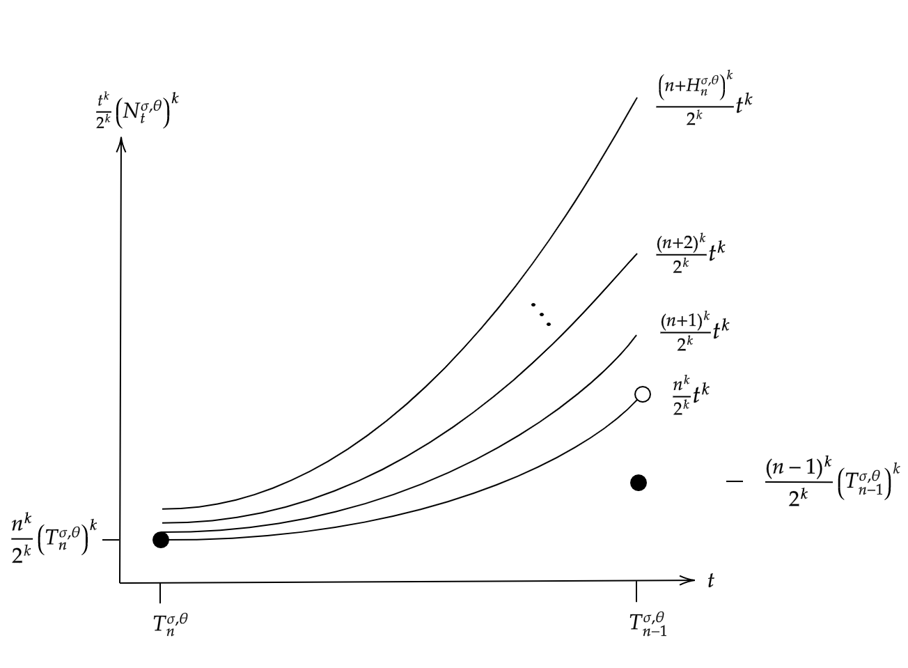
Figure 1: Possible trajectories of the function $(sN_{s}^{\sigma,\theta}/2)^{k}$ between the first hitting times of level $n$ and $n-1$.

Here the random variable $H_{n}^{\sigma,\theta}$ is defined as

$$H_{n}^{\sigma,\theta}:=\#\{s\in[T_{n}^{\sigma,\theta},T_{n-1}^{\sigma,\theta}):N_{s}^{\sigma,\theta}-N_{s-}^{\sigma,\theta}>0\}$$

or simply the number of times the ASG jumps up in this time window. From the diagram we see that the highest point that the process can reach is

$$\frac{\left(n+H_{n}^{\sigma,\theta}\right)^{k}}{2^{k}}\left(T_{n-1}^{\sigma,\theta}\right)^{k}=\sum_{j=0}^{k}\binom{k}{j}\frac{n^{k-j}}{2^{k}}\left(H_{n}^{\sigma,\theta}\right)^{j}\left(T_{n-1}^{\sigma,\theta}\right)^{k}.$$ (28)

We can now proceed by looking at the supremum of the above random variables over all $n$ since

$$\sup_{s\leq t}\left(\frac{sN_{s}^{\sigma,\theta}}{2}\right)^{k}\leq\sup_{n\in\mathbb{N}}\frac{\left(n+H_{n}^{\sigma,\theta}\right)^{k}}{2^{k}}\left(T_{n-1}^{\sigma,\theta}\right)^{k},$$ (29)

for any $t\geq 0$. Before stating our result however, we need to know more about the moments of $H_{n}^{\sigma,\theta}$. In the proof of [5, Lemma 4.1] it is shown, for a general birth/death process $N_{t}$ with birth/death rates $\lambda_{n}$ and $\mu_{n}$, that if (9) holds then the associated $H_{n}$ random variable

$$H_{n}:=\#\{s\in[T_{n},T_{n-1}):N_{s}-N_{s-}>0\}$$

satisfies

$$\mathbb{E}_{\infty}\left[H_{n}^{2}\right]\leq C\frac{\lambda_{n}}{\mu_{n}},$$

for some constant $C\geq 0$, for all $n\in\mathbb{N}$. Since we need to consider higher moments of $H_{n}^{\sigma,\theta}$, this inequality is not enough. As such, we extend the above inequality to all moments of $H_{n}$ for general birth/death processes:

Lemma 4.4.

Let $(N_{t})_{t\geq 0}$ be a birth/death process with birth/death rates $\lambda_{n}$ and $\mu_{n}$ respectively. If (9) holds then for each $k\in\mathbb{N}$ there exists $c_{k}>0$ such that

$$\mathbb{E}_{\infty}\left[H_{n}^{k}\right]\leq c_{k}\frac{\lambda_{n}}{\mu_{n}},~{}~{}n\geq 1.$$ (30)

Proof.

We follow a similar method of proof as in [5, Lemma 4.1] by first noting the random variable $H_{n}$ is simply the number of positive jumps before $T_{n-1}$ of a discrete-time random walk started at $n$ with transition probabilities $p_{i,i+1}=\lambda_{i}/(\lambda_{i}+\mu_{i})$ and $p_{i,i-1}=\mu_{i}/(\lambda_{i}+\mu_{i})$.

Next, we note that Lemma 3.1 also holds in the discrete-time case and so since (9) holds we have that $H_{n}$, for $n\geq n_{0}$, is stochastically dominated by $T$, the hitting time of $n-1$ by a discrete-time simple random walk started at $n$ with up/down transition probabilities $p$, $1-p$ respectively; note that this is the same $p$ from (11). Since $p<1/2$, all moments of $T$—and thus $H_{n}$ for $n\geq n_{0}$—are finite. Finiteness of moments of $H_{n}$ for $n<n_{0}$ can be obtained through the following recursive relationship:

$$\mathbb{E}_{\infty}[H_{n}]=\frac{\lambda_{n}}{\lambda_{n}+\mu_{n}}(1+\mathbb{E}_{\infty}[H_{n+1}]+\mathbb{E}_{\infty}[H_{n}]).$$

We now consider the Laplace transform of $H_{n}$, denoted $\hat{G}_{n}(a):=\mathbb{E}_{\infty}\left[\text{exp}(-aH_{n})\right]$, and the recursion formula (4.3) from [5]:

$$\hat{G}_{n}(a)=\frac{\mu_{n}}{\lambda_{n}+\mu_{n}}+\frac{\lambda_{n}}{\lambda_{n}+\mu_{n}}\text{exp}(-a)\hat{G}_{n}(a)\hat{G}_{n+1}(a),\qquad a\geq 0,\,n\geq 1.$$

Differentiating $k$ times gives us

$$\hat{G}_{n}^{(k)}(a)=\frac{\lambda_{n}}{\lambda_{n}+\mu_{n}}\sum_{\begin{subarray}{c}|\bm{m}|=k\\ \bm{m}\in\mathbb{N}_{0}^{3}\end{subarray}}\binom{k}{\bm{m}}(-1)^{m_{1}}\text{exp}(-a)\hat{G}_{n}^{(m_{2})}(a)\hat{G}_{n+1}^{(m_{3})}(a),$$

where $\mathbb{N}_{0}=\mathbb{N}\cup\{0\}$. If we now evaluate the above at $a=0$ we get

$$\mathbb{E}_{\infty}\left[H_{n}^{k}\right]=\frac{\lambda_{n}}{\lambda_{n}+\mu_{n}}\sum_{\begin{subarray}{c}|\bm{m}|=k\\ \bm{m}\in\mathbb{N}_{0}^{3}\end{subarray}}\binom{k}{\bm{m}}\mathbb{E}_{\infty}\left[H_{n}^{m_{2}}\right]\mathbb{E}_{\infty}\left[H_{n+1}^{m_{3}}\right],$$

since a factor of $(-1)^{k}$ can be cancelled from both sides. Rearranging this we see that

$$\frac{\mu_{n}}{\lambda_{n}}\mathbb{E}_{\infty}\left[H_{n}^{k}\right]=\sum_{\begin{subarray}{c}|\bm{m}|=k\\ \bm{m}\neq(0,k,0)\end{subarray}}\binom{k}{\bm{m}}\mathbb{E}_{\infty}\left[H_{n}^{m_{2}}\right]\mathbb{E}_{\infty}\left[H_{n+1}^{m_{3}}\right].$$

Now, the right hand side of this equation is a finite combination of moments; each of which are bounded by the respective moment of $T$. Thus the right hand side can be bounded by some constant $c_{k}\geq 0$. This then gives us (30). ∎

With this we now know enough about the asymptotic behaviour of the random variables in (28) to state the following:

Proposition 4.5.

$$\lim_{t\to 0}\mathbb{E}\left[\sup_{s\leq t}\left(\frac{sN_{s}^{\sigma,\theta}}{2}-1\right)^{k}\right]=0,\qquad\forall k\in\mathbb{N}.$$ (31)

Proof.

The first thing to note is that as soon as the right hand side of (29) is bounded in expectation the result follows thanks to an application of (24) and the dominated convergence theorem in a similar way to the proof of Proposition 4.3.

We start by looking at the terms on the right hand side of (28) for $j\neq 0$. The aim here is to show that the expectations of these random variables are summable in $n$ and hence their supremum over $n$ has finite mean. Applying (30), (18), and the Cauchy-Schwarz inequality to these terms we obtain the following:

$$\mathbb{E}\left[\binom{k}{j}\frac{n^{k-j}}{2^{k}}\left(H_{n}^{\sigma,\theta}\right)^{j}\left(T_{n-1}^{\sigma,\theta}\right)^{k}\right] \leq\binom{k}{j}\frac{n^{k-j}}{2^{k}}\mathbb{E}\left[\left(H_{n}^{\sigma,\theta}\right)^{2j}\right]^{1/2}\mathbb{E}\left[\left(T_{n-1}^{\sigma,\theta}\right)^{2k}\right]^{1/2}$$

$$\leq\binom{k}{j}\frac{n^{k-j}}{2^{k}}\frac{c_{2j}^{1/2}}{n^{1/2}}\left(\frac{C_{2k}^{0,\theta}}{n^{2k}}+\frac{C_{2k}^{\sigma,\theta}}{n^{2k+1}}\right)^{1/2}$$

$$=O\left(n^{-j-1/2}\right).$$

This then gives us that the expectation of the terms on the right hand side of (28) are summable in $n$ as long as $j\neq 0$. Thus we have that their supremum over $n$ is finite in expectation.

Next we need to deal with the first term on the right hand side of (28); i.e. the term corresponding to $j=0$. Since

$$\sup_{n\in\mathbb{N}}\frac{n^{k}}{2^{k}}\left(T_{n-1}^{\sigma,\theta}\right)^{k}\leq\sup_{n\in\mathbb{N}}\left[\frac{n^{k}}{2^{k}}\left(T_{n-1}^{\sigma,\theta}\right)^{k}-\frac{n^{k}}{2^{k}}\left(T_{n-1}^{0,\theta}\right)^{k}\right]+\sup_{n\in\mathbb{N}}\frac{n^{k}}{2^{k}}\left(T_{n-1}^{0,\theta}\right)^{k}$$

it suffices to show that the right hand side of the above is finite in expectation. For the second term this follows immediately from (26) since $n^{k}(T_{n-1}^{0,\theta})^{k}/2^{k}$ are the right end points of the continuous pieces of the process $t^{k}(N_{t}^{0,\theta})^{k}/2^{k}$. For the first term we consider the increments in $n$ of these random variables and show they are absolutely summable. This gives the desired result since, for any real sequence $x_{n}$,

$$\sup_{n\in\mathbb{N}}x_{n}\leq x_{1}+\sum_{n\geq 1}|x_{n+1}-x_{n}|.$$

For us, the corresponding increment is

$$\left|\frac{(n+1)^{k}}{2^{k}}\left(T_{n}^{\sigma,\theta}\right)^{k}-\frac{(n+1)^{k}}{2^{k}}\left(T_{n}^{0,\theta}\right)^{k}-\frac{n^{k}}{2^{k}}\left(T_{n-1}^{\sigma,\theta}\right)^{k}+\frac{n^{k}}{2^{k}}\left(T_{n-1}^{0,\theta}\right)^{k}\right|$$

$$=\left|\left(\frac{(n+1)^{k}}{2^{k}}\left(T_{n}^{\sigma,\theta}\right)^{k}-\frac{n^{k}}{2^{k}}\left(T_{n-1}^{\sigma,\theta}\right)^{k}\right)-\left(\frac{(n+1)^{k}}{2^{k}}\left(T_{n}^{0,\theta}\right)^{k}-\frac{n^{k}}{2^{k}}\left(T_{n-1}^{0,\theta}\right)^{k}\right)\right|.$$ (32)

Now, the terms inside the brackets are just the difference between successive right endpoints of continuous pieces of the processes $\left(sN_{s}^{\sigma,\theta}/2\right)^{k}$ and $\left(sN_{s}^{0,\theta}/2\right)^{k}$ respectively. These can be expressed in the following way:

$$\frac{(n+1)^{k}}{2^{k}}\left(T^{\sigma,\theta}_{n}\right)^{k}-\frac{n^{k}}{2^{k}}\left(T^{\sigma,\theta}_{n-1}\right)^{k}$$

$$=\left[(n+1)^{k}-n^{k}\right]\frac{\left(T^{\sigma,\theta}_{n}\right)^{k}}{2^{k}}-\frac{n^{k}}{2^{k}}\left(\left(T^{\sigma,\theta}_{n-1}\right)^{k}-\left(T^{\sigma,\theta}_{n}\right)^{k}\right)$$

$$=\frac{\left(T^{\sigma,\theta}_{n}\right)^{k}}{2^{k}}\left(\sum_{j=1}^{k}\binom{k}{j}\frac{n^{k-j}}{2^{k}}\right)-\frac{n^{k}}{2^{k}}\left(\sum_{j=1}^{k}\binom{k}{j}\left(T^{\sigma,\theta}_{n}\right)^{k-j}\left(T^{\sigma,\theta}_{n,n-1}\right)^{j}\right),$$ (33)

since $(T^{\sigma,\theta}_{n-1})^{k}=(T^{\sigma,\theta}_{n}+T^{\sigma,\theta}_{n,n-1})^{k}$. Note that one can set $\sigma=0$ in the above meaning these equalities apply to both the Kingman coalescent and the ASG. Using the substitution (33), (32) is then equal to

$$\left|\sum_{j=1}^{k}\binom{k}{j}\frac{n^{k-j}}{2^{k}}\left[\left(T_{n}^{\sigma,\theta}\right)^{k}-\left(T_{n}^{0,\theta}\right)^{k}\right]\right.$$

$${}-\frac{n^{k}}{2^{k}}\left.\sum_{j=1}^{k}\binom{k}{j}\left(\left(T_{n}^{\sigma,\theta}\right)^{k-j}\left(T_{n,n-1}^{\sigma,\theta}\right)^{j}-\left(T_{n}^{0,\theta}\right)^{k-j}\left(T_{n,n-1}^{0,\theta}\right)^{j}\right)\right|$$

$$\leq{} \sum_{j=1}^{k}\binom{k}{j}\frac{n^{k-j}}{2^{k}}\left|\left(T_{n}^{\sigma,\theta}\right)^{k}-\left(T_{n}^{0,\theta}\right)^{k}\right|$$ (34)

$${}+\frac{n^{k}}{2^{k}}\sum_{j=1}^{k}\binom{k}{j}\left|\left(T_{n}^{\sigma,\theta}\right)^{k-j}\left(T_{n,n-1}^{\sigma,\theta}\right)^{j}-\left(T_{n}^{0,\theta}\right)^{k-j}\left(T_{n,n-1}^{0,\theta}\right)^{j}\right|.$$

If we now apply expectations to (34), then the expectation of (32) is bounded by

$$\mathbb{E} \left[\Big{|}\frac{(n+1)^{k}}{2^{k}}\left(T_{n}^{\sigma,\theta}\right)^{k}-\frac{(n+1)^{k}}{2^{k}}\left(T_{n}^{0,\theta}\right)^{k}-\frac{n^{k}}{2^{k}}\left(T_{n-1}^{\sigma,\theta}\right)^{k}+\frac{n^{k}}{2^{k}}\left(T_{n-1}^{0,\theta}\right)^{k}\Big{|}\right]$$

$$\leq{} \sum_{j=1}^{k}\binom{k}{j}\frac{n^{k-j}}{2^{k}}\mathbb{E}\left[\Big{|}\left(T_{n}^{\sigma,\theta}\right)^{k}-\left(T_{n}^{0,\theta}\right)^{k}\Big{|}\right]$$

$${}+\frac{n^{k}}{2^{k}}\sum_{j=1}^{k}\binom{k}{j}\mathbb{E}\left[\Big{|}\left(T_{n}^{\sigma,\theta}\right)^{k-j}\left(T_{n,n-1}^{\sigma,\theta}\right)^{j}-\left(T_{n}^{0,\theta}\right)^{k-j}\left(T_{n,n-1}^{0,\theta}\right)^{j}\Big{|}\right]$$

$$\leq{} \sum_{j=1}^{k}\binom{k}{j}\frac{n^{k-j}}{2^{k}}\mathbb{E}\left[\Big{|}\left(T_{n}^{\sigma,\theta}\right)^{k}-\left(T_{n}^{0,\theta}\right)^{k}\Big{|}\right]$$

$${}+\frac{n^{k}}{2^{k}}\sum_{j=1}^{k}\binom{k}{j}\mathbb{E}\left[\left(T_{n}^{\sigma,\theta}\right)^{k-j}\Big{|}\left(T_{n,n-1}^{\sigma,\theta}\right)^{j}-\left(T_{n,n-1}^{0,\theta}\right)^{j}\Big{|}\right]$$

$${}+\frac{n^{k}}{2^{k}}\sum_{j=1}^{k}\binom{k}{j}\mathbb{E}\left[\left(T_{n,n-1}^{0,\theta}\right)^{j}\Big{|}\left(T_{n}^{\sigma,\theta}\right)^{k-j}-\left(T_{n}^{0,\theta}\right)^{k-j}\Big{|}\right].$$

Recalling equations (6) and (7) from Section 2, we see that on the joint probability space we have constructed the hitting times for the ASG are almost surely longer than the corresponding hitting times for the Kingman coalescent with mutation. This allows us to drop modulus signs from inside the above expectations. Combining this with (18), (13), and (17) results in the following inequality:

$$\mathbb{E}\left[\Big{|}\frac{(n+1)^{k}}{2^{k}}\left(T_{n}^{\sigma,\theta}\right)^{k}-\frac{(n+1)^{k}}{2^{k}}\left(T_{n}^{0,\theta}\right)^{k}-\frac{n^{k}}{2^{k}}\left(T_{n-1}^{\sigma,\theta}\right)^{k}+\frac{n^{k}}{2^{k}}\left(T_{n-1}^{0,\theta}\right)^{k}\Big{|}\right]$$

$$\leq{} \sum_{j=1}^{k}\binom{k}{j}\frac{n^{k-j}}{2^{k}}\frac{C_{k}^{\sigma,\theta}}{n^{k+1}}$$

$${}+\frac{n^{k}}{2^{k}}\sum_{j=1}^{k}\binom{k}{j}\left[\left(\frac{C_{k-j}^{0,\theta}}{n^{k-j}}+\frac{C_{k-j}^{\sigma,\theta}}{n^{k-j+1}}\right)\frac{B_{j}^{\sigma,\theta}}{n^{2j+1}}+\frac{2^{j}}{n^{j}(n-1+\theta)^{j}}\frac{C_{j}^{\sigma,\theta}}{n^{k-j+1}}\right]$$

$$={} O(n^{-2}).$$

From this we can conclude that the right hand side of (29) is finite in expectation and so the result follows. ∎

5 Proof of Theorem 1.1

In order to prove Theorem 1.1 we extend the arguments of Limic and Talarczyk [6] with modifications where needed. Lemmas 5.2 and 5.3 are analogues of Lemmas 2.2 and 2.3 from [6] for the ASG. Though the methods of proof are similar, they rely heavily on our PRM construction of the ASG and the results from Section 4; most importantly Proposition 4.5. Regardless of the similarities we present the results here in full in order to keep the proof self-contained.

Before establishing the key lemmas needed to prove Theorem 1.1 we state a technical lemma from [11] that is used repeatedly in what follows.

Lemma 5.1 ([11, Lemma 10]).

Suppose $f,g:[a,b]\rightarrow\mathbb{R}$ are càdlàg functions such that

$$\sup_{x\in[a,b]}\limits\left|f(x)+\int_{a}^{x}g(u)\,{{\rm{d}}}u\right|\leq K,$$

for some $K<\infty$. If, in addition $f(x)g(x)>0,~{}x\in[a,b]$, whenever $f(x)\neq 0$, then

$$\sup_{x\in[a,b]}\left|\int_{a}^{x}g(u)\,{{\rm{d}}}u\right|\leq K\text{ and}\sup_{x\in[a,b]}\left|f(x)\right|\leq 2K.$$ (35)

The first lemma we establish gives a formula for $tN_{t}^{\sigma,\theta}/2$ which helps us in analysing its small time behaviour.

Lemma 5.2.

Under the assumptions of Theorem 1.1 we have

$$\frac{tN_{t}^{\sigma,\theta}}{2}=1-\int_{0}^{t}\left(\frac{sN_{s}^{\sigma,\theta}}{2}-1\right)\frac{1}{s}\,{{\rm{d}}}s-M^{\sigma,\theta}_{t}+R^{\sigma,\theta}_{t},~{}~{}~{}t\geq 0,$$ (36)

where

$$M^{\sigma,\theta}_{t}=\frac{1}{2}\int_{0}^{t}\int_{\bar{\Delta}}s\mathbbm{1}_{\bar{\Delta}_{N_{s-}^{\sigma,\theta}}}(\bm{k})\left[\mathbbm{1}_{j>0}(\bm{k})-\mathbbm{1}_{j=0}(\bm{k})\right]\hat{\pi}({{\rm{d}}}s,{\rm{d}}\bm{k}),~{}~{}~{}t\geq 0,$$ (37)

and $R^{\sigma,\theta}$ is a continuous process such that for any $T>0$ there exists $C_{1}>0$ such that

$$\mathbb{E}\left[\sup_{s\leq t}|R^{\sigma,\theta}_{s}|\right]\leq C_{1}t,~{}~{}~{}t\leq T.$$ (38)

Proof.

Letting $0<r\leq t$, the PRM construction in Section 2 allows us to write the process as follows

$$N_{t}^{\sigma,\theta}={} N_{r}^{\sigma,\theta}-\int_{(r,t]}\int_{\bar{\Delta}}\mathbbm{1}_{\bar{\Delta}_{N_{s-}^{\sigma,\theta}}}(\bm{k})\left[\mathbbm{1}_{j>0}(\bm{k})-\mathbbm{1}_{j=0}(\bm{k})\right]\pi({{\rm{d}}}s,{\rm{d}}\bm{k}),$$

$$={} N_{r}^{\sigma,\theta}-\int_{(r,t]}\int_{\bar{\Delta}}\mathbbm{1}_{\bar{\Delta}_{N_{s-}^{\sigma,\theta}}}(\bm{k})\left[\mathbbm{1}_{j>0}(\bm{k})-\mathbbm{1}_{j=0}(\bm{k})\right]\nu({\rm{d}}s,{\rm{d}}\bm{k})$$

$${}-\int_{(r,t]}\int_{\bar{\Delta}}\mathbbm{1}_{\bar{\Delta}_{N_{s-}^{\sigma,\theta}}}(\bm{k})\left[\mathbbm{1}_{j>0}(\bm{k})-\mathbbm{1}_{j=0}(\bm{k})\right]\hat{\pi}({\rm{d}}s,{\rm{d}}\bm{k}),$$

$$={} N_{r}^{\sigma,\theta}-\int_{(r,t]}\frac{N_{s}^{\sigma,\theta}(N_{s}^{\sigma,\theta}-1+\theta-\sigma)}{2}\,{\rm{d}}s$$

$${}-\int_{(r,t]}\int_{\bar{\Delta}}\mathbbm{1}_{\bar{\Delta}_{N_{s-}^{\sigma,\theta}}}(\bm{k})\left[\mathbbm{1}_{j>0}(\bm{k})-\mathbbm{1}_{j=0}(\bm{k})\right]\hat{\pi}({\rm{d}}s,{\rm{d}}\bm{k}).$$

Since all jump times are isolated and countable then this representation is permissible. From integration by parts we also get that

$$tN_{t}^{\sigma,\theta}=rN_{r}^{\sigma,\theta}+\int_{(r,t]}N_{s}^{\sigma,\theta}\,{\rm{d}}s+\int_{(r,t]}s\,{\rm{d}}N_{s}^{\sigma,\theta}.$$

Combining these we obtain

$$\frac{tN_{t}^{\sigma,\theta}}{2}= \frac{rN_{r}^{\sigma,\theta}}{2}+\int_{(r,t]}\left(\frac{N_{s}^{\sigma,\theta}}{2}-s\frac{N_{s}^{\sigma,\theta}(N_{s}^{\sigma,\theta}-1+\theta-\sigma)}{4}\right)\,{\rm{d}}s$$

$$\hskip 56.9055pt-\int_{(r,t]}\int_{\bar{\Delta}}\frac{s}{2}\mathbbm{1}_{\bar{\Delta}_{N_{s-}^{\sigma,\theta}}}(\bm{k})\left[\mathbbm{1}_{j>0}(\bm{k})-\mathbbm{1}_{j=0}(\bm{k})\right]\hat{\pi}({\rm{d}}s,{\rm{d}}\bm{k}).$$ (39)

Next we need to check that one can formally let $r=0$ in the above expression, recognise that the final term is then equal to $M^{\sigma,\theta}_{t}$, and rearrange the drift term to reflect the formula in (36).

Starting with the final term in (39), we first need to fix $T\geq 0$ and use (31) to find that, for $t\leq T$

$$\mathbb{E}\left[\sup_{s\leq t}\left(\frac{sN_{s}^{\sigma,\theta}}{2}\right)^{k}\right]<\infty.$$ (40)

We can then use properties of the compensated Poisson integral to bound the second moment of the martingale (37):

$$\mathbb{E}[(M^{\sigma,\theta}_{t})^{2}] =\mathbb{E}\left[\int_{0}^{t}\int_{\bar{\Delta}}\frac{s^{2}}{4}\mathbbm{1}_{\bar{\Delta}_{N^{\sigma,\theta}_{s-}}}(\bm{k})\nu({\rm{d}}s,{\rm{d}}\bm{k})\right]$$

$$=\mathbb{E}\left[\int_{0}^{t}s^{2}\frac{N_{s}^{\sigma,\theta}(N_{s}^{\sigma,\theta}-1+\theta+\sigma)}{8}\,{\rm{d}}s\right]$$

$$\leq\mathbb{E}\left[\int_{0}^{t}s^{2}\frac{(N_{s}^{\sigma,\theta})^{2}}{8}+Ts\frac{(\theta+\sigma)N_{s}^{\sigma,\theta}}{8}\,{\rm{d}}s\right]$$ (41)

$$\leq C_{2}t,\qquad t\leq T,$$ (42)

where $C_{2}\geq 0$ comes from (40) with $k=1,2$.

It should be noted that the constant above (and most of the constants that follow) have an implicit dependence on $T$; though since we are concerned with behaviour near zero this dependence is unimportant. Thanks to [12, Theorem 8.23] and (42) we get that $M^{\sigma,\theta}$ given by (37) is a well defined square integrable martingale. Moreover, Doob’s $L^{2}$ maximal inequality gives us the following bound:

$$\mathbb{E}\left[\sup_{s\leq t}(M^{\sigma,\theta}_{s})^{2}\right]\leq 4C_{2}t,\qquad\forall t\leq T.$$ (43)

We note that the final term in (39) is equal to $M^{\sigma,\theta}_{t}-M^{\sigma,\theta}_{r}$ and by (43) we have $M^{\sigma,\theta}_{r}\to 0$ in $L^{2}$ as $r\to 0$.

Next, we rewrite the integral with respect to $s$ in (39) as

$$A^{\sigma,\theta}_{r}(t) :=\frac{1}{2}\int_{(r,t]}N^{\sigma,\theta}_{s}\,{\rm{d}}s-\frac{1}{2}\int_{(r,t]}s\frac{N_{s}^{\sigma,\theta}(N_{s}^{\sigma,\theta}-1+\theta-\sigma)}{2}\,{\rm{d}}s$$

$$\phantom{:}=-\int_{(r,t]}\frac{N_{s}^{\sigma,\theta}}{2}\left(\frac{s}{2}N_{s}^{\sigma,\theta}-1\right)\,{\rm{d}}s+\int_{(r,t]}\frac{s(1-\theta+\sigma)}{4}N_{s}^{\sigma,\theta}\,{\rm{d}}s.$$ (44)

This allows us to rearrange (39) into the following:

$$\frac{t}{2}N_{t}^{\sigma,\theta}-1+\int_{(r,t]}\frac{N_{s}^{\sigma,\theta}}{2}\left(\frac{s}{2}N_{s}^{\sigma,\theta}-1\right)\,{\rm{d}}s={} \frac{r}{2}N_{r}^{\sigma,\theta}-1+\int_{(r,t]}\frac{(1-\theta+\sigma)s}{4}N_{s}^{\sigma,\theta}\,{\rm{d}}s$$

$${}-(M^{\sigma,\theta}_{t}-M^{\sigma,\theta}_{r}).$$

Applying (35) with $f(s)=sN_{s}^{\sigma,\theta}/2-1$, $g(s)=N_{s}^{\sigma,\theta}(sN_{s}^{\sigma,\theta}/2-1)/2$, $a=r$, and $b=t$ we find that

$$\sup_{r\leq s\leq t}\left|\frac{s}{2}N_{s}^{\sigma,\theta}-1\right|\leq{} 2\Bigg{(}\left|\frac{r}{2}N_{r}^{\sigma,\theta}-1\right|+|M^{\sigma,\theta}_{r}|$$

$$+\sup_{r\leq s\leq t}|M^{\sigma,\theta}_{s}|+\int_{(r,t]}\left|\frac{(1-\theta+\sigma)s}{4}N_{s}^{\theta}\right|\,{\rm{d}}s\Bigg{)}.$$

Letting $r\to 0$ in the above and using (24) gives us

$$\sup_{s\leq t}\left|\frac{s}{2}N_{s}^{\sigma,\theta}-1\right|\leq 2\left(\sup_{s\leq t}|M^{\sigma,\theta}_{s}|+\int_{0}^{t}\left|\frac{(1-\theta+\sigma)s}{4}N_{s}^{\sigma,\theta}\right|\,{\rm{d}}s\right),$$ (45)

where letting $r=0$ in the integral on the right hand side is permissible thanks to (40) with $k=1$. Squaring both sides of (45), applying expectations and using (43) and (40) gives us that there exists $C_{3}>0$ such that

$$\mathbb{E}\left[\sup_{s\leq t}\left(\frac{sN_{s}^{\sigma,\theta}}{2}-1\right)^{2}\right]\leq C_{3}t,\qquad\forall t\leq T.$$ (46)

We can now use this bound, which improves on (31), to ensure the integral term in (36) is well-defined. Letting $X^{\sigma,\theta}_{t}:=X_{1}^{\sigma,\theta}(t)=tN_{t}^{\sigma,\theta}/2-1$, (46) (along with Jensen’s inequality) allows us to control $X_{t}^{\sigma,\theta}$ as follows:

$$-\sqrt{C_{3}t}\leq\mathbb{E}\left[X_{t}^{\sigma,\theta}\right]\leq\sqrt{C_{3}t},$$ (47)

for $t\leq T$. If we now consider the integral term in (36) we see that by (47)

$$\mathbb{E}\left[\int_{0}^{t}X^{\sigma,\theta}_{s}\frac{1}{s}\,{\rm{d}}s\right]=\int_{0}^{t}\mathbb{E}\left[X^{\sigma,\theta}_{s}\right]\frac{1}{s}\,{\rm{d}}s\leq\int_{0}^{t}\frac{\sqrt{C_{3}}}{\sqrt{s}}\,{\rm{d}}s=2\sqrt{C_{3}t}.$$

This shows that the integral with respect to $s$ in (36) has finite expectation and thus is finite a.s. and so is well-defined.

Next, we can express $A^{\sigma,\theta}_{r}(t)$ as

$$A^{\sigma,\theta}_{r}(t)={} -\int_{(r,t]}\left(\frac{s}{2}N_{s}^{\sigma,\theta}-1\right)^{2}\frac{1}{s}\,{\rm{d}}s-\int_{(r,t]}\left(\frac{s}{2}N_{s}^{\sigma,\theta}-1\right)\frac{1}{s}\,{\rm{d}}s$$

$${}+\frac{1}{2}\int_{(r,t]}\frac{(1-\theta+\sigma)s}{2}N_{s}^{\sigma,\theta}\,{\rm{d}}s.$$

Using (46) along with (40) we find that

$$\mathbb{E}\left[\Big{|}A^{\sigma,\theta}_{r}(t)+\int_{(r,t]}\left(\frac{s}{2}N_{s}^{\sigma,\theta}-1\right)\frac{1}{s}\,{\rm{d}}s\Big{|}\right]\leq C_{4}t,\qquad\forall t\leq T,$$

where $C_{4}>0$ does not depend on $r$. This shows that, as $r\to 0$, $A^{\sigma,\theta}_{r}(t)$ converges in $L^{1}$ to

$$-\int_{0}^{t}\left(\frac{sN_{s}^{\sigma,\theta}}{2}-1\right)\frac{1}{s}\,{\rm{d}}s+R^{\sigma,\theta}_{t},$$

where

$$R^{\sigma,\theta}_{t}:=-\int_{0}^{t}\left(\frac{s}{2}N_{s}^{\sigma,\theta}-1\right)^{2}\frac{1}{s}\,{\rm{d}}s+\frac{1}{2}\int_{0}^{t}\frac{(1-\theta+\sigma)s}{2}N_{s}^{\sigma,\theta}\,{\rm{d}}s.$$ (48)

To conclude, (46) applied to the first term on the right hand side of (48) and (40) applied to the second term yield the bound in (38). ∎

Next, we will reduce the problem of convergence of (5) to convergence of the following process defined via the martingale (37):

$$Y_{t}^{\sigma,\theta} :=-\frac{1}{t}\int_{0}^{t}u\,{\rm{d}}M_{u}^{\sigma,\theta},~{}~{}t>0,~{}~{}Y_{0}^{\sigma,\theta}=0,$$ (49)

$$Y_{\varepsilon}^{\sigma,\theta}(t) :=\varepsilon^{-1/2}Y_{\varepsilon t}^{\sigma,\theta}.$$ (50)

Lemma 5.3.

The process $(Y_{t}^{\sigma,\theta})_{t\geq 0}$ satisfies the equation

$$Y_{t}^{\sigma,\theta}=-\int_{0}^{t}Y_{s}^{\sigma,\theta}\frac{1}{s}\,{\rm{d}}s-M_{t}^{\sigma,\theta}.$$ (51)

Moreover, there exists $C_{5}>0$ such that for any $t\leq T$

$$\mathbb{E}\left[\sup_{s\leq t}\left(Y_{s}^{\sigma,\theta}\right)^{2}\right]\leq C_{5}t.$$ (52)

Finally, we have that

$$\lim_{\varepsilon\to 0}\mathbb{E}\left[\sup_{s\leq t}\left|X_{\varepsilon}^{\sigma,\theta}(s)-Y_{\varepsilon}^{\sigma,\theta}(s)\right|\right]=0.$$ (53)

Proof.

First we consider $L^{\sigma,\theta}_{t}:=tY^{\sigma,\theta}_{t}$ so that $L^{\sigma,\theta}$ is a square integrable martingale with quadratic variation

$$\left[L^{\sigma,\theta}\right]_{t}=\frac{1}{4}\int_{0}^{t}\int_{\bar{\Delta}}s^{4}\mathbbm{1}_{\bar{\Delta}_{N_{s-}^{\sigma,\theta}}}(\bm{k})\pi({\rm{d}}s,{\rm{d}}\bm{k}),$$

which has expectation

$$\mathbb{E}\left[[L^{\sigma,\theta}]_{t}\right] =\frac{1}{4}\mathbb{E}\left[\int_{0}^{t}\int_{\bar{\Delta}}s^{4}\mathbbm{1}_{\bar{\Delta}_{N_{s-}^{\sigma,\theta}}}(\bm{k})\nu({\rm{d}}s,{\rm{d}}\bm{k})\right]$$

$$=\frac{1}{4}\mathbb{E}\left[\int_{0}^{t}s^{2}\left(s^{2}\frac{N_{s}^{\sigma,\theta}(N_{s}^{\sigma,\theta}-1+\theta+\sigma)}{2}\right)\,{\rm{d}}s\right]$$ (54)

$$\leq C_{2}\int_{0}^{t}s^{2}\,{\rm{d}}s=\frac{C_{2}}{3}t^{3},$$ (55)

where we use the same bound from (42) on the expectation of the bracketed term in (54).

This now gives us that

$$\mathbb{E}\left[\left(Y^{\sigma,\theta}_{t}\right)^{2}\right]=\frac{1}{t^{2}}\mathbb{E}\left[\left(L^{\sigma,\theta}_{t}\right)^{2}\right]=\frac{1}{t^{2}}\mathbb{E}\left[[L^{\sigma,\theta}]_{t}\right]\leq\frac{C_{2}}{3}t.$$ (56)

In order to obtain (51) we first use integration by parts to write

$$Y^{\sigma,\theta}_{t}-Y^{\sigma,\theta}_{r} =\int_{(r,t]}\frac{1}{s^{2}}\int_{0}^{s}u\,{\rm{d}}M^{\sigma,\theta}_{u}\,{\rm{d}}s-\int_{(r,t]}\,{\rm{d}}M^{\sigma,\theta}_{s}$$

$$=-\int_{(r,t]}\frac{1}{s}Y^{\sigma,\theta}_{s}\,{\rm{d}}s-M^{\sigma,\theta}_{t}+M^{\sigma,\theta}_{r},$$ (57)

and let $r\to 0$; using (56) and Jensen’s inequality to bound $\mathbb{E}[\int_{(r,t]}|Y^{\sigma,\theta}_{s}|/s\,{\rm{d}}s]$ uniformly in $r>0$ by $2\sqrt{Ct}/\sqrt{3}$, ensuring that $\int_{0}^{t}Y^{\sigma,\theta}_{s}/s\,{\rm{d}}s$ exists almost surely.

Now, we apply (35) with $f(s):=Y^{\sigma,\theta}_{s}$, $g(s):=Y^{\sigma,\theta}_{s}/s$, $a=0$ and $b=t$ to get that

$$\sup_{s\leq t}|Y^{\sigma,\theta}_{s}|\leq 2\sup_{s\leq t}M^{\sigma,\theta}_{s}.$$

We can then square both sides and apply expectations along with (43) to obtain (52).

To prove (53) we first recall that $X^{\sigma,\theta}_{t}=tN_{t}^{\theta}/2-1$ and so by Lemma 5.2 and (51),

$$X^{\sigma,\theta}_{t}-Y^{\sigma,\theta}_{t}=-\int_{0}^{t}(X^{\sigma,\theta}_{s}-Y^{\sigma,\theta}_{s})\frac{1}{s}\,{\rm{d}}s+R^{\theta}_{t}.$$ (58)

Applying (35) to the above we find that

$$\sup_{s\leq t}|X^{\sigma,\theta}_{s}-Y^{\sigma,\theta}_{s}|\leq 2\sup_{s\leq t}|R^{\sigma,\theta}_{s}|.$$

This leads to

$$\mathbb{E}\left[\sup_{s\leq t}\left|X^{\sigma,\theta}_{\varepsilon}(s)-Y^{\sigma,\theta}_{\varepsilon}(s)\right|\right] =\varepsilon^{-1/2}\mathbb{E}\left[\sup_{s\leq t}\left|X^{\sigma,\theta}(\varepsilon s)-Y^{\sigma,\theta}(\varepsilon s)\right|\right]$$

$$\leq 2\varepsilon^{-1/2}\mathbb{E}\left[\sup_{s\leq t}|R^{\sigma,\theta}_{\varepsilon s}|\right]$$

$$\leq 2C_{1}\sqrt{\varepsilon}t,$$

using (38). Letting $\varepsilon\to 0$ in the above gives us (53). ∎

We now have everything in place to prove Theorem 1.1. The proof consists of first checking the conditions of [13, Chapter 7, Theorem 1.4] are satisfied for the process

$$L^{\sigma,\theta}_{\varepsilon}(t):=-tY^{\sigma,\theta}_{\varepsilon}(t)=\frac{1}{\varepsilon^{3/2}}\int_{0}^{\varepsilon t}u\,{\rm{d}}M^{\sigma,\theta}_{u},\qquad t\geq 0,$$

and proving its convergence to $(tZ_{t})_{t\geq 0}$ as $\varepsilon\to 0$. Then, as in [6], we take advantage of Steps 2–4 in the proof of [14, Lemma 4.8] to extend this to the convergence of $Y_{\varepsilon}^{\sigma,\theta}$ to $Z$ as $\varepsilon\to 0$. Essentially, the continuity of $t\mapsto 1/t$ away from zero along with the control we have over these processes near zero is what ensures this convergence. Finally, (53) then gives us the convergence of (5) to (4).

Proof of Theorem 1.1.

Starting then with $L_{\varepsilon}^{\sigma,\theta}$, we first note that since $L^{\sigma,\theta}_{\varepsilon}(t)=-\varepsilon^{-3/2}L^{\sigma,\theta}(\varepsilon t)$, then $L^{\sigma,\theta}_{\varepsilon}$ is an $L^{2}$-martingale of the form

$$L^{\sigma,\theta}_{\varepsilon}(t)=\varepsilon^{-3/2}\frac{1}{2}\int_{0}^{\varepsilon t}\int_{\bar{\Delta}}s^{2}\mathbbm{1}_{\bar{\Delta}_{N_{s-}^{\sigma,\theta}}}(\bm{k})\left[\mathbbm{1}_{j>0}(\bm{k})-\mathbbm{1}_{j=0}(\bm{k})\right]\hat{\pi}({\rm{d}}s,{\rm{d}}\bm{k}).$$ (59)

The compensator of the square of this process is given by

$$\langle L^{\sigma,\theta}_{\varepsilon}\rangle_{t} =\frac{1}{4\varepsilon^{3}}\int_{0}^{\varepsilon t}\int_{\bar{\Delta}}s^{4}\mathbbm{1}_{\bar{\Delta}_{N_{s-}^{\sigma,\theta}}}(\bm{k})\nu({\rm{d}}s,{\rm{d}}\bm{k}),$$

$$=\frac{1}{4\varepsilon^{3}}\int_{0}^{\varepsilon t}s^{4}\frac{N_{s}^{\sigma,\theta}(N_{s}^{\sigma,\theta}-1+\theta+\sigma)}{2}\,{\rm{d}}s$$

$$=\frac{1}{2}\int_{0}^{t}s^{2}(\varepsilon s)^{2}\frac{N_{\varepsilon s}^{\sigma,\theta}(N_{\varepsilon s}^{\sigma,\theta}-1+\theta+\sigma)}{4}\,{\rm{d}}s.$$ (60)

We now wish to verify that the assumptions (b) in [13, Theorem 1.4, Chapter 7] are satisfied with $M_{n}$ corresponding to $L^{\sigma,\theta}_{\varepsilon}$, $A_{n}$ corresponding to $\langle L^{\sigma,\theta}_{\varepsilon}\rangle$ and $C_{t}=\int_{0}^{t}u^{2}\,{\rm{d}}u/2$.

First, we note that since $\langle L^{\sigma,\theta}_{\varepsilon}\rangle$ is continuous we only need to show (i) that $\langle L^{\sigma,\theta}_{\varepsilon}\rangle_{t}$ converges as $\varepsilon\to 0$ to $\int_{0}^{t}u^{2}/2\,{\rm{d}}u$ in probability for each $t>0$, and (ii) that for any $T>0$,

$$\lim_{\varepsilon\to 0}\mathbb{E}\left[\sup_{t\leq T}|L^{\sigma,\theta}_{\varepsilon}(t)-L^{\sigma,\theta}_{\varepsilon}(t-)|^{2}\right]=0.$$ (61)

For the first claim we consider the expected value of (60) as $\varepsilon\to 0$. Since the integrand is non-negative we can use Tonelli’s theorem to switch the order of integration:

$$\lim_{\varepsilon\to 0}\mathbb{E}\left[\frac{1}{2}\int_{0}^{t}s^{2}(\varepsilon s)^{2}\frac{N_{\varepsilon s}^{\sigma,\theta}(N_{\varepsilon s}^{\sigma,\theta}-1+\theta+\sigma)}{4}\,{\rm{d}}s\right]$$

$${}=\lim_{\varepsilon\to 0}\frac{1}{2}\int_{0}^{t}s^{2}\mathbb{E}\left[(\varepsilon s)^{2}\frac{N_{\varepsilon s}^{\sigma,\theta}(N_{\varepsilon s}^{\sigma,\theta}-1+\theta+\sigma)}{4}\right]\,{\rm{d}}s.$$

Similarly to (42), we can control $\mathbb{E}\left[(\varepsilon s)^{2}N_{\varepsilon s}^{\sigma,\theta}(N_{\varepsilon s}^{\sigma,\theta}-1+\theta+\sigma)/4\right]$ uniformly in $\varepsilon>0$, allowing us to bring the limit inside the integral. Expanding the brackets we now get

$$\frac{(\varepsilon s)^{2}(N_{\varepsilon s}^{\sigma,\theta})^{2}}{4}+\frac{(\sigma+\theta-1)(\varepsilon s)^{2}N_{\varepsilon s}^{\sigma,\theta}}{4}.$$

The first term converges to 1 and the second term goes to 0 both in $L^{1}$ thanks to (31). Thus (60) converges to $\int_{0}^{t}u^{2}\,{\rm{d}}u/2$ in probability as $\varepsilon\to 0$.

To address (ii): the limit in (61) holds since, thanks to the representation (59), the jumps of $L^{\sigma,\theta}_{\varepsilon}$ on $[0,T]$ are isolated and uniformly bounded by $\varepsilon^{-3/2}(\varepsilon T)^{2}/2$ which goes to zero as $\varepsilon\to 0$. Thus we have the convergence of $L^{\sigma,\theta}_{\varepsilon}\to(tZ_{t})_{t\geq 0}$ in law in $D_{\mathbb{R}}[0,\infty)$.

Before concluding the proof one needs the following bound on the limiting process $Z$:

$$\mathbb{E}\left[\sup_{s\leq t}Z_{s}^{2}\right]\leq C_{6}t,\qquad C_{6}\geq 0.$$

This bound follows from the formula

$$Z_{t}=-\int_{0}^{t}Z_{s}\frac{1}{s}\,{\rm{d}}s+\frac{1}{\sqrt{2}}W_{t},$$

in combination with (35), similarly to the proof of (52).

The rest of the proof uses Steps 2–4 of [14, Lemma 4.8] to show that convergence of $L^{\sigma,\theta}_{\varepsilon}$ implies the required convergence of $X_{\varepsilon}^{\sigma,\theta}$; see also the proof of Theorem 1.1 of [6]. ∎

References

- [1] J. Kingman, “The coalescent,” Stochastic Processes and their Applications, vol. 13, no. 3, pp. 235 – 248, 1982.
- [2] N. Berestycki, “Recent progress in coalescent theory,” Ensaios Matemáticos, vol. 16, pp. 1–193, 2009.
- [3] R. C. Griffiths, “Asymptotic line-of-descent distributions,” Journal of Mathematical Biology, vol. 21, pp. 67–75, 1984.
- [4] P. A. Jenkins and D. Spanò, “Exact simulation of the Wright–Fisher diffusion,” The Annals of Applied Probability, vol. 27, p. 1478–1509, Jun 2017.
- [5] V. Bansaye, S. Méléard, and M. Richard, “Speed of coming down from infinity for birth-and-death processes,” Advances in Applied Probability, vol. 48, no. 4, p. 1183–1210, 2016.
- [6] V. Limic and A. Talarczyk, “Diffusion limits at small times for -coalescents with a Kingman component,” Electron. J. Probab., vol. 20, p. 20 pp., 2015.
- [7] C. Neuhauser and S. M. Krone, “The genealogy of samples in models with selection,” Genetics, vol. 145, no. 2, pp. 519–534, 1997.
- [8] S. M. Krone and C. Neuhauser, “Ancestral processes with selection,” Theoretical Population Biology, vol. 51, no. 3, pp. 210 – 237, 1997.
- [9] R. Griffiths and P. Marjoram, “An ancestral recombination graph,” in Progress in population genetics and human evolution, pp. 257 – 270, Springer, 1997. Progress in population genetics and human evolution ; Conference date: 01-01-1997.
- [10] P. Donnelly and T. G. Kurtz, “Genealogical processes for fleming-viot models with selection and recombination,” Ann. Appl. Probab., vol. 9, pp. 1091–1148, 11 1999.
- [11] J. Berestycki, N. Berestycki, and V. Limic, “The -coalescent speed of coming down from infinity,” Ann. Probab., vol. 38, pp. 207–233, 01 2010.
- [12] S. Peszat and J. Zabczyk, Stochastic Partial Differential Equations with Lévy Noise: An Evolution Equation Approach. Encyclopedia of Mathematics and its Applications, Cambridge University Press, 2007.
- [13] S. N. Ethier and T. G. Kurtz, Markov processes – characterization and convergence. Wiley Series in Probability and Mathematical Statistics: Probability and Mathematical Statistics, New York: John Wiley & Sons Inc., 1986.
- [14] V. Limic and A. Talarczyk, “Second-order asymptotics for the block counting process in a class of regularly varying -coalescents,” Ann. Probab., vol. 43, pp. 1419–1455, 05 2015.