Combined subleading high-energy logarithms and NLO accuracy for W production in association with multiple jets

Abstract

Large logarithmic corrections in $\hat{s}/p_{t}^{2}$ lead to substantial variations in the perturbative predictions for inclusive $W$-plus-dijet processes at the Large Hadron Collider. This instability can be cured by summing the leading-logarithmic contributions in $\hat{s}/p_{t}^{2}$ to all orders in $\alpha_{s}$. As expected though, leading logarithmic accuracy is insufficient to guarantee a suitable description in regions of phase space away from the high energy limit.

We present (i) the first calculation of all partonic channels contributing at next-to-leading logarithmic order in $W$-boson production in association with at least two jets, and (ii) bin-by-bin matching to next-to-leading fixed-order accuracy. This new perturbative input is implemented in High Energy Jets, and systematically improves the description of available experimental data in regions of phase space which are formally subleading with respect to $\hat{s}/p_{t}^{2}$.

1 Introduction

The continuing success of the Large Hadron Collider (LHC) is challenging the theoretical particle physics community to continuously improve the precision of theory predictions. One challenge to our standard approaches is that the complexity of a perturbative scattering process increases for increasing centre-of-mass energy and fixed transverse scales. For example, LHC studies of additional jet activity from dijet systems in regions of phase space with large dijet invariant mass or rapidity separation Aad:2011jz ; Aad:2014pua reveal an amount of additional jet activity above and beyond what can be described by fixed-order NLO approaches. While predictions at NNLO exist for dijet production, such advanced predictions have not been applied to these analyses. Even at the 1.96 TeV Tevatron, analyses of additional jet activity in e.g. $W$-production in association with dijets at D0 Abazov:2013gpa consistently revealed a tension between data and the standard set of predictions in the same regions of phase space.

The issues identified with NLO predictions for very exclusive observables may not show up in the inclusive two-jet distributions in e.g. $m_{j_{1}j_{2}}$ or $\Delta y_{j_{1}j_{2}}$, but large variations and discrepancies are found, for example, in the description of additional QCD radiation in $W+$dijets and $Z+$dijets, see e.g. Aaboud:2017emo . Such studies are highly relevant in their own right, but are also necessary for the development of the systematic description of perturbative corrections to the QCD channel of Higgs boson+dijets production. This is particularly true within the phase space cuts used for the study of the Vector Boson Fusion channel. The similarity in the radiative corrections to the various processes is caused by the universality of the QCD radiation pattern arising from a colour octet exchange between jets.

The colour-octet exchange emphasises the contribution from real-emission, higher-order perturbative corrections and is also accompanied by a tower of logarithms from virtual corrections. Both sources of perturbative corrections are included in the BFKL equation Fadin:1975cb ; Kuraev:1976ge ; Kuraev:1977fs ; Balitsky:1978ic , which captures the dominant logarithms ($\ln\hat{s}/p_{t}^{2}$, where $\hat{s}$ is the partonic centre-of-mass energy and $p_{t}$ is the transverse momentum scale) that govern the high-energy limit of the on-shell scattering cross sections. Such logarithms are not systematically included in the standard perturbative methods for obtaining predictions for LHC observables.

The dominant logarithmic corrections to the $n$-jet production rate of the form $\alpha_{s}^{m}\ln^{m}\hat{s}/p_{t}^{2}$ (and, as introduced in this paper, specific subleading contributions of order $\alpha_{s}^{m+1}\ln^{m}\hat{s}/p_{t}^{2}$) are, however, systematically included in the calculations of the on-shell partonic scattering amplitudes within the framework of High Energy Jets (HEJ) Andersen:2009nu ; Andersen:2009he ; Andersen:2011hs ; Andersen:2012gk . The framework is based on a systematic power-expansion of the $n$-body on-shell scattering matrix element, which controls the logarithmic corrections from real emissions, coupled with the Lipatov Ansatz for the structure of the virtual corrections. The virtual corrections not only cancel the infrared poles from the real corrections, but also contribute to the finite part of the matrix element. This approach captures the logarithmic corrections from both real and virtual corrections, and indeed both are necessary for obtaining full logarithmic accuracy.

In HEJ, the sum over $n$ and the integration over each $n$-body phase space point is performed explicitly using Monte Carlo sampling, and as such the predictions are made at the partonic level with direct access to the 4-momenta of each of the $n$ particles. The framework merges fixed-order (currently leading order), high-multiplicity matrix elements with an all-order description of the dominant logarithms. The formalism has been implemented for several processes, and compares favourably to data in studies of the jet activity from dijet systems production Aad:2011jz ; Chatrchyan:2012gwa ; Aad:2014pua , also in association with electro-weak bosons Abazov:2013gpa ; Aad:2014qxa ; Aaboud:2017fye . These studies indicate that for large invariant mass, and large rapidity differences, the high-energy logarithms are important, and their systematic inclusion improves the accuracy of the theoretical prediction.

In this paper, for the first time, we apply the HEJ formalism to well-defined partonic channels in inclusive $W+$dijet production which are formally subleading in the high energy limit. This resummation of the LL corrections to partonic channels contributing at subleading level for $\alpha_{s}^{3}$ and $\alpha_{s}^{4}$ does not achieve full NLL accuracy for the rates of $W+$dijets, since it does not include the sub-leading corrections to the channels contributing also at LL level. However, the new contribution is well-defined, and as we will demonstrate, the inclusion of such subleading channels leads to a significantly improved description of transverse observables, and also to a lesser dependence of the predictions upon the matching to fixed-order.

In section 2, we commence by reviewing the scaling of the amplitude and the definition of leading and subleading channels in the high energy limit. We then define and explain the generic building blocks that are required for the amplitude-based approach used in the HEJ formalism. In section 3 we present the calculation of the new building blocks which are necessary for the inclusion of subleading channels. In section 4 we present a new method of matching which increases the fixed-order accuracy of our predictions for measured distributions to next-to-leading order. Finally we present comparisons of our results to experimental data in section 5 and our conclusions in section 6.

2 High Energy Scattering

2.1 Scaling of amplitudes and cross sections in the High Energy Limit

The all-order resummation in HEJ improves the perturbative description of scatterings by systematically including the dominant contributions from the logarithms in $\hat{s}/p_{t}^{2}$ which arise at each order in the coupling. The centre-of-mass energy of LHC collisions is such that these logarithms can become large and spoil the convergence of the perturbative series, particularly in analyses where a large rapidity separation or large invariant mass between jets is required. Within HEJ the calculation of the logarithmic contributions to the scattering amplitude is organised in terms of virtual and real corrections just like for standard fixed-order perturbation theory. The logarithmic expansion of the cross section relies on two concepts:

1. The kinematic regions important for the logarithmic accuracy,

2. The systematic approximation to the scattering amplitude, ensuring the logarithmic accuracy of the cross section in these regions.

2.1.1 Kinematic regions

Leading Logarithmic accuracy (LLA) in $\hat{s}/p_{t}^{2}$ is controlled by the Multi-Regge Kinematic (MRK) limit of the $2\to n$ scattering process, where the invariant mass between each set of particles is large, while all transverse scales are similar:

$$\forall i,j\in\{1,\ldots,n\},i\not=j:\quad s_{ij}\to\infty,\qquad|p_{i\perp}|\sim|p_{j\perp}|.$$ (1)

The set of $t$-momenta in the so-called non-overlapping channels, or planar diagrams (see fig. 1), are defined as

$$q_{i}=p_{a}-\sum_{l=1}^{i}p_{l}.$$ (2)

In the MRK limit

$$t_{i}=q_{i}^{2}\to-q_{i\perp}^{2}.$$ (3)

The reason that the logarithmic accuracy is controlled by the regions of MRK and Quasi Multi-Regge Kinematics (QMRK) will become clear after the discussion of the scaling of the amplitude in these limits.

Figure 1: An illustration of the definition of the $t$-channel momenta in non-overlapping channels or planar diagrams.

In fact, the MRK limit requires also the transverse part of these $t$-channel momenta to be finite in the MRK limit, such that the conditions in eq. (1) are supplemented with the requirement

$$\forall i,j:\ |q_{\perp i}|\sim|p_{\perp j}|$$ (4)

such that all transverse scales relevant for the evaluation of the amplitudes are similar.

If we let the indices increase with the ordering of the particles in rapidity, the MRK limit can also be expressed as

$$\begin{split}&\forall i\in\{1,\ldots,n-1\}:\ y_{i}\ll y_{i+1}\ \\ &\forall i\in\{1,\ldots,n-1\},j\in\{1,\ldots,n\}:|q_{\perp i}|\sim|p_{\perp j}|\sim p_{\perp},\end{split}$$ (5)

for some fixed $p_{\perp}$, and where the so-called strong ordering of rapidities means the limit of infinite rapidity separation between each neighbouring pair of particles. Next-to-Leading Logarithmic accuracy (NLLA) in $\hat{s}/p_{t}^{2}$ receives contributions also from all the $n-1$ QMRK limits, where the requirement of a large separation is relaxed for exactly one pair $(j,j+1)$ of particles with arbitrary $j\in\{1,\ldots,n-1\}$:

$$\forall i\in\{1,\ldots,n-1\},i\not=j:\quad y_{i}\ll y_{i+1},\qquad|q_{\perp i}|\sim p_{\perp}.$$ (6)

The factorising of scattering amplitudes in the QMRK will be further discussed in sections 2.1.2 and 2.2. With respect to the kinematic limits, in the QMRK the pair of momenta $(j,j+1)$ is treated as one momentum in the MRK considerations, and the limit requires just the size of the sum of transverse momenta $(j,j+1)$ to be small, and therefore the induced change in $|q_{i}|$ to be small.

2.1.2 Scaling of Scattering Amplitudes in the limits of MRK and QMRK

We will start this section with a discussion of the historical roots of the application of Regge theory in the study of the strong force. The scaling of amplitudes for the scattering of specific hadrons is described effectively using Regge theory for multi-particle production Brower:1974yv , describing the scaling with energy due to exchange of various specific mesons, e.g. $\pi^{0}$ or $\rho$. A partial wave expansion of the scattering amplitude exposes a connection between the spin of the exchanged particles and the scaling of the amplitude with energy. For the scattering $2\to n$ with momenta $ab\to 1\cdots n$, the scaling with $s$ in the MRK limit of the scattering amplitude is

$$\mathcal{M}\sim s_{12}^{\alpha_{1}(t_{1})}\ldots s_{n-1,n}^{\alpha_{n-1}(t_{n-1})}\gamma\,,$$ (7)

where the $s_{ij}$ are the invariant masses of rapidity-ordered pairs of particles. The $t_{i}$ are defined as $t_{i}=q_{i}^{2}$ with $q_{i}$ defined in eq. 2. The factor $\gamma$ depends on transverse scales only, which are suppressed compared to $s$ in the MRK and QMRK limits. The exponent of the invariant $s_{i,i+1}$, $\alpha_{i}(t_{i})$, is the effective spin of any possible particle exchanged in the $i^{\mathrm{th}}$ $t$-channel. The dominant contributions at large $s_{i,i+1}$ will therefore be generated from processes where the particles exchanged in the $t_{i}$-channel have the largest possible spin.

It is perhaps surprising that the partial wave analysis and the scaling of scattering amplitudes applies also to processes in the gauge theory of QCD. This insight was obtained in the seminal work Fadin:1975cb ; Kuraev:1976ge ; Kuraev:1977fs of Fadin, Kuraev and Lipatov. Naïvely, the quarks and gluons of QCD allow for a scaling of the amplitude itself with invariants of power $\frac{1}{2}$ and $1$ respectively – and therefore of the cross section with twice these powers. The analysis should of course not be tied to gauge-dependent subsets of Feynman diagrams, since the freedom of the gauge choice will allow for contributions to be moved between diagrams with different assignments of particles in the propagators. A simple and illustrative example Andersen:2009he is provided by the process of $qg\to qg$. One of the three contributing Feynman diagrams contains a gluon exchange in the $t$-channel (meaning the propagator momentum is $t=p_{a}-p_{1}$, where $p_{a}$ and $p_{1}$ is the momentum of the incoming and outgoing quark respectively). A suitable choice for the gauge vector in an axial gauge renders the contribution from this diagram 0, such that the process requires the calculation of just two Feynman diagrams, with propagators of $s=(p_{a}+p_{b})^{2}$ and $u=(p_{a}-p_{2})^{2}$. However, the scaling with $s$ of the gauge-invariant amplitude is of course not affected by such gauge choices. For a given process one finds that if a planar diagram exists between the rapidity-ordered states, and this diagram has a gluon exchange in the $t$-channel, then the amplitude for the process will (at tree-level) scale as $s_{ij}^{1}$, and therefore the contribution to the cross section as $s_{ij}^{2}$. If no such planar diagram exists (and therefore the particle of largest spin exchanged for the planar diagrams is a quark), then the scaling of the amplitude in the MRK limit is $s_{ij}^{1/2}$ and the cross section therefore scales as $s_{ij}$. The reason for resorting to planar diagrams in this discussion is to ensure the assignment of momenta in the propagators in terms of the rapidity-ordered external momenta is unchanged when a different particle assignment is discussed.

2.1.3 Identifying Leading and Next-to-Leading Logarithmic Contributions to the Cross Section

We will now discuss how the logarithmic corrections to the cross section arise. In this section we focus just on the logarithms using the scaling arguments for the scattering amplitudes, as they are captured by the BFKL formalism Fadin:1975cb ; Kuraev:1976ge ; Kuraev:1977fs ; Fadin:1996nw . This presentation will additionally serve to highlight the improvements made in HEJ, while maintaining the logarithmic accuracy.

The cross section for the contribution from the partonic $2\to n$ scattering to e.g. dijet production is calculated by the explicit phase space integral of the scattering amplitudes, and the flux factors involving the parton distribution functions.

$$\begin{split}\sigma^{n}_{2j}=&\sum_{f_{i1},f_{i2}}\ \prod_{i=1}^{n}\left(\int_{p_{j\perp}=0}^{p_{j\perp}=\infty}\frac{\mathrm{d}^{2}\mathbf{p}_{j\perp}}{(2\pi)^{3}}\ \int\frac{\mathrm{d}y_{j}}{2}\right)\ \frac{\overline{|\mathcal{M}^{f_{i1}f_{i2}\to f_{1}f_{2}\cdots f_{n}}(\{p_{j}\})|}^{2}}{\hat{s}^{2}}\\ &\times\ \ x_{a}f_{A,f_{i1}}(x_{a},Q_{a})\ x_{b}f_{B,f_{i2}}(x_{b},Q_{b})\ (2\pi)^{4}\ \delta^{2}\!\!\left(\sum_{k=1}^{n}\mathbf{p}_{k\perp}\right)\ \mathcal{O}_{2j}(\{p_{j}\}),\end{split}$$ (8)

where the sum is over the flavours of incoming partons, the phase space integrals are the standard Lorentz-invariant measure, the square of the scattering amplitude is summed and averaged over colours and spins, the flux factor is given by the momentum fractions and parton distribution functions as $x_{a}f_{A,f_{i1}}(x_{a},Q_{a})\ x_{b}f_{B,f_{i2}}(x_{b},Q_{b})/\hat{s}^{2}$, and the remaining delta-functional ensures conservation of transverse momentum. The momenta of the incoming partons are reconstructed by momentum conservation. The last factor, $\mathcal{O}_{2j}(\{p_{j}\}),$ imposes the requirement of two jets in the event.

For large $\Delta y$, the simple $2\to 2$ processes are dominated by those permitting a gluon assignment in a planar diagram, and the square of the scattering amplitudes scale as

$$|\mathcal{M}_{2}|^{2}\to s_{ab}^{2}/t^{2}\to s_{ab}^{2}\Gamma_{2},$$ (9)

where $\Gamma_{2}$ depends on just transverse scales, since $t\to-p_{1\perp}^{2}=-p_{2\perp}^{2}$.

Let us now consider the perturbative real emission corrections to the scattering for a given kinematic configuration. The following discussion applies to the perturbative corrections to any configuration, but to be specific consider a scattering which at Born level is $2\to 2$. Let $\Delta y$ denote the distance in rapidity between the two jets. We are particularly interested in the case of large $\Delta y\sim\log(\hat{s}/p_{\perp}^{2})$. The $2\to 3$ real radiation phase space with all momenta well separated in rapidity is systematically increasing for increasing $\Delta y$. This is the MRK limit. According to the discussion in the previous section, for the cases where a gluon exchange can be assigned to the planar diagram connecting the rapidity-ordered assignments of flavours, the square of the $2\to 3$ scattering amplitude $|M_{3}|^{2}$ will scale as $|M_{3}|^{2}\propto s_{12}^{2}s_{23}^{2}\Gamma_{3}$, where $\Gamma_{3}$ depends on transverse momenta only (which do not increase in the MRK limit). In the MRK limit,

$$s_{ab}\propto s_{13}\propto(s_{12}\ s_{23})/|p_{2\perp}|^{2},$$ (10)

which is most easily shown using light-cone coordinates. Therefore, the matrix element

$$|\mathcal{M}_{3}|^{2}\propto s_{12}^{2}\ s_{23}^{2}\ \Gamma_{3}\propto s_{ab}^{2}\ \Gamma$$ (11)

where $\Gamma$ depends on transverse scales only. The contribution to the cross section from eq. (8) would then be found as an integration over $|\mathcal{M}_{3}|^{2}/\hat{s}^{2}$ with $\hat{s}^{2}=s_{ab}^{2}$ over the rapidity of $p_{2}$. As will be demonstrated now, the power expansion (in $s_{ab}$) of the square of the scattering amplitude leads to a logarithmic (in $s_{ab}$) expansion of the cross section. In the limit studied of large $\Delta y$ between the two primary jets, the contribution to the parton momenta fractions $x_{a},x_{b}$ are dominated by the contribution from the forward and backward partons respectively, and ignoring the change induced by the additional emission, the correction to the cross section is

$$\alpha_{s}\ \Delta y\ \int_{p_{2\perp}=0}^{p_{2\perp}=\infty}\mathrm{d}^{2}\mathbf{p}_{2\perp}\ \Gamma.$$ (12)

As it stands, the integral over transverse scales is divergent; however, this divergence will be regulated by virtual corrections, leaving a finite remainder. The result is that the configurations which display the scaling in eq. (11), will lead to a perturbative correction scaling parametrically as $\alpha_{s}\Delta y\propto\alpha_{s}\log(s/p_{\perp}^{2})$. This behaviour is found for each order in $\alpha_{s}$ for the configurations which allow for spin-1 $t$-channel exchanges between each particle in the rapidity-ordered planar diagrams. Since $\log(s/p_{\perp}^{2})\to\Delta y$ in the MRK limit, such configurations therefore lead to leading logarithmic $\log(s/p_{\perp}^{2})$ corrections. As an example, a $2\to 3$ flavour assignment leading to such a scaling is $qQ\to qgQ$ or $gg\to ggg$ (where the flavours correspond to the ordering of momenta $p_{a}p_{b}\to p_{1}p_{2}p_{3}$ on figure 1).

While the assignment of a quark exchanged in the $t$-channel compared to a gluon assignment leads to a suppression in the MRK limit, there is no suppression of one configuration over the other in the respective QMRK limit, where one invariant, e.g. $s_{12}$, can be finite. Therefore, in the QMRK, subprocesses whose $t$-channel assignments differ only by a quark or gluon in that one $t$-channel will contribute at the same level. The fact that QMRK-contributions are solely NLL then rests with the fact that the QMRK phase space itself is subleading compared to MRK.

As hinted above, virtual corrections will also contribute to the leading logarithms. Not just will these virtual corrections cancel the singularities introduced by the real corrections studied above, they will also contribute a finite remainder affecting the normalisation of the cross section and relative contribution from each multiplicity. The leading logarithmic contribution again arises from well-defined partonic assignments in the planar diagrams which allow $t$-channel gluon exchanges. These of course are the configurations attracting leading logarithmic corrections from the real emissions – and thus are in need of virtual corrections to cancel the singularity introduced. The first few orders of the perturbative corrections can be calculated explicitly DelDuca:1995hf ; DelDuca:2001gu ; Bogdan:2002sr , and are captured by the so-called “Lipatov ansatz” Fadin:1975cb ; Kuraev:1977fs ; Balitsky:1978ic , which captures the leading logarithmic contribution from the virtual corrections by replacing each of the factors $s/t$ in the amplitude for a leading-logarithmic contribution with

$$\frac{s}{t}\to\frac{1}{2}\left[\left(\frac{-s}{-t}\right)^{j_{G}(t)}-\left(\frac{s}{-t}\right)^{j_{G}(t)}\right],$$ (13)

where $j_{G}(t)={1+\omega(t)}$ is called the Regge trajectory of the gluon.

Sub-leading corrections arise from two sources:

1. the leading contribution from sub-leading configurations (and the leading-logarithmic corrections to these),

2. next-to-leading logarithmic corrections to leading-logarithmic configurations

In the current paper, we will calculate the full sub-leading contributions from the first point to all processes contributing to $pp\to W+\geq 2$jets. It is therefore relevant to understand how these next-to-leading logarithmic contributions arise, which is the focus of the remaining part of the subsection. We note in passing that part of these contributions to the sub-leading corrections were presented in the framework of HEJ in Ref. Andersen:2017kfc in the context of Higgs-boson-plus-jets.

The flavour assignments to the planar momentum-flow which contribute at NLL are identified by revisiting the arguments in section 2.1.2. If the exchange in the $t_{i}$-channel is mediated by a quark instead of a gluon, the square of the amplitude scales with one less power $s_{ii+1}=2p_{i}\cdot p_{i+1}$. In the example of $2\to 3$ scattering above, the momentum assignment leading to one less power of $s_{12}$ could be e.g. $qQ\to gqQ$ or $gg\to qQg$, which both have a quark propagator assigned to the momentum $q_{1}$ in figure 1 (LL and NLL assignments for processes are illustrated in figure 2). The scaling of such configurations is

$$|\mathcal{M}_{3}^{NLL}|^{2}\propto s_{12}\ s_{23}^{2}\ \Gamma^{NLL}_{3}\propto s_{23}s_{ab}\ \Gamma^{NLL},$$ (14)

which is one power of $s_{ab}$ down in the MRK from the scaling of the LL contribution studied in eq. (11). Since $\log(s_{ab}/p_{t}^{2})\to\Delta y$, this leads to a perturbative correction of order

$$\alpha_{s}\ \int_{p_{2\perp}=0}^{p_{2\perp}=\infty}\mathrm{d}^{2}\mathbf{p}_{2\perp}\ \Gamma^{NLL},$$ (15)

which is sub-leading to the contribution in eq. (12) from the LL configurations. The all-order corrections of order $\alpha_{s}\Delta y$ to these $\alpha_{s}$ corrections can be systematically calculated by including the LL corrections to the gluon $t$-channel exchanges in terms of further real gluon emissions, and the virtual corrections according to the Lipatov Ansatz.

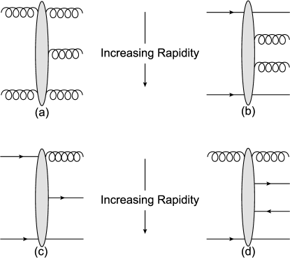
Figure 2: The particle flavour and momentum configurations in (a) and (b) allow the maximum number of $t$-channel gluon exchanges and so contribute at LL, while those in (c) and (d) require one $t$-channel quark-exchange and hence contribute at NLL.

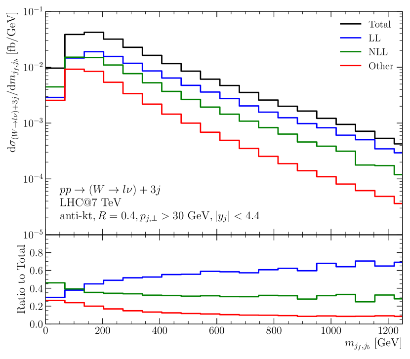
(a)

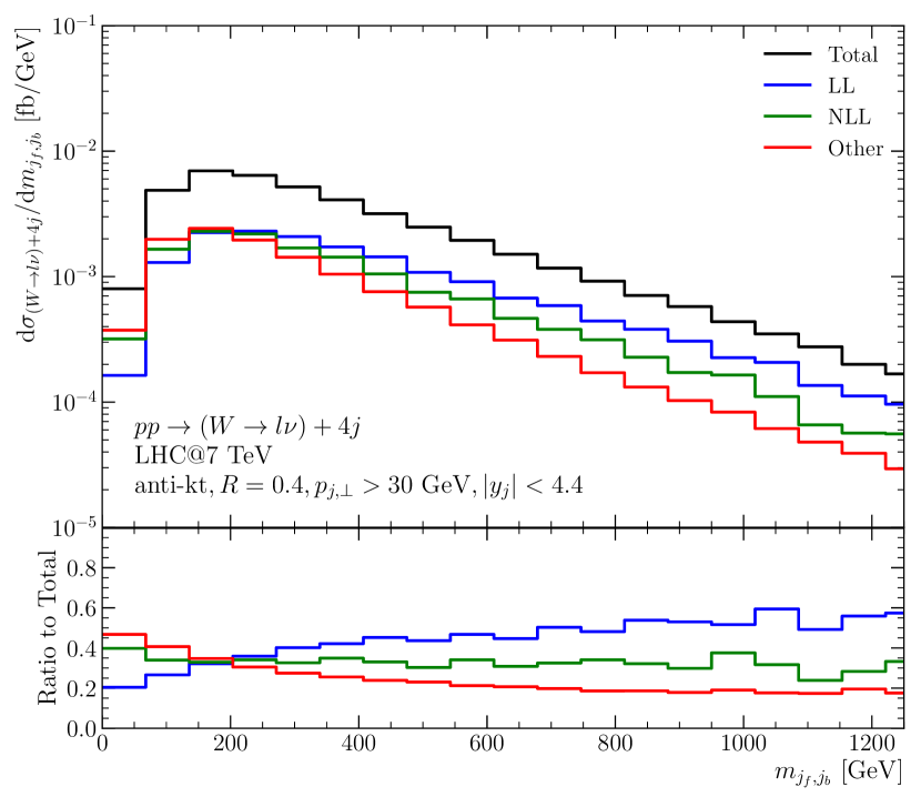
(b)

Figure 3: The leading order (a) $W+3$-jet and (b) $W+4$-jet cross sections as a function of the invariant mass between the most forward and backward jets, $m_{\rm fb}$. In addition to the total (black), we also show the split into the contributions from the LL configurations (blue), NLL configurations (green) and other configurations (red). As $m_{\rm fb}$ increases, the LL configurations increase in dominance but the NLL configurations remain significant.

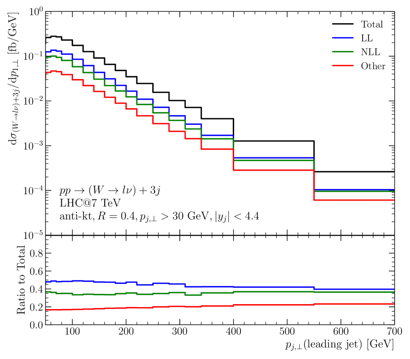
(a)

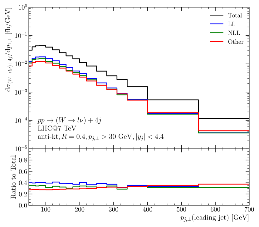
(b)

Figure 4: The leading order (a) $W+3$-jet and (b) $W+4$-jet cross sections as a function of the transverse momentum of the hardest jet, $p_{\perp,1}$. In addition to the total (black), we also show the split into the contributions from the LL configurations (blue), NLL configurations (green) and other configurations (red). As $p_{\perp,1}$ increases, the LL configurations decrease in importance underlining the importance of also applying resummation to the NLL contributions.

The importance of these NLL configurations may be demonstrated by considering contributions from LL and NLL configurations to the Born-level processes for $2\to 3$ and $2\to 4$. In fig. 3 we illustrate the differential distributions for (a) $W+3$-jet and (b) $W+4$-jet production as a function of the invariant mass between the most forward and backward jets, split into the LL component (blue), the NLL component (green) and other configurations (red). The results are all obtained using the full SM scattering amplitudes, and classifying the contributions according to the flavour and momentum configurations of the states, as summarised in table 1. These plots were made for 7 TeV proton-proton collisions and the jets were required to have $p_{\perp}>30$ GeV and $|y_{j}|<4.4$, but the behaviour is not sensitive to the details of such choices.

	LL processes	NLL processes
$pp\to W+3j$	$qg\to Wq^{\prime}gg$,	$qg\to Wgq^{\prime}g$, $qQ\to Wgq^{\prime}Q$,
	$qQ\to Wq^{\prime}gQ$	$gg\to Wq\bar{q}^{\prime}g$, $gQ\to Wq\bar{q}^{\prime}Q$, $gQ\to Wq\bar{q}Q^{\prime}$
$pp\to W+4j$	$qg\to Wq^{\prime}ggg$,	$qg\to Wgq^{\prime}gg$, $qQ\to Wgq^{\prime}gQ$, $qQ\to Wq^{\prime}gQg$,
	$qQ\to Wq^{\prime}ggQ$	$gg\to Wq\bar{q}^{\prime}gg$, $gQ\to Wq\bar{q}^{\prime}gQ$, $gQ\to Wq\bar{q}gQ^{\prime}$,
		$Qg\to WQ^{\prime}q\bar{q}g$, $Qg\to WQq\bar{q}^{\prime}g$, $gg\to Wgq\bar{q}^{\prime}g$,
		$Q\tilde{Q}\to WQ^{\prime}q\bar{q}\tilde{Q}$, $Q\tilde{Q}\to WQq\bar{q}^{\prime}\tilde{Q}$

Table 1: A summary of the particle configurations which enter the LL and NLL lines in fig. 3 and fig. 4. All particles except for the $W$ are listed in rapidity order. $q$, $Q$ etc. may refer to quarks or anti-quarks. Each process refers to itself and its symmetric counterpart, i.e. $qg\to Wq^{\prime}gg$ is shorthand for $qg\to Wq^{\prime}gg+gq\to Wggq^{\prime}$. All other subprocesses not listed above are included in the line labelled ”Other”.

As expected from arguments above, the LL configurations dominate as $m_{\rm fb}$ increases, while the relative contributions from the other configurations decrease. However, even at $m_{\rm fb}=1$ TeV, the sub-leading contributions still contribute roughly 30% in the $W+3$-jet case and almost 40% in the 4-jet case. A large $m_{\rm fb}$ is only part of the requirement of the MRK limit - indeed, large $m_{\rm fb}$ requires just one but not all invariant masses large.

The importance of accurately describing the NLL configurations is even more stark for transverse momentum distributions as $d\sigma/dp_{\perp,1}$, with $p_{\perp,1}$ the transverse momentum of the hardest jet, as in fig. 4. There is no correlation expected between the MRK limit (where the LL configurations will dominate) and the transverse momenta, and therefore there is no systematic suppression of sub-leading channels. In fact one sees that as $p_{\perp,1}$ increases, the contribution from sub-leading channels increases to 60% for $W+3$-jets and 70% for $W+4$-jet production.

Previously, the sub-leading channels had been included in the formalism of HEJ just through fixed-order matching; meaning that the NLL configurations of 3j and 4j channels did not receive the sophisticated all-order treatment of the LL channels. The all-order treatment of the NLL channels is made possible by the calculations presented in the current paper. As such, the all-order resummation will be applied to a large part of the total cross section, increasing from 40% to 80% in inclusive $W+3$-jet production, and from 30% to 70% in inclusive $W+4$-jet production.

This illustrates the importance of an effective description of NLL components, including all-order high-energy corrections, in order to improve the accuracy of the resummed predictions in sub-asymptotic regions of phase space. We will see that this leads to a much reduced dependence on fixed-order matching, and an improvement in our description of LHC data.

In order to set up the framework for the new calculations in section 3, we outline the structure of a HEJ amplitude in the next subsection.

2.2 High Energy Factorisation of the On-Shell Scattering Amplitudes

In the high energy limit of a $2\rightarrow n$ QCD partonic scattering process, namely where all partons are strongly ordered in rapidity, one finds that the matrix elements factorise into a product of expressions, each exhibiting dependence on a much reduced subset of external momenta DelDuca:1999ha . This factorisation holds even after the addition of a colour-singlet such as a Higgs, $W$ or a $Z/\gamma^{*}$ boson to the scattering.

In fact, a stronger statement than the one above can be made: the amplitude will factorise even if only a subset of the final state partons are strongly ordered in rapidity. The dependence of the amplitude upon partons obeying strong ordering will remain isolated in factors that remain simple, whereas the dependence upon partons where the rapidity-ordering condition is relaxed will appear in factors that are more complex and exhibit co-dependence on a greater number of external partons. Notably, if the strong ordering condition is relaxed between a pair of neighbouring partons, there will appear one less $t$-channel colour-octet propagator. This behaviour is illustrated in fig. 5, where the separation of the analytical expressions of the amplitude is also given in terms of unspecified functions $f$, $f_{i}$ and $g_{j}$. This motivates the concept of local momenta for each component, which is the relevant momentum subset within which there is no strong-rapidity ordering assumed.

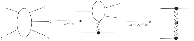
$i\mathcal{M}=\ f(p_{a},p_{b},p_{1},p_{2},p_{3})$,      $f_{1}(p_{a},p_{1},p_{2})f_{2}(p_{b},p_{3})$,        $g_{1}(p_{a},p_{1})g_{2}(q_{1},p_{2})g_{3}(p_{b},p_{3})$

Figure 5: In the limit that particles are well-separated in rapidity, QCD matrix elements factorise into independent pieces dependent only on a subset of momenta, as illustrated. This is true in the full high-energy limit where all particles are well-separated in rapidity (right-hand side), but also when the limit only applies to a subset of particles (middle).

The factorisation of the amplitude is extremely powerful because the kinematic dependence of external legs is isolated in only a small number of factors, which prevents a significant increase in complexity as the number of outgoing particles increases. This has the advantage that is easy to demonstrate that a minimal combination of components exhibit the scaling behaviour expected from eq. 7. Furthermore, the factorisation implies that the pieces are not only independent of the other momenta in the process, but also of the details of the rest of the process. In the example in fig. 5 it means that $f_{2}(p_{b},p_{3})=g_{3}(p_{b},p_{3})$ and in general means that components for high-multiplicity processes can be derived from low-multiplicity ones.

In Ref. DelDuca:1999ha , the factorised components of the amplitude (the impact factors) were derived in terms of scalar momentum components after these are approximated by their dominant components in the high-energy limit. In the HEJ formalism, we have found that using contractions of vector currents and tensors allows us to keep the required properties of factorisation, while making sufficiently few approximations so that HEJ amplitudes still satisfy Andersen:2009nu :

• gauge invariance in all phase space (not just in the high-energy limit),

• crossing symmetry between incoming and outgoing particles, and

• conservation of energy and momentum.

The fact that the factorised structure remains allows us to apply the resummation using the Lipatov Ansatz and generalisations of the Lipatov vertices used within BFKL descriptions Andersen:2009nu ; Andersen:2012gk . Specifically, in the HEJ formalism, the matrix element for a leading-log configuration $f_{a}f_{b}\to X+f_{a}\cdot ng\cdot f_{b}$ has the schematic form

$$\begin{split}\overline{\left|\mathcal{M}^{\rm HEJ,reg}_{f_{a}f_{b}\to Xf_{a}\cdot ng\cdot f_{b}}\right|}^{2}=&\ \mathcal{B}_{f_{a},f_{b},X}(p_{a},p_{b},p_{1},p_{n+2},\{p\}_{X})\\ &\ \cdot\prod_{i=1}^{n}\mathcal{V}(p_{a},p_{b},p_{1},p_{n+2},q_{i},q_{i+1})\\ &\ \cdot\prod_{j=1}^{n+1}\mathcal{W}(q_{j},y_{j},y_{j+1}).\end{split}$$ (16)

The first factor is the process-dependent Born-level function, $\mathcal{B}$, which does not depend on the momenta of any additional gluons which are produced. The notation $\{p\}_{X}$ represents the local momenta associated with the production of $X$, if present. This is then supplemented by vertex functions $\mathcal{V}$ for each of the $n$ additional gluons which depend on the momenta of the incoming and outermost outgoing particles, and the derived $t$-channel momentum $q_{i}$ defined as in fig. 1. The final factors, $\mathcal{W}$, represent the finite contribution from the combination of the virtual corrections and unresolved real emissions. There is one for each $q_{j}$ which depends only on that momentum and the rapidity difference between the emissions on either side. $\mathcal{V}$ and $\mathcal{W}$ are independent of the process-type (i.e. they are the same for all choices of $f_{a}$, $f_{b}$ and $X$).

In this paper, we will concentrate on the first of these factors, $\mathcal{B}$, where we derive new results. Our treatment of real and virtual corrections and the cancellation of the divergences between them (which leads to $\mathcal{V}$ and $\mathcal{W}$) is identical to previous studies and is implemented using the methods of HEJ 2 Andersen:2018tnm . Their analytic construction was first described in detail in Ref. Andersen:2011hs .

The function $\mathcal{B}$ is constructed as a contraction, $S$, of two “generalised currents” divided by corresponding $t$-channel momenta, written as the product $T_{X}$, and multiplied by suitable couplings and colour factors as follows:

$$\mathcal{B}_{f_{a},f_{b},X}(p_{a},p_{b},p_{1},p_{n+2},\{p\}_{X})=(g_{s}^{2})^{2}\ \frac{K_{f_{a}}K_{f_{b}}}{4(N_{C}^{2}-1)}\ ||S_{f_{a}f_{b}\to Xf_{a}\ldots f_{b}}||^{2}\ \frac{1}{T_{X}}.$$ (17)

As a simple example, in pure QCD ($X=0$), the spinor structure is just a helicity averaged contraction of two spinor currents,

$$S^{{h_{a},h_{b},h_{1},h_{n+2}}}_{f_{a}f_{b}\to f_{a}\ldots f_{b}}=\bar{u}^{h_{1}}(p_{1})\gamma^{\mu}u^{h_{a}}(p_{a})\ g_{\mu\nu}\ \bar{u}^{h_{n+2}}(p_{n+2})\gamma^{\nu}u^{h_{b}}(p_{b}),$$ (18)

where $h_{i}$ is the helicity of parton $i$. We use double-bar notation to write this quantity summed over all helicity combinations as

$$\left\|S_{f_{a}f_{b}\to f_{a}...f_{b}}\right\|^{2}=\sum_{\{h_{i}\}}|S^{{h_{a},h_{b},h_{1},h_{n+2}}}_{f_{a}f_{b}\to f_{a}\ldots f_{b}}(p_{1},p_{n+2},p_{a},p_{b})|^{2}.$$ (19)

The required $t$-channel momenta here are $T_{0}=t_{1}t_{n+1}$. The factors $K_{f_{i}}$ are colour factors which depend on the incoming particles. If $i$ is a quark, we simply have $K_{q}=C_{F}$. If $i$ is a gluon, we have a more involved factor depending on colour factors and the fraction of incoming light-cone momenta being carried by the most forward/backward gluon Andersen:2009he . In the strict high energy limit, we recover the result from BFKL, $K_{g}\rightarrow C_{A}$.

The function $\mathcal{B}$ is used to describe the production of hard perturbative particles and give a skeleton to which the other components are added. It would diverge in the limit that the momentum of one of the external partons (here $p_{1}$ or $p_{n+2}$) goes to zero as the formalism does not contain the corresponding virtual corrections for these (which would form part of the full next-to-leading logarithmic corrections). In order to enforce this important distinction between particles in $\mathcal{B}$ and particles produced via vertices in $\mathcal{V}$ in our event generator implementation, we require the outer partons to be part of the most forward/backward hard jet respectively, and to carry a significant fraction of the total jet momentum. The high-energy resummation is then applied to the phase space region between these two particles in rapidity.

In the rest of this section we discuss the construction of the function $\mathcal{B}$ for other processes, highlighting the features which will be important when we come to the new results in this paper.

2.3 Process-dependent Contractions of Effective Currents

The function $\mathcal{B}_{f_{a},f_{b},X}(p_{a},p_{b},p_{1},p_{n+2},\{p\}_{X})$ in eq. 16 represents the skeleton or Born process which is then supplemented with all-order high-energy resummation in HEJ. It takes the form shown in eq. 17 where the key component is the function, $S_{f_{a}f_{b}\to Xf_{1}\dots f_{2}}$. Using currents as described in section 2.2, we define the following general structure:

$$S_{f_{a}f_{b}\to Xf_{1}\dots f_{2}}=j^{h_{a},\dots,h_{1}}_{\mu}(p_{a},p_{1},\{p\}_{X})\ X^{\mu\nu}(\{p\}_{X})\ j^{h_{b},\dots,h_{n}}_{\nu}(p_{b},p_{n+2},\{p\}_{X}).$$ (20)

This spinor structure is sufficient to describe all existing HEJ processes and the new processes described in this paper. For example, we recover the pure QCD expressions given in eq. 18 by taking:

$$X^{\mu\nu}=g^{\mu\nu},\qquad j_{\mu}^{h}(\tilde{p},p)=\bar{u}^{h}(p)\gamma_{\mu}u^{h}(\tilde{p}).$$ (21)

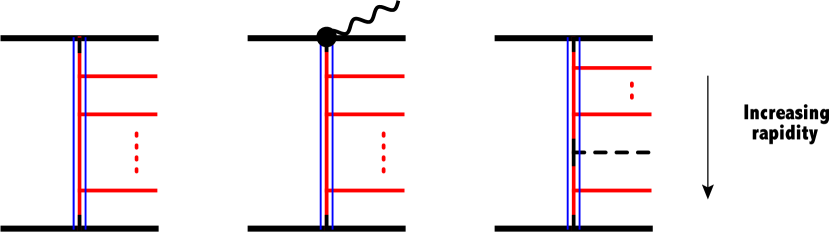
(a)                                  (b)                                  (c)

Figure 6: These diagrams illustrate the schematic structure of an amplitude in HEJ (eq. 16) for (a) pure jets, (b) $W$ plus jets and (c) Higgs boson plus jets. The black thick lines represent the skeleton or Born process in each case, described by the function $\mathcal{B}$. The external red lines represent the production of resolved real gluons, each with a factor $\mathcal{V}$. The blue lines indicate the range of rapidity over which the virtual corrections are applied, which are encoded in the $\mathcal{W}$ factors. Dotted red lines indicate that the number of additional gluons is not fixed and the dashed black line in (c) indicates the Higgs boson.

Figure 6(a) illustrates that the function $\mathcal{B}$ is used to describe the outer ends of the process (the parts represented by thick lines), while being independent of the exact structure in between. The resummation is applied between these ends in rapidity, illustrated by the thin blue lines. This is therefore the region where we may have an arbitrary number of resolved, real gluons, shown in red.

=

+

Figure 7: The $j_{W}$ current, section 2.3, is constructed from the two diagrams which contribute to the production of a $W$-boson from a given quark line.

The addition of an electroweak boson does not change the analysis of the scaling of multijet amplitudes given in eq. 7. Therefore, the leading-logarithmic contributions to $W$-plus-dijet production are FKL configurations of coloured particles and, in particular, the non-extremal partons are all gluons. The $W$ boson is therefore emitted from one of the extremal legs as in fig. 6(b). Without loss of generality, if it couples to the $p_{a}-p_{1}$ end of the chain, we find for $W\to\ell\bar{\ell}$

$$S_{f_{a}f_{b}\to Wf_{a}^{\prime}\dots f_{b}}=j_{W,\mu}(p_{a},p_{1},p_{\ell},p_{\bar{\ell}})\ g^{\mu\nu}\ j^{h_{b},\dots,h_{n}}_{\nu}(p_{b},p_{n+2})$$ (22)

where $j_{W,\mu}(p_{a},p_{1},p_{\ell},p_{\bar{\ell}})$ is the exact sum of the two contributions shown in  fig. 7:

$$j_{W}^{\mu}(p_{a},p_{1},p_{\ell},p_{\bar{\ell}})= \ \frac{g_{W}^{2}}{2}\ \frac{1}{p_{W}^{2}-M_{W}^{2}+i\ \Gamma_{W}M_{W}}\ \bar{u}^{-}(p_{\ell})\gamma_{\alpha}v^{-}(p_{\bar{\ell}})$$

$$\cdot\left(\frac{\bar{u}^{-}(p_{1})\gamma^{\alpha}(\not{p}_{1}+\not{p}_{W})\gamma^{\mu}u^{-}(p_{a})}{(p_{1}+p_{W})^{2}}+\frac{\bar{u}^{-}(p_{1})\gamma^{\mu}(\not{p}_{a}-\not{p}_{W})\gamma^{\alpha}u^{-}(p_{a})}{(p_{a}-p_{W})^{2}}\right).$$ (23)

The necessary components to form $\mathcal{B}$ in eq. 17 are then:

$$\begin{split}||S_{f_{a}f_{b}\to Wf_{a}^{\prime}...f_{b}}||^{2}&=\sum_{h_{b}=h_{n+2}}\left|j_{W}^{\mu}(p_{a},p_{\ell},p_{\bar{\ell}},p_{1})j_{\mu}^{h_{b}}(p_{b},p_{n+2})\right|^{2},\\ T_{W}&=q_{1}^{2}q_{n+1}^{2}=(p_{a}-p_{1}-p_{\ell}-p_{\bar{\ell}})^{2}(p_{b}-p_{n+2})^{2}.\end{split}$$ (24)

No approximation has been made in the Born process and hence this gives the exact expression for the $2\to 2$ amplitude. For certain combinations of initial quark flavours, it may be possible for a $W$ boson to be emitted from either end of the chain. Both are sampled within HEJ. The interference between the two is suppressed by both kinematic and flavour effects and hence is neglected.

The structure above is easily extended. The treatment of $Z/\gamma^{*}$-plus-dijet production is very similar to $W$-plus-dijet production with additional helicities and interference effects included Andersen:2016vkp . The description of Higgs-boson-plus-dijet production is described in detail in Andersen:2017kfc ; Andersen:2018kjg and is the first application where the tensor $X^{\mu\nu}$ is non-trivial, as illustrated in fig. 6(c), where the black Higgs vertex in the middle of the red region of resummation forms part of $\mathcal{B}$.

In this section, we have described the HEJ construction of all leading-logarithmic contributions in $\hat{s}/p_{\perp}^{2}$ to inclusive $W$-plus-dijet production. In the next section we present the calculation of the new components required to describe the well-defined subset of the next-to-leading-logarithmic contributions which we have identified as the most important to improve the description away from the strict high-energy limit.

3 Amplitudes for Subleading Processes

In the previous section we have outlined the construction of the necessary amplitudes to describe the leading-logarithmic contributions in $\hat{s}/p_{t}^{2}$ to inclusive $(X+)$-dijet processes within the HEJ framework. In this section we present our new calculations which provide the necessary components to calculate the leading-logarithmic contribution for all $W+3$-jet and $W+4$-jet subprocesses which contribute at next-to-leading log level to the inclusive $W+$dijet cross section. Until now, these processes have been included in HEJ only through matching to fixed order without any further all-order corrections. These new results therefore allow all-order high-energy resummation to be applied to a much larger fraction of the total cross section and significantly reduce the dependence of the HEJ predictions on fixed-order matching. We illustrate the numerical impact of these new components in section 3.3, after presenting the new calculations in sections 3.1 and 3.2.

3.1 New NLL Components: Inclusive 3-jet Processes

We are seeking to describe the leading-logarithmic terms of subprocesses whose particle flavour and momentum configurations give next-to-leading logarithmic contributions to the inclusive cross section. This means that at the level of the matrix-element-squared, their contribution should be suppressed by one power of $s_{ij}$ compared to the leading-logarithmic channels. The scaling behaviour in eq. 7 then implies that we need to describe processes with one less effective $t$-channel exchange of a gluon than the maximum number. An example of such a process is to take a LL configuration and swap the rapidity order of an outgoing quark and the gluon next to it, to give a single quark in the $t$-channel, as shown for 3 partons in fig. 2(c). In the rest of this section, we derive the necessary components to describe all 3-jet subprocesses which contribute at this order.

We take the following $W+3$-jet process as the first new case:

$$q(p_{a})Q(p_{b})\longrightarrow(W\to)\ell(p_{\ell})\bar{\ell}(p_{\bar{\ell}})g(p_{1})q^{\prime}(p_{2})Q(p_{3}),$$ (25)

where as usual we order $y_{1}<y_{2}<y_{3}$, and we take $q,q^{\prime},Q$ to be different quark flavours such that the vertex $q\to q^{\prime}W$ exists for a choice of sign for the $W$ charge. If we apply strong rapidity ordering among all particles, eq. 7 gives the following scaling of the amplitude in the MRK limit:

$$\mathcal{M}\sim(s_{12})^{1/2}(s_{23})^{1}\gamma.$$ (26)

This is suppressed by a half power of $s_{12}$ compared to the LL configuration where $y_{q^{\prime}}<y_{g}$, leading to an NLL contribution to the inclusive dijet cross section as required. We stress that for this particle assignment and configuration it is the LL contribution. This scaling argument holds whenever we have an LL configuration up to a single gluon produced backward of a quark or a single gluon produced forward of a quark; we refer to such a process as production of an ‘unordered’ gluon.

We remove the requirement of strong ordering between $p_{1}$ and $p_{2}$, but keep it for the other colour-charged particles: $y_{1},y_{2}\ll y_{3}$, as in the middle diagram of fig. 5. This is an example of Quasi-Multi Regge Kinematics (QMRK), where strong rapidity ordering is only enforced in a subset of particles. In this case, the scaling with $s_{12}$ is not prescribed (nor is that invariant necessarily large), and the scaling depends only on the invariants which are still controlled by strong ordering, in this case $s_{23}$. We expect the factorised structure to follow that of fig. 5. A new feature of the $j_{W{\rm uno}}$ current is that it must allow for different colour structures as the outgoing gluon and $t$-channel gluon may occur in either order. We therefore now write the colour matrix for the non-gluon end explicitly and expect the spinor structure within the corresponding skeleton function $\mathcal{B}_{qQW}^{\rm unoW}$ should now be

$$S_{qQ\to Wgq^{\prime}Q}^{\rm unoW}=j_{W{\rm uno}\,\mu}^{d}(p_{a},p_{1},p_{2},p_{\ell},p_{\bar{\ell}})\ g^{\mu\nu}\ T^{d}_{3b}\ j^{h_{b},h_{3}}_{\nu}(p_{b},p_{3}),$$ (27)

where $j_{\nu}^{h_{b},h_{3}}$ is the same current as the QCD process, eq. 21 and $T^{m}_{ij}$ represents fundamental colour matrices between quark state $i$ and $j$ with adjoint index $m$. The new current, $j^{d}_{W{\rm uno}}$, is non-zero only for the left-handed helicities $h_{a}=h_{1}=-$ and hence we have suppressed its helicity indices. It is derived from the sum of all leading-order Feynman diagrams for the process given in eq. 25. A factorised form can be obtained by dropping the terms kinematically suppressed in the QMRK limit; full details are given in section B.1. We find

$$\begin{split}j^{d\,\mu}_{W\rm uno}(p_{a},p_{1},p_{2},p_{\ell},p_{\bar{\ell}})=&\ -i\varepsilon_{\nu}(p_{1})\ \bar{u}^{-}(p_{\ell})\gamma_{\rho}v^{-}(p_{\bar{\ell}})\\ &\quad\times\ \left(T^{1}_{2i}T^{d}_{ia}(\tilde{U}_{1}^{\nu\mu\rho}-\tilde{L}^{\nu\mu\rho})+T^{d}_{2i}T^{1}_{ia}(\tilde{U}_{2}^{\nu\mu\rho}+\tilde{L}^{\nu\mu\rho})\right),\end{split}$$ (28)

where expressions for $\tilde{U}_{1,2}^{\nu\mu\rho}$ and $\tilde{L}^{\nu\mu\rho}$ may be found in eqs. 69, 72 and 80. It is straightforward to check that the Ward identity for the external gluon is satisfied as the tensors obey

$$p_{1\nu}\tilde{L}^{\nu\mu\rho}=p_{1\nu}\tilde{U}_{1}^{\nu\mu\rho}=-p_{1\nu}\tilde{U}_{2}^{\nu\mu\rho}.$$ (29)

The resulting amplitude is therefore gauge invariant in all of phase space, and not only in the QMRK limit. In the derivation, approximations are only made to the values of the momenta at the opposite end ($p_{b}$ and $p_{3}$). This increases the region of validity of the expression, but more than that, means that the approximations made are so minimal that crossing symmetry between initial and final states is preserved at the level of the derived currents, which we return to below.

We define the following contractions:

$$\begin{split}\tilde{X}&=\varepsilon^{h_{1}}_{\nu}(p_{1})\ \left[\bar{u}^{-}(p_{\ell})\gamma_{\rho}v^{-}(p_{\bar{\ell}})\right]\big{[}\bar{u}^{h_{3}}(p_{3})\gamma_{\mu}^{h_{b}}(p_{b})\big{]}\left(\tilde{U}_{1}^{\nu\mu\rho}-\tilde{L}^{\nu\mu\rho}\right),\\ \tilde{Y}&=\varepsilon^{h_{1}}_{\nu}(p_{1})\ \left[\bar{u}^{-}(p_{\ell})\gamma_{\rho}v^{-}(p_{\bar{\ell}})\right]\big{[}\bar{u}^{h_{3}}(p_{3})\gamma_{\mu}^{h_{b}}(p_{b})\big{]}\left(\tilde{U}_{2}^{\nu\mu\rho}+\tilde{L}^{\nu\mu\rho}\right).\end{split}$$ (30)

Then, from eq. 28, the final HEJ expression for the tree-level process $qQ\to e\nu_{e}gq^{\prime}Q$ is

$$\left|\overline{\mathcal{M}_{qQ\to Wgq^{\prime}Q}^{{\tt HEJ}\ \rm{tree}}}\right|^{2}=g_{s}^{6}\frac{C_{F}^{2}}{4(N_{C}^{2}-1)}\frac{\left\|S_{qQ\to Wgq^{\prime}Q}^{\rm uno}\right\|^{2}}{(p_{a}-p_{1}-p_{2}-p_{\ell}-p_{\bar{\ell}})^{2}(p_{b}-p_{3})^{2}},$$ (31)

where

$$\begin{split}\left\|S_{qQ\to Wgq^{\prime}Q}^{\rm unoW}\right\|^{2}&=\sum_{h_{b},h_{3},h_{1}}\ \bigg{[}C_{F}|\tilde{X}+\tilde{Y}|^{2}-C_{A}\,{\rm Re}(\tilde{X}\tilde{Y}^{*})\bigg{]}.\end{split}$$ (32)

We now wish to derive our skeleton function $\mathcal{B}_{qQW}^{\rm unoW}$ for this process, to be used to describe the process above with an arbitrary number of additional gluons (analogous to e.g. eq. 17). In our formalism, it is valid to apply resummation over the range of rapidity where strong rapidity ordering is applied. In this example, eq. 25, that is the range $[y_{2},y_{3}]$. This will be the region where real gluons (governed by vertex functions $\mathcal{V}$) and virtual corrections (governed by exponential factors $\mathcal{W}$) are applied, and so at all orders leads to the structure shown in fig. 8(a).

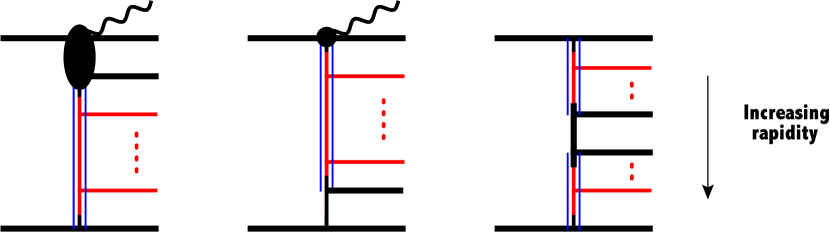
(a)                                  (b)                                  (c)

Figure 8: These diagrams illustrate the resummation structure of the new processes we describe after the calculation of the new components in this section: (a) $qQ\to(W\to)\ell\bar{\ell}gq^{\prime}\ldots Q$, (b) $qQ\to(W\to)\ell\bar{\ell}q^{\prime}\ldots Qg$ and (c) $qQ\to q\ldots\tilde{q}\bar{\tilde{q}}\ldots Q$. The thick black lines show the components described by the skeleton function $\mathcal{B}$ and the external red lines indicate possible real gluons. The blue lines show the region where strong ordering and therefore resummation is applied. The decay products of the $W$ have been omitted for clarity.

For the process with $n$ coloured outgoing particles (i.e. $(n-3)$ additional real gluons between the quarks):

$$q(p_{a})f_{b}(p_{b})\to(W\to)\ell(p_{\ell})\bar{\ell}(p_{\bar{\ell}})\ g(p_{1})q^{\prime}(p_{2})\ldots g(p_{i})\ldots f_{b}(p_{n}),$$ (33)

we then define the following skeleton function

$$\begin{split}\mathcal{B}_{qQW}^{\rm unoW}=&g_{s}^{6}\frac{C_{F}K_{f_{b}}}{4(N_{C}^{2}-1)}\ \frac{1}{q_{2}^{2}q_{n-1}^{2}}\left\|S_{qf_{b}\to Wgq^{\prime}\ldots f_{b}}^{\rm unoW}\right\|^{2},\\ q_{2}=&p_{a}-p_{\ell}-p_{\bar{\ell}}-p_{1}-p_{2},\qquad q_{i}=q_{i-1}-p_{i},\ i>2\\ \left\|S_{qf_{b}\to Wgq^{\prime}\ldots f_{b}}^{\rm unoW}\right\|^{2}&=\sum_{h_{b},h_{n},h_{1}}\ \bigg{[}C_{F}|\tilde{X}+\tilde{Y}|^{2}-C_{A}\,{\rm Re}(\tilde{X}\tilde{Y}^{*})\bigg{]},\end{split}$$ (34)

where the mapping $p_{3}\to p_{n}$ is made within $\tilde{X}$ and $\tilde{Y}$. The tree-level factor of $1/(p_{b}-p_{3})^{2}$ has been generalised to $1/q_{n-1}^{2}$; as in the LL processes in section 2.3, we do this symmetrically to match the factors of $1/q_{i}^{2}$ in our prescription for real gluon vertices. When $n=3$ and $f_{b}$ is a quark, eq. 34 reproduces the tree-level result of eq. 31. As before, $\mathcal{B}_{qQW}^{\rm unoW}$ represents the underlying skeleton process and therefore each outgoing coloured particle will be required to be hard in the perturbative sense (implemented by requiring each parton to contribute a significant fraction of momentum to its own jet, not containing another skeleton parton).

As our second process, we consider

$$q(p_{a})Q(p_{b})\longrightarrow(W\to)\ell(p_{\ell})\bar{\ell}(p_{\bar{\ell}})q^{\prime}(p_{1})Q(p_{2})g(p_{3}).$$ (35)

Like the process above, this has a $W$ produced from a quark line and an unordered gluon, but these are now produced from different quark lines. If there was strong ordering between $p_{2}$ and $p_{3}$, the effective $t$-channel particle between them would be a quark. The effective $t$-channel between $p_{1}$ and $p_{2}$ is still a gluon, so we expect $\mathcal{M}\sim(s_{12})^{1}(s_{23})^{1/2}$. This is therefore the same logarithmic order as the first example in this section. We will now relax the requirement between $p_{2}$ and $p_{3}$ such that the relevant QMRK limit is now $y_{1}\ll y_{2},y_{3}$. We therefore expect the spinor structure to take the form

$$S_{qQ\to Wq^{\prime}Qg}^{\rm uno}=j_{W\,\mu}(p_{a},p_{1},p_{\ell},p_{\bar{\ell}})T^{d}_{1a}\ g^{\mu\nu}\ j_{{\rm uno}\,\nu}^{d\,h_{b},h_{2},h_{3}}(p_{b},p_{2},p_{3}).$$ (36)

The factorisation of amplitudes in the high-energy limit dictates that $j_{{\rm uno}\,\nu}^{d}$ is independent of the $W$ boson and, indeed, of the rest of the process. It is therefore the same unordered current that we find in the pure jet process and in Higgs boson plus dijets. This was given in Ref. Andersen:2017kfc :

$$j^{d,h_{b},h_{2},h_{3}\,\mu}_{\rm uno}(p_{b},p_{2},p_{3})=-i\varepsilon_{\nu}(p_{3})\left(T^{3}_{2i}T^{d}_{ia}\left(U_{1}^{\mu\nu}-L^{\mu\nu}\right)+T^{d}_{2i}T^{3}_{ia}\left(U_{2}^{\mu\nu}+L^{\mu\nu}\right)\right),$$ (37)

with $U_{1,2}^{\mu\nu}$ and $L^{\mu\nu}$ given in eq. 83. The colour structure is equivalent to the previous case, as we should expect. Again it is easily checked that this current also satisfies gauge invariance in all of phase space. One can derive the known scalar expression for the BFKL NLO impact factor DelDuca:1999ha from eq. 37 by taking the further approximations used in that paper.

The resummation pattern of this subprocess is shown in fig. 8(b). The construction of the skeleton function $\mathcal{B}_{qQW}^{\rm uno}$ allowing for $(n-3)$ extra gluons between the quarks follows the same pattern as the previous case, eq. 34. After defining,

$$X =\varepsilon^{h_{n}}_{\nu}(p_{n})\ j_{W\,\mu}(p_{a},p_{\ell},p_{\bar{\ell}},p_{1})\left(U_{1}^{\mu\nu}-L^{\mu\nu}\right),$$ (38)

$$Y =\varepsilon^{h_{n}}_{\nu}(p_{n})\ j_{W\,\mu}(p_{a},p_{\ell},p_{\bar{\ell}},p_{1})\left(U_{2}^{\mu\nu}+L^{\mu\nu}\right).$$ (39)

we find

$$\begin{split}\mathcal{B}_{qQW}^{\rm uno}=&g_{s}^{6}\frac{C_{F}^{2}}{4(N_{C}^{2}-1)}\left\|S_{qQ\to Wq^{\prime}\ldots Qg}^{\rm uno}\right\|^{2}\ \frac{1}{q_{1}^{2}q_{n-2}^{2}},\\ q_{1}=&p_{a}-p_{1}-p_{\ell}-p_{\bar{\ell}},\qquad q_{i}=q_{i-1}-p_{i},\ i\geq 2\\ \left\|S_{qQ\to Wq^{\prime}\ldots Qg}^{\rm uno}\right\|^{2}&=\sum_{h_{b},h_{n-1},h_{n}}\ \bigg{[}C_{F}|X+Y|^{2}-C_{A}\,{\rm Re}(XY^{*})\bigg{]},\end{split}$$ (40)

with the substitution $p_{2}\to p_{n-1}$ and $p_{3}\to p_{n}$ in $X$ and $Y$. Resummation is again applied over the range of strong ordering, which in this case is $[y_{1},y_{n-1}]$, as illustrated in fig. 8(b).

We note in passing that we may deduce the equivalent pure jet process without a $W$ boson, $q(p_{a})Q(p_{b})\to q(p_{1})Q(p_{2})g(p_{3})$ by replacing $j_{W}$ in eq. 36 with a quark current:

$$S^{\rm uno}_{qQ\to qQg}=j_{\mu}(p_{a},p_{1})T^{d}_{1a}g^{\mu\nu}j_{{\rm uno}\nu}^{d\,h_{b},h_{2},h_{3}}(p_{b},p_{2},p_{3}).$$ (41)

The construction of the suitable $\mathcal{B}^{\rm uno}_{qQ}$ function is analogous to eq. 40.

For our third and fourth processes at this order, we consider $W+3$-jet channels with a gluon in the incoming state. At leading log, an incoming gluon implies that the corresponding extremal outgoing particle must also be a gluon to give the necessary gluon in the effective $t$-channel. For the NLL contributions considered in this section, that restriction no longer applies. Our first example of this type is where an incoming gluon splits into an outgoing $\bar{q}q^{\prime}$ pair and a $W$ boson, e.g.

$$g(p_{a})Q(p_{b})\to(W\to)\ell(p_{\ell})\bar{\ell}(p_{\bar{\ell}})\bar{q}(p_{1})q^{\prime}(p_{2})Q(p_{3}).$$ (42)

In strong rapidity ordering, there would be an effective $t$-channel quark between $p_{1}$ and $p_{2}$ giving the suppression of $(s_{12})^{1/2}$ seen in the previous processes in this section. In the QMRK, $y_{1},y_{2}\ll y_{3}$, we apply resummation over the region of strong ordering $[y_{2},y_{3}]$ as shown in fig. 8(a). At leading-order, there exists crossing symmetry between this process and the process in eq. 25, under $p_{a}\leftrightarrow p_{1}$. In the derivation of the $j^{d\,\mu}_{W{\rm uno}}$ current for that process, approximations were only made to $p_{b}$ and $p_{3}$, and therefore this crossing symmetry persists at the level of the currents in HEJ amplitudes. We therefore find

$$j^{d\,\mu}_{Wq\bar{q}^{\prime}}(p_{a},p_{1},p_{2},p_{\ell},p_{\bar{\ell}})=j^{d\,\mu}_{W{\rm uno}}(p_{1},p_{a},p_{2},p_{\ell},p_{\bar{\ell}}).$$ (43)

The full skeleton $\mathcal{B}^{\rm extW}_{gW}$ is then constructed as in eq. 34.

Finally we consider the case with an incoming gluon splitting into a $q\bar{q}$ pair, where now the $W$ is produced from the other quark line:

$$q(p_{a})g(p_{b})\to(W\to)\ell(p_{\ell})\bar{\ell}(p_{\bar{\ell}})q^{\prime}(p_{1})Q(p_{2})\bar{Q}(p_{3}).$$ (44)

This is related by crossing symmetry to the process given in eq. 35 under $p_{b}\leftrightarrow p_{3}$ such that one can derive

$$j_{q\bar{q}}^{d\,h_{b},h_{2},h_{3},\mu}(p_{b},p_{2},p_{3})=j_{\rm uno}^{d\,h_{3},h_{2},h_{b}\,\mu}(p_{3},p_{2},p_{b}).$$ (45)

This is then contracted with a $W$ current at the opposite end, as indicated by the structure in fig. 8(b), to give the following spinor structure

$$S_{qg\to Wq^{\prime}\ldots Q\bar{Q}}^{\rm ext}=j_{W\,\mu}(p_{a},p_{1},p_{\ell},p_{\bar{\ell}})T^{d}_{1a}\ g^{\mu\nu}\ j_{q\bar{q}\,\nu}^{d,h_{b},h_{2},h_{3}}(p_{b},p_{2},p_{3}).$$ (46)

The skeleton function $\mathcal{B}^{\rm ext}_{gW}$ is then constructed as in eq. 40. From here, as for the production of an unordered gluon, one can immediately deduce the corresponding process in three-jet production without a $W$ boson, $q(p_{a})g(p_{b})\to q(p_{1})Q(p_{2})\bar{Q}(p_{3})$, by replacing $j_{W}(p_{a},p_{1},p_{\ell},p_{\bar{\ell}})$ with $j(p_{a},p_{1})$.

We now wish to illustrate that the new components we have derived do indeed give the correct scaling for the matrix-element in the full MRK limit. We will also compare these approximate HEJ skeleton amplitudes (i.e. without resummation) to leading-order results taken from MadGraph5_aMC@NLO Alwall:2014hca , to illustrate the quality of the approximation.

For our first subleading channels with an unordered gluon, in the MRK limit we should have (see eq. 26):

$$\left|\overline{\mathcal{M}_{qQ\to Wgq^{\prime}Q}^{{\tt HEJ}\ \rm{tree}}}\right|^{2}\sim s_{12}s^{2}_{23}\gamma$$ (47)

where again $\gamma$ is a finite function of transverse momentum. In the MRK limit, this scaling is equivalent to:

$$\left|\overline{\mathcal{M}_{qQ\to Wgq^{\prime}Q}^{{\tt HEJ}\ \rm{tree}}}\right|^{2}\times\frac{s_{12}}{\hat{s}^{2}}\rightarrow\mathrm{finite\ const}.$$ (48)

We illustrate this behaviour in fig. 9(a) for $qQ\rightarrow e\nu_{e}gq^{\prime}Q$ (eq. 25). The parameter $\Delta$ parameterises the rapidity separation between the coloured particles, as we have chosen $y_{1}=-\Delta$, $y_{2}=0$ and $y_{3}=\Delta$, see appendix A for the exact parameters.

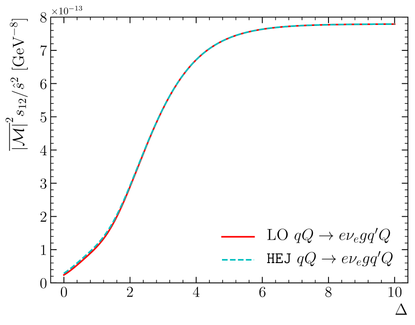
(a)

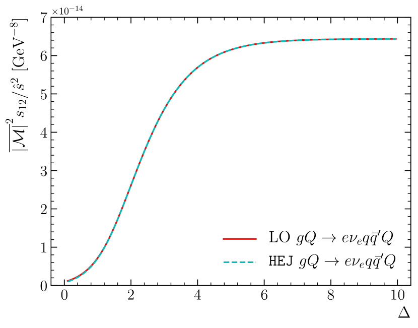
(b)

Figure 9: Plots illustrating the scaling of the HEJ approximation at tree-level to the matrix elements (cyan, dashed) for (9(a)) $qQ\rightarrow e\nu_{e}gq^{\prime}Q$, and (9(b)) $gQ\rightarrow e\nu_{e}q\bar{q}^{\prime}Q$. The parameter $\Delta$ represents the rapidity separation of the coloured particles as described in the text. Also shown is the leading order result (red, solid). Both cases are seen to obey the expected scaling, eq. 48, and further to give a good description of the full LO matrix element across the whole range.

We can see that the quantity $\overline{|\mathcal{M}|}^{2}\hat{s}_{12}/\hat{s}^{2}$ does indeed tend to a non-zero, finite constant at large values of $\Delta$. Moreover, the HEJ approximation describes the full leading-order result well across the entire phase space, deviating only slightly at the lowest values of $\Delta$. This is a consequence of the minimality of the approximation made in the derivation.

In fig. 9(b), we show the equivalent plots for the subprocess $gQ\rightarrow e\nu_{e}q\bar{q}^{\prime}Q$ (eq. 42). The jets have rapidities as in fig. 9(a) such that large values of $\Delta$ represent the MRK limit. It is again clear that the expected scaling is seen as both lines approach a non-zero finite constant. Moreover, the approximations in the skeleton HEJ process give an extremely good description of the leading-order matrix element for all values of $\Delta$. This would not have been the case if the strict limit was applied in all phase space.

3.2 New NLL Components: Inclusive 4-Jet Processes

In the previous section, we calculated all the components which are necessary to calculate the leading logarithmic components of all 3-jet subprocesses which contribute at next-to-leading log to the inclusive $W+3$-jet cross section. This automatically includes many of the processes which are necessary to do the same for $W+4$jets. For example, the process

$$q(p_{a})Q(p_{b})\longrightarrow(W\to)\ell(p_{\ell})\bar{\ell}(p_{\bar{\ell}})g(p_{1})q^{\prime}(p_{2})g(p_{3})Q(p_{4}),$$ (49)

is given in HEJ by:

$$\overline{\left|\mathcal{M}^{{\tt HEJ}\ \rm{tree}}_{qQ\to Wgq^{\prime}gQ}\right|}^{2}=\ \mathcal{B}_{qQW}(p_{a},p_{b},p_{1},p_{2},p_{4},p_{\ell},p_{\bar{\ell}})\cdot\mathcal{V}(p_{a},p_{b},p_{1},p_{4},q_{1},q_{2}),$$ (50)

where $\mathcal{B}_{qQW}(p_{a},p_{b},p_{1},p_{2},p_{4},p_{\ell},p_{\bar{\ell}})$ has already been given in eq. 34 for the $W+3$-jet process. This easily generalises further to 5, 6 or more jets. Similarly, one can approximate the other unordered gluon processes and incoming gluon to quark-anti-quark processes using the results already derived in section 3.1, by taking the relevant function $\mathcal{B}$ and multiplying by the required number of vertices $\mathcal{V}$.

There is just one further class of subprocess which formally contributes at NLL. This is where a $q\bar{q}$ pair is produced in the middle of the rapidity chain, potentially accompanied by a $W$ boson, see fig. 10. This differs from the processes in section 3.1 because the extremal ends of the chain are as in the LL case, but we must now derive a new piece to describe particles which are intermediate in rapidity. The structure of the resummation is as shown in fig. 8(c). As the figure suggests, we do not modify either of the currents in eq. 17, but instead alter the contraction between them, $X^{\mu\nu}$. We will find that this also needs to carry two colour indices, $d$ and $e$.

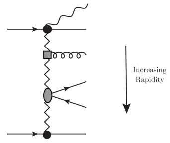
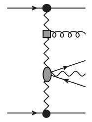
(a)                                        (b)                      a

Figure 10: Two processes which contribute at next-to-leading log and are relevant for four jets and above: (a) $q\tilde{q}\to Wq^{\prime}gQ\bar{Q}\tilde{q}$ in that rapidity order which contains a central $Q\bar{Q}$ pair and $W$ produced from a different quark line, and (b) $q\tilde{q}\to qgQ\bar{Q}^{\prime}W\tilde{q}$ in that rapidity order where the $W$ is produced from the central $Q\bar{Q}^{\prime}$-pair. The rapidity-ordering applies to the coloured particles and not to the $W$ boson or its decay products.

We will derive the necessary tensors, $X^{de\,\mu\nu}_{{\rm cen}}(p_{2},p_{3},q_{1},q_{3})$ and $X^{de\,\mu\nu}_{{\rm cen}W}(p_{2},p_{3},p_{\ell},p_{\bar{\ell}},q_{1},q_{3})$, by considering the lowest order processes where they occur. For the case where the $W$ is produced from an outer quark line, we may exploit amplitude factorisation to derive the central $Q\bar{Q}$ tensor from a process without a $W$ boson:

$$q(p_{a})\ \tilde{q}(p_{b})\ \longrightarrow\ q(p_{1})\ Q(p_{2})\ \bar{Q}(p_{3})\ \ \tilde{q}(p_{4}).$$ (51)

For the case where the $W$ is produced from the central $Q\bar{Q}$ pair, we use

$$q(p_{a})\ \tilde{q}(p_{b})\ \longrightarrow\ q(p_{1})\ Q(p_{2})\ \bar{Q^{\prime}}(p_{3})\ (W\to)\ell(p_{\ell})\bar{\ell}(p_{\bar{\ell}})\ \tilde{q}(p_{4}).$$ (52)

As the new central $Q\bar{Q}$ piece contains the quark propagator, we will treat this as part of the skeleton process, as illustrated in fig. 8(c). This means that we do not impose strong ordering between the $Q\bar{Q}$-pair and take the following rapidity limit for the coloured particles:

$$y_{1}\ll y_{2},y_{3}\ll y_{4}.$$ (53)

In fact we also do not impose ordering between $y_{2}$ and $y_{3}$ so the same results apply if the anti-quark in the $Q\bar{Q}$-pair is backward of the quark. In this limit, we expect the matrix elements corresponding to eq. 51 and eq. 52 to take the forms:

$$i\mathcal{M}_{\rm cen} =g_{s}^{4}T^{d}_{1a}T^{e}_{4b}\ \frac{j_{\mu}(p_{a},p_{1})\ X^{de\,\mu\nu}_{{\rm cen}}(p_{2},p_{3},q_{1},q_{3})\ j_{\nu}(p_{b},p_{4})}{t_{a1}t_{b4}}$$ (54)

$$i\mathcal{M}_{\rm cenW} =g_{s}^{4}T^{d}_{1a}T^{e}_{4b}\ \frac{j_{\mu}(p_{a},p_{1})\ X^{de\,\mu\nu}_{{\rm cen}W}(p_{2},p_{3},p_{\ell},p_{\bar{\ell}},q_{1},q_{3})\ j_{\nu}(p_{b},p_{4})}{t_{a1}t_{b4}}.$$ (55)

We sum together all leading-order diagrams in each process and after applying the QMRK limit (eq. 53), we find (see sections C.1 and C.2):

$$\begin{split}X^{de\,\mu\nu}_{\rm cen}&=iT^{d}_{2q}T^{e}_{q3}\left[X_{s}^{\mu\nu}+X^{\mu\nu}_{6}\right]-iT^{e}_{2q}T^{d}_{q3}\left[X_{s}^{\mu\nu}+X^{\mu\nu}_{7}\right],\end{split}$$ (56a)

$$\begin{split}X^{de\,\mu\nu}_{{\rm cen}W}&=iT^{d}_{2q}T^{e}_{q3}\left[\tilde{X}_{s}^{\mu\nu}+\tilde{X}_{6}^{\mu\nu}\right]-iT^{e}_{2q}T^{d}_{q3}\left[\tilde{X}_{s}^{\mu\nu}+\tilde{X}^{\mu\nu}_{7}\right],\end{split}$$ (56b)

where $X_{s}^{\mu\nu}$, $X^{\mu\nu}_{6}$, $X^{\mu\nu}_{7}$, $\tilde{X}^{\mu\nu}_{s}$, $\tilde{X}^{\mu\nu}_{6}$ and $\tilde{X}^{\mu\nu}_{7}$ are defined in eqs. 95, 92, 106, 107 and 108. From eq. 54, the final summed and averaged matrix-element-squared for the central process without a $W$ boson is then given by

$$\begin{split}\overline{\left|M_{\ q\tilde{q}\to qQ\bar{Q}\tilde{q}}^{{\tt HEJ}\ \rm{tree}}\right|}^{2}&=\frac{1}{4C_{A}^{2}}\frac{g_{s}^{8}}{t_{a1}^{2}t_{b4}^{2}}\ \sum_{\left\{h_{i}\right\}}\left[C_{F}(|V|^{2}+|W|^{2})-\frac{1}{C_{A}}{\rm Re}(VW^{*})\right],\end{split}$$ (57)

where the sum runs over all allowed helicity combinations and the contracted current structures $V$ and $W$ are defined as

$$\begin{split}V&=j_{\mu}(p_{a},p_{1})\left(X_{s}^{\mu\nu}+X^{\mu\nu}_{6}\right)j_{\nu}(p_{b},p_{4}),\quad W=j_{\mu}(p_{a},p_{1})\left(X_{s}^{\mu\nu}+X^{\mu\nu}_{7}\right)j_{\nu}(p_{b},p_{4}).\end{split}$$ (58)

This easily describes the process we need with a $W$ boson produced from an outer quark line after replacing either $j_{\mu}(p_{a},p_{1})$ or $j_{\nu}(p_{b},p_{4})$ in eq. 58 with the $W$ current given in section 2.3. We may similarly adapt eq. 57 to describe the process where a $W$ boson is produced from a central $Q\bar{Q}^{\prime}$ pair by the simple replacement of $V$ and $W$ with

$$\begin{split}\widetilde{V}&=j_{\mu}(p_{a},p_{1})\left(\tilde{X}_{s}^{\mu\nu}+\tilde{X}^{\mu\nu}_{6}\right)j_{\nu}(p_{b},p_{4}),\quad\widetilde{W}=j_{\mu}(p_{a},p_{1})\left(\tilde{X}_{s}^{\mu\nu}+\tilde{X}^{\mu\nu}_{7}\right)j_{\nu}(p_{b},p_{4}).\end{split}$$ (59)

We now wish to demonstrate that this construction does indeed respect the correct scaling in the full MRK limit. Specifically, we should find (cf. eq. 48)

$$\frac{\overline{\left|M_{q\tilde{q}\to qQ\bar{Q}\tilde{q}}^{{\tt HEJ}\ \rm{tree}}\right|}^{2}s_{23}}{\hat{s}^{2}}\longrightarrow{\rm finite\ constant}\neq 0.$$ (60)

This scaling behaviour will be unaltered by the production of a $W$ boson from an outer quark or from the central $Q\bar{Q}$ pair. We illustrate this scaling for the process $q\tilde{q}\rightarrow e\nu_{e}qQ\bar{Q}^{\prime}\tilde{q}$ in fig. 11. We take a slice through phase space where the jets have the following rapidities

$$y_{1}=\Delta,\ y_{2}=\Delta/3,\ y_{3}=-\Delta/3,\,y_{4}=-\Delta,$$ (61)

such that the MRK limit is reached in the limit of large $\Delta$, see appendix A. It is clear that indeed the limit of eq. 60 is reached both in the HEJ approximation and in the full leading-order result. Furthermore, the HEJ approximation of the skeleton amplitude gives a very close approximation to the full leading-order result.

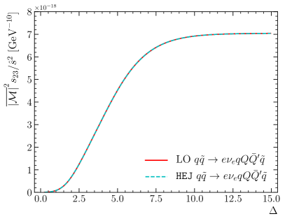
Figure 11: Plot illustrating the scaling of the HEJ approximation to the matrix element (cyan, dashed) for $q\tilde{q}\rightarrow e\nu_{e}qQ\bar{Q}^{\prime}\tilde{q}$. The parameter $\Delta$ represents the rapidity separation of the coloured particles as described in the text. Also shown is the leading order result (red, solid). We see that the expected scaling relation eq. 60 is obeyed, and that the HEJ approximation gives a good description of the full LO matrix element across the whole range of $\Delta$.

As before, we construct the required skeleton functions by generalising the corresponding matrix-element-squared to allow for the production of additional gluons. We again only apply our resummation over the regions of strong rapidity ordering, which in this case is the rapidity interval between the most forward and backward coloured particles minus the rapidity range between the quark and anti-quark. For the following process,

$$q(p_{a})f_{b}(p_{b})\to(W\to)\ell(p_{\ell})\bar{\ell}(p_{\bar{\ell}})\ q^{\prime}(p_{1})g(p_{2})\ldots g(p_{i-1})Q(p_{i})\bar{Q}(p_{i+1})g(p_{i+2})\ldots g(p_{n-1})f_{b}(p_{n}),$$ (62)

the resummation range is therefore the sum of $[y_{1},y_{i}]$ and $[y_{i+1},y_{n}]$, as illustrated in fig. 8(c). The skeleton function for this process is

$$\begin{split}\mathcal{B}_{\rm cen}&=g_{s}^{8}\frac{C_{F}K_{f_{b}}}{4(N_{c}^{2}-1)}\frac{1}{q_{1}^{2}q_{n-1}^{2}}\left\|S^{\rm cen}_{qf_{b}\to Wq^{\prime}\ldots Q\bar{Q}\ldots f_{b}}\right\|^{2},\\ \left\|S_{qf_{b}\to Wq^{\prime}\ldots Q\bar{Q}\ldots f_{b}}^{\rm cen}\right\|^{2}&=\frac{1}{2}\frac{1}{q_{i-1}^{2}q_{i+1}^{2}}\sum_{\{h_{i}\}}\ \left[C_{F}(|V|^{2}+|W|^{2})-\frac{1}{C_{A}}{\rm Re}(VW^{*})\right].\end{split}$$ (63)

This expression allows for the incoming particle $b$ to be a quark, anti-quark or gluon.

We follow the identical steps to construct the skeleton function for processes where the $W$ boson is produced from the central $Q\bar{Q}^{\prime}$ pair. In this case the skeleton function is given by

$$\begin{split}\mathcal{B}_{\rm cenW}&=g_{s}^{8}\frac{K_{f_{a}}K_{f_{b}}}{4(N_{c}^{2}-1)}\frac{1}{q_{1}^{2}q_{n-1}^{2}}\left\|S^{\rm cenW}_{f_{a}f_{b}\to f_{a}\ldots WQ\bar{Q}^{\prime}\ldots f_{b}}\right\|^{2},\\ \left\|S_{f_{a}f_{b}\to f_{a}\ldots WQ\bar{Q}^{\prime}\ldots f_{b}}^{\rm cenW}\right\|^{2}&=\frac{1}{2}\frac{1}{q_{i-1}^{2}q_{i+2}^{2}}\sum_{\{h_{i}\}}\ \left[C_{F}(|\widetilde{V}|^{2}+|\widetilde{W}|^{2})-\frac{1}{C_{A}}{\rm Re}(\widetilde{V}\widetilde{W}^{*})\right].\end{split}$$ (64)

Real and virtual all-order corrections are then added to eqs. 63 and 64 as in eq. 16 to give the full all-order HEJ amplitudes for these processes at any multiplicity.

3.3 Numerical Impact of New NLL Components

In figs. 3 and 4 in section 2.1, we presented a breakdown of the leading order cross-section for $pp\to(W\to\ell\nu)+3j$ and $pp\to(W\to\ell\nu)+4j$. The individual contributions were separated into leading-log (LL) configurations, next-to-leading-log (NLL) configurations and other (i.e. further suppressed) configurations and we saw that NLL contributions accounted for as much as 40% of the cross section in key areas of phase space. In the previous subsections, we have derived all of the necessary components to construct HEJ amplitudes for these NLL configurations, which then allows for an all-order resummation of the dominant high-energy effects to be applied to this part of the cross section too.

We will now illustrate the numerical impact of these new components in figs. 12–14. We plot the total differential cross-section and show its split into all-order and fixed-order components as follows:

• Case 1: The LO result plus all LL corrections ($\alpha_{s}^{2+k}\log^{k}(\hat{s}/p_{t}^{2})$) are included. This is plotted in panel (a) of figs. 12–14. Resummation is therefore only applied to the LL processes listed in the middle column of table 1 and their equivalent processes with $\geq 5$-jets, and this contribution is shown by the red dashed line marked “All Order Component”. All other subprocesses are described at fixed-order only and enter the blue dashed line.

• Case 2: The LO result plus the LL corrections of case 1 are included plus the new LL corrections to the states starting at $\alpha_{s}^{3}$ and $\alpha_{s}^{4}$ which lead to contributions which scale as $\alpha_{s}^{3+k}\log^{k}(\hat{s}/p_{t}^{2})$, calculated in this section. This is plotted in panel (b) of figs. 12–14. Resummation is therefore applied to all subprocesses listed in the middle and right columns of table 1 plus their equivalents with $\geq 5$-jets and this gives the red dashed “All Order Component” line. The remaining subprocesses not listed are described at fixed order only and enter the “Fixed Order Component” line.

• Relative difference: the difference between cases 1 and 2 divided by the results of case 1. This is plotted in panel (c) of figs. 12–14.

The line “fixed-order component” is different between Case 1 and Case 2, simply because the fixed-order component for each case is the difference between the full Born level at $\alpha_{s}^{n}$, $2\leq n\leq 6$ and the respective resummed components expanded to the same orders in $\alpha_{s}$.

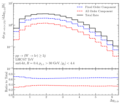
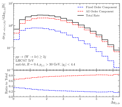
(a)                                                              (b)

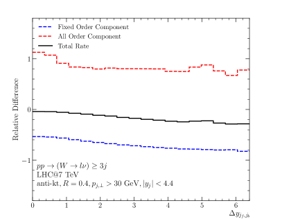
(c)

Figure 12: The differential distribution (black, solid) in the rapidity difference between the most-forward and most-backward jets, $\Delta y_{j_{f},j_{b}}$, in $pp\to(W\to\ell\nu)+\geq 3j$, for (a) case 1, where resummation is applied only to LL states, and (b) case 2, where resummation is applied to all LL and NLL states. Also shown in each case is the breakdown into the component where all-order resummation is applied (red, dashed) and the component which remains described at fixed-order only (blue, dashed). The relative change in each line is shown in (c), using the procedure described in the text.

The first distributions we show (fig. 12) are for the rapidity difference between the most-forward and most-backward jets, $\Delta y_{j_{f},j_{b}}$, for $pp\to(W\to\ell\nu)+\geq 3j$. For case 1 (fig. 12(a)), the all-order component (red, dashed) of the full cross section (black, solid) lies between 30–40% across the range, with the rest coming from fixed-order configurations. There is a dramatic change once resummation is applied also to all NLL states in case 2 (fig. 12(b)), where now the all-order component begins at 65% at $\Delta y_{j_{f},j_{b}}=0$ and rises to 80% by $\Delta y_{j_{f},j_{b}}=6.5$. This immediately illustrates that although the new NLL contributions are formally suppressed, they are numerically highly significant in realistic LHC analyses.

Figure 12(c) shows the relative difference in each of the lines between the two cases. The difference in the total cross section (black line) decreases linearly from close to zero down to $-$25% at large values of $\Delta y_{j_{f},j_{b}}$, while the changes in the components are much larger (between 60% and 110%). The comparatively small change in the total is a sign of the perturbative stability of the HEJ framework. The linear behaviour in each case arises from the relation $y_{j_{f},j_{b}}\sim\log(s_{j_{f},j_{b}}/p_{j_{f},\perp}p_{j_{b},\perp})$ in the MRK limit. Large values of $\Delta y_{j_{f},j_{b}}$ does not guarantee MRK kinematics, but MRK configurations only contribute at the right-hand side of the plot and hence the logarithmic behaviour can still be seen.

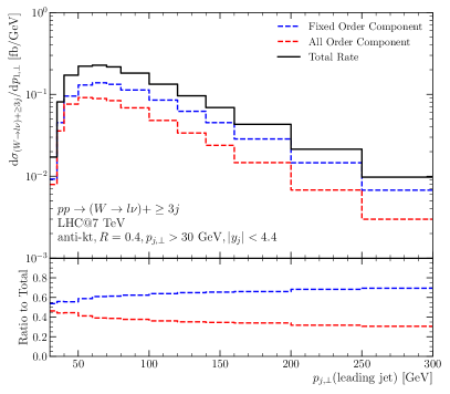
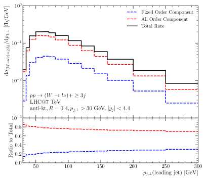
(a)                                                              (b)

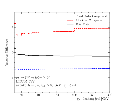
(c)

Figure 13: The differential distribution (black, solid) in the transverse momentum of the leading jet in $pp\to(W\to\ell\nu)+\geq 3j$, without and with resummation applied to NLL states. The panels and lines are as in fig. 12.

In fig. 13, we show the same analysis for the transverse momentum distribution of the leading jet in $pp\to(W\to\ell\nu)+\geq 3j$. Again one can see a dramatic increase in the component of the cross section which is now controlled by all-order resummation, from 30–40% across the range in case 1 (fig. 13(a)) up to 70–80% in case 2 (fig. 13(b)). There is no systematic relation between the high-energy logarithms and transverse momentum and we therefore see that the relative difference in each component is quite flat in this variable. The relative difference in the total cross section is again comparably small at around 8%, while the decrease in the fixed-order component is around $-$30% and the increase in the all-order component is +90–100%.

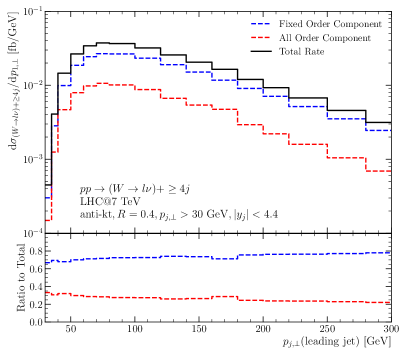
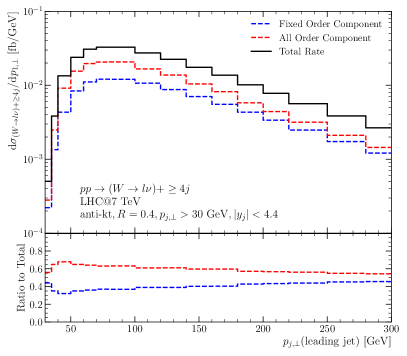
(a)                                                              (b)

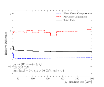
(c)

Figure 14: The differential distribution (black, solid) in the transverse momentum of the leading jet in $pp\to(W\to\ell\nu)+\geq 4j$, without and with resummation applied to NLL states. The panels and lines are as in fig. 12.

In fig. 14, we again show the transverse momentum distribution of the leading jet, but now for $pp\to(W\to\ell\nu)+\geq 4j$. One needs at least four hard jets before the corrections derived in section 3.2 are included. With four jets, there are many more possible final states which are neither LL or NLL, and hence the fraction of the cross-section to which all-order corrections are applied is less here than in fig. 13. However, one can still see the dramatic increase in the all-order component from 20–30% in case 1 (fig. 14(a)) to 55–65% in case 2 (fig. 14(b)). The relative differences seen are very similar to the case of $pp\to(W\to\ell\nu)+\geq 3j$.

In appendix D, we show and discuss more analyses of this kind for exclusive jet rates, the invariant mass distribution of the leading jets and the transverse momentum distribution of the leading jet in $pp\to(W\to\ell\nu)+\geq 2j$.

Having discussed the improvement in the all-order component of HEJ predictions, in the next section we describe a new approach to fixed-order matching such that the fixed-order accuracy of HEJ predictions for $pp\to(W\to\ell\nu)+\geq 2j$ is increased to NLO.

4 All-Order Summation and Kinematic Matching to NLO

The perturbative accuracy obtained in the published predictions so far obtained with HEJ Andersen:2011hs ; Andersen:2012gk ; Andersen:2016vkp ; Andersen:2017kfc ; Andersen:2018tnm ; Andersen:2018kjg is controlled by matching point-by-point to the $n$-jet Born-level matrix element, in this study generated by Sherpa Bothmann:2019yzt with the extension of OpenLoops Buccioni:2017yxi . The $m$-parton, $n$-jet phase space is explored using the efficient procedure described in ref. Andersen:2018tnm , and the $n$-jet samples are merged with the logarithmic accuracy obtained with the resummation. For the study of $W+$jets at hand, fixed-order processes of up to $W+6$-jets are considered, and thus the predictions using the method outlined in Andersen:2018tnm would obtain an accuracy of $\alpha_{s}^{n}$ plus all logarithmic corrections to this of the form $\alpha_{s}^{n}(\alpha_{s}\log(s))^{m}$ and the detailed corrections of the form $\alpha_{s}^{n+1}(\alpha_{s}\log(s))^{m}$, $m>0$, for all observables with contributions from $n=2,\ldots,6$ jets. In this section we will describe a method for extending the fixed-order input to NLO calculations and ensuring that all distributions of $W+n$-jets obtain both full $\alpha_{s}^{n+1}$ (NLO) and all-order logarithmic accuracy.

The matching of logarithmic and fixed next-to-leading order accuracy of distributions is obtained by calculating all distributions of $W+2$-jets at both fixed-order NLO (using again Sherpa Bothmann:2019yzt at fixed order) and for the NLO expansion of the leading and sub-leading logarithmic contributions to the cross section. For the inclusive two-jet rate, HEJ at NLO is obtained by expanding the virtual corrections from the reggeized propagator in the matrix elements for two-parton productions, and truncating the real emissions at a single extra gluon. The organisation of the cancellation of the poles in $\varepsilon$ is performed with the same subtraction method as used in the all-order calculation. Predictions can then be obtained at full NLO and resummed (leading and sub-leading) accuracy of each distribution by the following procedure:

1. obtain histograms for the process at (a) full NLO, (b) HEJ at NLO and (c) full HEJ (including the fixed-order 2-jet and 3-jet subprocesses not subject to resummation which enter (b), but not including these for $\geq 4$-jets).

2. scale each bin in the all-order resummed distribution 1(c) by the ratio of the same bin in the histograms of 1(a) and 1(b).

The final weight in each bin, $w_{\rm HEJ2\,NLO}$, is then given by

$$w_{\rm HEJ2\,NLO}=w_{\rm HEJ2}\frac{w_{\rm NLO}}{w_{\rm HEJ\,at\,NLO}}+w_{\rm FO\,W+\geq 4j},$$ (65)

where $w_{\rm NLO}$ is the weight from full NLO (1(a) above), $w_{\rm HEJ\,at\,NLO}$ is the full HEJ prediction truncated at $\alpha_{s}^{3}$ (1(b) above) and $w_{\rm HEJ2}$ is the inclusive $W+2$-jet prediction from HEJ at all orders plus the 2-jet and 3-jet processes we must add at fixed order (1(c) above). $w_{\rm FO\,W+\geq 4j}$ represents the fixed-order processes at 4-jets and above which do not enter the NLO matching.

In practice, the matching is performed for $W^{+}$ and $W^{-}$ separately, but we find that the matching corrections are similar. A simple expansion of the perturbative series will show that each bin value in the resulting distribution will have full NLO and full logarithmic accuracy. This matching of kinematic distributions to full NLO accuracy corrects distributions in the sub-asymptotic kinematic regions where the leading and sub-leading logarithmic approximation is a poor approximation to the full perturbative result, e.g. high-momentum regions.

We show the matching corrections used in the following section in figs. 15 and 16. Fig. 15 shows the corrections for $W+2$-jet production at 7 TeV for distributions which appear in ref. Aad:2014qxa and fig. 16 shows examples for $W+2$-jet production at 8 TeV for distributions which appear in ref. Aaboud:2017soa . We chose a central scale of $\mu_{r}=\mu_{f}=H_{T}/2$. We varied $\mu_{r}$ and $\mu_{f}$ independently by a factor of two around this central scale choice, keeping their ratio between 0.5 and 2. The scale variation bands are obtained from the envelope of these variations. The jet parameters and cuts are given in the figures. We see that the $p_{j,\perp}$ distributions (figs. 15(a), 15(b), 16(a) and 16(b)) all have a similar shape; they start around 1.5 for low $p_{j,\perp}$ values and then fall until reaching a stable value around 0.7-0.8 for $p_{j,\perp}$ values above about $300$ GeV. A similar drop is also seen in the matching corrections as a function of $p_{W,\perp}$ in fig. 16(c). On the other hand, the impact of matching is independent of the azimuthal separation of the jets, and hence the matching factor in fig. 15(c) is relatively flat. None of the figures show any significant difference between $W^{+}+2j$ production and $W^{-}+2j$ production. The improvement obtained in the description of data from applying these NLO matching corrections will be illustrated in section 5.

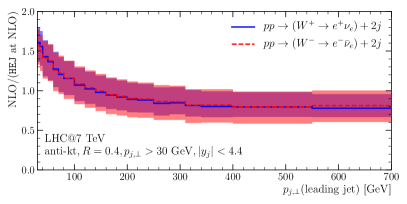
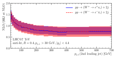
(a)                                                              (b)

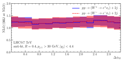
(c)

Figure 15: The NLO matching corrections obtained for the following distributions presented in ref. Aad:2014qxa for inclusive $W^{+}+2j$ production (blue, solid) and $W^{-}+2j$ production (red, dashed): (a) transverse momentum of the leading jet, (b) transverse momentum of the second jet and (c) the difference in azimuthal angle between the leading two jets.

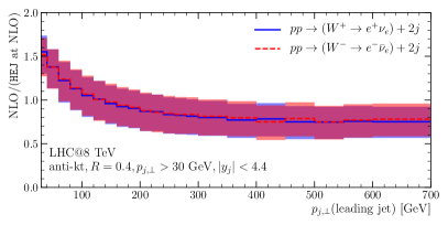
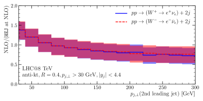
(a)                                                              (b)

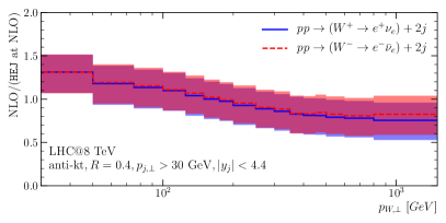
(c)

Figure 16: The NLO matching corrections for the following distributions presented in ref. Aaboud:2017soa for inclusive $W^{+}+2j$ production (blue, solid) and $W^{-}+2j$ production (red, dashed): (a) transverse momentum of the leading jet, (b) transverse momentum of the second jet and (c) the transverse momentum of the $W$ boson.

5 The NLO-matched All-Order Predictions for Measured Quantities

This study has introduced two elements targeted at systematically improving the precision in regions away from asymptotic large energies compared to transverse scales: sub-leading corrections and matching of distributions to next-to-leading order. This section compares predictions to analyses by ATLAS of $W$+dijets at LHC energies of 7 TeV Aad:2014qxa and 8 TeV Aaboud:2017soa , where we focus on distributions where the new components lead to important improvements. The data was collected using slightly different cuts for the electron and muon channel, and then extrapolated to a “combined” selection contrasted with predictions generated with the following cuts listed in table 2. The rapidity selection criteria for jets, accepting jets of rapidities in the full detector, not just the central part, is particularly important for the study of high-energy logarithms: it the same selection criteria as that used for the study of Higgs boson production in association with dijets, and it avoids the focus on jets of very large transverse momenta, which is a result of studying large $m_{jj}$ for solely central jets.

Lepton $p_{\textrm{T}}$	$p_{\textrm{T}}$$>25$ GeV
Lepton rapidity	$|\eta|<2.5$
Missing transverse momentum	$E^{\textrm{miss}}_{\textrm{T}}>25$ GeV
Reconstructed transverse mass of boson	$m_{\textrm{T}}>40$ GeV
Jet $p_{\textrm{T}}$	$p_{\textrm{T}}>30$ GeV
Jet rapidity	$|y|<4.4$
Jet isolation	$\Delta R(l,\textrm{jet})>0.5$ (7 TeV Aad:2014qxa ), 0.4 (8 TeV Aaboud:2017soa )
	jet is removed

Table 2: The selection cuts used for the comparisons to data.

We will compare the measured data with the fixed-order predictions for $W$+dijets at NLO obtained using Sherpa Bothmann:2019yzt with the extension of OpenLoops Buccioni:2017yxi and those of HEJ obtained using the improvements presented in the present paper. We use the NNPDF3.1nlo pdf set Ball:2017nwa as provided by LHAPDF6 Buckley:2014ana . In particular we will compare the predictions for the inclusive and exclusive jet counts, the transverse momenta of the leading and sub-leading jet and of the $W$-boson, and the azimuthal angle between the two leading jets. A central scale of $\mu_{f}=\mu_{r}=H_{T}/2$ is chosen for all predictions, and the scale variation band are the envelope of an independent variation of each scale by up to a factor up 2, except configurations with a ratio between them larger than 2 (or smaller than $1/2$). This scale choice is guided purely by the convention for fixed-order predictions — it has not been tuned in order to obtain a good fit of data to the predictions of HEJ.

The impact on observables of including resummation of the next-to-leading processes and the NLO matching have been shown separately in section 3 and section 4 respectively. In this section, we show the new predictions combining both improvements (labelled “HEJ2 NLO”, shown in green). We also show the previously available predictions based on just the leading logarithmic description Andersen:2012gk combined with matching to high-multiplicity Born-level matrix elements (labelled “HEJ1”, shown in blue). The HEJ1 predictions failed systematically in the regions of large ($>100$GeV) transverse momenta of the jets — this specifically breaks the multi-Regge kinematic conditions that the leading logarithmic approximation is based upon. This feature showcases one of the shortcomings of the matching of the non-resummable part of the cross section by a naïve addition of Born-level events of increasing multiplicity: these Born-level predictions should be considered inclusive in the jet multiplicity, so simply adding the contribution from the samples leads to overestimated cross sections – just as found. While this question, related to the higher-order perturbative corrections to each sample, is not solved by including the sub-leading corrections, the contribution from the non-resummable part of the cross section at large transverse momenta is reduced from 60% when resumming only the processes contributing at leading-logarithmic accuracy to less than 35% when the next-to-leading subprocesses are included in the all-order treatment (figure 23). The reduction in the contribution from fixed-order events obviously reduces the impact of their slight perturbative mis-use.

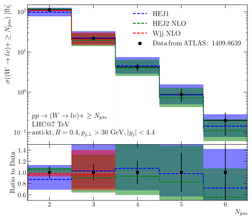
(a) Inclusive jet rates.

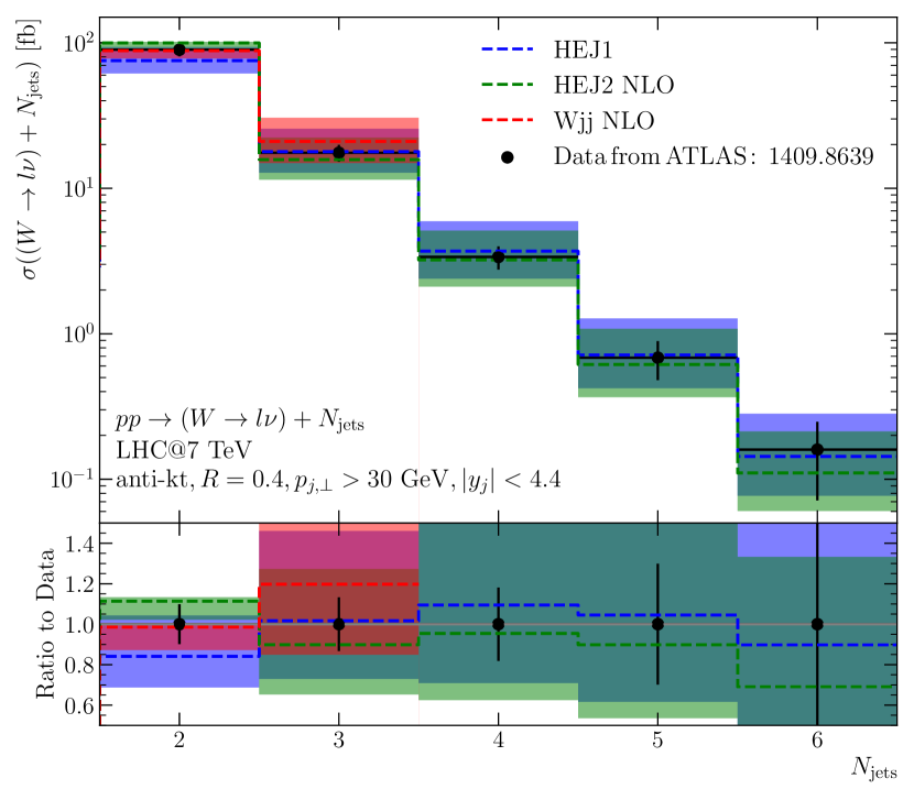
(b) Exclusive jet rates.

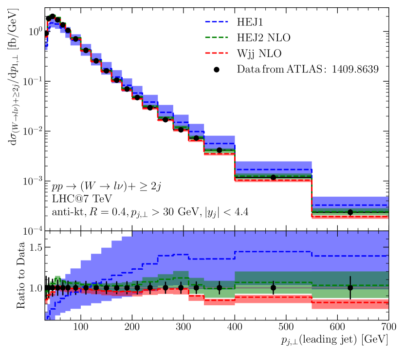
(c) Differential cross section for the transverse momentum of the leading jet.

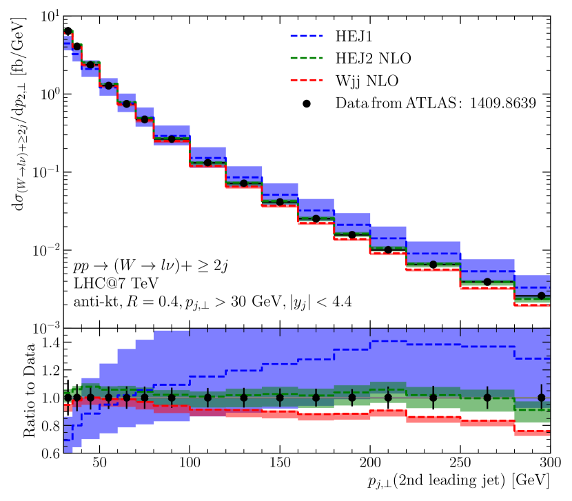
(d) Differential cross section for the transverse momentum of the second leading jet.

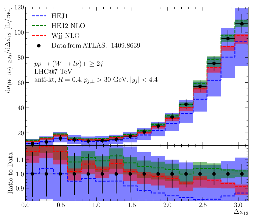
(e) Differential cross section for the azimuthal angle between the two leading jets.

Figure 17: Predictions for $pp\to(W\to l\nu)+\geq 2j$ for LHC@7TeV, compared to ATLAS data from Aad:2014qxa . The original HEJ1 predictions are shown in blue, the pure NLO predictions are shown in red and the new HEJ2 predictions incorporating the methods of sections 3 and 4 are shown in green.

Figs. 17(a)-17(b) compare the predictions for the inclusive and exclusive jet rates respectively to data. The inclusive 2-jet rate is matched to NLO accuracy, which as expected decreases the scale dependence compared to the predictions obtained with HEJ1 reported in Aad:2014qxa . The central predictions for both the inclusive and exclusive rates now agree more closely with the data. The scale variation of the 2-jet bin is significantly reduced due to the NLO matching in that bin. It is worth noting that while the scale variation in the inclusive 2-jet bin from pure NLO is smaller than that of the NLO-matched HEJ 2, the scale variation in the exclusive 2-jet bin of fig. 17(b) are similar for the NLO-calculation and the NLO-matched HEJ2.

Figs. 17(c)-17(d) demonstrates, as expected, that the impact of including the sub-leading processes in the resummation is significant for the description of scatterings at large transverse momenta. Indeed, all the problems identified with the description in HEJ1 are solved in HEJ2. The description of the spectrum of the leading and sub-leading jet is better still than that of pure $W+$dijets at NLO. The scale variation is slightly larger which is due to the corrections at $\alpha_{s}^{4}$ and above included in the HEJ2 predictions.

Finally, fig. 17(e) shows the differential distribution for the azimuthal angle between the two hardest jets, $\phi_{12}$. Again, the already decent description of HEJ1 is slightly improved in HEJ2, and the scale variation is reduced. Overall, the agreement with data for this observable is similar to that reached at pure NLO.

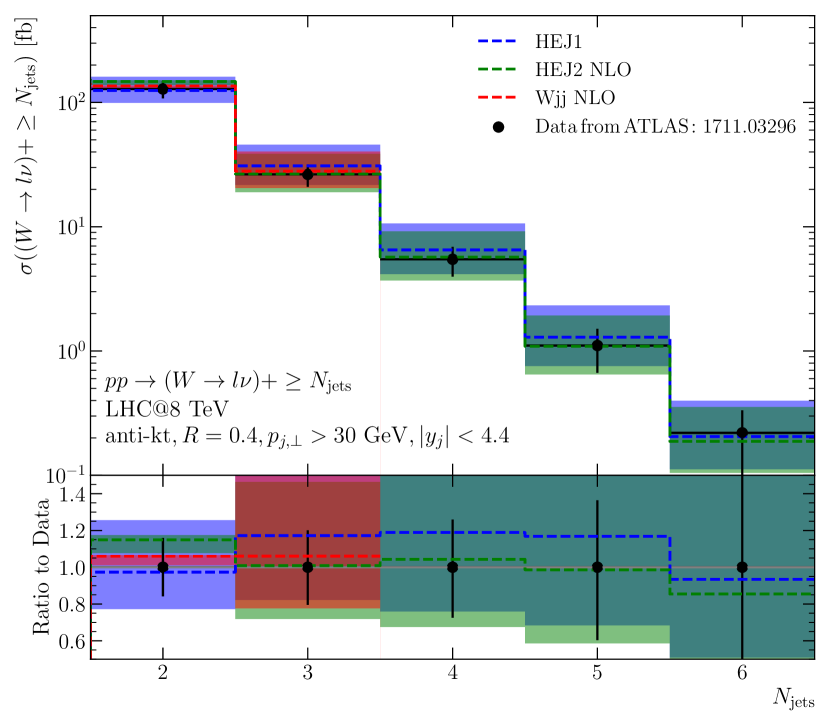
(a) Inclusive jet rates.

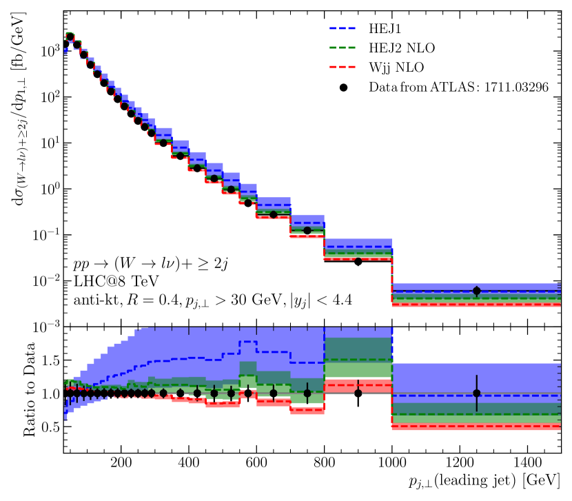
(b) Differential cross section for the transverse momentum of the leading jet.

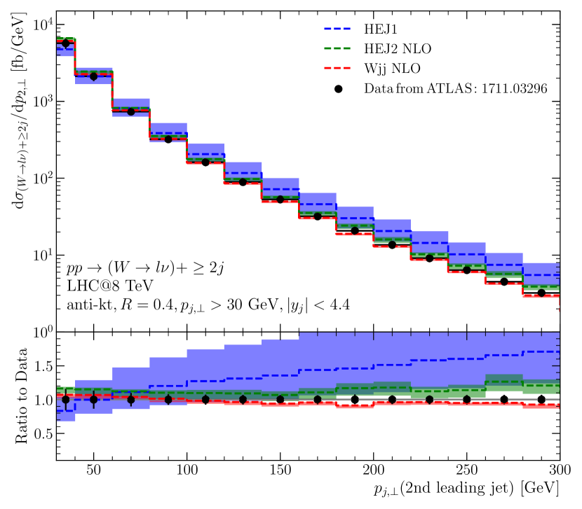
(c) Differential cross section for the transverse momentum of the second leading jet.

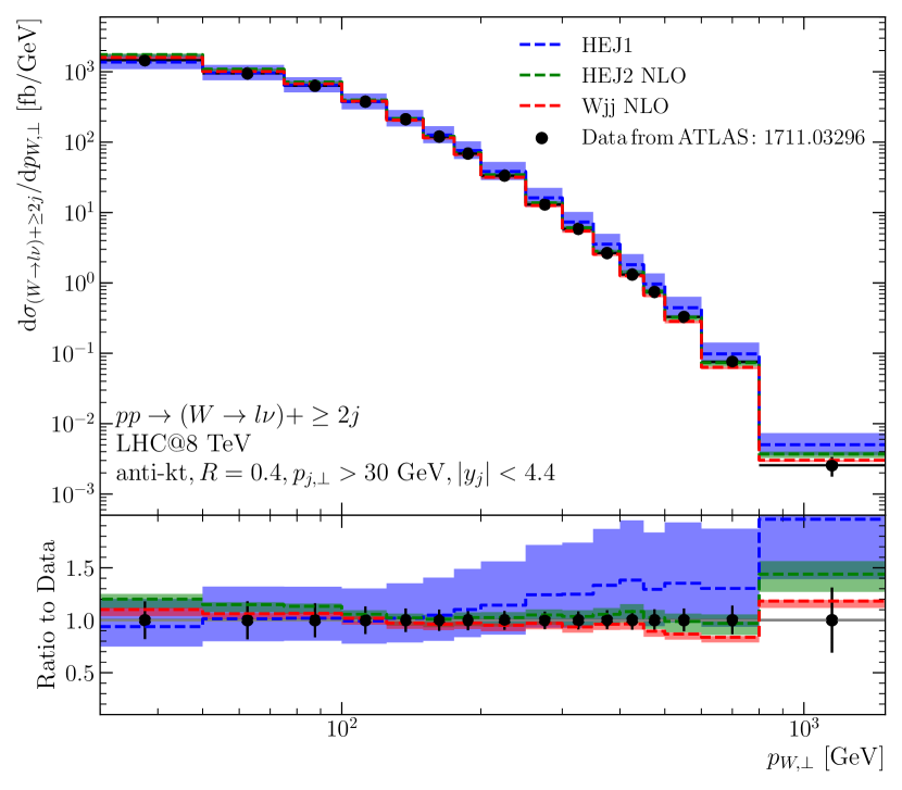
(d) Differential cross section for the transverse momentum of the boson.

Figure 18: Predictions for $pp\to(W\to l\nu)+\geq 2j$ for LHC@8TeV, compared to ATLAS data from Aaboud:2017soa . The original HEJ1 predictions are shown in blue, the pure NLO predictions are shown in red and the new HEJ2 predictions incorporating the methods of sections 3 and 4 are shown in green.

The comparison to the relevant results from the updated analysis for 8 TeV collisions and similar cuts is presented in fig. 18. Of course very little changes in the calculations, and the conclusions are similar to those arrived at for the 7 TeV analysis. The inclusive rates arrived at with HEJ2 show an extremely good agreement with data across all the matched multiplicities 2–6 inclusive. The transverse momentum is described extremely well for data available for the first and second hardest jet, and for the $W$-boson.

The comparison with data clearly demonstrates that the combined effect of matching to $W+$dijets at NLO and the inclusion of sub-leading channels in the all-order treatment has repaired the short-comings of the previous approach based solely on Born level matching and leading-logarithmic resummation. The scale variation is reduced in line with the NLO input, and the distributions associated with sub-leading regions of phase space, such as large transverse momenta, are now described well.

6 Conclusions

The High Energy Jets (HEJ) framework provides a description of collider events with at least two jets, which combines fixed-order accuracy with leading-logarithmic accuracy in $\hat{s}/p_{t}^{2}$. These logs dominate in the MRK limit and have been shown to be important in describing data at large invariant mass or large rapidity separation of jets. However, the description consistently struggled to give a good description of data in other regions of phase space which are not directly related to the high energy limit, regions with large transverse momentum for example. In this paper, we have directly addressed this by focussing on $pp\to(W\to\ell\nu)+\geq 2j$ and increasing the perturbative accuracy of the HEJ2 predictions in a two-pronged approach:

1. In section 3, we calculated the components needed to include logarithmic corrections to all of the partonic channels contributing to the first sub-leading corrections at high energies for the process $pp\to W+\geq 2j$. While this forms a well-defined contribution at NLL to the inclusive $W+2j$ cross section, it is only a part of the full NLL correction. We showed in section 3.3 that the included processes led to a significant increase in the fraction of the cross section which is supplemented with all-order corrections, for example up to at least 75% across all values of $p_{j,\perp}$ for the leading jet in $pp\to(W\to\ell\nu)+\geq 3j$ compared to 35% without the new corrections (fig. 13). Most impressively, the change in the perturbative treatment of such a large part of the cross section leads to only very modest changes of a few percent. This behaviour is a testament to the stability introduced to the perturbative series by including the logarithmic corrections.

2. In section 4, we presented a new method of fixed-order matching which leads to next-to-leading order accuracy for the measured distributions, while keeping the same logarithmic accuracy. The matching factors shown in figs. 15 and 16 can be seen, for example, to slightly suppress the all-order predictions for values of transverse momentum above $\sim 100$ GeV.

The new predictions from HEJ2, combining the two new components above, are compared to LHC data in section 5. We have shown in figs. 17 and 18 that the new predictions deliver an excellent description of all the measured quantities in sub-leading regions of phase space. They dramatically improve upon the original predictions from HEJ1 in all distributions. Furthermore, in many cases they also provide a better prediction than that obtained from pure NLO, showing that HEJ2 combines the best of both fixed-order and leading-logarithmic descriptions.

The QCD radiation pattern arising from colour-octet exchange is known to be very similar across QCD inclusive dijet production, $W+\geq 2j$, $Z+\geq 2j$ and $H+\geq 2j$. Hence the perturbative approach developed in this paper offers an exciting new tool to describe a large range of key processes at the LHC.

Appendix A Phase Space Slices

Here we give the parameters of the phase space slices used in the explorer plots in section 3. We begin with fig. 9, where the outgoing momenta are given by:

$$\begin{split}p_{i}&=(k_{\perp i}\cosh(y_{i}),k_{\perp i}\cos(\phi_{i}),k_{\perp i}\sin(\phi_{i}),k_{\perp i}\sinh(y_{i})),\\ k_{\perp 1}&=k_{\perp 2}=k_{\perp\bar{\ell}}=40~{}\mathrm{GeV},\ k_{\perp\ell}=\frac{m_{V}^{2}}{2k_{\perp\bar{\ell}}(\cosh(y_{\bar{\ell}}-y_{\ell})-\cos(\phi_{\bar{\ell}}-\phi_{\ell}))},\\ \phi_{1}&=2\pi/3,\ \phi_{2}=0,\ \phi_{\bar{\ell}}=\pi/2,\ \phi_{\ell}=-\pi/2,\\ y_{1}&=\Delta,\ y_{2}=0,\ y_{3}=-\Delta,\ y_{\bar{\ell}}=\Delta,\ y_{\ell}=\Delta,\\ p_{3\perp}&=-p_{1\perp}-p_{2\perp}-p_{\bar{\ell}\perp}-p_{\ell\perp}.\end{split}$$ (66)

In fig. 11, the phase space slice used is

$$\begin{split}p_{i}&=(k_{\perp i}\cosh(y_{i}),k_{\perp i}\cos(\phi_{i}),k_{\perp i}\sin(\phi_{i}),k_{\perp i}\sinh(y_{i})),\\ k_{\perp 1}&=k_{\perp 2}=k_{\perp 3}=k_{\perp\bar{\ell}}=40~{}\mathrm{GeV},\ k_{\perp\ell}=\frac{m_{V}^{2}}{2k_{\perp\bar{\ell}}(\cosh(y_{\bar{\ell}}-y_{\ell})-\cos(\phi_{\bar{\ell}}-\phi_{\ell}))},\\ \phi_{1}&=\pi,\ \phi_{2}=\pi/2,\ \phi_{3}=-\pi/3,\ \phi_{\bar{\ell}}=\pi/4,\ \phi_{\ell}=-\pi/4,\\ y_{1}&=\Delta,\ y_{2}=\Delta/3,\ y_{3}=-\Delta/3,\ y_{4}=-\Delta,\ y_{\bar{\ell}}=-\Delta/3,\ y_{\ell}=-\Delta/3,\\ p_{4\perp}&=-p_{1\perp}-p_{2\perp}-p_{3\perp}-p_{\bar{\ell}\perp}-p_{\ell\perp}.\end{split}$$ (67)

These are provided in order to allow the results to be reproduced, but we stress that the level of agreement does not depend on the specific choices of these points.

Appendix B Derivation of New NLL Components in $W+3$-jet Processes

B.1 Emission of an Unordered Gluon and a $W$ Boson from the Same Quark Line

Here we derive the current, $j_{W{\rm uno}\,\mu}^{d}(p_{a},p_{1},p_{2},p_{\ell},p_{\bar{\ell}})$, given in eq. 28 in the main text. We do this by considering the process given in eq. 25, defined such that the $W$ boson may only be emitted from the $p_{a}$–$p_{2}$ quark line. We assume that the rapidities of the final-state partons obey $y_{1}\sim y_{2}\ll y_{3}$; we make no assumption for the $W$ boson or its decay products. We are aiming to write the amplitude in the form given in eq. 27.

There are 12 Feynman diagrams in total at leading-order. We split these by colour structure into four categories and give one example of each in fig. 19.

(a)

(b)

(c)

(d)

Figure 19: Examples of each of the four categories of Feynman diagram which contribute at leading-order: (a) where the gluon and $W$ boson are emitted from the same quark line and the gluon comes after the $t$-channel propagator, (b) where the gluon and $W$ boson are emitted from the same quark line and the gluon comes before the $t$-channel proagator, (c) the gluon is emitted from the $t$-channel gluon and in (d) the gluon is emitted from the $b$–$3$ quark line.

We begin with diagrams where the $W$ boson and unordered gluon are emitted from the same quark line, with the gluon emitted after the $t$-channel as in the example in fig. 19(a). The sum of the 3 diagrams of this kind gives (using $u_{i}$ as shorthand for $u^{h_{i}}(p_{i})$, $s_{ij}=(p_{i}+p_{j})^{2}$, $s_{ijk}=(p_{i}+p_{j}+p_{k})^{2}$ and $t_{ij}=(p_{i}-p_{j})^{2}$)

$$A=-g_{s}^{3}T^{d}_{3b}\frac{\left[\bar{u}_{3}\gamma_{\mu}u_{b}\right]}{t_{b3}}\cdot\varepsilon_{\nu}(p_{1})\ \left[\bar{u}_{\ell}\gamma_{\rho}v_{\bar{\ell}}\right]\cdot\left(iT^{1}_{2i}T^{d}_{ia}\tilde{U}_{1}^{\nu\mu\rho}\right),$$ (68)

where

$$\begin{split}\tilde{U}_{1}^{\nu\mu\rho}=&K_{W}\bigg{(}\frac{[\bar{u}_{2}\gamma^{\nu}(\not{p}_{2}+\not{p}_{1})\gamma^{\mu}(\not{p}_{a}-\not{p}_{W})\gamma^{\rho}u_{a}]}{s_{12}t_{aW}}+\frac{[\bar{u}_{2}\gamma^{\nu}(\not{p}_{2}+\not{p}_{1})\gamma^{\rho}(\not{p}_{2}+\not{p}_{1}+\not{p}_{W})\gamma^{\mu}u_{a}]}{s_{12}s_{12W}}\\ &+\frac{[\bar{u}_{2}\gamma^{\rho}(\not{p}_{2}+\not{p}_{W})\gamma^{\nu}(\not{p}_{1}+\not{p}_{2}+\not{p}_{W})\gamma^{\mu}u_{a}]}{s_{2W}s_{12W}}\bigg{)},\end{split}$$ (69)

and we have introduced the factor

$$K_{W}=\left(\frac{ig_{W}}{\sqrt{2}}\right)^{2}\frac{1}{\left(p_{W}^{2}-m_{W}^{2}+im_{W}\Gamma_{W}\right)}.$$ (70)

These diagrams already have the colour and kinematic structure of eq. 27 and therefore no further approximation is applied.

The next category of Feynman diagrams is where the $W$ and gluon are emitted from the same quark line, but now the gluon is emitted before the $t$-channel gluon. An example is shown in fig. 19(b). This is very similar to the first kind and the sum of the three diagrams in this category is given by

$$B=-g_{s}^{3}T^{d}_{3b}\frac{[\bar{u}_{3}\gamma_{\mu}u_{b}]}{t_{b3}}\cdot\varepsilon_{\nu}(p_{1})\ [\bar{u}_{\ell}\gamma_{\rho}v_{\bar{\ell}}]\cdot\left(iT^{d}_{2i}T^{1}_{ia}\tilde{U}_{2}^{\nu\mu\rho}\right),$$ (71)

where

$$\begin{split}\tilde{U}_{2}^{\nu\mu\rho}=&K_{W}\bigg{(}\frac{[\bar{u}_{2}\gamma^{\mu}(\not{p}_{a}-\not{p}_{W}-\not{p}_{1})\gamma^{\nu}(\not{p}_{a}-\not{p}_{W})\gamma^{\rho}u_{a}]}{t_{aW1}t_{aW}}+\frac{[\bar{u}_{2}\gamma^{\mu}(\not{p}_{a}-\not{p}_{W}-\not{p}_{1})\gamma^{\rho}(\not{p}_{a}-\not{p}_{1})\gamma^{\nu}u_{a}]}{t_{a1W}t_{a1}}\\ &+\frac{[\bar{u}_{2}\gamma^{\rho}(\not{p}_{2}+\not{p}_{W})\gamma^{\mu}(\not{p}_{a}-\not{p}_{1})\gamma^{\nu}u_{a}]}{s_{2W}t_{a1}}\bigg{)}.\end{split}$$ (72)

Here we have used the further shorthand notation $t_{ijk}=(t_{i}-t_{j}-t_{k})^{2}$. These diagrams also already have the structure shown in eq. 27 and hence no further approximation is made.

The next category of Feynman diagrams we will consider are the two where the outgoing gluon is emitted from the $t$-channel gluon propagator, e.g. fig. 19(c). The sum of the two gives

$$\begin{split}C=&\ g_{s}^{3}K_{W}T^{d}_{3b}\frac{[\bar{u}_{3}\gamma_{\mu}u_{b}]}{t_{b3}}\cdot\varepsilon_{\nu}(p_{1})\ [\bar{u}_{\ell}\gamma_{\rho}v_{\bar{\ell}}]\cdot f^{ed1}T^{e}_{2a}\\ &\times\frac{1}{t_{aW2}}\left(\frac{[\bar{u}_{2}\gamma^{\sigma}(\not{p}_{a}-\not{p}_{W})\gamma^{\rho}u_{a}]}{t_{aW}}+\frac{[\bar{u}_{2}\gamma^{\rho}(\not{p}_{2}+\not{p}_{W})\gamma^{\sigma}u_{a}]}{s_{2W}}\right)\\ &\times\left(g^{\sigma\mu}(q_{1}+q_{2})^{\nu}+g^{\mu\nu}(-q_{2}+p_{1})^{\sigma}-g^{\nu\sigma}(p_{1}+q_{1})^{\mu}\right),\end{split}$$ (73)

where $q_{1}$, $q_{2}$ are the $t$-channel momenta flowing into and out of the 3-gluon vertex: $q_{1}=p_{a}-p_{2}-p_{W}$ and $q_{2}=q_{1}-p_{1}$. These diagrams also immediately satisfy the structure of eq. 27. There is some freedom in how one writes the expression in the last term of eq. 73 in $W+3j$, because any term proportional to $q_{2}^{\mu}$ gives zero. We will take $-(p_{1}+q_{1})^{\mu}=-2p_{1}^{\mu}-q_{2}^{\mu}$ and remove the zero-contribution from $q_{2}^{\mu}$. This is the unique choice which remains gauge invariant when we generalise our current to processes with an arbitrary number of extra emissions.

Finally we consider the diagrams in which the gluon and $W$ are emitted from different quark lines, as in the example in fig. 19(d). The full expression for that diagram is given by

$$\begin{split}D_{\rm(d)}&=\ -ig_{s}^{3}K_{W}T^{d}_{2a}T^{1}_{3i}T^{d}_{ib}\ \ \varepsilon_{\nu}(p_{1})\ [\bar{u}_{\ell}\gamma_{\rho}v_{\bar{\ell}}]\\ &\ \times\left(\frac{[\bar{u}_{2}\gamma^{\mu}(\not{p}_{a}-\not{p}_{W})\gamma^{\rho}u_{a}]\ [\bar{u}_{3}\gamma^{\nu}(\not{p}_{1}+\not{p}_{3})\gamma_{\mu}u_{b}]}{t_{aW}s_{13}t_{b13}}\right).\end{split}$$ (74)

This is our first example which does not satisfy the structure of eq. 27 and so we need to make some approximation. In the high energy limit, $p_{b}$ and $p_{3}$ are dominated by their forward lightcone components, while $p_{a}$, $p_{1}$ and $p_{2}$ are dominated by their backward lightcone components. This automatically means that e.g. $s_{a1}\ll s_{a3}$. By considering the contractions of the $\mu$-index, and of the $\nu$-index for a generic reference vector in $\varepsilon_{\nu}(p_{1})$, in this limit the $\not{p}_{1}$-term is suppressed compared to the $\not{p}_{3}$-term in the second spinor term by ratios of invariants like $s_{a1}/s_{a3}$. We therefore drop this term and find

$$\begin{split}D_{\rm(d)}\approx&\ -ig_{s}^{3}K_{W}T^{d}_{2a}T^{1}_{3i}T^{d}_{ib}\ \varepsilon_{\nu}(p_{1})\ [\bar{u}_{\ell}\gamma_{\rho}v_{\bar{\ell}}]\\ &\ \times\left(\frac{[\bar{u}_{2}\gamma^{\mu}(\not{p}_{a}-\not{p}_{W})\gamma^{\rho}u_{a}]\ [\bar{u}_{3}\gamma_{\mu}u_{b}]\ 2p_{3}^{\nu}}{t_{aW}s_{13}t_{b13}}\right).\end{split}$$ (75)

We perform the same approximation for the other 3 diagrams in this category, to get the sum of the four to be

$$\begin{split}D\approx&\ -ig_{s}^{3}K_{W}\varepsilon_{\nu}(p_{1})\ [\bar{u}_{\ell}\gamma_{\rho}v_{\bar{\ell}}]\ \frac{[\bar{u}_{3}\gamma_{\mu}u_{b}]}{t_{b13}}\left(T^{d}_{2a}T^{d}_{3i}T^{1}_{ib}\frac{2p_{b}^{\nu}}{t_{b1}}+T^{d}_{2a}T^{1}_{3i}T^{d}_{ib}\frac{2p_{3}^{\nu}}{s_{13}}\right)\\ &\ \times\left(\frac{[\bar{u}_{2}\gamma^{\mu}(\not{p}_{a}-\not{p}_{W})\gamma^{\rho}u_{a}]}{t_{aW}}+\frac{[\bar{u}_{2}\gamma^{\rho}(\not{p}_{2}+\not{p}_{W})\gamma^{\mu}u_{a}]}{s_{2W}}\right).\end{split}$$ (76)

In the QMRK, $p_{3}$ is dominated by its positive lightcone component, taken to be roughly equal to $p_{b}$: $p_{3}\sim p_{b}=p_{+}$. We use this approximation to combine the colour factor:

$$\begin{split}D\approx&\ -ig_{s}^{3}K_{W}\varepsilon_{\nu}(p_{1})\ [\bar{u}_{\ell}\gamma_{\rho}v_{\bar{\ell}}]\ \frac{[\bar{u}_{3}\gamma_{\mu}u_{b}]}{t_{b13}}\left(iT^{d}_{2a}f^{1de}T^{e}_{3b}\ \frac{2p_{+}^{\nu}}{s_{1+}}\right)\\ &\ \times\left(\frac{[\bar{u}_{2}\gamma^{\mu}(\not{p}_{a}-\not{p}_{W})\gamma^{\rho}u_{a}]}{t_{aW}}+\frac{[\bar{u}_{2}\gamma^{\rho}(\not{p}_{2}+\not{p}_{W})\gamma^{\mu}u_{a}]}{s_{2W}}\right).\end{split}$$ (77)

We can now choose to symmetrise the $p_{+}$-term to reinstate the original symmetry of the process. Our final expression for the sum of these diagrams is therefore

$$\begin{split}D\approx&\ g_{s}^{3}K_{W}\varepsilon_{\nu}(p_{1})\ [\bar{u}_{\ell}\gamma_{\rho}v_{\bar{\ell}}]\ \frac{[\bar{u}_{3}\gamma_{\mu}u_{b}]}{t_{b13}}\cdot T^{e}_{2a}f^{1ed}T^{d}_{3b}\cdot\frac{1}{2}\left(\frac{p_{b}^{\nu}}{p_{b}.p_{1}}+\frac{p_{3}^{\nu}}{p_{1}.p_{3}}\right)\\ &\ \times\left(\frac{[\bar{u}_{2}\gamma^{\mu}(\not{p}_{a}-\not{p}_{W})\gamma^{\rho}u_{a}]}{t_{aW}}+\frac{[\bar{u}_{2}\gamma^{\rho}(\not{p}_{2}+\not{p}_{W})\gamma^{\mu}u_{a}]}{s_{2W}}\right).\end{split}$$ (78)

We notice that this has an identical factor to the third category of Feynman diagram and we therefore write their sum as

$$C+D\approx\ g_{s}^{3}T^{d}_{3b}\frac{[\bar{u}_{3}\gamma_{\mu}u_{b}]}{t_{b3}}\varepsilon_{\nu}(p_{1})\ [\bar{u}_{\ell}\gamma_{\rho}v_{\bar{\ell}}]\left(f^{1de}T^{e}_{2a}\tilde{L}^{\nu\mu\rho}\right)$$ (79)

where

$$\tilde{L}^{\nu\mu\rho} =\frac{K_{W}}{t_{aW2}}\left(\frac{[\bar{u}_{2}\gamma_{\sigma}(\not{p}_{a}-\not{p}_{W})\gamma^{\rho}u_{a}]}{t_{aW}}+\frac{[\bar{u}_{2}\gamma^{\rho}(\not{p}_{2}+\not{p}_{W})\gamma_{\sigma}u_{a}]}{s_{2W}}\right)$$ (80)

$$\vphantom{+\frac{1}{t_{aW2}}}\quad\times\left(\left(\frac{p_{b}^{\nu}}{s_{1b}}+\frac{p_{3}^{\nu}}{s_{13}}\right)(q_{1}-p_{1})^{2}g^{\sigma\mu}+g^{\sigma\mu}(2q_{1}-p_{1})^{\nu}+g^{\mu\nu}(2p_{1}-q_{1})^{\sigma}-2g^{\nu\sigma}p_{1}^{\mu}\right).$$

The presence of $p_{b}$ and $p_{3}$ in this equation at first looks like it spoils the factorised structure we were looking for. However, dependence on outer partons mirrors our Lipatov vertex description of extra emissions: the traditional form would contain projection operators for lightcone components, where we choose to restore some of the underlying physics by using the average of a contraction with $p_{b}$ and $p_{3}$ instead Andersen:2009nu . The choice will only affect sub-leading terms. The critical point is that we do not have dependence on any other emission, so the complexity does not increase with the number of final state particles.

We can now deduce the current we need, $j^{\mu}_{\rm Wuno}(p_{a},p_{1},p_{2},p_{\ell},p_{\bar{\ell}})$, by comparing the sum of eqs. 68, 71 and 79 to eq. 27. We find

$$\begin{split}j^{\mu}_{\rm Wuno}(p_{a},p_{1},p_{2},p_{\ell},p_{\bar{\ell}})=&\ -i\varepsilon_{\nu}(p_{1})\ [\bar{u}_{\ell}\gamma_{\rho}v_{\bar{\ell}}]\\ &\ \times\left(T^{1}_{2i}T^{d}_{ia}(\tilde{U}_{1}^{\nu\mu\rho}-\tilde{L}^{\nu\mu\rho})+T^{d}_{2i}T^{1}_{ia}(\tilde{U}_{2}^{\nu\mu\rho}+\tilde{L}^{\nu\mu\rho})\right),\end{split}$$ (81)

where the tensors $\tilde{U}_{1}^{\nu\mu\rho}$, $\tilde{U}_{2}^{\nu\mu\rho}$ and $\tilde{L}^{\nu\mu\rho}$ are given in eqs. 69, 72 and 80. Later in section 3.1, in eq. 34, these tensors are used in processes with $n-3$ additional gluon emissions. In this case, $p_{3}$ should be mapped to $p_{n}$.

B.2 Emission of an Unordered Gluon from a Quark Line

Here we give $j^{d,h_{b},h_{2},h_{3}\,\mu}_{\rm uno}(p_{b},p_{2},p_{3})$, originally derived in Andersen:2017kfc , and used in this paper in eq. 36 to describe an unordered gluon emission from an incoming-outgoing quark line in processes where the $W$ boson is emitted from a different quark line:

$$j^{d,h_{b},h_{2},h_{3}\,\mu}_{\rm uno}(p_{b},p_{2},p_{3})=-i\varepsilon_{\nu}(p_{3})\left(T^{3}_{2i}T^{d}_{ib}\left(U_{1}^{\mu\nu}-L^{\mu\nu}\right)+T^{d}_{2i}T^{3}_{ib}\left(U_{2}^{\mu\nu}+L^{\mu\nu}\right)\right),$$ (82)

with

$$\begin{split}U_{1}^{\mu\nu}&=\frac{1}{s_{23}}\left([\bar{u}_{2}^{h_{2}}\gamma^{\nu}u^{h_{2}}_{3}][\bar{u}_{3}^{h_{b}}\gamma^{\mu}u^{h_{b}}_{b}]+2p_{2}^{\nu}[\bar{u}_{2}^{h_{b}}\gamma^{\mu}u_{b}^{h_{b}}]\right),\\ U_{2}^{\mu\nu}&=\frac{1}{t_{b3}}\left(2p_{b}^{\nu}[\bar{u}^{h_{2}}_{2}\gamma^{\mu}u^{h_{2}}_{b}]-[\bar{u}_{2}^{h_{2}}\gamma^{\mu}u^{h_{2}}_{3}][\bar{u}^{h_{b}}_{3}\gamma^{\nu}u^{h_{b}}_{b}]\right),\\ L^{\mu\nu}&=\frac{1}{t_{b2}}\left(-2p^{\mu}_{3}[\bar{u}_{2}^{h_{b}}\gamma^{\nu}u^{h_{b}}_{b}]+2p_{3}^{\rho}[\bar{u}_{2}^{h_{b}}\gamma_{\rho}u^{h_{b}}_{b}]g^{\mu\nu}\vphantom{\frac{p_{a}^{\nu}}{t_{a3}}}\right.\\ &\qquad\quad\left.+(q_{2}+q_{3})^{\nu}[\bar{u}_{2}^{h_{b}}\gamma^{\mu}u^{h_{b}}_{b}]+q_{2}^{2}[\bar{u}_{2}^{h_{b}}\gamma^{\mu}u^{h_{b}}_{b}]\left(\frac{p_{1}^{\nu}}{s_{13}}-\frac{p_{a}^{\nu}}{t_{a3}}\right)\right),\end{split}$$ (83)

where the derived $t$-channel momenta here are $q_{2}=p_{b}-p_{2}-p_{3}$ and $q_{3}=p_{b}-p_{2}$. The separate spinor strings in $U_{1}$ and $U_{2}$ arise from splitting a longer spinor string using completeness relations which means that the helicities do not always match the helicity of the corresponding particle. Note these expressions are zero unless $h_{b}=h_{2}$.

In order to generalise this expression to events with $n-3$ additional gluon emissions, one should make the replacements $p_{2}\to p_{n-1}$ and $p_{3}\to p_{n}$, where the numbering runs over all outgoing coloured particles in increasing order of rapidity.

Appendix C Derivation of New NLL Components in $W+4$-jet Processes

C.1 Emission of a Central $Q\bar{Q}$ Pair

In this section, we outline the derivation of the tensor $X_{\rm cen}^{de\,\mu\nu}$, which is introduced in eq. 54 in the main text to describe processes with a $Q\bar{Q}$ emission between the most forward and backward partons, e.g. fig. 10(a). We derive the necessary component by considering $q\tilde{q}\to qQ\bar{Q}\tilde{q}$, eq. 51. There are seven Feynman diagrams at leading-order, shown in fig. 20. We define $t_{i}=q_{i}^{2}$ where $q_{i}$ are defined as in section 3, which in this context is $q_{1}=p_{a}-p_{1}$ and $q_{3}=p_{4}-p_{b}$. We choose not to use $q_{2}$ here as it would depend on the rapidity ordering of $Q$ and $\bar{Q}$ which we do not specify.

Figure 20: All Feynman diagrams which contribute to $q\tilde{q}\to qQ\bar{Q}\tilde{q}$ at leading order.

The first diagram is given by

$$iA_{1}=\frac{-ig_{s}^{4}T^{e}_{1i}T^{g}_{ia}T^{e}_{23}T^{g}_{4b}}{s_{23}t_{3}}\left[\bar{u}_{1}\gamma^{\mu}\frac{(\not{p}_{1}+\not{p}_{2}+\not{p}_{3})}{(p_{1}+p_{2}+p_{3})^{2}}\gamma^{\rho}u_{a}\right]\left[\bar{u}_{2}\gamma_{\mu}v_{3}\right]\left[\bar{u}_{4}\gamma_{\rho}u_{b}\right].$$ (84)

As in section B.1, we will expand the square bracket using completeness relations:

$$\frac{1}{s_{12}+s_{13}+s_{23}}\left(2p_{1}^{\mu}\left[\bar{u}_{1}\gamma^{\rho}u_{a}\right]+\left[\bar{u}_{1}\gamma^{\mu}u_{2}\right]\left[\bar{u}_{2}\gamma^{\rho}u_{a}\right]+\left[\bar{u}_{1}\gamma^{\mu}u_{3}\right]\left[\bar{u}_{3}\gamma^{\rho}u_{a}\right]\right).$$ (85)

In this equation the spinors relating to $p_{2}$ and $p_{3}$ come from $\not{p}_{i}=\sum_{h}{u}^{h}(p_{i})\bar{u}^{h}(p_{i})$ and hence the helicity of these spinors is determined by the helicity of quarks $a$ and $1$, and not by the helicity of $2$ or $3$. This relation also gives e.g. $u_{3}$ instead of $v_{3}$. Considering the contraction of eq. 85 with the other two spinor strings in eq. 84 for all possible helicity choices of external particles shows the first term is always dominant because both $s_{13}/s_{23}$ and $s_{14}/s_{24}$ tend to infinity in the QMRK limit, eq. 53. We therefore approximate this diagram as:

$$iA_{1}\approx\frac{-ig_{s}^{4}T^{e}_{1q}T^{g}_{qa}T^{e}_{23}T^{g}_{4b}}{s_{23}t_{3}(s_{12}+s_{13}+s_{23})}\left[\bar{u}_{1}\gamma^{\rho}u_{a}\right]\left[\bar{u}_{4}\gamma_{\rho}u_{b}\right]\times 2p_{1}^{\mu}\left[\bar{u}_{2}\gamma_{\mu}v_{3}\right].$$ (86)

A similar analysis of the remaining three diagrams in the first two lines of fig. 20 gives

$$\begin{split}iA_{2}&\approx\frac{ig_{s}^{4}T^{g}_{1q}T^{e}_{qa}T^{e}_{23}T^{g}_{4b}}{s_{23}t_{3}(s_{a2}+s_{a3}-s_{23})}\left[\bar{u}_{1}\gamma^{\rho}u_{a}\right]\left[\bar{u}_{4}\gamma_{\rho}u_{b}\right]\times 2p_{a}^{\mu}\left[\bar{u}_{2}\gamma_{\mu}v_{3}\right],\\ iA_{3}&\approx\frac{-ig_{s}^{4}T^{g}_{1a}T^{e}_{4q}T^{g}_{qb}T^{e}_{23}}{t_{1}s_{23}(s_{24}+s_{34}+s_{23})}\left[\bar{u}_{1}\gamma^{\rho}u_{a}\right]\left[\bar{u}_{4}\gamma_{\rho}u_{b}\right]\times 2p_{4}^{\mu}\left[\bar{u}_{2}\gamma_{\mu}v_{3}\right],\\ iA_{4}&\approx\frac{ig_{s}^{4}T^{g}_{1a}T^{g}_{4q}T^{e}_{qb}T^{e}_{23}}{t_{1}s_{23}(s_{2b}+s_{3b}-s_{23})}\left[\bar{u}_{1}\gamma^{\rho}u_{a}\right]\left[\bar{u}_{4}\gamma_{\rho}u_{b}\right]\times 2p_{b}^{\mu}\left[\bar{u}_{2}\gamma_{\mu}v_{3}\right].\end{split}$$ (87)

These diagrams have the desired kinematic form, but not yet the correct colour factors. In the QMRK limit, we can neglect the $s_{23}$ factor in each of the denominators as this remains finite while each of the other $s_{2i}$ and $s_{3i}$ factors in the brackets are large. We may also take $p_{1}$ ($p_{4}$) to be dominated by its negative (positive) lightcone component which is taken roughly equal to that of the incoming parton. We may therefore take $p_{1}\simeq p_{a}=p_{-}$ and $p_{4}\simeq p_{b}=p_{+}$ which leads to

$$\begin{split}i(A_{1}+A_{2})&\approx\frac{g_{s}^{4}\ f^{egc}T^{c}_{1a}T^{e}_{23}T^{g}_{4b}}{s_{23}t_{3}(s_{-2}+s_{-3})}\left[\bar{u}_{1}\gamma^{\rho}u_{a}\right]\left[\bar{u}_{4}\gamma_{\rho}u_{b}\right]\times 2p_{-}^{\sigma}\left[\bar{u}_{2}\gamma_{\sigma}u_{3}\right],\\ i(A_{3}+A_{4})&\approx\frac{-g_{s}^{4}\ f^{egc}T^{c}_{1a}T^{e}_{23}T^{g}_{4b}}{s_{23}t_{1}(s_{+2}+s_{+3})}\left[\bar{u}_{1}\gamma^{\rho}u_{a}\right]\left[\bar{u}_{4}\gamma_{\rho}u_{b}\right]\times 2p_{+}^{\sigma}\left[\bar{u}_{2}\gamma_{\sigma}u_{3}\right].\end{split}$$ (88)

These four diagrams now all yield something proportional to the colour factor of the fifth diagram in fig. 20. We now choose to reinstate the dependence on the external partons, analogously to eq. 80. As in section B.1, this dependence on external partons does not damage the factorisation property as it only appears as an alternative to a projection operator, and does not grow in complexity with additional emissions. We therefore define

$$X_{sym}^{\sigma}=p_{a}^{\sigma}\left(\frac{t_{1}}{s_{a2}+s_{a3}}\right)+p_{1}^{\sigma}\left(\frac{t_{1}}{s_{12}+s_{13}}\right)-p_{b}^{\sigma}\left(\frac{t_{3}}{s_{b2}+s_{b3}}\right)-p_{4}^{\sigma}\left(\frac{t_{3}}{s_{42}+s_{43}}\right),$$ (89)

such that

$$i\sum_{i=1}^{4}A_{i}\approx\frac{g_{s}^{4}\ f^{egc}T^{c}_{1a}T^{e}_{23}T^{g}_{4b}}{s_{23}t_{1}t_{3}}\left[\bar{u}_{1}\gamma^{\rho}u_{a}\right]\left[\bar{u}_{4}\gamma_{\rho}u_{b}\right]\left[\bar{u}_{2}\gamma_{\sigma}u_{3}\right]X_{sym}^{\sigma}.$$ (90)

By inspection, one can see that the three remaining graphs will immediately have the colour and kinematic structure given in eq. 54 as they have simple spinor strings between $p_{1}$ and $p_{a}$ and between $p_{4}$ and $p_{b}$. We therefore include them exactly:

$$\begin{split}iA_{5}&=\frac{g_{s}^{4}f^{geg^{\prime}}T^{g}_{1a}T^{g^{\prime}}_{4b}T^{e}_{23}}{t_{1}s_{23}t_{3}}\ \left[\bar{u}_{1}\gamma_{\nu}u_{a}\right]\left[\bar{u}_{4}\gamma_{\lambda}u_{b}\right]\left[\bar{u}_{2}\gamma_{\sigma}v_{3}\right]\ X_{5}^{\nu\lambda\sigma},\\ iA_{6}&=\frac{ig_{s}^{4}T^{g}_{1a}T^{g}_{2q}T^{g^{\prime}}_{q3}T^{g^{\prime}}_{4b}}{t_{1}t_{3}}\left[\bar{u}_{1}\gamma^{\mu}u_{a}\right]\left[\bar{u}_{4}\gamma^{\sigma}u_{b}\right]\ X_{6\;\mu\sigma},\\ iA_{7}&=\frac{-ig_{s}^{4}T^{g}_{1a}T^{g^{\prime}}_{2q}T^{g}_{q3}T^{g^{\prime}}_{4b}}{t_{1}t_{3}}\left[\bar{u}_{1}\gamma^{\mu}u_{a}\right]\left[\bar{u}_{4}\gamma^{\sigma}u_{b}\right]\ X_{7\;\mu\sigma},\end{split}$$ (91)

where

$$\begin{split}X_{5}^{\nu\lambda\sigma}&=(q_{1}+p_{2}+p_{3})^{\lambda}\eta^{\nu\sigma}+(q_{3}-p_{2}-p_{3})^{\nu}\eta^{\lambda\sigma}-(q_{1}+q_{3})^{\sigma}\eta^{\nu\lambda},\\ X_{6\;\mu\sigma}&=\frac{\bar{u}_{2}\gamma_{\mu}(\not{q}_{1}-\not{p}_{2})\gamma_{\sigma}v_{3}}{(q_{1}-p_{2})^{2}},\quad X_{7\;\mu\sigma}=\frac{\bar{u}_{2}\gamma_{\sigma}(\not{q}_{1}-\not{p}_{3})\gamma_{\mu}v_{3}}{(q_{1}-p_{3})^{2}}.\end{split}$$ (92)

The effective vertex $X^{de\,\mu\nu}_{\rm cen}$ is obtained by combining eqs. 90 and 91 to get:

$$X^{de\,\mu\nu}_{\rm cen}=iC_{2}\left(X_{s}^{\mu\nu}+X^{\mu\nu}_{6}\right)-iC_{3}\left(X_{s}^{\mu\nu}+X^{\mu\nu}_{7}\right),$$ (93)

where we have defined the following colour factors:

$$C_{2}=T^{d}_{2q}T^{e}_{q3}\quad{\rm and}\quad C_{3}=T^{e}_{2q}T^{d}_{q3}.$$ (94)

and introduced

$$\begin{split}X_{s}^{\mu\nu}&=\frac{1}{s_{23}}\left(\eta^{\mu\nu}X_{sym}^{\sigma}+X^{\mu\nu\sigma}_{5}\right)\left[\bar{u}_{2}\gamma_{\sigma}v_{3}\right].\end{split}$$ (95)

These are used later in section 3.2 in eq. 63 to construct the skeleton function for processes of the form

$$q(p_{a})f_{b}(p_{b})\to(W\to)\ell(p_{\ell})\bar{\ell}(p_{\bar{\ell}})\ q^{\prime}(p_{1})g(p_{2})\ldots g(p_{i-1})Q(p_{i})\bar{Q}(p_{i+1})g(p_{i+2})\ldots g(p_{n-1})f_{b}(p_{n}).$$ (96)

In this case, the following substitutions should be made within all the tensors: $p_{2}\to p_{i}$, $p_{3}\to p_{i+1}$, $p_{4}\to p_{n}$, $q_{1}\to q_{i-1}$, $q_{3}\to q_{i+1}$.

C.2 Emission of a Central $Q\bar{Q}^{\prime}$ Plus $W$

In this section, we outline the derivation of the tensor $X_{\rm cenW}^{de\,\mu\nu}$, which is necessary for describing processes with a $Q\bar{Q}^{\prime}W$ emission between the most forward and backward partons, e.g. fig. 10(b) and eq. 55. We derive the necessary component by considering $q\tilde{q}\to qQ\bar{Q}^{\prime}(W\to)\ell\bar{\ell}\tilde{q}$, eq. 52. There are 16 diagrams which contribute at LO. These are the diagrams of fig. 20 with a $W$ boson at each possible point on the 2–3 quark line. There is no added complexity in the colour factors here compared to the pure QCD case.

We begin with the calculation of a building block which will be present in most diagrams; namely, a gluon splitting into a $Q\bar{Q}$ pair which subsequently emits a $W$ boson. This building block takes into account both the emission from the quark and the anti-quark line:

$$\begin{split}J_{V}^{\mu}(p_{2},p_{\ell},p_{\bar{\ell}},p_{3})=&K_{W}\ [\bar{u}_{\ell}\gamma_{\nu}u_{\bar{\ell}}]\\ &\quad\times\left(\frac{[\bar{u}_{2}\gamma^{\nu}(\not{p}_{2}+\not{p}_{l}+\not{p}_{\bar{l}})\gamma^{\mu}u_{3}]}{s_{2\ell\bar{\ell}}}-\frac{[\bar{u}_{2}\gamma^{\mu}(\not{p}_{3}+\not{p}_{l}+\not{p}_{\bar{l}})\gamma^{\nu}u_{3}]}{s_{3\ell\bar{\ell}}}\right).\end{split}$$ (97)

We use $s_{ij...k}=(p_{i}+p_{j}+...+p_{k})^{2}$ throughout this section and $t_{i}=q_{i}^{2}$ where $q_{i}$ are defined as in section 3, which in this context is $q_{1}=p_{a}-p_{1}$ and $q_{3}=p_{4}-p_{b}$. We choose not to use $q_{2}$ here as it would depend on the rapidity ordering of $Q$ and $\bar{Q}^{\prime}$ which we do not specify.

We take the first subset of diagrams, corresponding to the first in fig. 20. These give

$$\begin{split}iA_{1}\approx&\frac{-ig_{s}^{4}\,T_{1q}^{e}T^{g}_{qa}T_{23}^{e}T_{4b}^{g}}{s_{23\ell\bar{\ell}}\,t_{3}}\bigg{[}\bar{u}_{1}\gamma^{\mu}\frac{\big{(}\not{p}_{a}+\not{p}_{b}-\not{p}_{4}\big{)}}{(p_{a}+p_{b}-p_{4})^{2}}\gamma^{\rho}u_{a}\bigg{]}J_{V\mu}(p_{2},p_{\ell},p_{\bar{\ell}},p_{3})\,[\bar{u}_{4}\gamma_{\rho}u_{b}].\end{split}$$ (98)

This is not yet in the required form, eq. 54. We expand the spinor-string $[\bar{u}_{1}~{}...~{}u_{a}]$ with the use of completeness relations to find:

$$\begin{split}\left[\bar{u}_{1}\gamma^{\mu}(\not{p}_{a}+\not{p}_{b}-\not{p}_{4})\gamma^{\rho}u_{a}\right]=&2p_{1}^{\mu}[\bar{u}_{1}\gamma^{\rho}u_{a}]+[\bar{u}_{1}\gamma^{\mu}u_{2}][\bar{u}_{2}\gamma^{\rho}u_{a}]+[\bar{u}_{1}\gamma^{\mu}u_{\ell}][\bar{u}_{l}\gamma^{\rho}u_{a}]\\ &\quad+[\bar{u}_{1}\gamma^{\mu}u_{\bar{\ell}}][u_{\bar{\ell}}\gamma^{\rho}u_{a}]+[\bar{u}_{1}\gamma^{\mu}u_{3}][\bar{u}_{3}\gamma^{\rho}u_{a}].\end{split}$$ (99)

Using a similar argument to that after eq. 85, we find after contracting with the current $[\bar{u}_{4}\gamma^{\rho}u_{b}]$, that the first term is dominant in the QMRK. We therefore approximate this contribution as

$$\begin{split}iA_{1}\approx&\frac{-ig_{s}^{4}\,T_{1q}^{e}T^{g}_{qa}T_{23}^{e}T_{4b}^{g}}{s_{23l\bar{l}}\,t_{3}(s_{123l\bar{l}})}\ [\bar{u}_{1}\gamma^{\rho}u_{a}][\bar{u}_{4}\gamma_{\rho}u_{b}]\times 2p^{\mu}_{1}J_{V\mu}.\end{split}$$ (100)

One can follow a very similar process for the next three subsets of diagrams, corresponding to adding a $W$ boson where allowed to diagrams 2–4 in fig. 20:

$$\begin{split}iA_{2}\approx&\frac{-ig_{s}^{4}\,T_{1q}^{g}T^{e}_{qa}T_{23}^{e}T_{4b}^{g}}{s_{23l\bar{l}}\,t_{3}(s_{a23l\bar{l}})}\ [\bar{u}_{1}\gamma^{\rho}u_{a}][\bar{u}_{4}\gamma_{\rho}u_{b}]\times 2p^{\mu}_{a}J_{V\mu},\\ iA_{3}\approx&\frac{-ig_{s}^{4}\,T_{1a}^{g}T^{e}_{4q}T_{qb}^{g}T_{23}^{e}}{s_{23l\bar{l}}\,t_{1}(s_{234l\bar{l}})}\ [\bar{u}_{1}\gamma^{\rho}u_{a}][\bar{u}_{4}\gamma_{\rho}u_{b}]\times 2p^{\mu}_{4}J_{V\mu},\\ iA_{4}\approx&\frac{-ig_{s}^{4}\,T_{1a}^{g}T^{g}_{4q}T_{qb}^{e}T_{23}^{e}}{s_{23l\bar{l}}\,t_{1}(s_{b23l\bar{l}})}\ [\bar{u}_{1}\gamma^{\rho}u_{a}][\bar{u}_{4}\gamma_{\rho}u_{b}]\times 2p^{\mu}_{b}J_{V\mu}.\end{split}$$ (101)

As in the previous case without a $W$, these do not yet have the correct colour structure so further approximations are required. As in eq. 88, working in the QMRK limit allows us to approximate

$$\begin{split}i(A_{1}+A_{2})&\approx\frac{g_{s}^{4}\,f^{egc}T^{c}_{1a}T_{23}^{e}T_{4b}^{g}}{s_{23l\bar{l}}\,t_{3}}\ [\bar{u}_{1}\gamma^{\rho}u_{a}][\bar{u}_{4}\gamma_{\rho}u_{b}]J_{V\mu}\ \frac{2p^{\mu}_{-}}{s_{-2}+s_{-3}+s_{-\ell}+s_{-\bar{\ell}}},\\ i(A_{3}+A_{4})&\approx\frac{g_{s}^{4}\,f^{egc}T_{1a}^{g}T^{c}_{4b}T_{23}^{e}}{s_{23l\bar{l}}\,t_{1}}\ [\bar{u}_{1}\gamma^{\rho}u_{a}][\bar{u}_{4}\gamma_{\rho}u_{b}]J_{V\mu}\ \frac{2p^{\mu}_{+}}{s_{+2}+s_{+3}+s_{+\ell}+s_{+\bar{\ell}}}.\end{split}$$ (102)

In line with our treatment of the earlier processes, we reinstate the dependence on $p_{a}$, $p_{b}$, $p_{1}$ and $p_{4}$ to write the sum of these four contributions as

$$\begin{split}i\sum_{i=1}^{4}A_{i}&\approx\frac{g_{s}^{4}\,f^{ceg}T^{c}_{1a}T_{23}^{e}T_{4b}^{g}}{s_{23l\bar{l}}\,t_{1}t_{3}}\ [\bar{u}_{1}\gamma^{\rho}u_{a}][\bar{u}_{4}\gamma_{\rho}u_{b}]J_{V\mu}\ \tilde{X}_{\rm sym}^{\mu},\\ \tilde{X}_{\rm sym}^{\mu}&=\left(\frac{p^{\mu}_{a}}{s_{a2}+s_{a3}+s_{a\ell}+s_{a\bar{\ell}}}t_{1}+\frac{p^{\mu}_{1}}{s_{12}+s_{13}+s_{1\ell}+s_{1\bar{\ell}}}t_{1}\right.\\ &\qquad\quad\left.-\frac{p^{\mu}_{b}}{s_{b2}+s_{b3}+s_{b\ell}+s_{b\bar{\ell}}}t_{3}-\frac{p^{\mu}_{4}}{s_{24}+s_{34}+s_{4\ell}+s_{4\bar{\ell}}}t_{3}\right).\end{split}$$ (103)

The $t$-channel pole is already apparent in the next subset of diagrams in fig. 20, so we include these contributions exactly:

$$\begin{split}iA_{5}=&\ \frac{g_{s}^{4}\,f^{ceg}T_{1a}^{c}T_{23}^{e}T_{4b}^{g}}{t_{1}s_{23l\bar{l}}\,t_{3}}\left[\bar{u}_{1}\gamma_{\rho}u_{a}\right]\left[\bar{u}_{4}\gamma_{\lambda}u_{b}\right]J_{V\mu}(p_{2},p_{l},p_{\bar{l}},p_{3})\\ &\quad\times\bigg{(}\left(q_{1}+p_{2}+p_{3}+p_{l}+p_{\bar{l}}\right)^{\lambda}\eta^{\rho\mu}+\left(q_{3}-p_{2}-p_{3}-p_{l}-p_{\bar{l}}\right)^{\rho}\eta^{\mu\lambda}\\ &\qquad\quad-\left(q_{1}+q_{3}\right)^{\mu}\eta^{\rho\lambda}\bigg{)},\end{split}$$ (104)

where $q_{1}=p_{a}-p_{1}$ and $q_{3}=p_{4}-p_{b}$. From this we define

$$\tilde{X}_{5}^{\mu\rho\lambda}=\left(q_{1}+p_{2}+p_{3}+p_{l}+p_{\bar{l}}\right)^{\lambda}\eta^{\rho\mu}+\left(q_{3}-p_{2}-p_{3}-p_{l}-p_{\bar{l}}\right)^{\rho}\eta^{\mu\lambda}-\left(q_{1}+q_{3}\right)^{\mu}\eta^{\rho\lambda}.$$ (105)

We have two final subsets of diagrams corresponding to the last two diagrams in fig. 20. Neither of these require any approximation and so are included exactly. The kinematic parts of the contributions to $X_{\rm cenW}^{de\,\mu\nu}$ from these are

$$\begin{split}\tilde{X}^{\mu\nu}_{6}=-K_{W}[\bar{u}_{\ell}\gamma_{\sigma}v_{\bar{\ell}}]\times\bar{u}_{2}&\left[-\frac{\gamma^{\sigma}(\not{p}_{2}+\not{p}_{l}+\not{p}_{\bar{l}})\gamma^{\mu}(\not{q}_{3}+\not{p}_{3})\gamma^{\nu}}{(p_{2}+p_{l}+p_{\bar{l}})^{2}(q_{3}+p_{3})^{2}}\right.\\ &\qquad\left.+\frac{\gamma^{\mu}(\not{q}_{1}-\not{p}_{2})\gamma^{\sigma}(\not{q}_{3}+\not{p}_{3})\gamma^{\nu}}{(q_{1}-p_{2})^{2}(q_{3}+p_{3})^{2}}\right.\\ &\qquad\qquad\left.+\frac{\gamma^{\mu}(\not{q}_{1}-\not{p}_{2})\gamma^{\nu}(\not{p}_{3}+\not{p}_{l}+\not{p}_{\bar{l}})\gamma^{\sigma}}{(q_{1}-p_{2})^{2}(p_{3}+p_{l}+p_{\bar{l}})^{2}}\right]v_{3}\end{split}$$ (106)

and

$$\begin{split}\tilde{X}^{\mu\nu}_{7}=K_{W}[\bar{u}_{\ell}\gamma_{\sigma}v_{\bar{\ell}}]\times\bar{u}_{2}&\left[-\frac{\gamma^{\nu}(\not{q}_{3}+\not{p}_{2})\gamma^{\mu}(\not{p}_{3}+\not{p}_{l}+\not{p}_{\bar{l}})\gamma^{\sigma}}{(q_{3}+p_{2})^{2}(p_{3}+p_{l}+p_{\bar{l}})^{2}}\right.\\ &\qquad\left.+\frac{\gamma^{\nu}(\not{q}_{3}+\not{p}_{2})\gamma^{\sigma}(\not{q}_{1}-\not{p}_{3})\gamma^{\mu}}{(q_{3}+p_{2})^{2}(q_{1}-p_{3})^{2}}\right.\\ &\qquad\qquad\left.+\frac{\gamma^{\sigma}(\not{p}_{2}+\not{p}_{l}+\not{p}_{\bar{l}})\gamma^{\nu}(\not{q}_{1}-\not{p}_{3})\gamma^{\mu}}{(p_{2}+p_{l}+p_{\bar{l}})^{2}(q_{1}-p_{3})^{2}}\right]v_{3}.\end{split}$$ (107)

Putting the resuls of eqs. 103, 105, 106 and 107 together means that the full result for the effective tensor representing central production of $Q\bar{Q}^{\prime}W$ within HEJ, is given by:

$$\begin{split}X^{de\,\mu\nu}_{\rm cenW}&=iC_{2}\left(\tilde{X}_{s}^{\mu\nu}+\tilde{X}^{\mu\nu}_{6}\right)-iC_{3}\left(\tilde{X}_{s}^{\mu\nu}+\tilde{X}^{\mu\nu}_{7}\right),\\ \tilde{X}_{s}^{\mu\nu}&=\frac{1}{s_{23l\bar{l}}}\left(\tilde{X}_{\rm sym}^{\sigma}\eta^{\mu\nu}+\tilde{X}_{5}^{\sigma\mu\nu}\right)J_{\text{V}\sigma}(p_{2},p_{l},p_{\bar{l}},p_{3}),\end{split}$$ (108)

where the colour factors $C_{2}$ and $C_{3}$ are defined as in eq. 94. We have chosen to include the electroweak coupling factors in $X^{de\,\mu\nu}_{\rm cenW}$. This lets us adapt results derived for a central $Q\bar{Q}$ emission to describe a central $Q\bar{Q}^{\prime}W$ emission by the simple replacement of $X^{de\,\mu\nu}_{\rm cen}$ with $X^{de\,\mu\nu}_{\rm cenW}$.

This tensor may also be used to describe a process with additional gluons before and after the central $Q\bar{Q}^{\prime}$ in rapidity, but within the extremal partons. In this case, if the $Q$ and $\bar{Q}^{\prime}$ appear in positions $i$ and $i+1$ respectively in the rapidity-ordered list of coloured particles, the following substitutions should be made within all the tensors: $p_{2}\to p_{i}$, $p_{3}\to p_{i+1}$, $p_{4}\to p_{n}$, $q_{1}\to q_{i-1}$, $q_{3}\to q_{i+1}$.

Appendix D Further Examples of the Numerical Impact of NLL Components

In this appendix, we further illustrate the numerical impact of the new NLL components developed in section 3, adding to the discussion in section 3.3. They are presented in the same way as in that section: the total rate is shown by the black, solid line. It comprises a component where all-order corrections are applied (red, dashed) and a component which is taken from fixed-order matching (blue, dashed). Panel (a) of figs. 21–23 shows the results where all-order resummation is applied only to LL states. Panel (b) of figs. 21–23 shows the results where all-order resummation is applied to LL and NLL states. The lower plot in each case shows the relative difference in each of the lines.

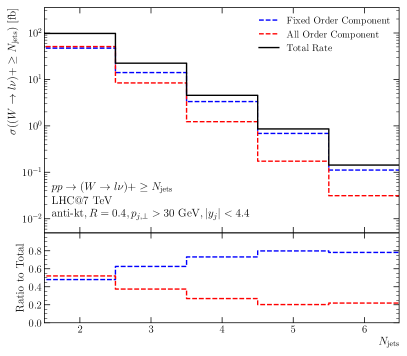
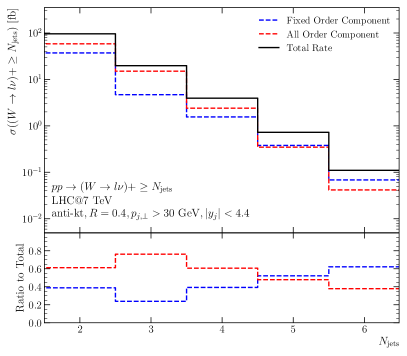
(a)                                                              (b)

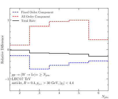
(c)

Figure 21: Inclusive $N_{\mathrm{jets}}$ cross sections for $pp\to(W\to\ell\nu)+\geq N_{\mathrm{jets}}$ where resummation is applied only to LL states (a) and where resummation is applied to all LL and NLL states (b). Also shown in each case is the breakdown into the component where all-order resummation is applied (red, dashed) and the component which remains described at fixed-order only (blue, dashed). Panel (c) shows the relative change in each line. Further details are given in section 3.3.

Fig. 21 shows the inclusive jet rates for $pp\to(W\to\ell\nu)+\geq N_{\mathrm{jets}}$. When resummation is only applied to LL states (fig. 21(a)), one can see that the all-order component successively decreases with each multiplicity which can be understood from a combinatoric argument: for a given set of incoming particles, the number of non-LL states increases with the number of jets, where there remains only one LL state. The new NLL components included in this paper only apply to events with three or more jets, and once included lead to an increase in the all-order component from $W+\geq 2j$ to $W+\geq 3j$ (fig. 21(b)). The rate then decreases for the same reason as above, but remains above half for $W+\geq 4j$. There is only a modest relative effect on the all-order and fixed-order components of the inclusive $W+\geq 2j$ rate (of about 20%) as the change only affects events with three or more jets. Above this, the relative increase in the all-order component is around 80% for $W+\geq 3j$, $W+\geq 4j$ and $W+\geq 5j$ clearly illustrating how much more of the cross section is now controlled by the resummation.

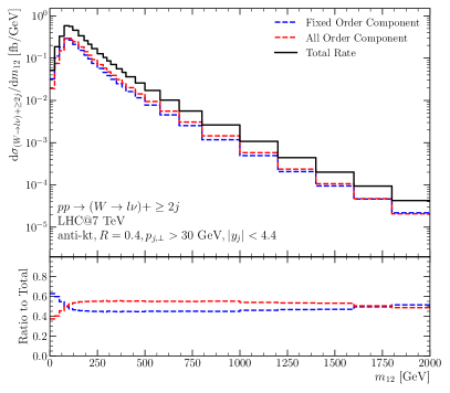
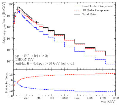
(a)                                                              (b)

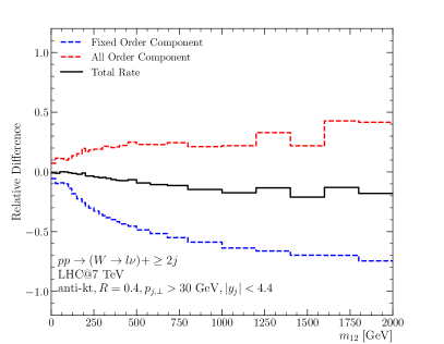
(c)

Figure 22: The differential distribution (black, solid) in the invariant mass of the two leading jets in $pp\to(W\to\ell\nu)\geq 2j$, without and with resummation applied to NLL states. The panels and lines are as in fig. 21.

In fig. 22, we show the comparison now for the invariant mass distribution of the two leading jets in $pp\to(W\to\ell\nu)+\geq 2j$. When all-order corrections are applied to just LL states (fig. 22(a)), we see that the all-order component begins at about 37%, then quickly rises to around 55% by $m_{12}=125$ GeV and remains flat right up to $m_{12}=2$ TeV. When all-order corrections are also added to NLL states (fig. 22(b)), the all-order component begins at a similar value but now quickly rises to much larger values, finally reaching a plateau at about 80% of the total rate for large values of $m_{12}$. Large $m_{12}$ is closely related to the MRK limit, but not identical because the MRK limit requires large invariant mass between all jets and not just between the leading two. Again fig. 22(c) shows the relative difference in each line with the change in the total rate being much smaller than in each component. All three lines show very little relative difference at low $m_{12}$, but then the all-order component shows a relative increase of up to 40% while the fixed-order component increasingly decreases down to about -60%. As the logarithmic corrections grow with invariant mass, we expect this increasing impact with $m_{12}$.

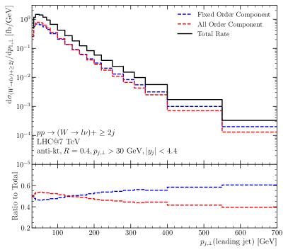
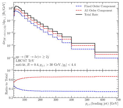
(a)                                                              (b)

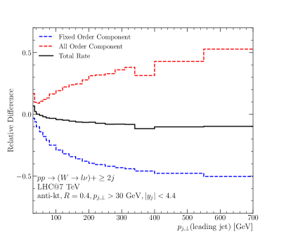
(c)

Figure 23: The differential distribution (black, solid) in the transverse momentum of the leading jet in $pp\to(W\to\ell\nu)\geq 2j$, without and with resummation applied to NLL states. The panels and lines are as in fig. 21.

Finally in fig. 23 we show the transverse momentum distribution of the leading jet in $pp\to(W\to\ell\nu)+\geq 2j$ events. The same distribution for $pp\to(W\to\ell\nu)+\geq 3j$ and $pp\to(W\to\ell\nu)+\geq 4j$ was shown in figs. 13 and 14. Unlike the higher-multiplicity processes, for inclusive 2-jet events one can see that the all-order component is larger than the fixed-order component for low values of $p_{j,\perp}$, which is consistent with the jet rates in fig. 21. It does steadily fall as $p_{j,\perp}$ increases down to 40%. After all-order corrections are applied also to the NLL states though (fig. 23(b)), the behaviour changes and the all-order component rises as a fraction of the total, up to 67% by $p_{j,\perp}=700$ GeV. Again in this variable, the relative difference in the lines is very small at low values of $p_{j,\perp}$ and then the components show much larger differences, up to 50% for the all-order component and down to -50% for the fixed-order component.

References

- (1) ATLAS Collaboration collaboration, G. Aad et al., Measurement of dijet production with a veto on additional central jet activity in collisions at TeV using the ATLAS detector, JHEP 1109 (2011) 053, [1107.1641].
- (2) ATLAS collaboration, G. Aad et al., Measurements of jet vetoes and azimuthal decorrelations in dijet events produced in collisions at using the ATLAS detector, Eur. Phys. J. C74 (2014) 3117, [1407.5756].
- (3) D0 collaboration, V. M. Abazov et al., Studies of boson plus jets production in collisions at TeV, Phys.Rev. D88 (2013) 092001, [1302.6508].
- (4) ATLAS collaboration, M. Aaboud et al., Measurement of the cross-section for electroweak production of dijets in association with a Z boson in pp collisions at = 13 TeV with the ATLAS detector, Phys. Lett. B775 (2017) 206–228, [1709.10264].
- (5) V. S. Fadin, E. Kuraev and L. Lipatov, On the Pomeranchuk Singularity in Asymptotically Free Theories, Phys. Lett. B 60 (1975) 50–52.
- (6) E. A. Kuraev, L. N. Lipatov and V. S. Fadin, Multi - Reggeon processes in the Yang-Mills theory, Sov. Phys. JETP 44 (1976) 443–450.
- (7) E. A. Kuraev, L. N. Lipatov and V. S. Fadin, The Pomeranchuk singularity in nonabelian gauge theories, Sov. Phys. JETP 45 (1977) 199–204.
- (8) I. I. Balitsky and L. N. Lipatov, The Pomeranchuk singularity in quantum chromodynamics, Sov. J. Nucl. Phys. 28 (1978) 822–829.
- (9) J. R. Andersen and J. M. Smillie, Constructing All-Order Corrections to Multi-Jet Rates, JHEP 1001 (2010) 039, [0908.2786].
- (10) J. R. Andersen and J. M. Smillie, The Factorisation of the t-channel Pole in Quark-Gluon Scattering, Phys.Rev. D81 (2010) 114021, [0910.5113].
- (11) J. R. Andersen and J. M. Smillie, Multiple Jets at the LHC with High Energy Jets, JHEP 1106 (2011) 010, [1101.5394].
- (12) J. R. Andersen, T. Hapola and J. M. Smillie, W Plus Multiple Jets at the LHC with High Energy Jets, JHEP 1209 (2012) 047, [1206.6763].
- (13) CMS Collaboration collaboration, S. Chatrchyan et al., Measurement of the inclusive production cross sections for forward jets and for dijet events with one forward and one central jet in collisions at TeV, JHEP 1206 (2012) 036, [1202.0704].
- (14) ATLAS collaboration, G. Aad et al., Measurements of the W production cross sections in association with jets with the ATLAS detector, Eur. Phys. J. C75 (2015) 82, [1409.8639].
- (15) ATLAS collaboration, M. Aaboud et al., Measurements of electroweak production and constraints on anomalous gauge couplings with the ATLAS detector, Eur. Phys. J. C77 (2017) 474, [1703.04362].
- (16) R. Brower, C. E. DeTar and J. Weis, Regge Theory for Multiparticle Amplitudes, Phys.Rept. 14 (1974) 257.
- (17) V. S. Fadin and L. N. Lipatov, Next-to-leading corrections to the BFKL equation from the gluon and quark production, Nucl. Phys. B477 (1996) 767–808, [hep-ph/9602287].
- (18) V. Del Duca, An introduction to the perturbative QCD pomeron and to jet physics at large rapidities, hep-ph/9503226.
- (19) V. Del Duca and E. Glover, The High-energy limit of QCD at two loops, JHEP 10 (2001) 035, [hep-ph/0109028].
- (20) A. Bogdan, V. Del Duca, V. S. Fadin and E. N. Glover, The Quark Regge trajectory at two loops, JHEP 0203 (2002) 032, [hep-ph/0201240].
- (21) J. R. Andersen, T. Hapola, A. Maier and J. M. Smillie, Higgs Boson Plus Dijets: Higher Order Corrections, JHEP 09 (2017) 065, [1706.01002].
- (22) V. Del Duca, A. Frizzo and F. Maltoni, Factorization of tree QCD amplitudes in the high-energy limit and in the collinear limit, Nucl.Phys. B568 (2000) 211–262, [hep-ph/9909464].
- (23) J. R. Andersen, T. Hapola, M. Heil, A. Maier and J. M. Smillie, Higgs-boson plus Dijets: Higher-Order Matching for High-Energy Predictions, JHEP 08 (2018) 090, [1805.04446].
- (24) J. R. Andersen, T. Hapola, M. Heil, A. Maier and J. Smillie, HEJ 2: High Energy Resummation for Hadron Colliders, Comput.Phys.Commun. 245 (2019) , [1902.08430].
- (25) J. R. Andersen, J. J. Medley and J. M. Smillie, plus multiple hard jets in high energy collisions, JHEP 05 (2016) 136, [1603.05460].
- (26) J. R. Andersen, J. D. Cockburn, M. Heil, A. Maier and J. M. Smillie, Finite Quark-Mass Effects in Higgs Boson Production with Dijets at Large Energies, JHEP 04 (2019) 127, [1812.08072].
- (27) J. Alwall, R. Frederix, S. Frixione, V. Hirschi, F. Maltoni, O. Mattelaer et al., The automated computation of tree-level and next-to-leading order differential cross sections, and their matching to parton shower simulations, JHEP 07 (2014) 079, [1405.0301].
- (28) Sherpa collaboration, E. Bothmann et al., Event Generation with Sherpa 2.2, SciPost Phys. 7 (2019) 034, [1905.09127].
- (29) F. Buccioni, S. Pozzorini and M. Zoller, On-the-fly reduction of open loops, Eur. Phys. J. C 78 (2018) 70, [1710.11452].
- (30) ATLAS collaboration, M. Aaboud et al., Measurement of differential cross sections and cross-section ratios for boson production in association with jets at TeV with the ATLAS detector, JHEP 05 (2018) 077, [1711.03296].
- (31) NNPDF collaboration, R. D. Ball et al., Parton distributions from high-precision collider data, Eur. Phys. J. C 77 (2017) 663, [1706.00428].
- (32) A. Buckley, J. Ferrando, S. Lloyd, K. Nordström, B. Page, M. Rüfenacht et al., LHAPDF6: parton density access in the LHC precision era, Eur. Phys. J. C 75 (2015) 132, [1412.7420].