Boosting Monocular Depth Estimation with Lightweight 3D Point Fusion

Abstract

In this paper, we propose enhancing monocular depth estimation by adding 3D points as depth guidance. Unlike existing depth completion methods, our approach performs well on extremely sparse and unevenly distributed point clouds, which makes it agnostic to the source of the 3D points. We achieve this by introducing a novel multi-scale 3D point fusion network that is both lightweight and efficient. We demonstrate its versatility on two different depth estimation problems where the 3D points have been acquired with conventional structure-from-motion and LiDAR. In both cases, our network performs on par with state-of-the-art depth completion methods and achieves significantly higher accuracy when only a small number of points is used while being more compact in terms of the number of parameters. We show that our method outperforms some contemporary deep learning based multi-view stereo and structure-from-motion methods both in accuracy and in compactness.

1 Introduction

Depth estimation from 2D images is a classical computer vision problem that has been mostly tackled with methods from multiple view geometry [15, 45]. Conventional stereo, structure-from-motion and SLAM approaches are already well-established and integrated to many practical applications. However, they rely on feature detection and matching that can be challenging especially when the scene lacks distinct details, and as a result the 3D reconstruction often becomes sparse and incomplete.

More recently, learning-based approaches have been introduced that enable dense depth estimation by exploiting priors learned from training images. In particular, monocular depth estimation that leverages only a single image together with learned priors has become a popular area of research, where deep neural networks are used to implement models that directly predict a depth map for given input image [39, 4, 17, 33, 55, 19]. While the basic idea is simple and attractive, the accuracy of the monocular depth estimation methods is limited by the lack of strong geometric constraints such as parallax. Thus, considerably more accurate depth maps can be achieved with deep learning based multi-view stereo methods [53, 54, 34, 2]. However, the accuracy comes at the cost of increased computational complexity as multiple images need to be aggregated by the network to produce a single depth map.

Another approach for dense depth estimation is to start from depth sensors like LiDARs, and use depth completion to interpolate the missing depth values based on RGB data. Despite of impressive results achieved by recent methods such as [56, 36, 18] they are mainly suitable for cases with relatively high 3D point density, but do not perform well with sparse point clouds.

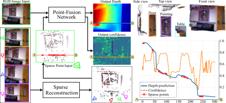
Figure 1: Dense depth prediction on the NYU-Depth-v2 [44] test set. A point cloud is produced by a conventional point-based sparse reconstruction method. The sparse 3D points and a single RGB image are fed to the network to estimate a high-quality depth map. The dense reconstructed point cloud (top right) preserves the geometry well. The chart (bottom right) shows values along the A-B line of the estimated depth map, confidence map, and the sampling points. The estimated depth value tend towards sampling point values. Confidence value around sampling point areas are higher. (All values in the chart are normalized, and sparse point are enhanced for visualization)

In this paper, we start from monocular depth estimation and use a set of 3D points as constraints to obtain high-quality and dense depth maps as illustrated in Figure 1. The main difference of our approach to previous depth completion methods is that the point cloud can be extremely sparse and unevenly sampled, which enables using various methods for acquiring the 3D data, including conventional multi-view stereo, structure-from-motion and SLAM pipelines but also range sensors such as LiDARs. We argue that sparsity is important as it provides flexibility and cost savings to depth sensing. For example, in mobile imaging, existing AR frameworks, i.e. ARCore [23], ARKit [22], and AREngine [24], provide sparse 3D point clouds, while in robotics and autonomous driving applications, low-resolution range sensors become sufficient. To this end, we propose a novel learning-based scheme for fusing RGB and 3D point data. More specifically, our contributions are the following:

• We introduce a novel multi-scale 3D point fusion neural network architecture, which is more lightweight than the existing state-of-the-art depth completion methods while being able to efficiently exploit the geometric constraints provided by a sparse set of 3D points.

• We demonstrate state-of-the-art results on NYU-Depth-v2 and KITTI datasets with a network that uses only a fraction of the number of parameters compared to the other recent architectures.

• We also show that our method combined with 3D point clouds obtained by using COLMAP [43, 42] outperform recent deep learning based multi-view stereo and structure-from-motion methods both in accuracy and in compactness.

2 Related work

Single image depth estimation (SIDE):

SIDE was first introduced by Saxena et al. [41] and it gained momentum from the work by Eigen et al. [10, 9]. Since then, the number of related studies has grown rapidly [28, 14, 37, 40, 30, 26, 17, 4, 12, 39, 33, 32, 29, 19]. At first, the proposed SIDE methods improved the accuracy by employing large architectures [28, 17] and more complex encoding-decoding schemes [4]. Then, they started to diverge into using semantic labels [26], exploiting the relationship between depth and surface normal [37], reformulating as a classification problem [14] or mixing both [40]. Other studies suggested to estimate relative depth [30] or to learn calibration patterns to improve the generalization ability. Recent SIDE approaches exploit monocular priors such as occlusion [39], and planar structures either explicitly [33, 32, 55] or implicitly [19]. Despite these efforts, SIDE still generalizes quite poorly to unseen data. In this work, we leverage SIDE’s ability to produce dense depth estimations and inject it with a small set of depth measurements to boost the accuracy while further shrinking the network size.

Dense depth estimation from sparse depth:

Depth completion is a related problem where the aim is to densify or inpaint an incomplete depth map. Diebel and Thrun [8] is one of the first studies to tackle this problem using Markov random fields. Hawe et al. [16] estimate disparity using wavelet analysis. The problem gained popularity as commodity depth sensors and laser scanners (or LiDARs) become more available. Uhrig et al. [47] proposed sparse convolution to train a sparse invariant network. Jaritz et al. [25] leveraged semantics to train the network at varying sparsity levels. Ma et al. [35] concatenated the sparse depth map to an RGB image, and used this RGBD volume for training. Xu et al. [51] filled in the missing depth values using the depth normal constraint. Imran et al. [21] addressed the depth completion problem using depth coefficients as a representation. Qiu et al. [38] suggested depth and normal fusion using learned attention maps. Methods based on a spatial propagation network (SPN) iterative optimize the dense depth map either in local [6, 7] or non-local [36] affinity. Chen et al. [5] suggested fusing features from an image and 3D points to produce the dense depth. However, these depth completion methods usually aim for outdoor environments and street views where the points come from a LiDAR.

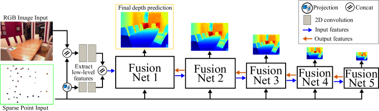
Figure 2: Overview architecture of the 3D point fusion network. Our model consists of five Fusion-Nets that iteratively extract and fuse 2D and 3D features at multiple-scale before predicting the final depth map at the highest spatial resolution.

The difficulty of the depth completion problem much depends on the density of the 3D points used as an input to the algorithm. For example, LiDARs can produce relatively dense and regularly sampled point clouds without large holes, while passive image-based 3D reconstruction techniques, such as stereo or SLAM, result in substantially sparser set of points where the sampling is highly irregular and depends on the surface details. Thus, we argue that depth completion becomes a much harder problem when using a sparse point cloud from image-based reconstruction rather than from a LiDAR, and consequently, it also requires better regularization for the depth. To this end, we introduce a novel 3D fusion point network that efficiently learns to fuse image and geometric features to boost the performance of a monocular depth estimation network. It is a generic approach that can exploit RGB and 3D point data from various sources and environments. It can deal with indoor scenes that are often more diverse and challenging than outdoor environments, but it can be also used for depth estimation from street view scenes. Our work is inspired by [5], but instead of sequentially fusing features at the same resolution, we build a deeper model to extract and fuse features at multiple-scales. This is crucial since [5] has been developed for depth completion of LiDAR data and as shown in our experiments it fails with a sparse set of points whereas thanks to the multi-scale approach our method can achieve reasonable accuracy from a few or even zero depth measurements.

3 Method

An overview of our 3D point fusion network is shown in Figure 2. It is a fully convolutional framework that takes an RGB image and sparse 3D points as inputs to estimate a dense depth map. The 3D points serve as constraints to fix the overall geometry of the depth map produced by the network. To deal with the unstructured 3D point cloud, the points are first projected to the image plane and their $z$ coordinates are used to create a sparse depth map. Next, the RGB image is stacked with the sparse depth to form an RGBD image. We also apply two convolutional layers to the sparse depth and the RGBD image separately. The two outputs are concatenated to build the low-level input features that are fed to the first fusion-net module. The core network consists of five Fusion-Nets that operate at different feature resolutions. Each Fusion-Net contains a feature fusion encoder (E), a confidence predictor (C), a decoder (D), and a refinement (R) module as illustrates in Figure 3. We describe these modules in the following subsections and finish this section by giving details about our loss function.

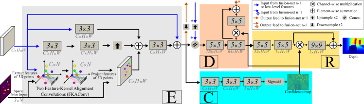
Figure 3: Details of Fusion-Net $n\in[1,5]$, where $n$ is the scale resolution. Main components include the feature fusion encoder (E), confidence predictor (C), decoder (D) and refinement (R) are color coded as gray, cyan, orange and yellow, respectively.

3.1 Feature Fusion Encoder

Convolutional neural networks are good in processing regularly sampled data in a tensor form. Because our input point clouds are sparse and they represent geometric constraints unlike the image data, we cannot just rely on simple concatenation to fuse the information, but we need better representations. Inspired by a recent depth completion method [5], we design a feature fusion encoder to extract low-level features from RGB images and 3D points.

Our feature fusion encoder takes a 3D tensor ($C\times H\times W$) and a set of sparse points ($3\times N$) as inputs, where $C$ is the number of feature channels, $H$ and $W$ are the height and width of the input tensor, and $N$ is the number of 3D points. The output is a 3D tensor with a similar shape to the input tensor. Details of the feature fusion encoder are shown in the gray box of Figure 3. It consists of two 2D branches, one 3D branch, and one convolutional layer for feature fusion.

The 2D convolutional branches: The 2D branches are convolved at two different resolutions to learn multi-scale representations from the input 3D tensor. The first 2D branch has one convolutional layer with stride one to extract features at the same size as the input volume. The second 2D branch is a cascade of a stride two convolutional, a stride one convolutional, and an upsampling layer to obtain coarser features of the input tensor. The two outputs are summed to aggregate appearance features at different resolutions.

The 3D point convolution branch: The 3D branch aims to extract structural features from the sparse points. This is difficult for 2D convolutions that operate on local neighbors as 3D points are located on an irregular grid. Therefore, we utilize the feature-kernel alignment convolution (FKAConv) [3] that operates directly on 3D points to avoid this problem. The key idea of the FKAConv is to learn a linear transformation to align the neighboring points with the grid-like kernel. After that, it performs a weighted sum between this kernel and the features of the 3D points. One can see that 2D convolution is a special case where the learned linear transformation is always an identity matrix.

As shown in Figure 3, our 3D branch consists of two FKAConv layers. We first extract the features of the 3D points from the input tensor using their projected 2D indices on the image plane. This volume has the size of $C\times N$. Next, we feed the point features and their 3D coordinates to the FKAConv layers. FKAConv selects a set of k-neighboring points for every input point and learns a transformation matrix to align the 3D points with its kernel. The point features are then convolved with the aligned 3D points to produce a 2D tensor of shape $C\times N$. The output features are projected back to an empty 3D tensor of size $C\times H\times W$ using the projected 2D indices. Features of other positions are set to zero.

2D-3D Feature Fusion: Output volumes from the 2D and 3D branches have the same shape as the input tensor ($C\times H\times W$). Therefore, to fuse these features, we sum them together before applying a 2D convolutional layer to output a 3D tensor of the size $C\times H\times W$. Finally, we add a residual connection to avoid vanishing gradient during training.

3.2 Encoder, Decoder, and Confidence Predictor modules

Encoder and Decoder Module: Designing efficient decoder and refinement modules is essential for the depth estimation problem [13, 50]. A common practice is to create large and complex decoders to produce accurate depth maps with sharp edges and fine details. However, we argue that by iteratively fusing relevant depth measurements from the 3D points with appearance features from image pixels, we can significantly reduce the size of our decoder and refinement designs. That is, our decoder and refinement modules have only two convolutional layers for each component. To simplify further, we use the same decoder and refinement designs for all Fusion-Nets.

As shown in the orange box of Figure 3, the decoder transforms the fused features from the encoder before feeding them to the refinement module (the yellow box in Figure 3). We then initially obtain an output tensor of the decoder and a depth map. The estimated confidence map later modifies these two outputs.

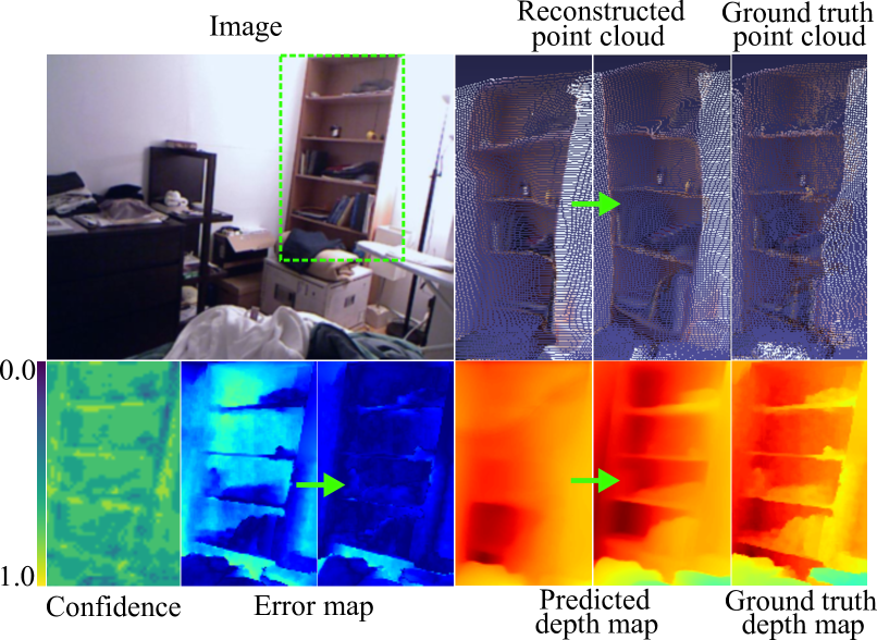
Figure 4: Depth map rectification by predicted confidence (green arrow). Confidence map values range from 0.0 (low) to 1.0 (high).

Table 1: Evaluation on the NYU dataset. Metrics mark $\downarrow$ mean lower is better while $\uparrow$ is otherwise. Methods with ^‡ are trained using extra data. Figures with ^⋆ indicates 3D COLMAP points while figures without ^⋆ are obtained using randomly sampled points from GT depths.

Architecture		#3D pts	#params	REL$\downarrow$	RMSE$\downarrow$	$\boldsymbol{\delta_{1}}$$\uparrow$	$\boldsymbol{\delta_{2}}$$\uparrow$	$\boldsymbol{\delta_{3}}$$\uparrow$
SharpNet	Ramam.’19‡ [39]	0	80.4M	0.139	0.502	0.836	0.966	0.993
Revisited mono-depth	Hu’19 [17]	0	157.0M	0.115	0.530	0.866	0.975	0.993
SARPN	Chen’19 [4]	0	210.3M	0.111	0.514	0.878	0.977	0.994
VNL	Yin’19 [55]	0	114.2M	0.108	0.416	0.875	0.976	0.994
DAV	Huynh’20 [19]	0	25.1M	0.108	0.412	0.882	0.980	0.996
Point-Fusion	Ours	0	8.7M	0.128	0.505	0.847	0.971	0.994
NLSPN	Park’20 [36]	2	25.8M	0.300	1.152	0.393	0.697	0.879
Point-Fusion	Ours	2	8.7M	0.109	0.470	0.875	0.975	0.995
NLSPN	Park’20 [36]	32	25.8M	0.114	0.554	0.825	0.947	0.985
Point-Fusion	Ours	32	8.7M	0.057	0.319	0.963	0.992	0.998
Sparse & Dense	Jaritz’18 [25]	200	58.3M	0.050	0.194	0.930	0.960	0.991
S2D	Ma’18 [35]	200	42.8M	0.044	0.230	0.971	0.994	0.998
GuideNet	Tang’20 [46]	200	63.3M	0.024	0.142	0.988	0.998	1.000
NLSPN	Park’20 [36]	200	25.8M	0.019	0.136	0.989	0.998	0.999
Point-Fusion	Ours	200	8.7M	0.015	0.112	0.995	0.999	1.000
FuseNet	Chen’19 [5]	500	1.9M	0.318	0.859	0.688	0.789	0.887
CSPN	Cheng’18 [6]	500	18.5M	0.016	0.117	0.992	0.999	1.000
DeepLiDAR	Qiu’19 [38]	500	53.4M	0.022	0.115	0.993	0.999	1.000
Depth Coefficients	Imran’19 [21]	500	45.7M	0.013	0.118	0.994	0.999	-
DepthNormal	Xu’19 [51]	500	29.1M	0.018	0.112	0.995	0.999	1.000
CSPN++	Cheng’20 [7]	500	28.8M	-	0.116	-	-	-
GuideNet	Tang’20 [46]	500	63.3M	0.015	0.101	0.995	0.999	1.000
NLSPN	Park’20 [36]	500	25.8M	0.012	0.092	0.996	0.999	1.000
Point-Fusion	Ours	500	8.7M	0.014	0.090	0.996	0.999	1.000
MVSNet	Yao’18 [53]	-	124.5M	0.043	0.162	0.940	0.972	0.996
CodeSLAM	Bloesch’18 [2]	-	66.3M	0.096	0.251	0.910	0.962	0.989
Consistent depth	Luo’20 [34]	-	178.2M	0.086	0.345	0.916	0.959	0.984
NLSPN	Park’20 [36]	500⋆	25.8M	0.042	0.144	0.949	0.981	0.999
Point-Fusion	Ours	500⋆	8.7M	0.022	0.126	0.994	0.999	1.000

Confidence Predictor: Although the input 3D sparse points provide useful depth measurements, they can also contain noise. Hence, we proposed a simple yet efficient confidence predictor to attenuate the effect of noise. As illustrated in the cyan box of Figure 3, the output volumes from the feature fusion encoder are fed to three convolutional layers followed by a sigmoid to output the probability for every pixel. This information is then used to alter the initial depth map and the output features of the decoder. Moreover, we add residual connections at the end of the decoder and refinement blocks to prevent the vanishing gradient problem and regularize the confidence map’s errors. The initial depth map is corrected based on the confidence map, as illustrated in Figure 4.

3.3 Multi-scale Loss function

We calculate the loss at multiple feature resolutions to train our network. The full loss is defined as:

$$\mathcal{L}=\sum_{i=1}^{n=5}\gamma^{i}(\mathcal{L}^{i}_{log}+\mu\mathcal{L}^{i}_{grad}+\theta\mathcal{L}^{i}_{norm})$$ (1)

where $n$ is the number of resolution scales and $\gamma^{i}\in\mathbb{R}^{+}$ is the loss weight at scale $i$, $\mathcal{L}_{log}$ is a variation of the $L_{1}$ norm that minimizes error on the sparse depth pixels, $\mathcal{L}_{grad}$ optimizes the error on edge structures, and $\mathcal{L}_{norm}$ penalizes angular error between the ground truth and predicted normal surfaces. These loss terms were introduced by Hu et al.  [17] and widely adopted by state-of-art monocular depth estimation methods [4, 19]. Subsection 4.2 describes in detail how the network is trained using these loss functions.

4 Experiments

In this section, we evaluate the performance of the proposed method and compare it with several baselines on the NYU-Depth-v2 and KITTI datasets.

4.1 Dataset and Evaluation metrics

Datasets.

The NYU-Depth-v2 dataset contains approximately $120K$ RGB-D images recorded from 464 indoor scenes. We extract the raw RGB frames from the original videos and reconstruct sparse 3D point clouds using the COLMAP [42, 43] structure-from-motion software. COLMAP is also used to extract the camera poses for multi-view stereo methods. The 3D points are back-projected to each input view to obtain a sparse set of depth values. We use 60K images for training and 654 images from the official test set for evaluating the methods. For KITTI, we utilize 85K images for training, 1000 images for validation and 1000 images for testing on the KITTI depth completion benchmark [47].

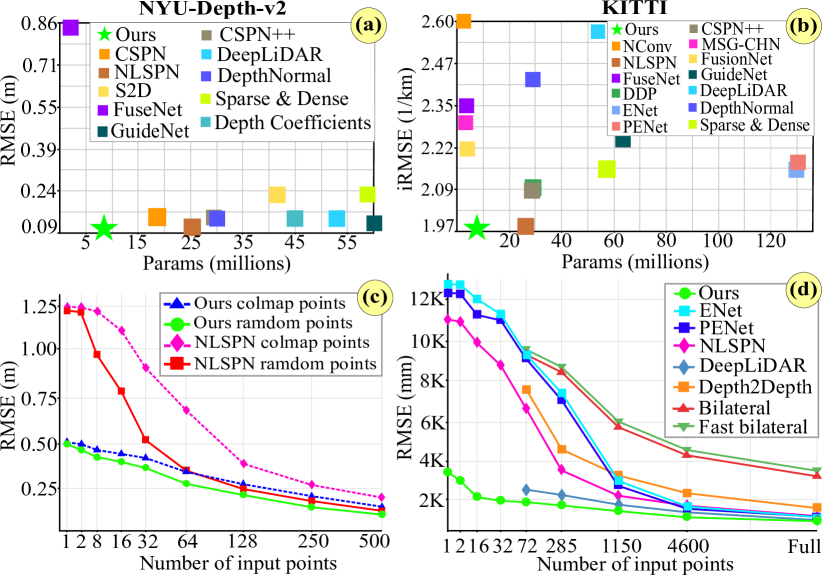
Figure 5: Top: RMSE and iRMSE metrics v. the number of parameters plots for recent depth completion methods on NYU-Depth-v2 (a) and KITTI (b). Bottom: RMSE metrics for different sparsity and patterns for NYU-Depth-v2 (c) and KITTI (d).

Evaluation metrics.

We report the results in terms of standard metrics for each dataset. For NYU-Depth-v2 we compute the mean absolute relative error (REL), root mean square error (RMSE), and thresholded accuracy ($\delta_{i}$). For KITTI, we also calculate RMSE plus mean absolute error (MAE), root mean square error (iRMSE) and mean absolute error (iMAE) of the inverse depth values. The detailed definitions of the measures are provided in the supplementary material.

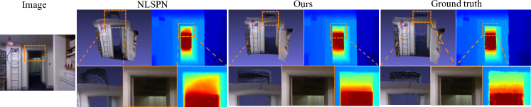
Figure 6: Qualitative results on NYU-v2 test set. Note that all methods use 200 randomly sampled 3D points as input.

4.2 Implementation details

The proposed model is trained for 150 epochs on a single TITAN RTX using batch size of 32, the Adam optimizer [27] with $(\beta_{1},\beta_{2},\epsilon)=(0.9,0.999,10^{-8})$, and the loss function presented in (1). The initial learning rate is $1.2*10^{-4}$, but from epoch 10 the learning is reduced by $6\%$ per $5$ epochs. We set the number of scales $n$ in (1) to 5, weight loss coefficients $\mu,\theta$ to $1.0$, and the scale weight losses $\gamma^{1},\gamma^{2},\gamma^{3},\gamma^{4},\gamma^{5}$ to $1.0,0.75,0.5,0.25$ and $0.125$ respectively. To remove the effect of the arbitrary scale of the COLMAP points, we center and normalize the 3D inputs to a unit sphere before the training. During training, we augment the input RGB and ground truth depth images using random rotation ([-5.0, +5.0] degrees), horizontal flip, rectangular window droppings, and colorization (RGB only).

4.3 Comparison with State-of-the-art

The proposed method is related to multiple partially overlapping problems and, therefore, we compare it with several baseline methods in monocular depth estimation [39, 17, 4, 55, 19], depth completion [5, 6, 7, 11, 18, 20, 21, 25, 31, 35, 36, 38, 46, 48, 51, 52], deep multi-view stereo [53], deep structure-from-motion/SLAM [34, 2]. The baseline results are obtained using the pre-trained models [4, 17, 39, 55, 34, 18, 11], re-training using the official NYU-v2 [2, 35, 36, 53] code, using our own re-implementations [19, 25], and from the original papers [7, 38, 51, 21, 46, 52].

NYU-Depth-v2.

The performance metrics, computed between the estimated depth maps and the ground truth, are provided in Table 1. In addition, we report the number of method parameters, and the number of 3D points used in the estimation. Compared to monocular depth estimation studies, the proposed method provides a substantial improvement according to all metrics. For instance, REL, RMSE and thresholded accuracy ($\delta_{i}$) are improved by $47\%,22.5\%$ and $10\%$, respectively, by using only $35\%$ of the model parameters and 32 additional 3D points. Table 1 also shows that our method produces results close to state-of-the-art even without using any 3D inputs, while 2 points are already enough to be on par with the baseline approaches.

Table 2: Evaluation results on the test set of the KITTI depth completion benchmark. Performance figures are color-coded as red, green, and blue, corresponding to first, second and third best results, respectively.

Architecture #param RMSE MAE iRMSE iMAE Sparse&Dense [25] 58.3M 917.6 234.8 2.17 0.95 NConv [11] 0.36M 829.9 233.2 2.60 1.03 DepthNormal [51] 29.1M 777.1 235.2 2.42 1.13 FusionNet [48] 2.5M 772.9 215.1 2.19 0.95 FuseNet [5] 1.9M 752.9 221.2 2.34 1.14 DeepLiDAR [38] 53.4M 748.4 226.5 2.56 1.15 DDP [52] 29.1M 832.9 203.9 2.10 0.85 MSG-CHN [31] 1.25M 762.2 220.4 2.30 0.98 CSPN++ [7] 28.8M 743.7 209.3 2.07 0.90 NLSPN [36] 25.8M 741.7 199.6 1.99 0.84 GuideNet [46] 63.3M 736.2 218.8 2.25 0.99 ENet [18] 131.6M 741.3 216.3 2.14 0.95 PENet [18] 133.7M 730.1 210.6 2.17 0.94 TWISE_2 [20] - 840.2 195.6 2.08 0.82 Point-Fusion(Ours) 8.7M 741.9 201.1 1.97 0.85

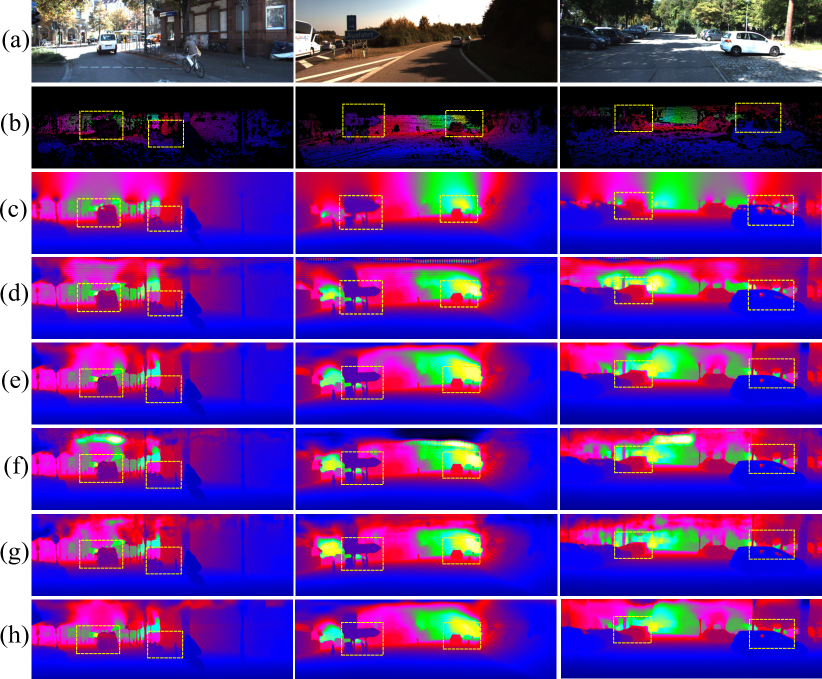
Figure 7: Examples from the KITTI validation set. Input images (a), ground truth LiDAR (b). Results from (c) Depth2Depth [56], (d) DeepLiDAR [38], (e) NLSPN [36], (f) ENet [18], (g) PENet [18], and (h) the proposed method.

Compared to the depth completion methods, we obtain state-of-the-art performance while using clearly less model parameters as shown in Figure 5 a). The best performing baselines, NLSPN [36], DepthNormal [51], GuideNet [46] use $2.9$, $3.4$, and $7.3$ times more parameters compared to our method, respectively. Instead of using the explicit 3D points, the multi-view stereo [53], structure-from-motion [34], and SLAM [2] methods utilise multiple RGB images with camera poses. The results in Table 1 indicate that the proposed model outperforms also these methods using only a fraction of the model parameters.

Figure 6 shows qualitative results of the predicted depth maps and reconstructed points cloud for our method and for [36]. The baseline [36] results are obtained using the pre-trained model provided by the authors. Although both methods produce high quality depth maps, the proposed model is better in recovering fine details in challenging regions and introduces less distortions on flat surfaces.

We also provide examples where we reconstructed a very sparse set of 3D points (32 points) from two images and utilized those as the 3D inputs. The dense depth maps obtained with this setting using our method, NLSPN [36] and MVSNet [53] are illustrated in Figure 8. We argue that state-of-the-art depth completion methods are usually vulnerable in high sparsity cases, while deep multi-view stereo performance degrades with less input views. One the other hand, our method produces high quality depth maps with significantly less distortions. Additional results are provided in the supplementary material.

KITTI.

To demonstrate the versatility of the proposed method, we also experiment with outdoor data. For this purpose, we train and test our model with the KITTI depth completion dataset [47], in which we perform on par with state-of-the-art methods using a significantly smaller number of parameters as shown in Table 2. We notice that there is a clear trade-off between model parameters and performance as shown in Figure 5 b). Figure 7 presents qualitative comparison with baseline methods. The proposed method produces finer depth details as emphasized in the highlight areas. However, the difference is largest with a small number of input 3D points as depicted in Figure 5 d). The results suggest that high-quality depth maps can be obtained by using only a few LiDAR points enabling more cost efficient solutions. Additional results are also added to the supplementary material.

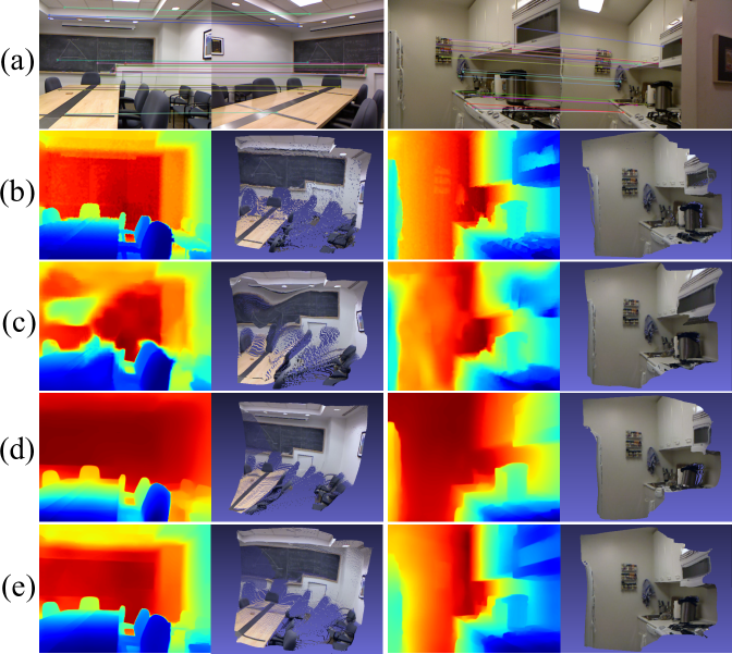
Figure 8: NYU test set examples (a). Dense depth maps and reconstructed point cloud from two images: (b) ground truth, (c) NLSPN [36], (d) MVSNet [53], and (e) the proposed method.

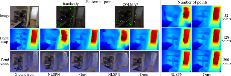
Figure 9: Qualitative comparison of the pattern (left) and quantity (right) of input points. Random points are sampled from the dense ground truth depth map. For COLMAP points, we extract the image frames from raw NYU data and run COLMAP to obtain the points. The pattern and number of points are kept similar in all cases. Left: the number of points in use is 64. Results in the first row show the random input point have better spatial distribution than COLMAP points since they cover flat surfaces like walls, floors or doors. Right: example results show the predicted depth maps using random sampled set of 32, 128 and 200 points respectively. Our method perform consistently better than NLSPN [36] in all cases. (Points are enhanced for visualization)

4.4 Ablation studies

Number and sampling of input 3D points.

To analyze how the quantity and spatial distribution of the input 3D point affect the results, we performed experiments with varying 3D point patterns. For this purpose we generate sparse point sets by randomly sampling from the dense ground truth or from COLMAP output. We expect that by sampling from dense depth map provides better results compared to the COLMAP points. This is because, dense depth map covers also flat textureless surfaces such as walls, floor, and doors. However, such points might not be easy to obtain in practice, whereas COLMAP points represent location which are often reconstructed by SfM or SLAM methods.

Figure 5 c) presents the RMSE errors for different number of input points for both types. The results confirm the initial assumption that sampling from a dense depth map results in better performance. Moreover, we notice that the proposed method obtains higher accuracy compared to NLSPN [36] with all point sets. In fact, we obtain similar performance using COLMAP points as NLSPN [36] using points from the dense depth map. Figure 9 shows qualitative comparison with NLSPN [36].

Confidence predictor.

We study the impact of the confidence predictor module by training our method with and without this component. We report the results in Table 3. When compared to a model without the confidence map, REL improves $\sim 3.5\%$, and RMSE $\sim 7.2\%$.

Table 3: Ablation studies of models without and with the confidence predictor (CP) on NYU-Depth-v2.

Training	REL$\downarrow$	RMSE$\downarrow$	$\boldsymbol{\delta_{1}}$$\uparrow$	$\boldsymbol{\delta_{2}}$$\uparrow$	$\boldsymbol{\delta_{3}}$$\uparrow$
w/o CP	0.015	0.097	0.994	0.997	0.999
w/ CP	0.014	0.090	0.996	0.999	1.000

Multi-scale Fusion-Net.

We assess how the number of Fusion-Nets affects the performance. For this purpose, we train our model using $2-6$ Fusion-Nets. The corresponding RMSE for the NYU-Depth-v2 test set are provided in Table 4. The results improve by increasing the number of Fusion-Net to five and degrade after that. As each Fusion-Net perform at a different feature resolution, we argue that five is the optimal cascade size for the network to learn the geometric features from the 3D inputs.

Table 4: Performance of our model using different numbers of Fusion-Net on NYU-Depth-v2.

# of FusionNet	2	3	4	5	6
RMSE	0.105	0.097	0.094	0.090	0.093

3D point convolutions.

We study the effect of different types of 3D point convolutions by training our model using the deep parametric continuous convolution (PCC) [49] and the FKAConv [3]. The results are provided in Table 5. The comparison with the PCC shows that the FKAConv module reduces the network size by $\sim 5\%$ while slightly improves the performance by $\sim 3\%$. We also trained our model without the 3D branch and the performance dropped considerably as shown in Table 5.

Table 5: Performance of our model applying different types of 3D point convolutions on NYU-Depth-v2.

Training	#params	REL$\downarrow$	RMSE$\downarrow$	$\boldsymbol{\delta_{1}}$$\uparrow$	$\boldsymbol{\delta_{2}}$$\uparrow$
w/o 3D branch	7.6M	0.044	0.196	0.980	0.993
w/ PCC	9.1M	0.015	0.096	0.994	0.996
w/ FKAConv	8.7M	0.014	0.090	0.996	0.999

5 Conclusion

We propose a novel and pragmatic approach that fuses RGB monocular depth estimation with information from a sparse set of 3D points for dense depth estimation. Experiments on common indoor and outdoor datasets show that we achieve state-of-the-art results while being compact in terms of the number of parameters. Moreover, our method can also produce, unlike the competitors, high-quality depth maps using an extremely sparse set of 3D points, which enables a cost-efficient solution for obtaining accurate depth maps for various applications where dense depth is needed.

References

- [1] Jonathan T Barron and Ben Poole. The fast bilateral solver. In European Conference on Computer Vision, pages 617–632. Springer, 2016.
- [2] Michael Bloesch, Jan Czarnowski, Ronald Clark, Stefan Leutenegger, and Andrew J Davison. Codeslam—learning a compact, optimisable representation for dense visual slam. In Proceedings of the IEEE conference on computer vision and pattern recognition, pages 2560–2568, 2018.
- [3] Alexandre Boulch, Gilles Puy, and Renaud Marlet. FKAConv: Feature-Kernel Alignment for Point Cloud Convolution. In 15th Asian Conference on Computer Vision (ACCV 2020), 2020.
- [4] Xiaotian Chen, Xuejin Chen, and Zheng-Jun Zha. Structure-aware residual pyramid network for monocular depth estimation. In Proceedings of the 28th International Joint Conference on Artificial Intelligence, pages 694–700. AAAI Press, 2019.
- [5] Yun Chen, Bin Yang, Ming Liang, and Raquel Urtasun. Learning joint 2d-3d representations for depth completion. In Proceedings of the IEEE International Conference on Computer Vision, pages 10023–10032, 2019.
- [6] Xinjing Cheng, Peng Wang, and Ruigang Yang. Depth estimation via affinity learned with convolutional spatial propagation network. In Proceedings of the European Conference on Computer Vision (ECCV), pages 103–119, 2018.
- [7] Xinjing Cheng, Peng Wang, and Ruigang Yang. Learning depth with convolutional spatial propagation network. IEEE transactions on pattern analysis and machine intelligence, 2019.
- [8] James Diebel and Sebastian Thrun. An application of markov random fields to range sensing. In Advances in neural information processing systems, pages 291–298, 2006.
- [9] David Eigen and Rob Fergus. Predicting depth, surface normals and semantic labels with a common multi-scale convolutional architecture. In Proceedings of the IEEE International Conference on Computer Vision, pages 2650–2658, 2015.
- [10] David Eigen, Christian Puhrsch, and Rob Fergus. Depth map prediction from a single image using a multi-scale deep network. In Advances in neural information processing systems, pages 2366–2374, 2014.
- [11] Abdelrahman Eldesokey, Michael Felsberg, and Fahad Shahbaz Khan. Confidence propagation through cnns for guided sparse depth regression. IEEE transactions on pattern analysis and machine intelligence, 2019.
- [12] Jose M Facil, Benjamin Ummenhofer, Huizhong Zhou, Luis Montesano, Thomas Brox, and Javier Civera. Cam-convs: camera-aware multi-scale convolutions for single-view depth. In Proceedings of the IEEE Conference on Computer Vision and Pattern Recognition, pages 11826–11835, 2019.
- [13] Zhicheng Fang, Xiaoran Chen, Yuhua Chen, and Luc Van Gool. Towards good practice for cnn-based monocular depth estimation. In The IEEE Winter Conference on Applications of Computer Vision, pages 1091–1100, 2020.
- [14] Huan Fu, Mingming Gong, Chaohui Wang, Kayhan Batmanghelich, and Dacheng Tao. Deep ordinal regression network for monocular depth estimation. In Proceedings of the IEEE Conference on Computer Vision and Pattern Recognition, pages 2002–2011, 2018.
- [15] Richard Hartley and Andrew Zisserman. Multiple view geometry in computer vision. Cambridge university press, 2003.
- [16] Simon Hawe, Martin Kleinsteuber, and Klaus Diepold. Dense disparity maps from sparse disparity measurements. In 2011 International Conference on Computer Vision, pages 2126–2133. IEEE, 2011.
- [17] Junjie Hu, Mete Ozay, Yan Zhang, and Takayuki Okatani. Revisiting single image depth estimation: Toward higher resolution maps with accurate object boundaries. In IEEE Winter Conf. on Applications of Computer Vision (WACV), 2019.
- [18] Mu Hu, Shuling Wang, Bin Li, Shiyu Ning, Li Fan, and Xiaojin Gong. Towards precise and efficient image guided depth completion. ICRA, 2021.
- [19] Lam Huynh, Phong Nguyen-Ha, Jiri Matas, Esa Rahtu, and Janne Heikkilä. Guiding monocular depth estimation using depth-attention volume. In European Conference on Computer Vision, pages 581–597. Springer, 2020.
- [20] Saif Imran, Xiaoming Liu, and Daniel Morris. Depth completion with twin-surface extrapolation at occlusion boundaries. In In Proceeding of IEEE Computer Vision and Pattern Recognition, Nashville, TN, June 2021.
- [21] Saif Imran, Yunfei Long, Xiaoming Liu, and Daniel Morris. Depth coefficients for depth completion. In 2019 IEEE/CVF Conference on Computer Vision and Pattern Recognition (CVPR), pages 12438–12447. IEEE, 2019.
- [22] Apple Inc. ARKit 2, Accessed 28 Feb 2019.
- [23] Google Inc. ARCore Resources, Released 01 Mar 2018.
- [24] Huawei Inc. AREngine, Released 30 June 2019.
- [25] Maximilian Jaritz, Raoul De Charette, Emilie Wirbel, Xavier Perrotton, and Fawzi Nashashibi. Sparse and dense data with cnns: Depth completion and semantic segmentation. In 2018 International Conference on 3D Vision (3DV), pages 52–60. IEEE, 2018.
- [26] Jianbo Jiao, Ying Cao, Yibing Song, and Rynson Lau. Look deeper into depth: Monocular depth estimation with semantic booster and attention-driven loss. In Proceedings of the European Conference on Computer Vision (ECCV), pages 53–69, 2018.
- [27] Diederik P Kingma and Jimmy Ba. Adam: A method for stochastic optimization. arXiv preprint arXiv:1412.6980, 2014.
- [28] Iro Laina, Christian Rupprecht, Vasileios Belagiannis, Federico Tombari, and Nassir Navab. Deeper depth prediction with fully convolutional residual networks. In 2016 Fourth International Conference on 3D Vision (3DV), pages 239–248. IEEE, 2016.
- [29] Jin Han Lee, Myung-Kyu Han, Dong Wook Ko, and Il Hong Suh. From big to small: Multi-scale local planar guidance for monocular depth estimation. arXiv preprint arXiv:1907.10326, 2019.
- [30] Jae-Han Lee and Chang-Su Kim. Monocular depth estimation using relative depth maps. In Proceedings of the IEEE Conference on Computer Vision and Pattern Recognition, pages 9729–9738, 2019.
- [31] Ang Li, Zejian Yuan, Yonggen Ling, Wanchao Chi, Chong Zhang, et al. A multi-scale guided cascade hourglass network for depth completion. In Proceedings of the IEEE/CVF Winter Conference on Applications of Computer Vision, pages 32–40, 2020.
- [32] Chen Liu, Kihwan Kim, Jinwei Gu, Yasutaka Furukawa, and Jan Kautz. Planercnn: 3d plane detection and reconstruction from a single image. In Proceedings of the IEEE Conference on Computer Vision and Pattern Recognition, pages 4450–4459, 2019.
- [33] Chen Liu, Jimei Yang, Duygu Ceylan, Ersin Yumer, and Yasutaka Furukawa. Planenet: Piece-wise planar reconstruction from a single rgb image. In Proceedings of the IEEE Conference on Computer Vision and Pattern Recognition, pages 2579–2588, 2018.
- [34] Xuan Luo, Jia-Bin Huang, Richard Szeliski, Kevin Matzen, and Johannes Kopf. Consistent video depth estimation. ACM Transactions on Graphics (Proceedings of ACM SIGGRAPH), 39(4), 2020.
- [35] Fangchang Mal and Sertac Karaman. Sparse-to-dense: Depth prediction from sparse depth samples and a single image. In 2018 IEEE International Conference on Robotics and Automation (ICRA), pages 1–8. IEEE, 2018.
- [36] Jinsun Park, Kyungdon Joo, Zhe Hu, Chi-Kuei Liu, and In So Kweon. Non-local spatial propagation network for depth completion. In Proc. of European Conference on Computer Vision (ECCV), 2020.
- [37] Xiaojuan Qi, Renjie Liao, Zhengzhe Liu, Raquel Urtasun, and Jiaya Jia. Geonet: Geometric neural network for joint depth and surface normal estimation. In Proceedings of the IEEE Conference on Computer Vision and Pattern Recognition, pages 283–291, 2018.
- [38] Jiaxiong Qiu, Zhaopeng Cui, Yinda Zhang, Xingdi Zhang, Shuaicheng Liu, Bing Zeng, and Marc Pollefeys. Deeplidar: Deep surface normal guided depth prediction for outdoor scene from sparse lidar data and single color image. In The IEEE Conference on Computer Vision and Pattern Recognition (CVPR), June 2019.
- [39] Michael Ramamonjisoa and Vincent Lepetit. Sharpnet: Fast and accurate recovery of occluding contours in monocular depth estimation. The IEEE International Conference on Computer Vision (ICCV) Workshops, 2019.
- [40] Haoyu Ren, Mostafa El-khamy, and Jungwon Lee. Deep robust single image depth estimation neural network using scene understanding. In Proceedings of the IEEE Conference on Computer Vision and Pattern Recognition Workshops, pages 37–45, 2019.
- [41] Ashutosh Saxena, Sung H Chung, and Andrew Y Ng. Learning depth from single monocular images. In Advances in neural information processing systems, pages 1161–1168, 2006.
- [42] Johannes Lutz Schönberger and Jan-Michael Frahm. Structure-from-motion revisited. In Conference on Computer Vision and Pattern Recognition (CVPR), 2016.
- [43] Johannes Lutz Schönberger, Enliang Zheng, Marc Pollefeys, and Jan-Michael Frahm. Pixelwise view selection for unstructured multi-view stereo. In European Conference on Computer Vision (ECCV), 2016.
- [44] Nathan Silberman, Derek Hoiem, Pushmeet Kohli, and Rob Fergus. Indoor segmentation and support inference from rgbd images. In European Conference on Computer Vision, pages 746–760. Springer, 2012.
- [45] Richard Szeliski. Structure from motion. In Computer Vision, pages 303–334. Springer, 2011.
- [46] Jie Tang, Fei-Peng Tian, Wei Feng, Jian Li, and Ping Tan. Learning guided convolutional network for depth completion. IEEE Transactions on Image Processing, 30:1116–1129, 2020.
- [47] Jonas Uhrig, Nick Schneider, Lukas Schneider, Uwe Franke, Thomas Brox, and Andreas Geiger. Sparsity invariant cnns. In 2017 international conference on 3D Vision (3DV), pages 11–20. IEEE, 2017.
- [48] Wouter Van Gansbeke, Davy Neven, Bert De Brabandere, and Luc Van Gool. Sparse and noisy lidar completion with rgb guidance and uncertainty. In 2019 16th International Conference on Machine Vision Applications (MVA), pages 1–6. IEEE, 2019.
- [49] Shenlong Wang, Simon Suo, Wei-Chiu Ma, Andrei Pokrovsky, and Raquel Urtasun. Deep parametric continuous convolutional neural networks. In Proceedings of the IEEE Conference on Computer Vision and Pattern Recognition, pages 2589–2597, 2018.
- [50] Zbigniew Wojna, Vittorio Ferrari, Sergio Guadarrama, Nathan Silberman, Liang-Chieh Chen, Alireza Fathi, and Jasper Uijlings. The devil is in the decoder: Classification, regression and gans. International Journal of Computer Vision, 127(11-12):1694–1706, 2019.
- [51] Yan Xu, Xinge Zhu, Jianping Shi, Guofeng Zhang, Hujun Bao, and Hongsheng Li. Depth completion from sparse lidar data with depth-normal constraints. In Proceedings of the IEEE International Conference on Computer Vision, pages 2811–2820, 2019.
- [52] Yanchao Yang, Alex Wong, and Stefano Soatto. Dense depth posterior (ddp) from single image and sparse range. In Proceedings of the IEEE Conference on Computer Vision and Pattern Recognition, pages 3353–3362, 2019.
- [53] Yao Yao, Zixin Luo, Shiwei Li, Tian Fang, and Long Quan. Mvsnet: Depth inference for unstructured multi-view stereo. European Conference on Computer Vision (ECCV), 2018.
- [54] Yao Yao, Zixin Luo, Shiwei Li, Tianwei Shen, Tian Fang, and Long Quan. Recurrent mvsnet for high-resolution multi-view stereo depth inference. Computer Vision and Pattern Recognition (CVPR), 2019.
- [55] Wei Yin, Yifan Liu, Chunhua Shen, and Youliang Yan. Enforcing geometric constraints of virtual normal for depth prediction. In The IEEE International Conference on Computer Vision (ICCV), 2019.
- [56] Yinda Zhang and Thomas Funkhouser. Deep depth completion of a single rgb-d image. In Proceedings of the IEEE Conference on Computer Vision and Pattern Recognition, pages 175–185, 2018.