\zxrsetup

tozreflabel=false, toltxlabel=true,

Reduced-Rank Tensor-on-Tensor Regression and Tensor-variate Analysis of Variance

Carlos Llosa-Vite and Ranjan Maitra C. Llosa-Vite and R. Maitra are with the Department of Statistics at Iowa State University, Ames, Iowa 50011, USA. e-mail: {cllosa,maitra}@iastate.edu.
Abstract

Fitting regression models with many multivariate responses and covariates can be challenging, but such responses and covariates sometimes have tensor-variate structure. We extend the classical multivariate regression model to exploit such structure in two ways: first, we impose four types of low-rank tensor formats on the regression coefficients. Second, we model the errors using the tensor-variate normal distribution that imposes a Kronecker separable format on the covariance matrix. We obtain maximum likelihood estimators via block-relaxation algorithms and derive their computational complexity and asymptotic distributions. Our regression framework enables us to formulate tensor-variate analysis of variance (TANOVA) methodology. This methodology, when applied in a one-way TANOVA layout, enables us to identify cerebral regions significantly associated with the interaction of suicide attempters or non-attemptor ideators and positive-, negative- or death-connoting words in a functional Magnetic Resonance Imaging study. Another application uses three-way TANOVA on the Labeled Faces in the Wild image dataset to distinguish facial characteristics related to ethnic origin, age group and gender.

Index Terms:
CP decomposition, HOLQ, HOSVD, Kronecker separable models, LFW dataset, Multilinear statistics, Multiway regression, Random tensors, Suicide ideation, Tensor Train format, Tensor Ring format, Tucker format

I Introduction

The classical simple linear regression (SLR) model (without intercept) relates the response variable yisubscript𝑦𝑖y_{i} to the explanatory variable xisubscript𝑥𝑖x_{i} as yi=βxi+eisubscript𝑦𝑖𝛽subscript𝑥𝑖subscript𝑒𝑖y_{i}=\beta x_{i}+e_{i} with 𝕍ar(ei)=σ2𝕍arsubscript𝑒𝑖superscript𝜎2{\mathbb{V}}\mbox{ar}(e_{i})=\sigma^{2} for i=1,2,,n𝑖12𝑛i=1,2,\!\hbox to10.00002pt{.\hss.\hss.},n, where β𝛽\beta is the regression coefficient parameter and σ2superscript𝜎2\sigma^{2} is the variance parameter. A natural extension of SLR for vector-valued responses and explanatory variables is the multivariate multiple linear regression (MVMLR) model

𝒚i=B𝒙i+𝒆i,𝕍ar(𝒆i)=Σ,formulae-sequencesubscript𝒚𝑖𝐵subscript𝒙𝑖subscript𝒆𝑖𝕍arsubscript𝒆𝑖Σ\bm{y}_{i}=B\bm{x}_{i}+\bm{e}_{i},\quad{\mathbb{V}}\mbox{ar}(\bm{e}_{i})=\Sigma, (1)

where (𝒚1,𝒙1),(𝒚2,𝒙2),,(𝒚n,𝒙n)subscript𝒚1subscript𝒙1subscript𝒚2subscript𝒙2subscript𝒚𝑛subscript𝒙𝑛(\bm{y}_{1},\bm{x}_{1}),(\bm{y}_{2},\bm{x}_{2}),\!\hbox to10.00002pt{.\hss.\hss.},(\bm{y}_{n},\bm{x}_{n}) are vector-valued responses and covariates and (B,Σ)𝐵Σ(B,\Sigma) are parameters. The number of parameters relative to the sample size in (1) is greater in the MVMLR model that in its SLR counterpart because the parameters (B,Σ)𝐵Σ(B,\Sigma) are matrix-valued [1]. Several methodologies, for example, the lasso and graphical lasso [2, 3], envelope models [4] and reduced rank regression [5], have been proposed to alleviate issues arising from the large number of parameters in (1). However, these methodologies are only for vector-valued observations and do not exploit their underlying structure that may further reduce the number of necessary parameters, in some cases making computation feasible. Here we consider tensor- or array-structured responses and covariates that arise in many applications, such as the two motivating examples introduced next.

I-A Illustrative Examples

I-A1 Cerebral activity in subjects at risk of suicide

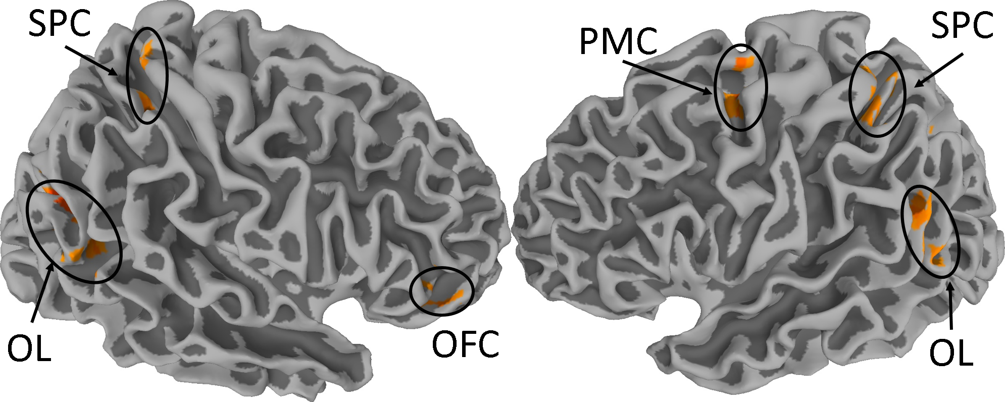
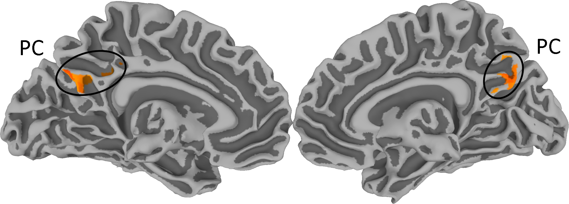
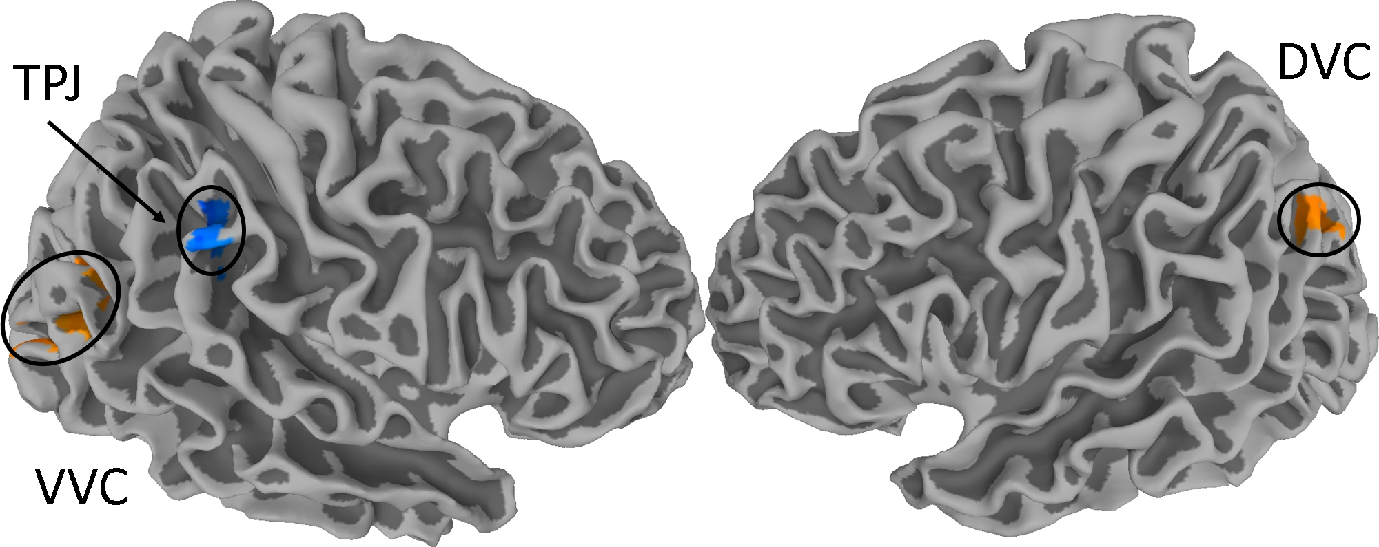
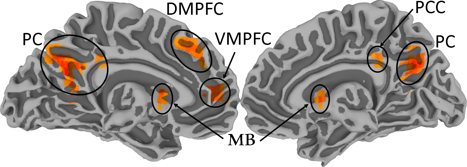
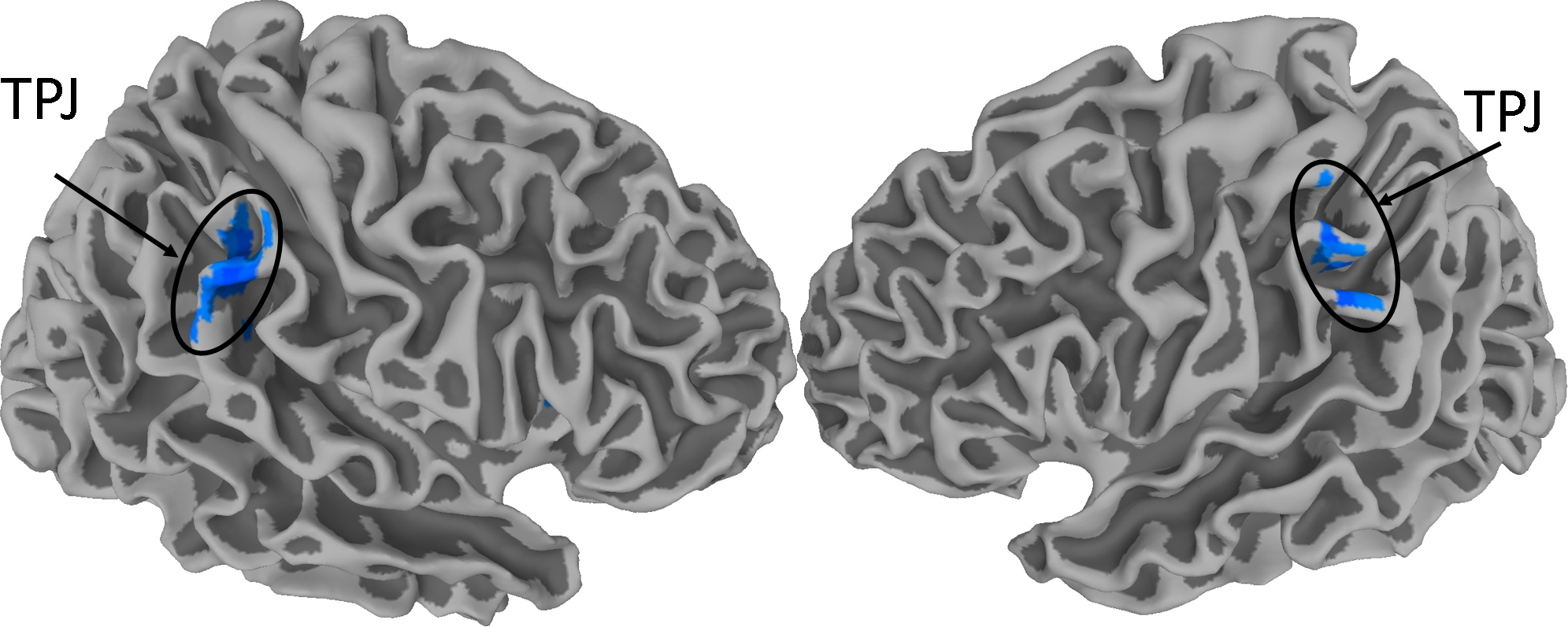
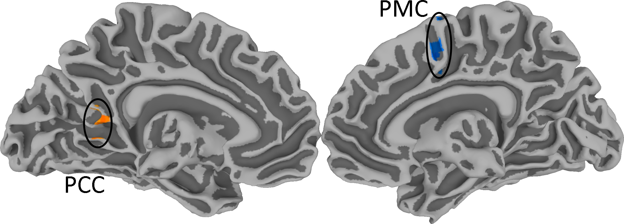
The United States Center for Disease Control and Prevention reports that 47173 Americans died by suicide in 2017, accounting for about two-thirds of all homicides in that year. Accurate suicide risk assessment is challenging, even for trained mental health professionals, as 78% of patients who commit suicide deny such ideation even in their last communication with professionals [6]. Understanding how subjects at risk of suicide respond to different stimuli is important to guide treatment and therapy. [7] provided data from a functional Magnetic Resonance Imaging (fMRI) study of nine suicide attempters and eight suicide non-attempter ideators (henceforth, ideators) upon exposing them to ten words each with positive, negative or death-related connotations. Our interest is in understanding brain regions associated with the interaction of a subject’s attempter/ideator status and word type to inform diagnosis and treatment.

Traditional approaches fit separate regression models at each voxel without regard to spatial context that is only addressed post hoc at the time of inference. A more holistic strategy would use (1) with the response vector 𝒚isubscript𝒚𝑖\bm{y}_{i} of size 30×43×56×20=144480030435620144480030\!\times\!43\!\times\!56\!\times\!20\!=\!1444800, which contains thirty 43×56×2043562043\!\times\!56\!\times\!20 image volumes, for each of the i=1,2,,17𝑖1217i=1,2,\!\hbox to10.00002pt{.\hss.\hss.},17 subjects. The explanatory variable here is a 2D vector that indicates a subject’s status as a suicide attempter or ideator. Under this framework, B𝐵B and ΣΣ\Sigma have over 2.8 million and 1 trillion unconstrained parameters, making estimation with only 171717 subjects impractical. Incorporating a 3D spatial autoregressive (AR) structure into the image volume, and another correlation structure between the words can allow estimation of the variance, but still needs additional methodology to accomodate the large sixth-order tensor-structured regression parameter B𝐵B. We develop such methodology in this paper, and return to this dataset in Section IV-A.

I-A2 Distinguishing characteristics of faces

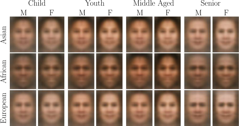
Distinguishing the visual characteristics of faces is important for biometrics. The Labeled Faces in the Wild (LFW) database [8] is used for developing and testing facial recognition methods, and contains over 13000 250×250250250250\times 250 color images of faces of different individuals along with their classification into ethnic origin, age group and gender [9, 10]. We use a subset, totalling 605 images, for which the three attributes of ethnic origin (African, European or Asian, as specified in the database), cohort (child, youth, middle-aged or senior) and gender (male or female) are unambiguous. The color at each pixel is a 3D RGB vector so each image (response) is a 250×250×32502503250\!\times\!250\!\times\!3 array. The three image attributes can each be represented by an indicator vector, so the covariates (attributes) have a three-way tensor-variate structure. Our objective is to train a linear model to help us distinguish the visual characteristics of different attributes. Transforming the 3D tensors into vectors and fitting (1) requires a B𝐵B of 250×250×3×2×3×42502503234250\!\times\!250\!\times\!3\!\times\!2\!\times\!3\!\times\!4 or 4.5 million unconstrained parameters and an error covariance matrix ΣΣ\Sigma of over 17 billion similar parameters, making accurate inference (from only 605 observed images) impractical. Methodology that incorporates the reductions afforded by the tensor-variate structures of the responses and the covariates can redeem the situation. We revisit this dataset in Section IV-B.

I-B Related work and overview of our contributions

The previous examples show the inadequacy of training (1) on tensor-valued data without additional accommodation for structure, as the sizes of B𝐵B and ΣΣ\Sigma in unconstrained vector-variate regression grow with the dimensions of the tensor-valued responses and explanatory variables. Several regression frameworks [11, 12] that efficiently allow for tensor responses [13, 14, 15] or covariates [16, 17, 18, 19, 20, 21, 22, 23, 24, 25, 26, 27, 28] have recently been considered. Tensor-on-tensor regression (ToTR) refers to the case where both the response and covariates are tensors. In this context, [13] proposed an outer matrix product (OP) factorization of B𝐵B, [29] suggested canonical polyadic or CANDECOMP/PARAFAC (CP) decomposition [30, 31], while [32] and [33] factorized B𝐵B using a tensor ring (TR) [34, 35] format. Finally, [36] considered a Tucker (TK) [37, 38, 39] framework but failed to include necessary constraints in their estimation algorithm. The CP, TR and OP formats on B𝐵B allow for quantum dimension reduction without affecting prediction or discrimination ability of the regression model. However, these methodologies do not account for dependence within tensor observations, the sampling distribution of their estimated coefficients and the natural connection that exists between ToTR and the related analysis of variance (ANOVA). Here, we propose a general ToTR framework that renders four low-rank tensor formats on the coefficient B𝐵B: CP, TK, TR and the OP, while simultaneously allowing the errors to follow a tensor-variate normal (TVN) distribution [40, 41, 42, 43] that posits a Kronecker structure on the ΣΣ\Sigma of (1). Assuming TVN-distributed errors allows us to obtain the sampling distributions of the estimated coefficients under their assumed low-rank format. Indeed, Section IV-A uses our derived sampling distributions to produce statistical parametric maps to help detect significant neurological interactions between death-related words and suicide attempter/ideator status. The TVN assumption on the errors also allows us to consider dependence within the tensor-valued observations. The Kronecker structured ΣΣ\Sigma in the TVN model renders a different covariance matrix for each tensor dimension, allowing us to simultaneously study multiple dependence contexts within the same framework. Here we also introduce the notion of tensor-variate ANOVA (TANOVA) under the ToTR framework, which is analogous to ANOVA and multivariate ANOVA (MANOVA) being instances of multiple linear regression (MLR) and MVMLR.

The rest of the paper is structured as follows. Section II first presents notations and network diagrams, low-rank tensor formats, the TVN distribution and our preliminary results that we develop for use in this paper. We formulate ToTR and TANOVA methodology with low-rank tensor formats on the covariates, and TVN errors. We provide algorithms for finding maximum likelihood (ML) estimators and study their properties. Section III evaluates performance of our methods in two simulation scenarios while Section IV applies our methodology to the motivating applications of Sections I-A1 and I-A2. We conclude with some discussion. A supplementary appendix with sections, theorems, lemmas, figures and equations prefixed with “S” is also available.

II Theory and Methods

This section introduces a regression model with TVN errors and tensor-valued responses and covariates. We provide notations and definitions, then introduce our models and develop algorithms for ML estimation under the TK, CP, OP and TR low-rank formats. A special case leads us to TANOVA. We also derive asymptotic properties of our estimators and computational complexity of our algorithms.

II-A Background and preliminary results

We provide a unified treatment of tensor reshapings and contractions by integrating the work of [44], [38], and [45] with our own results that we use later. We use tr(.)\operatorname{tr}(.), (.)(.)^{\prime}, and (.)(.)^{-} to denote the trace, transpose, and pseudo-inverse, Insubscript𝐼𝑛I_{n} for the n×n𝑛𝑛n\!\times\!n identity matrix and tensor-product\otimes for the Kronecker product (Section S1 has additional definitions and illustrations). We define tensors as multi-dimensional arrays of numbers. The total number of modes or sides of a tensor is called its order. We use lower-case letters (i.e. x𝑥x) to specify scalars, bold lower-case italics (i.e. 𝒙𝒙\bm{x}) for vectors, upper-case italics (i.e. X𝑋X) for matrices, and calligraphic scripts (i.e. 𝒳𝒳\mathcal{X}) for higher-order tensors. Random matrices or vectors are denoted using 𝑿𝑿\bm{X} and random tensors by 𝓧𝓧\bm{\mathcal{X}}. We denote the (i1,,ip)thsubscript𝑖1subscript𝑖𝑝𝑡(i_{1},\!\hbox to10.00002pt{.\hss.\hss.},i_{p})th element of a p𝑝pth order tensor 𝒳𝒳\mathcal{X} using 𝒳(i1,,ip)𝒳subscript𝑖1subscript𝑖𝑝\mathcal{X}(i_{1},\!\hbox to10.00002pt{.\hss.\hss.},i_{p}) or 𝒳(𝒊)𝒳𝒊\mathcal{X}(\bm{i}) where 𝒊=[i1,,ip]𝒊superscriptsubscript𝑖1subscript𝑖𝑝\bm{i}=[i_{1},\!\hbox to10.00002pt{.\hss.\hss.},i_{p}]^{\prime}. The vector outer product, with notation \circ, of p𝑝p vectors generates the p𝑝pth-order tensor 𝒳=j=1p𝒙j𝒳superscriptsubscript𝑗1𝑝subscript𝒙𝑗\mathcal{X}=\operatorname*{\circ}_{j=1}^{p}\bm{x}_{j} with (i1,,ip)subscript𝑖1subscript𝑖𝑝(i_{1},\!\hbox to10.00002pt{.\hss.\hss.},i_{p})th element 𝒳(𝒊)=j=1p𝒙j(ij).𝒳𝒊superscriptsubscriptproduct𝑗1𝑝subscript𝒙𝑗subscript𝑖𝑗\mathcal{X}(\bm{i})=\prod_{j=1}^{p}\bm{x}_{j}(i_{j}). Any p𝑝pth-order tensor 𝒳m1××mp𝒳superscriptsubscript𝑚1subscript𝑚𝑝\mathcal{X}\in\mathbb{R}^{m_{1}\times\!\hbox to7.00002pt{.\hss.\hss.}\times m_{p}} (or ×j=1pmjsuperscriptsuperscriptsubscript𝑗1𝑝absentsubscript𝑚𝑗\mathbb{R}^{\times_{j=1}^{p}m_{j}}) can be expressed using the vector outer product as

𝒳=i1=1m1ip=1mp𝒳(i1,,ip)(q=1p𝒆iqmq),𝒳superscriptsubscriptsubscript𝑖11subscript𝑚1superscriptsubscriptsubscript𝑖𝑝1subscript𝑚𝑝𝒳subscript𝑖1subscript𝑖𝑝superscriptsubscript𝑞1𝑝superscriptsubscript𝒆subscript𝑖𝑞subscript𝑚𝑞\mathcal{X}=\sum_{i_{1}=1}^{m_{1}}\!\hbox to10.00002pt{.\hss.\hss.}\sum_{i_{p}=1}^{m_{p}}\mathcal{X}(i_{1},\!\hbox to10.00002pt{.\hss.\hss.},i_{p})\big{(}\operatorname*{\circ}_{q=1}^{p}\bm{e}_{i_{q}}^{m_{q}}\big{)}, (2)

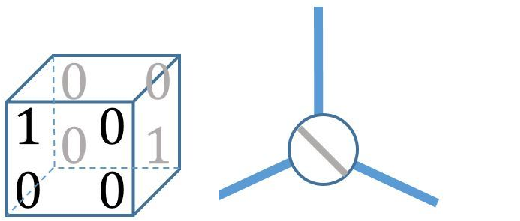
where 𝒆immsuperscriptsubscript𝒆𝑖𝑚superscript𝑚\bm{e}_{i}^{m}\in\mathbb{R}^{m} is a unit basis vector with 1 as the i𝑖ith element and 0 everywhere else. Equation (2) allows us to reshape a tensor by only manipulating the vector outer product. A p𝑝pth-order diagonal tensor 𝕀rp×1prsubscriptsuperscript𝕀𝑝𝑟superscriptsuperscriptsubscript1𝑝absent𝑟\mathbb{I}^{p}_{r}\in\mathbb{R}^{\times_{1}^{p}r} has ones where the indices in each mode coincide, and zeroes elsewhere, that is,

𝕀rp=i=1r(q=1p𝒆ir).subscriptsuperscript𝕀𝑝𝑟superscriptsubscript𝑖1𝑟superscriptsubscript𝑞1𝑝superscriptsubscript𝒆𝑖𝑟\mathbb{I}^{p}_{r}=\sum\limits_{i=1}^{r}(\operatorname*{\circ}\limits_{q=1}^{p}\bm{e}_{i}^{r}). (3)

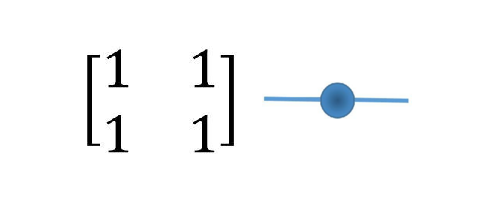
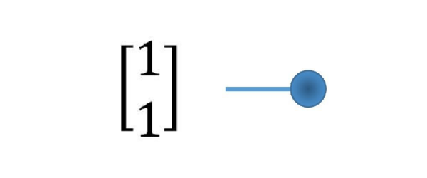
Tensor structures are conveniently represented by tensor network diagrams that are a recent adaptation [45] from quantum physics where they were originally introduced to visually describe many-body problems. Each node in a tensor network diagram corresponds to a tensor and each edge coming from the node represents a mode. A node with no edges is a scalar, a node with one

Refer to caption
(a) x𝑥x\in\mathbb{R}
Refer to caption
(b) 𝒙2𝒙superscript2\bm{x}\in{\mathbb{R}}^{2}
Refer to caption
(c) X2×2𝑋superscript22X\in{\mathbb{R}}^{2\times 2}
Refer to caption
(d) 𝒳2×2×2𝒳superscript222\mathcal{X}\in{\mathbb{R}}^{2\times 2\times 2}
Figure 1: Tensor network diagrams of a (a) scalar, (b) vector, (c) matrix and (d) third-order diagonal tensor.

edge is a vector and a node with two edges is a matrix. More generally, a node with p𝑝p edges is a p𝑝pth-order tensor (Figs. 1a1d). (The angle between edges has no meaning beyond aesthetics.) Diagonal tensors as in (3) are represented by putting a diagonal across the node, as in Fig. 1d.

II-A1 Tensor reshapings, contractions, low-rank formats

The matricization of a tensor is a matrix with its elements arranged differently. The following definition is from [44]

Definition II.1.

Let 𝒮={r1,,rL}𝒮subscript𝑟1subscript𝑟𝐿\mathscr{S}=\{r_{1},\!\hbox to10.00002pt{.\hss.\hss.},r_{L}\} and 𝒯={m1,,mM}𝒯subscript𝑚1subscript𝑚𝑀\mathscr{T}=\{m_{1},\!\hbox to10.00002pt{.\hss.\hss.},m_{M}\} be ordered sets that partition the set of modes ={1,,p}1𝑝\mathscr{M}=\{1,\!\hbox to10.00002pt{.\hss.\hss.},p\} of 𝒳×j=1pmj𝒳superscriptsuperscriptsubscript𝑗1𝑝absentsubscript𝑚𝑗\mathcal{X}\in\mathbb{R}^{\times_{j=1}^{p}m_{j}}. Here L+M=p𝐿𝑀𝑝L+M=p. Then if 𝐢=[i1,,ip]𝐢superscriptsubscript𝑖1subscript𝑖𝑝\bm{i}=[i_{1},\!\hbox to10.00002pt{.\hss.\hss.},i_{p}]^{\prime}, the matricization 𝒳(𝒮×𝒯)subscript𝒳𝒮𝒯\mathcal{X}_{(\mathscr{S}\times\mathscr{T})} is a matrix of size (q𝒮mq)×(q𝒯mq)subscriptproduct𝑞𝒮subscript𝑚𝑞subscriptproduct𝑞𝒯subscript𝑚𝑞(\prod_{q\in\mathscr{S}}m_{q})\times(\prod_{q\in\mathscr{T}}m_{q}) defined as

𝒳(𝒮×𝒯)=i1=1m1ip=1mp𝒳(𝒊)(q𝒮𝒆iqmq)(q𝒯𝒆iqmq).subscript𝒳𝒮𝒯superscriptsubscriptsubscript𝑖11subscript𝑚1superscriptsubscriptsubscript𝑖𝑝1subscript𝑚𝑝𝒳𝒊subscripttensor-product𝑞𝒮superscriptsubscript𝒆subscript𝑖𝑞subscript𝑚𝑞superscriptsubscripttensor-product𝑞𝒯superscriptsubscript𝒆subscript𝑖𝑞subscript𝑚𝑞\mathcal{X}_{(\mathscr{S}\times\mathscr{T})}=\sum\limits_{i_{1}=1}^{m_{1}}\!\hbox to10.00002pt{.\hss.\hss.}\sum\limits_{i_{p}=1}^{m_{p}}\mathcal{X}(\bm{i})\big{(}\bigotimes\limits_{q\in\mathscr{S}}\bm{e}_{i_{q}}^{m_{q}}\big{)}\big{(}\bigotimes\limits_{q\in\mathscr{T}}\bm{e}_{i_{q}}^{m_{q}}\big{)}^{\prime}. (4)

We define matricizations in reverse lexicographic order to be consistent with the traditional matrix vectorization. This means that the q𝑞q modes in the multiple Kronecker product (4) are selected in reverse order.

TABLE I: Tensor reshapings defined by specifying partitions (𝒮,𝒯)𝒮𝒯(\mathscr{S},\mathscr{T}) of \mathscr{M} in (4).
Reshaping Notation 𝒮𝒮\mathscr{S} 𝒯𝒯\mathscr{T}
k𝑘kth mode
matricization
𝒳(k)subscript𝒳𝑘\mathcal{X}_{(k)} {k}𝑘\{k\}
{1,,k1,k+1,\{1,\!\hbox to10.00002pt{.\hss.\hss.},k-1,k+1,
,p}\!\hbox to10.00002pt{.\hss.\hss.},p\}
k𝑘kth canonical
matricization
𝒳<k>subscript𝒳expectation𝑘\mathcal{X}_{<k>} {1,,k}1𝑘\{1,\!\hbox to10.00002pt{.\hss.\hss.},k\} {k+1,,p}𝑘1𝑝\{k+1,\!\hbox to10.00002pt{.\hss.\hss.},p\}
vectorization vec(𝒳)vec𝒳\operatorname{vec}(\mathcal{X}) {1,,p}1𝑝\{1,\!\hbox to10.00002pt{.\hss.\hss.},p\} \varnothing

Table I defines several reshapings by selecting different partitions (𝒮,𝒯)𝒮𝒯(\mathscr{S},\mathscr{T}) of \mathscr{M}. These definitions are clarified in (S3), (S4) and (S5).

Tensor contractions [45] generalize the matrix product to higher-ordered tensors. We use 𝒳×k1,,kal1,,la𝒴superscriptsubscriptsubscript𝑘1subscript𝑘𝑎subscript𝑙1subscript𝑙𝑎𝒳𝒴\mathcal{X}\times_{k_{1},\!\hbox to7.00002pt{.\hss.\hss.},k_{a}}^{l_{1},\!\hbox to7.00002pt{.\hss.\hss.},l_{a}}\mathcal{Y} to denote the mode-(l1,,lak1,,ka)binomialsubscript𝑙1subscript𝑙𝑎subscript𝑘1subscript𝑘𝑎{{l_{1},\!\hbox to10.00002pt{.\hss.\hss.},l_{a}}\choose{k_{1},\!\hbox to7.00002pt{.\hss.\hss.},k_{a}}} product or contraction between the (k1,,ka)subscript𝑘1subscript𝑘𝑎(k_{1},\!\hbox to10.00002pt{.\hss.\hss.},k_{a}) modes of 𝒳×j=1pmj𝒳superscriptsuperscriptsubscript𝑗1𝑝absentsubscript𝑚𝑗\mathcal{X}\in\mathbb{R}^{\times_{j=1}^{p}m_{j}} and the (l1,,la)subscript𝑙1subscript𝑙𝑎(l_{1},\!\hbox to10.00002pt{.\hss.\hss.},l_{a}) modes of 𝒴×j=1qnj𝒴superscriptsuperscriptsubscript𝑗1𝑞absentsubscript𝑛𝑗\mathcal{Y}\in\mathbb{R}^{\times_{j=1}^{q}n_{j}}, where mk1=nl1,,mka=nlaformulae-sequencesubscript𝑚subscript𝑘1subscript𝑛subscript𝑙1subscript𝑚subscript𝑘𝑎subscript𝑛subscript𝑙𝑎m_{k_{1}}=n_{l_{1}},\ldots,m_{k_{a}}=n_{l_{a}}. This contraction results in a tensor of order p+q2a𝑝𝑞2𝑎p+q-2a where the a𝑎a pairs of modes (lj,kj)subscript𝑙𝑗subscript𝑘𝑗(l_{j},k_{j}) get contracted. A simple contraction between the k𝑘kth mode of 𝒳𝒳\mathcal{X} and the l𝑙lth mode of 𝒴𝒴\mathcal{Y} has (i1,,ik1,ik+1,,ip,j1,,jl1,jl+1,,jq)subscript𝑖1subscript𝑖𝑘1subscript𝑖𝑘1subscript𝑖𝑝subscript𝑗1subscript𝑗𝑙1subscript𝑗𝑙1subscript𝑗𝑞(i_{1},\!\hbox to10.00002pt{.\hss.\hss.},i_{k-1},i_{k+1},\!\hbox to10.00002pt{.\hss.\hss.},i_{p},j_{1},\!\hbox to10.00002pt{.\hss.\hss.},j_{l-1},j_{l+1},\!\hbox to10.00002pt{.\hss.\hss.},j_{q})th element

t=1ml𝒳(i1,,ik1,t,ik+1,,ip)𝒴(j1,,jl1,t,jl+1,,jq).superscriptsubscript𝑡1subscript𝑚𝑙𝒳subscript𝑖1subscript𝑖𝑘1𝑡subscript𝑖𝑘1subscript𝑖𝑝𝒴subscript𝑗1subscript𝑗𝑙1𝑡subscript𝑗𝑙1subscript𝑗𝑞\displaystyle\sum\limits_{t=1}^{m_{l}}\mathcal{X}(i_{1},\!\hbox to10.00002pt{.\hss.\hss.},i_{k-1},t,i_{k+1},\!\hbox to10.00002pt{.\hss.\hss.},i_{p})\mathcal{Y}(j_{1},\!\hbox to10.00002pt{.\hss.\hss.},j_{l-1},t,j_{l+1},\!\hbox to10.00002pt{.\hss.\hss.},j_{q}). (5)

Similarly, multiple contractions sum over multiple products of the elements of 𝒳𝒳\mathcal{X} and 𝒴𝒴\mathcal{Y}. Table II defines some contractions using this notation. An important special case is partial contraction that contracts all the p<q𝑝𝑞p<q modes of 𝒳×j=1pmj𝒳superscriptsuperscriptsubscript𝑗1𝑝absentsubscript𝑚𝑗\mathcal{X}\in\mathbb{R}^{\times_{j=1}^{p}m_{j}} with the first p𝑝p modes of 𝒴×j=1qmj𝒴superscriptsuperscriptsubscript𝑗1𝑞absentsubscript𝑚𝑗\mathcal{Y}\in\mathbb{R}^{\times_{j=1}^{q}m_{j}} resulting in a tensor 𝒳|𝒴=𝒳×1,,p1,,p𝒴inner-product𝒳𝒴superscriptsubscript1𝑝1𝑝𝒳𝒴\langle\mathcal{X}|\mathcal{Y}\rangle=\mathcal{X}\times_{1,\!\hbox to7.00002pt{.\hss.\hss.},p}^{1,\!\hbox to7.00002pt{.\hss.\hss.},p}\mathcal{Y} of size ×j=p+1qmj.superscriptsuperscriptsubscript𝑗𝑝1𝑞absentsubscript𝑚𝑗\mathbb{R}^{\times_{j=p+1}^{q}m_{j}}. The partial contraction helps define ToTR, and can also be written as a matrix-vector multiplication using Lemma II.1 (e) (below).

TABLE II: Tensor contractions, where the contraction along one mode is defined as per (5). Here 𝒳×j=1pmj𝒳superscriptsuperscriptsubscript𝑗1𝑝absentsubscript𝑚𝑗\mathcal{X}\in\mathbb{R}^{\times_{j=1}^{p}m_{j}}, 𝒴×j=1qnj𝒴superscriptsuperscriptsubscript𝑗1𝑞absentsubscript𝑛𝑗\mathcal{Y}\in\mathbb{R}^{\times_{j=1}^{q}n_{j}}, and X𝑋X and Y𝑌Y are the cases where p=2𝑝2p=2 and q=2𝑞2q=2 respectively.
Contraction Notation Definition Conditions
matrix product XY𝑋𝑌XY X×21Ysuperscriptsubscript21𝑋𝑌X\times_{2}^{1}Y p=q=2𝑝𝑞2p=q=2
k𝑘kth mode
matrix product
𝒳×kYsubscript𝑘𝒳𝑌\mathcal{X}\times_{k}Y 𝒳×k2Ysuperscriptsubscript𝑘2𝒳𝑌\mathcal{X}\times_{k}^{2}Y q=2𝑞2q=2
k𝑘kth mode
vector product
𝒳ׯk𝒚𝒳subscript¯𝑘𝒚\mathcal{X}\bar{\times}_{k}\bm{y} 𝒳×k1𝒚superscriptsubscript𝑘1𝒳𝒚\mathcal{X}\times_{k}^{1}\bm{y} q=1𝑞1q=1
inner product 𝒳,𝒴𝒳𝒴\langle\mathcal{X},\mathcal{Y}\rangle 𝒳×1,,p1,,q𝒴superscriptsubscript1𝑝1𝑞𝒳𝒴\mathcal{X}\times_{1,\!\hbox to7.00002pt{.\hss.\hss.},p}^{1,\!\hbox to7.00002pt{.\hss.\hss.},q}\mathcal{Y} p=q𝑝𝑞p=q
partial contraction 𝒳|𝒴inner-product𝒳𝒴\langle\mathcal{X}|\mathcal{Y}\rangle 𝒳×1,,p1,,p𝒴superscriptsubscript1𝑝1𝑝𝒳𝒴\mathcal{X}\times_{1,\!\hbox to7.00002pt{.\hss.\hss.},p}^{1,\!\hbox to7.00002pt{.\hss.\hss.},p}\mathcal{Y} p<q𝑝𝑞p<q
last mode with
first mode
𝒳×1𝒴superscript1𝒳𝒴\mathcal{X}\times^{1}\mathcal{Y} 𝒳×p1𝒴superscriptsubscript𝑝1𝒳𝒴\mathcal{X}\times_{p}^{1}\mathcal{Y}

The tensor trace is a self-contraction between the two outer-most modes of a tensor. If m1=mpsubscript𝑚1subscript𝑚𝑝m_{1}=m_{p}, then

tr(𝒳)=i=1m1𝒳(i,:,:,:,i),\operatorname{tr}(\mathcal{X})=\sum_{i=1}^{m_{1}}\mathcal{X}(i,:,:\!\hbox to10.00002pt{.\hss.\hss.},:,i), (6)

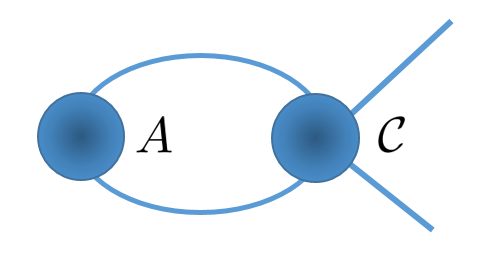
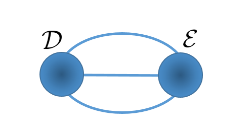
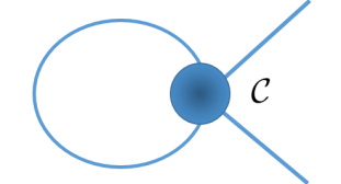
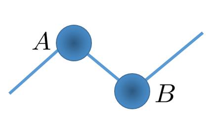
whence tr(𝒳)×j=2p+1mjtr𝒳superscriptsuperscriptsubscript𝑗2𝑝1absentsubscript𝑚𝑗\operatorname{tr}(\mathcal{X})\in\mathbb{R}^{\times_{j=2}^{p+1}m_{j}}. The contraction between two distinct modes (from possibly the same tensor) is represented in tensor network diagrams by joining the corresponding edges (see Fig. 2 for examples).
Refer to caption
(a) ABp×r𝐴𝐵superscript𝑝𝑟AB\!\in\!\mathbb{R}^{p\times r}
Refer to caption
(b) A|𝒞r×sinner-product𝐴𝒞superscript𝑟𝑠\langle A|\mathcal{C}\rangle\!\in\!\mathbb{R}^{r\times s}
Refer to caption
(c) 𝒟,𝒟\langle\mathcal{D},\mathcal{E}\rangle\!\in\!\mathbb{R}
Refer to caption
(d) tr(𝒞)q×rtr𝒞superscript𝑞𝑟\operatorname{tr}(\mathcal{C})\!\in\!\mathbb{R}^{q\times r}
Figure 2: Tensor network diagrams of (a) matrix product, (b) partial contraction, (c) inner product and (d) trace. Here Ap×q𝐴superscript𝑝𝑞A\in\mathbb{R}^{p\times q}, Bq×r𝐵superscript𝑞𝑟B\in\mathbb{R}^{q\times r}, 𝒟,p×q×r𝒟superscript𝑝𝑞𝑟\mathcal{D},\mathcal{E}\in\mathbb{R}^{p\times q\times r} and 𝒞p×q×r×p𝒞superscript𝑝𝑞𝑟𝑝\mathcal{C}\in\mathbb{R}^{p\times q\times r\times p}.

Also, applying the k𝑘kth mode matricization to every mode of 𝒱×j=1pgj𝒱superscriptsuperscriptsubscript𝑗1𝑝absentsubscript𝑔𝑗\mathcal{V}\in\mathbb{R}^{\times_{j=1}^{p}g_{j}} with respect to (WRT) Aimi×gi,i=1,2,,pformulae-sequencesubscript𝐴𝑖superscriptsubscript𝑚𝑖subscript𝑔𝑖𝑖12𝑝A_{i}\in\mathbb{R}^{m_{i}\times g_{i}},i=1,2,\!\hbox to10.00002pt{.\hss.\hss.},p results in the TK product =[[𝒱;A1,,Ap]]delimited-[]𝒱subscript𝐴1subscript𝐴𝑝\mathcal{B}=[\![\mathcal{V};A_{1},\!\hbox to10.00002pt{.\hss.\hss.},A_{p}]\!] defined as

=i1=1m1ip=1mp𝒱(i1ip)(q=1pAq(:,iq)).superscriptsubscriptsubscript𝑖11subscript𝑚1superscriptsubscriptsubscript𝑖𝑝1subscript𝑚𝑝𝒱subscript𝑖1subscript𝑖𝑝superscriptsubscript𝑞1𝑝subscript𝐴𝑞:subscript𝑖𝑞\displaystyle\mathcal{B}=\sum\limits_{i_{1}=1}^{m_{1}}\!\hbox to10.00002pt{.\hss.\hss.}\sum\limits_{i_{p}=1}^{m_{p}}\mathcal{V}{(i_{1}\!\hbox to10.00002pt{.\hss.\hss.}i_{p})}\big{(}\operatorname*{\circ}\limits_{q=1}^{p}A_{q}(:,i_{q})\big{)}. (7)

A tensor \mathcal{B} that can be written as the product in (7) is said to have a TK format with TK rank (g1,,gp)subscript𝑔1subscript𝑔𝑝(g_{1},\!\hbox to10.00002pt{.\hss.\hss.},g_{p}). In this case, 𝒱𝒱\mathcal{V} is called the core tensor and A1,,Apsubscript𝐴1subscript𝐴𝑝A_{1},\!\hbox to10.00002pt{.\hss.\hss.},A_{p} are the factor matrices. When gi<<mimuch-less-thansubscript𝑔𝑖subscript𝑚𝑖g_{i}<<m_{i} for i=1,,p𝑖1𝑝i=1,\ldots,p, the TK format substantially reduces the number of unconstrained elements in a tensor and its complexity. TK formats are often fit by higher-order singular value (HOSVD) [46] or LQ (HOLQ) decomposition [47]. For a diagonal core tensor 𝒱𝒱\mathcal{V}, as in (3), the TK format reduces to the CP format of rank r𝑟r. This reduction is equivalent to setting the tensor \mathcal{B} as the sum of r𝑟r vector outer products, where the vectors correspond to the columns of matrix factors Aimi×r,i=1,,pformulae-sequencesubscript𝐴𝑖superscriptsubscript𝑚𝑖𝑟𝑖1𝑝A_{i}\in\mathbb{R}^{m_{i}\times r},i=1,\ldots,p,

=[[𝝀;A1,,Ap]]=i=1r𝝀(i)(q=1pAq(:,i)).delimited-[]𝝀subscript𝐴1subscript𝐴𝑝superscriptsubscript𝑖1𝑟𝝀𝑖superscriptsubscript𝑞1𝑝subscript𝐴𝑞:𝑖\mathcal{B}=[\![\bm{\lambda};A_{1},\!\hbox to10.00002pt{.\hss.\hss.},A_{p}]\!]=\sum_{i=1}^{r}\bm{\lambda}(i)\big{(}\operatorname*{\circ}\limits_{q=1}^{p}A_{q}(:,i)\big{)}. (8)

The vector 𝝀r𝝀superscript𝑟\bm{\lambda}\in\mathbb{R}^{r} contains the diagonal entries of the core tensor, and is often set to the proportionality constants that make the matrix factors have unit column norms. When 𝝀𝝀\bm{\lambda} is ignored in the specification of (8), we assume that 𝝀=[1,1,,1]𝝀superscript111\bm{\lambda}=[1,1,\!\hbox to10.00002pt{.\hss.\hss.},1]^{\prime}. A tensor \mathcal{B} is said to have an OP format if it can be written as =[[A1,A2,Ap]]\mathcal{B}=\circ[\![A_{1},A_{2}\!\hbox to10.00002pt{.\hss.\hss.},A_{p}]\!], or

=i1,ipj1,jp(q=1pAq[iq,jq]){(q=1p𝒆jqhq)(q=1p𝒆iqmq)},subscriptsubscript𝑖1subscript𝑖𝑝subscript𝑗1subscript𝑗𝑝superscriptsubscriptproduct𝑞1𝑝subscript𝐴𝑞subscript𝑖𝑞subscript𝑗𝑞superscriptsubscript𝑞1𝑝superscriptsubscript𝒆subscript𝑗𝑞subscript𝑞superscriptsubscript𝑞1𝑝superscriptsubscript𝒆subscript𝑖𝑞subscript𝑚𝑞\displaystyle\mathcal{B}=\sum\limits_{\begin{subarray}{c}i_{1},\!\hbox to7.00002pt{.\hss.\hss.}i_{p}\\ j_{1}\!\hbox to7.00002pt{.\hss.\hss.},j_{p}\end{subarray}}(\prod\limits_{q=1}^{p}A_{q}[i_{q},j_{q}])\Big{\{}\big{(}\operatorname*{\circ}\limits_{q=1}^{p}\bm{e}_{j_{q}}^{h_{q}}\big{)}\circ\big{(}\operatorname*{\circ}\limits_{q=1}^{p}\bm{e}_{i_{q}}^{m_{q}}\big{)}\Big{\}}, (9)

where for all q=1,,p𝑞1𝑝q=1,\!\hbox to10.00002pt{.\hss.\hss.},p, we have Aqmq×hqsubscript𝐴𝑞superscriptsubscript𝑚𝑞subscript𝑞A_{q}\in\mathbb{R}^{m_{q}\times h_{q}} and the summation over iqsubscript𝑖𝑞i_{q} is from 1 through mqsubscript𝑚𝑞m_{q}, and that over jqsubscript𝑗𝑞j_{q} is from 1 through hqsubscript𝑞h_{q}. Our novel OP format is essentially the outer product of multiple matrices, and is useful for expressing the TK product of (7) as a partial contraction between 𝒱𝒱\mathcal{V} and [[A1,A2,Ap]]absentdelimited-[]subscript𝐴1subscript𝐴2subscript𝐴𝑝\circ[\![A_{1},A_{2}\!\hbox to10.00002pt{.\hss.\hss.},A_{p}]\!], as we shortly state and prove in Theorem II.1(b). The derivation needs some properties of tensor products and reshapings that we prove first in Lemma II.1, along with several other properties that are useful for tensor manipulations. (Lemma II.1(a),(c) and (d) have been stated without proof in [44], [38], and [45] but we provide proofs here for completeness.)

Lemma II.1.

Let 𝒳×j=1pmj𝒳superscriptsuperscriptsubscript𝑗1𝑝absentsubscript𝑚𝑗\mathcal{X}\in\mathbb{R}^{\times_{j=1}^{p}m_{j}}. Then using the notation of Tables I and II, where k=1,,p𝑘1𝑝k=1,\ldots,p,

  1. (a)

    𝒳<p1>=𝒳(p)subscript𝒳expectation𝑝1superscriptsubscript𝒳𝑝\mathcal{X}_{<p-1>}=\mathcal{X}_{(p)}^{\prime}.

  2. (b)

    vec(𝒳)=vec(𝒳(1))=vec(𝒳<1>)==vec(𝒳<p>).vec𝒳vecsubscript𝒳1vecsubscript𝒳expectation1vecsubscript𝒳expectation𝑝\operatorname{vec}(\mathcal{X})=\operatorname{vec}(\mathcal{X}_{(1)})=\operatorname{vec}(\mathcal{X}_{<1>})=\ldots=\operatorname{vec}{(\mathcal{X}_{<p>}}).

  3. (c)

    𝒳,𝒴=(vec𝒳)(vec𝒴)=tr(𝒳(k)𝒴(k))𝒳𝒴superscriptvec𝒳vec𝒴trsubscript𝒳𝑘superscriptsubscript𝒴𝑘\langle\mathcal{X},\mathcal{Y}\rangle\!=\!(\operatorname{vec}{\mathcal{X})}^{\prime}(\operatorname{vec}{\mathcal{Y})}\!=\!\operatorname{tr}{(\mathcal{X}_{(k)}\mathcal{Y}_{(k)}^{\prime})}, 𝒴×j=1pmj𝒴superscriptsuperscriptsubscript𝑗1𝑝absentsubscript𝑚𝑗\mathcal{Y}\in\mathbb{R}^{\times_{j=1}^{p}m_{j}}.

  4. (d)

    vec[[𝒳;A1,,Ap]]=(i=p1Ai)vec(𝒳)vec𝒳subscript𝐴1subscript𝐴𝑝superscriptsubscripttensor-product𝑖𝑝1subscript𝐴𝑖vec𝒳\operatorname{vec}[\![\mathcal{X};A_{1},\!\hbox to10.00002pt{.\hss.\hss.},A_{p}]\!]=\big{(}\bigotimes_{i=p}^{1}A_{i}\big{)}\operatorname{vec}(\mathcal{X}), where AiRni×misubscript𝐴𝑖superscript𝑅subscript𝑛𝑖subscript𝑚𝑖A_{i}\in R^{n_{i}\times m_{i}} for any nisubscript𝑛𝑖n_{i}\in\mathbb{N}.

  5. (e)

    vec𝒳|=<p>vec𝒳,(×j=1pmj)×(×j=1qhj).formulae-sequencevecinner-product𝒳superscriptsubscriptexpectation𝑝vec𝒳superscriptsuperscriptsubscript𝑗1𝑝absentsubscript𝑚𝑗superscriptsubscript𝑗1𝑞absentsubscript𝑗\operatorname{vec}\langle\mathcal{X}|\mathcal{B}\rangle=\mathcal{B}_{<p>}^{\prime}\operatorname{vec}{\mathcal{X}},\mathcal{B}\in\mathbb{R}^{(\times_{j=1}^{p}m_{j})\times(\times_{j=1}^{q}h_{j})}.

  6. (f)

    vec𝒳(k)=K(k)vec(𝒳),whereK(k)=(Ii=k+1pmiKi=1k1mi,mk).formulae-sequencevecsubscript𝒳𝑘subscript𝐾𝑘vec𝒳𝑤𝑒𝑟𝑒subscript𝐾𝑘tensor-productsubscript𝐼superscriptsubscriptproduct𝑖𝑘1𝑝subscript𝑚𝑖subscript𝐾superscriptsubscriptproduct𝑖1𝑘1subscript𝑚𝑖subscript𝑚𝑘\operatorname{vec}\mathcal{X}_{(k)}=K_{(k)}\operatorname{vec}{(\mathcal{X})},\quad whereK_{(k)}\!=\!\big{(}I_{\prod_{i=k+1}^{p}m_{i}}\otimes K_{\prod_{i=1}^{k-1}m_{i},m_{k}}\big{)}.

Proof.

See Section S1-C. ∎

We now use Lemma II.1 to state and prove the following

Theorem II.1.

Consider a p𝑝pth-order tensor 𝒳𝒳\mathcal{X} and matrices M1,,Mpsubscript𝑀1subscript𝑀𝑝M_{1},\ldots,M_{p} such that the TK product with 𝒳𝒳\mathcal{X} can be formed. Then

  1. (a)

    [[M1,,Mp]]<p>=q=p1Mq\circ[\![M_{1},\ldots,M_{p}]\!]_{<p>}=\bigotimes_{q=p}^{1}M_{q}^{\prime}.

  2. (b)

    𝒳|[[M1,,Mp]]=[[𝒳;M1,,Mp]].\langle\mathcal{X}|\circ[\![M_{1},\ldots,M_{p}]\!]\rangle=[\![\mathcal{X};M_{1},\!\hbox to10.00002pt{.\hss.\hss.},M_{p}]\!].

  3. (c)

    For any k=1,p𝑘1𝑝k=1,\!\hbox to10.00002pt{.\hss.\hss.}p, let 𝒮={k,p+k}𝒮𝑘𝑝𝑘\mathscr{S}=\{k,p+k\}. Then

    [[M1,,Mp]](𝒮×𝒮𝖼)=(vecMk)(vec[[M1,,Mk1,Mk+1,,Mp]]).\begin{split}\circ[\![&M_{1},\ldots,M_{p}]\!]_{(\mathscr{S}\times\mathscr{S}^{\mathsf{c}})}\\ &=(\operatorname{vec}M_{k}^{\prime})(\operatorname{vec}\circ[\![M_{1},\ldots,M_{k-1},M_{k+1},\ldots,M_{p}]\!])^{\prime}.\end{split} (10)
Proof.

See Section S1-D. ∎

Remark: If =[[X,X]]\mathcal{B}=\circ[\![X^{\prime},X^{\prime}]\!] for some matrix X𝑋X, then Theorem II.1(a) implies that <2>=XXsubscriptexpectation2tensor-product𝑋𝑋\mathcal{B}_{<2>}=X\otimes X while (1,3)×(2,4)=(vecX)(vecX)subscript1324vec𝑋superscriptvec𝑋\mathcal{B}_{(1,3)\times(2,4)}=(\operatorname{vec}X)(\operatorname{vec}X)^{\prime} by Theorem II.1(c). In other words, XXtensor-product𝑋𝑋X\otimes X and (vecX)(vecX)vec𝑋superscriptvec𝑋(\operatorname{vec}X)(\operatorname{vec}X)^{\prime} are different matricizations of the same OP tensor \mathcal{B}, which formalizes our intuition because both XXtensor-product𝑋𝑋X\otimes X and (vecX)(vecX)vec𝑋superscriptvec𝑋(\operatorname{vec}X)(\operatorname{vec}X)^{\prime} have the same number of elements, and it motivates naming the format outer product.

Finally, a tensor \mathcal{B} is said to have a Tensor Ring (TR) format with TR rank (g1,,gp)subscript𝑔1subscript𝑔𝑝(g_{1},\!\hbox to10.00002pt{.\hss.\hss.},g_{p}) if it can be expressed as

=tr(𝒢1×1×1𝒢p),trsuperscript1superscript1subscript𝒢1subscript𝒢𝑝\mathcal{B}=\operatorname{tr}(\mathcal{G}_{1}\times^{1}\!\hbox to10.00002pt{.\hss.\hss.}\times^{1}\mathcal{G}_{p}), (11)

where 𝒢igi1×mi×gisubscript𝒢𝑖superscriptsubscript𝑔𝑖1subscript𝑚𝑖subscript𝑔𝑖\mathcal{G}_{i}\in\mathbb{R}^{g_{i-1}\times m_{i}\times g_{i}} for i=1,,p𝑖1𝑝i=1,\!\hbox to10.00002pt{.\hss.\hss.},p and g0=gpsubscript𝑔0subscript𝑔𝑝g_{0}=g_{p}. The TR format is called the Matrix Product State (MPS) with closed boundary conditions in many-body physics [48]. When exactly one of the TR ranks is 1, the TR format is the same as the Tensor Train (TT) format [35] and is the MPS with open boundary conditions.

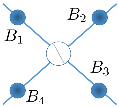
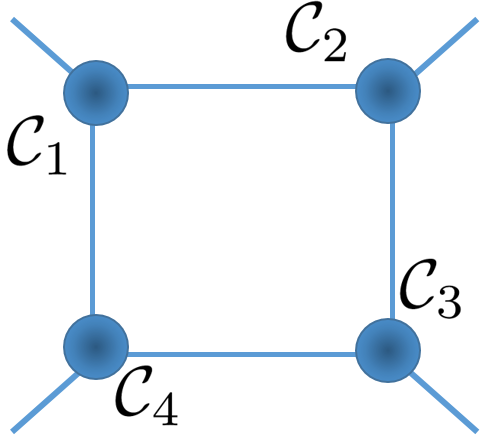
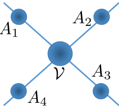
We conclude our discussion of low-rank tensor formats by using tensor network diagrams to illustrate in Fig. 3, a fourth-order tensor in the TK, CP and TR formats.
Refer to caption
(a) [[𝒱;A1,A2,A3,A4]]delimited-[]𝒱subscript𝐴1subscript𝐴2subscript𝐴3subscript𝐴4[\![\mathcal{V};A_{1},A_{2},A_{3},A_{4}]\!]
Refer to caption
(b) [[B1,B2,B3,B4]]delimited-[]subscript𝐵1subscript𝐵2subscript𝐵3subscript𝐵4[\![B_{1},B_{2},B_{3},B_{4}]\!]
Refer to caption
(c) tr(𝒞1×1𝒞2×1𝒞3×1𝒞4)trsuperscript1superscript1superscript1subscript𝒞1subscript𝒞2subscript𝒞3subscript𝒞4\operatorname{tr}(\mathcal{C}_{1}\!\times^{1}\!\mathcal{C}_{2}\!\times^{1}\!\mathcal{C}_{3}\!\times^{1}\!\mathcal{C}_{4})
Figure 3: Tensor network diagrams of example fourth-order tensor of (a) TK format (7), (b) CP format (8), and (c) TR format (11).

II-A2 The TVN Distribution

The matrix-variate normal distribution, abbreviated in [49] as MxVN to distinguish it from the vector-variate multinormal distribution (MVN), was studied extensively in [50]. A random matrix 𝑿m1×m2𝑿superscriptsubscript𝑚1subscript𝑚2\bm{X}\in\mathbb{R}^{m_{1}\times m_{2}} follows a MxVN distribution if vec(𝑿)vec𝑿\operatorname{vec}(\bm{X}) is MVN with covariance matrix Σ2Σ1tensor-productsubscriptΣ2subscriptΣ1\Sigma_{2}\otimes\Sigma_{1}, where Σkmk×mksubscriptΣ𝑘superscriptsubscript𝑚𝑘subscript𝑚𝑘\Sigma_{k}\in\mathbb{R}^{m_{k}\times m_{k}} for k=1,2𝑘12k=1,2. Our TVN distribution, formulated in Definition II.2, extends this idea to the case of higher-order random tensors. For simplicity, we define the following notation for use in the rest of the paper:

m=i=1pmi,mk=m/mk,Σ=i=p1Σi,Σk=i=pik1Σi.formulae-sequence𝑚superscriptsubscriptproduct𝑖1𝑝subscript𝑚𝑖formulae-sequencesubscript𝑚𝑘𝑚subscript𝑚𝑘formulae-sequenceΣsuperscriptsubscripttensor-product𝑖𝑝1subscriptΣ𝑖subscriptΣ𝑘superscriptsubscripttensor-product𝑖𝑝𝑖𝑘1subscriptΣ𝑖m=\prod_{i=1}^{p}m_{i},\hskip 2.84544ptm_{-k}=m/m_{k},\hskip 2.84544pt\Sigma=\bigotimes_{i=p}^{1}\Sigma_{i},\hskip 2.84544pt\Sigma_{-k}=\bigotimes_{\begin{subarray}{c}i=p\\ i\neq k\end{subarray}}^{1}\Sigma_{i}.
Definition II.2.

A random tensor 𝓧×j=1pmj𝓧superscriptsuperscriptsubscript𝑗1𝑝absentsubscript𝑚𝑗\bm{\mathcal{X}}\in\mathbb{R}^{\times_{j=1}^{p}m_{j}} follows a p𝑝pth-order TVN distribution with mean ×j=1pmjsuperscriptsuperscriptsubscript𝑗1𝑝absentsubscript𝑚𝑗\mathcal{M}\in\mathbb{R}^{\times_{j=1}^{p}m_{j}} and non-negative definite scale matrices Σimi×misubscriptΣ𝑖superscriptsubscript𝑚𝑖subscript𝑚𝑖\Sigma_{i}\in\mathbb{R}^{m_{i}\times m_{i}} for i=1,2,,p𝑖12𝑝i=1,2,\ldots,p (i.e., 𝓧𝒩𝐦(,Σ1,Σ2,Σp)similar-to𝓧subscript𝒩𝐦subscriptΣ1subscriptΣ2subscriptΣ𝑝\bm{\mathcal{X}}\sim\operatorname{\mathcal{N}}_{\bm{m}}\big{(}\mathcal{M},\Sigma_{1},\Sigma_{2}\ldots,\Sigma_{p}\big{)} where 𝐦=[m1,m2,,mp]𝐦superscriptsubscript𝑚1subscript𝑚2subscript𝑚𝑝\bm{m}=[m_{1},m_{2},\ldots,m_{p}]^{\prime} ) if vec(𝓧)𝒩m(vec(),Σ).similar-tovec𝓧subscript𝒩𝑚vecΣ\operatorname{vec}(\bm{\mathcal{X}})\sim\operatorname{\mathcal{N}}_{m}\big{(}\operatorname{vec}(\mathcal{M}),\Sigma\big{)}.

The Kronecker product in Definition II.2 is in reverse order because we have defined vectorization in reverse lexicographic order. Definition II.2 defines the TVN distribution in terms of a vectorization. We state and prove the distribution of other tensor reshapings in Theorem II.2. These results are essential in the development of ToTR models with TVN errors, as they allow us to model the vectorized tensor errors in terms of the MVN distribution.

Theorem II.2.

The following statements are equivalent:

  1. (a)

    𝓨𝒩𝒎(,Σ1,Σ2,,Σp)similar-to𝓨subscript𝒩𝒎subscriptΣ1subscriptΣ2subscriptΣ𝑝\bm{\mathcal{Y}}\sim\operatorname{\mathcal{N}}_{\bm{m}}(\mathcal{M},\Sigma_{1},\Sigma_{2},\!\hbox to10.00002pt{.\hss.\hss.},\Sigma_{p})

  2. (b)

    vec(𝓨)𝒩m(vec(),Σ)similar-tovec𝓨subscript𝒩𝑚vecΣ\operatorname{vec}(\bm{\mathcal{Y}})\sim\operatorname{\mathcal{N}}_{m}(\operatorname{vec}(\mathcal{M}),\Sigma)

  3. (c)

    𝓨(k)𝒩[mk,mk]((k),Σk,Σk),k=1,2,,pformulae-sequencesimilar-tosubscript𝓨𝑘subscript𝒩superscriptsubscript𝑚𝑘subscript𝑚𝑘subscript𝑘subscriptΣ𝑘subscriptΣ𝑘𝑘12𝑝\bm{\mathcal{Y}}_{(k)}\sim\operatorname{\mathcal{N}}_{[m_{k},m_{-k}]^{\prime}}(\mathcal{M}_{(k)},\Sigma_{k},\Sigma_{-k}),\quad k=1,2,\!\hbox to10.00002pt{.\hss.\hss.},p

  4. (d)

    For k=1,2,,p𝑘12𝑝k=1,2,\ldots,p and 𝒎k=[i=1kmi,i=k+1pmi]subscript𝒎𝑘superscriptsuperscriptsubscriptproduct𝑖1𝑘subscript𝑚𝑖superscriptsubscriptproduct𝑖𝑘1𝑝subscript𝑚𝑖\bm{m}_{k}=[\prod_{i=1}^{k}m_{i},\prod_{i=k+1}^{p}m_{i}]^{\prime},

    𝓨<k>𝒩𝒎k(<k>,i=k1Σi,i=pk+1Σi)similar-tosubscript𝓨expectation𝑘subscript𝒩subscript𝒎𝑘subscriptexpectation𝑘superscriptsubscripttensor-product𝑖𝑘1subscriptΣ𝑖superscriptsubscripttensor-product𝑖𝑝𝑘1subscriptΣ𝑖\bm{\mathcal{Y}}_{<k>}\sim\operatorname{\mathcal{N}}_{\bm{m}_{k}}(\mathcal{M}_{<k>},\bigotimes_{i=k}^{1}\Sigma_{i},\bigotimes_{i=p}^{k+1}\Sigma_{i})

Proof.

(a) and (b) are equivalent, following Definition II.2 while (b) and (c) are so from Lemma II.1(f) with K(k)ΣK(k)=ΣkΣksubscript𝐾𝑘Σsuperscriptsubscript𝐾𝑘tensor-productsubscriptΣ𝑘subscriptΣ𝑘K_{(k)}\Sigma K_{(k)}^{\prime}=\Sigma_{-k}\otimes\Sigma_{k}. Further, (b) and (d) are equivalent because of Lemma II.1(b). ∎

The density of 𝓨𝒩𝒎(,Σ1,Σ2,,Σp)similar-to𝓨subscript𝒩𝒎subscriptΣ1subscriptΣ2subscriptΣ𝑝\bm{\mathcal{Y}}\sim\operatorname{\mathcal{N}}_{\bm{m}}(\mathcal{M},\Sigma_{1},\Sigma_{2},\!\hbox to10.00002pt{.\hss.\hss.},\Sigma_{p}) is f(𝒴;,Σ)=|2πΣ|1/2exp{12DΣ2(𝒴,)},𝑓𝒴Σsuperscript2𝜋Σ1212superscriptsubscript𝐷Σ2𝒴f(\mathcal{Y};\mathcal{M},\Sigma)=|2\pi\Sigma|^{-1/2}\exp\Big{\{}-\frac{1}{2}D_{\Sigma}^{2}(\mathcal{Y},\mathcal{M})\Big{\}}, where DΣ2(𝒴,)superscriptsubscript𝐷Σ2𝒴D_{\Sigma}^{2}(\mathcal{Y},\mathcal{M}) is the squared Mahalanobis distance between 𝒴𝒴\mathcal{Y} and \mathcal{M}, and has the equivalent representation

DΣ2(𝒴,)=vec(𝒴)Σ1vec(𝒴)(𝒴),[[(𝒴);Σ11,Σ21,,Σp1]],\displaystyle\begin{split}D_{\Sigma}^{2}(\mathcal{Y},\mathcal{M})&=\operatorname{vec}(\mathcal{Y}-\mathcal{M})^{\prime}\Sigma^{-1}\operatorname{vec}(\mathcal{Y}-\mathcal{M})\\ &\equiv\langle(\mathcal{Y}-\mathcal{M}),[\![(\mathcal{Y}-\mathcal{M});\Sigma_{1}^{-1},\Sigma_{2}^{-1},\!\hbox to10.00002pt{.\hss.\hss.},\Sigma_{p}^{-1}]\!]\rangle,\end{split} (12)

by Lemmas II.1(c) and II.1(d). Property S1.2 provides similar alternative expressions for the determinant det(Σ)Σ\det{(\Sigma)} of ΣΣ\Sigma.

II-B Tensor-variate Linear Models with TVN Errors

II-B1 Tensor-on-Tensor Regression

We formulate the ToTR model as

𝓨i=Υ+𝒳i|+𝓔i,i=1,2,n,formulae-sequencesubscript𝓨𝑖Υinner-productsubscript𝒳𝑖subscript𝓔𝑖𝑖12𝑛\bm{\mathcal{Y}}_{i}=\Upsilon+\langle\mathcal{X}_{i}|\mathcal{B}\rangle+\bm{\mathcal{E}}_{i},\quad i=1,2\!\hbox to10.00002pt{.\hss.\hss.},n, (13)

where the response 𝓨i×j=1pmjsubscript𝓨𝑖superscriptsuperscriptsubscript𝑗1𝑝absentsubscript𝑚𝑗\bm{\mathcal{Y}}_{i}\!\in\!\mathbb{R}^{\times_{j=1}^{p}m_{j}} and the covariate 𝒳i×j=1lhjsubscript𝒳𝑖superscriptsuperscriptsubscript𝑗1𝑙absentsubscript𝑗\mathcal{X}_{i}\in\mathbb{R}^{\times_{j=1}^{l}h_{j}} are both tensor-valued, 𝓔iiid𝒩𝒎(0,σ2Σ1,Σ2,,Σp)subscript𝓔𝑖𝑖𝑖𝑑similar-tosubscript𝒩𝒎0superscript𝜎2subscriptΣ1subscriptΣ2subscriptΣ𝑝\bm{\mathcal{E}}_{i}\overset{iid}{\sim}\operatorname{\mathcal{N}}_{\bm{m}}(0,\sigma^{2}\Sigma_{1},\Sigma_{2},\ldots,\Sigma_{p}) is the TVN-distributed error, (×j=1lhj)×(×j=1pmj)superscriptsuperscriptsubscript𝑗1𝑙absentsubscript𝑗superscriptsubscript𝑗1𝑝absentsubscript𝑚𝑗\mathcal{B}\in\mathbb{R}^{(\times_{j=1}^{l}h_{j})\times(\times_{j=1}^{p}m_{j})} is the (tensor-valued) regression parameter and ΥΥ\Upsilon is the (tensor-valued) intercept. This model is essentially the classical MVMLR model but exploits the tensor-variate structure of the covariates and responses to reduce the total number of parameters. To see this, we apply Lemma II.1(e) and Theorem II.2(b) to vectorize (13) as vec(𝓨i)=vec(Υ)+<l>vec(𝒳i)+𝒆i,vecsubscript𝓨𝑖vecΥsuperscriptsubscriptexpectation𝑙vecsubscript𝒳𝑖subscript𝒆𝑖\operatorname{vec}(\bm{\mathcal{Y}}_{i})=\operatorname{vec}(\Upsilon)+\mathcal{B}_{<l>}^{\prime}\operatorname{vec}(\mathcal{X}_{i})+\bm{e}_{i}, where 𝒆iiid𝒩m(0,σ2Σ)subscript𝒆𝑖𝑖𝑖𝑑similar-tosubscript𝒩𝑚0superscript𝜎2Σ\bm{e}_{i}\overset{iid}{\sim}\operatorname{\mathcal{N}}_{m}(0,\sigma^{2}\Sigma) is the error. This formulation leads to a MVMLR model with intercept, which can be incorporated into the covariates as [vec(Υ)<l>][1,vec(𝒳i)][\operatorname{vec}(\Upsilon)\mathcal{B}_{<l>}^{\prime}][1,\operatorname{vec}(\mathcal{X}_{i})^{\prime}]^{\prime}. But the covariate [1,vec(𝒳i)][1,\operatorname{vec}(\mathcal{X}_{i})^{\prime}]^{\prime} is then no longer a vectorized tensor and we can not exploit the tensor structure of 𝒳isubscript𝒳𝑖\mathcal{X}_{i}. To obviate this possibility, (13) includes a separate intercept term ΥΥ\Upsilon.

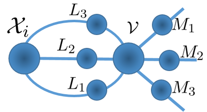
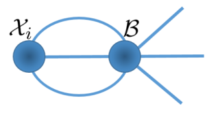
Imposing a low-rank format on \mathcal{B} proffers several advantages. First, it makes the regression model practical to use, as accurate estimation of an unstructured version of \mathcal{B} may otherwise be prohibitive when dimensionality is high relative to sample size. Second, \mathcal{B} can be interpreted, in spite of its high dimensions, as being explainable through a few lower-dimensional tensor factor matrices (Fig. 4).
Refer to caption
(a)
Refer to caption
(b)
Refer to caption
(c)
Refer to caption
(d)
Figure 4: Tensor network diagrams of tensor-on-tensor regression when both the response and the covariates are third-order tensors and for (a) 𝒴i=𝒳i|subscript𝒴𝑖inner-productsubscript𝒳𝑖\mathcal{Y}_{i}=\langle\mathcal{X}_{i}|\mathcal{B}\rangle and (b-d) the special cases when the \mathcal{B} in 𝒳i|inner-productsubscript𝒳𝑖\langle\mathcal{X}_{i}|\mathcal{B}\rangle are of (b) Tucker, (c) TR and (d) OP formats (illustrated in Fig. 3).

These explanations mirror the many-body problem in physics, where weakly-coupled degrees of freedom are often embedded in ultra-high-dimensional Hilbert spaces [48, 51]. We now turn to the problem of learning \mathcal{B} in the given setup.

The dispersion matrix ΣΣ\Sigma in the TVN distribution specification of the 𝓔isubscript𝓔𝑖\bm{\mathcal{E}}_{i}s in (13) is Kronecker-separable and leads to the number of unconstrained parameters from (i=1pmi)×(i=1pmi+1)/2superscriptsubscriptproduct𝑖1𝑝subscript𝑚𝑖superscriptsubscriptproduct𝑖1𝑝subscript𝑚𝑖12(\prod_{i=1}^{p}m_{i})\times(\prod_{i=1}^{p}m_{i}+1)/2 to i=1pmi(mi+1)/2superscriptsubscript𝑖1𝑝subscript𝑚𝑖subscript𝑚𝑖12\sum_{i=1}^{p}m_{i}(m_{i}+1)/2. Further, this Kronecker-separable structure is intuitive because it assigns a covariance matrix to each tensor-response dimension. This allows us to separately incorporate different dependence contexts that exist within a tensor. For example, a tensor may have temporal and spatial contexts in its modes. Kronecker separability allows us to assign a covariance matrix to each of these different contexts. However, Kronecker separability results in unidentifiable scale matrices (Σi)subscriptΣ𝑖(\Sigma_{i}), as cAB=AcBtensor-product𝑐𝐴𝐵tensor-product𝐴𝑐𝐵cA\otimes B=A\otimes cB for any matrices A,B𝐴𝐵A,B and c0𝑐0c\neq 0, so we constrain the scale matrices to each have Σi(1,1)=1subscriptΣ𝑖111\Sigma_{i}(1,1)=1, and introduce a parameter σ2superscript𝜎2\sigma^{2} to capture an overall proportional scalar variance. This approach further reduces the number of parameters by p1𝑝1p-1 and imposes a curved exponential family distribution on the errors [52].

II-B2 The TANOVA model

Suppose that we observe independent tensors 𝓨j1,,jl,i×j=1pmjsubscript𝓨subscript𝑗1subscript𝑗𝑙𝑖superscriptsuperscriptsubscript𝑗1𝑝absentsubscript𝑚𝑗\bm{\mathcal{Y}}_{j_{1},\!\hbox to7.00002pt{.\hss.\hss.},j_{l},i}\in\mathbb{R}^{\times_{j=1}^{p}m_{j}} (i=1,,nj1,,jl)𝑖1subscript𝑛subscript𝑗1subscript𝑗𝑙(i=1,\ldots,n_{j_{1},\ldots,j_{l}}), where jksubscript𝑗𝑘j_{k} (k=1,,l)𝑘1𝑙(k=1,\!\hbox to10.00002pt{.\hss.\hss.},l), indexes the k𝑘kth categorical (factor) variable of hksubscript𝑘h_{k} levels, that is, jk{1,,hk}subscript𝑗𝑘1subscript𝑘j_{k}\in\{1,\!\hbox to10.00002pt{.\hss.\hss.},h_{k}\}. The tensor-valued parameter \mathcal{B} encoding the dimensions of 𝓨i,j1,,jlsubscript𝓨𝑖subscript𝑗1subscript𝑗𝑙\bm{\mathcal{Y}}_{i,j_{1},\!\hbox to7.00002pt{.\hss.\hss.},j_{l}} and all the possible factor classes is of size h1××hl×m1××mpsubscript1subscript𝑙subscript𝑚1subscript𝑚𝑝h_{1}\times\!\hbox to10.00002pt{.\hss.\hss.}\times h_{l}\times m_{1}\times\!\hbox to10.00002pt{.\hss.\hss.}\times m_{p}. To see this, consider the l𝑙lth ordered single-entry tensor 𝒳j1,,jl=q=1l𝒆iqhqsubscript𝒳subscript𝑗1subscript𝑗𝑙superscriptsubscript𝑞1𝑙superscriptsubscript𝒆subscript𝑖𝑞subscript𝑞\mathcal{X}_{j_{1},\!\hbox to7.00002pt{.\hss.\hss.},j_{l}}=\operatorname*{\circ}_{q=1}^{l}\bm{e}_{i_{q}}^{h_{q}} that is unity at (j1,,jl)subscript𝑗1subscript𝑗𝑙(j_{1},\!\hbox to10.00002pt{.\hss.\hss.},j_{l}) and zero everywhere else. Then 𝒳j1,,jl|×j=1pmjinner-productsubscript𝒳subscript𝑗1subscript𝑗𝑙superscriptsuperscriptsubscript𝑗1𝑝absentsubscript𝑚𝑗\langle\mathcal{X}_{j_{1},\!\hbox to7.00002pt{.\hss.\hss.},j_{l}}|\mathcal{B}\rangle\in\mathbb{R}^{\times_{j=1}^{p}m_{j}} and

𝒳j1,,jl|=[j1,,jl,:,:,,:].inner-productsubscript𝒳subscript𝑗1subscript𝑗𝑙subscript𝑗1subscript𝑗𝑙:::\langle\mathcal{X}_{j_{1},\!\hbox to7.00002pt{.\hss.\hss.},j_{l}}|\mathcal{B}\rangle=\mathcal{B}[j_{1},\!\hbox to10.00002pt{.\hss.\hss.},j_{l},:,:,\!\hbox to10.00002pt{.\hss.\hss.},:]. (14)

Therefore, modeling 𝔼(𝓨i,j1,,jl)𝔼subscript𝓨𝑖subscript𝑗1subscript𝑗𝑙\mathbb{E}(\bm{\mathcal{Y}}_{i,j_{1},\!\hbox to7.00002pt{.\hss.\hss.},j_{l}}) as 𝒳j1,,jl|inner-productsubscript𝒳subscript𝑗1subscript𝑗𝑙\langle\mathcal{X}_{j_{1},\!\hbox to7.00002pt{.\hss.\hss.},j_{l}}|\mathcal{B}\rangle results in each factor combination (j1,,jp)subscript𝑗1subscript𝑗𝑝(j_{1},\!\hbox to10.00002pt{.\hss.\hss.},j_{p}) getting assigned its own mean parameter as a sub-tensor of \mathcal{B}. This high-dimensional parameter \mathcal{B} is identical to cell-means MANOVA if we vectorize (14) using Lemma II.1(e) as <l>vec(𝒳j1,,jl)=vec([j1,,jp,:,:,,:]),subscriptsuperscriptexpectation𝑙vecsubscript𝒳subscript𝑗1subscript𝑗𝑙vecsubscript𝑗1subscript𝑗𝑝:::\mathcal{B}^{\prime}_{<l>}\operatorname{vec}(\mathcal{X}_{j_{1},\!\hbox to7.00002pt{.\hss.\hss.},j_{l}})=\operatorname{vec}(\mathcal{B}[j_{1},\!\hbox to10.00002pt{.\hss.\hss.},j_{p},:,:,\!\hbox to10.00002pt{.\hss.\hss.},:]), in which case vec(𝒳j1,,jp)=q=l1𝒆iqhq\operatorname{vec}(\mathcal{X}_{j_{1},\!\hbox to7.00002pt{.\hss.\hss.},j_{p}})=\otimes_{q=l}^{1}\bm{e}_{i_{q}}^{h_{q}} corresponds to a row in the MANOVA design matrix. Although this formulation is fundamentally the same as (14), the latter helps us visualize and formulate a low-rank format on \mathcal{B}. Based on the format, we refer to tensor-valued response regression models with the mean in (14) as TANOVA(l,p)𝑙𝑝(l,p), where l𝑙l is the number of different factors and p𝑝p is the order of the tensor-valued response. In this way, because scalar and vector variables are tensors of order 0 and 1, ANOVA and MANOVA correspond to TANOVA(1,0)10(1,0) and TANOVA(1,1)11(1,1), respectively. In general, TANOVA(l,p)𝑙𝑝(l,p) with TVN errors can be expressed as

𝓨i=𝒳i|+𝓔i,𝓔iiid𝒩𝒎(0,σ2Σ1,Σ2,,Σp),subscript𝓨𝑖inner-productsubscript𝒳𝑖subscript𝓔𝑖subscript𝓔𝑖𝑖𝑖𝑑similar-tosubscript𝒩𝒎0superscript𝜎2subscriptΣ1subscriptΣ2subscriptΣ𝑝\bm{\mathcal{Y}}_{i}=\langle\mathcal{X}_{i}|\mathcal{B}\rangle+\bm{\mathcal{E}}_{i},\quad\bm{\mathcal{E}}_{i}\overset{iid}{\sim}\operatorname{\mathcal{N}}_{\bm{m}}(0,\sigma^{2}\Sigma_{1},\Sigma_{2},\!\hbox to10.00002pt{.\hss.\hss.},\Sigma_{p}), (15)

where 𝒳isubscript𝒳𝑖\mathcal{X}_{i} is the single-entry tensor that contains all the assigned factors of 𝓨isubscript𝓨𝑖\bm{\mathcal{Y}}_{i}, for i=1,,n𝑖1𝑛i=1,\ldots,n. Model (15) is a ToTR model as in (13) with no intercept. This is analogous to ANOVA and MANOVA being special cases of univariate and multivariate multiple linear regressions, respectively. Further, the log-likelihood function of (15) is

=n2log|2πσ2Σ|12σ2i=1nDΣ2(𝓨i,𝒳i|).𝑛22𝜋superscript𝜎2Σ12superscript𝜎2superscriptsubscript𝑖1𝑛superscriptsubscript𝐷Σ2subscript𝓨𝑖inner-productsubscript𝒳𝑖\ell=-\dfrac{n}{2}\log|2\pi\sigma^{2}\Sigma|-\dfrac{1}{2\sigma^{2}}\sum_{i=1}^{n}D_{\Sigma}^{2}(\bm{\mathcal{Y}}_{i},\langle\mathcal{X}_{i}|\mathcal{B}\rangle). (16)

II-C Parameter Estimation

We obtain estimators of (13) before deriving their properties.

II-C1 Profiling the intercept

We first show that the intercept in (13) can be profiled out by centering the covariates and the responses. To see this, we express the loglikelihood in terms of ΥΥ\Upsilon as

=12σ2i=1nDΣ2(𝓨i,Υ+𝒳i|).12superscript𝜎2superscriptsubscript𝑖1𝑛superscriptsubscript𝐷Σ2subscript𝓨𝑖Υinner-productsubscript𝒳𝑖\ell=-\dfrac{1}{2\sigma^{2}}\sum_{i=1}^{n}D_{\Sigma}^{2}(\bm{\mathcal{Y}}_{i},\Upsilon+\langle\mathcal{X}_{i}|\mathcal{B}\rangle). (17)

We define the tensor differential of an inner product WRT ΥΥ\Upsilon using the matrix differential Υ,𝒮=tr(Υ(1)𝒮(1))Υ𝒮trsubscriptΥ1superscriptsubscript𝒮1\langle\partial\Upsilon,\mathcal{S}\rangle=\operatorname{tr}(\partial\Upsilon_{(1)}\mathcal{S}_{(1)}^{\prime}). Applying it to (17) yields

(Υ)=1σ2Υ,[[𝓢;Σ11,,Σp1]],Υ1superscript𝜎2Υdelimited-[]𝓢superscriptsubscriptΣ11superscriptsubscriptΣ𝑝1\partial\ell(\Upsilon)=\dfrac{1}{\sigma^{2}}\langle\partial\Upsilon,[\![\bm{\mathcal{S}};\Sigma_{1}^{-1},\!\hbox to10.00002pt{.\hss.\hss.},\Sigma_{p}^{-1}]\!]\rangle,

where n1𝓢=𝓨¯𝒳¯|Υsuperscript𝑛1𝓢bold-¯𝓨inner-product¯𝒳Υn^{-1}\bm{\mathcal{S}}\!=\!\bm{\mathcal{\bar{Y}}}\!-\!\langle\mathcal{\bar{X}}|\mathcal{B}\rangle\!-\!\Upsilon and 𝓨¯,𝒳¯bold-¯𝓨¯𝒳\bm{\mathcal{\bar{Y}}},\mathcal{\bar{X}} are the averaged responses and covariates. Now, (Υ)=0Υ0\partial\ell(\Upsilon)\!=\!0 if 𝓢=0𝓢0\bm{\mathcal{S}}\!=\!0, and after profiling on \mathcal{B}, the ML estimator (MLE) of ΥΥ\Upsilon is Υ^()=𝓨¯𝒳¯|.^Υbold-¯𝓨inner-product¯𝒳\widehat{\Upsilon}(\mathcal{B})=\bm{\mathcal{\bar{Y}}}-\langle\mathcal{\bar{X}}|\mathcal{B}\rangle. Setting ΥΥ\Upsilon in (17) to be Υ^()^Υ\widehat{\Upsilon}(\mathcal{B}) yields (16) with centered responses and covariates, so we assume without loss of generality (WLOG) that (15) has no intercept, and estimate the other parameters. Our estimation uses block-relaxation [53] to optimize (16): we partition the parameter space into blocks and serially optimize the parameters in each block while holding fixed the other parameters.

II-C2 Estimation of ,Σ1,Σ2,,ΣpsubscriptΣ1subscriptΣ2subscriptΣ𝑝\mathcal{B},\Sigma_{1},\Sigma_{2},\ldots,\Sigma_{p} given σ2superscript𝜎2\sigma^{2}

Our estimates simplify as per the format of \mathcal{B} so we consider each case individually, before providing an overview.

TK format

Let \mathcal{B} have TK format of rank (c1,,cl,d1,,dp)subscript𝑐1subscript𝑐𝑙subscript𝑑1subscript𝑑𝑝(c_{1},\!\hbox to10.00002pt{.\hss.\hss.},c_{l},d_{1},\!\hbox to10.00002pt{.\hss.\hss.},d_{p}):

TK=[[𝒱;L1,,Ll,M1,,Mp]],subscript𝑇𝐾delimited-[]𝒱subscript𝐿1subscript𝐿𝑙subscript𝑀1subscript𝑀𝑝\mathcal{B}_{TK}=[\![\mathcal{V};L_{1},\!\hbox to10.00002pt{.\hss.\hss.},L_{l},M_{1},\!\hbox to10.00002pt{.\hss.\hss.},M_{p}]\!], (18)

where MkΣk1Mk=Idksuperscriptsubscript𝑀𝑘superscriptsubscriptΣ𝑘1subscript𝑀𝑘subscript𝐼subscript𝑑𝑘M_{k}^{\prime}\Sigma_{k}^{-1}M_{k}=I_{d_{k}} for k=1,,p𝑘1𝑝k=1,\!\hbox to10.00002pt{.\hss.\hss.},p. Then the number of parameters to be estimated goes down from the unconstrained i=1lhii=1pmisuperscriptsubscriptproduct𝑖1𝑙subscript𝑖superscriptsubscriptproduct𝑖1𝑝subscript𝑚𝑖\prod_{i=1}^{l}h_{i}\prod_{i=1}^{p}m_{i} to i=1lcii=1pdi+i=1lcihi+i=1pdimisuperscriptsubscriptproduct𝑖1𝑙subscript𝑐𝑖superscriptsubscriptproduct𝑖1𝑝subscript𝑑𝑖superscriptsubscript𝑖1𝑙subscript𝑐𝑖subscript𝑖superscriptsubscript𝑖1𝑝subscript𝑑𝑖subscript𝑚𝑖\prod_{i=1}^{l}c_{i}\prod_{i=1}^{p}d_{i}+\sum_{i=1}^{l}c_{i}h_{i}+\sum_{i=1}^{p}d_{i}m_{i}. The constraint MkΣk1Mk=Idksuperscriptsubscript𝑀𝑘superscriptsubscriptΣ𝑘1subscript𝑀𝑘subscript𝐼subscript𝑑𝑘M_{k}^{\prime}\Sigma_{k}^{-1}M_{k}=I_{d_{k}} greatly simplifies estimation and inference. Using (18), we vectorize (15) for any k=1,,l𝑘1𝑙k=1,\!\hbox to10.00002pt{.\hss.\hss.},l as

vec(𝒴i)=ik<2>TKvec(Lk)+𝒆ivecsubscript𝒴𝑖superscriptsubscript𝑖𝑘expectation2𝑇𝐾vecsubscript𝐿𝑘subscript𝒆𝑖\operatorname{vec}(\mathcal{Y}_{i})=\mathcal{H}_{ik<2>}^{TK}\operatorname{vec}(L_{k})+\bm{e}_{i} (19)

where ik<2>TKsuperscriptsubscript𝑖𝑘expectation2𝑇𝐾\mathcal{H}_{ik<2>}^{TK} is the 2-canonical matricization of the tensor

ikTK=𝒳i×1,,k1,k+1,,l1,,k1,k+1,,l[[𝒱;L1,,Lk1,Ihk,Lk+1,,Ll,M1,,Mp]]superscriptsubscript𝑖𝑘𝑇𝐾superscriptsubscript1𝑘1𝑘1𝑙1𝑘1𝑘1𝑙subscript𝒳𝑖delimited-[]𝒱subscript𝐿1subscript𝐿𝑘1subscript𝐼subscript𝑘subscript𝐿𝑘1subscript𝐿𝑙subscript𝑀1subscript𝑀𝑝\displaystyle\begin{split}\mathcal{H}_{ik}^{TK}=\mathcal{X}_{i}\times_{1,\!\hbox to7.00002pt{.\hss.\hss.},k-1,k+1,\!\hbox to7.00002pt{.\hss.\hss.},l}^{1,\!\hbox to7.00002pt{.\hss.\hss.},k-1,k+1,\!\hbox to7.00002pt{.\hss.\hss.},l}[\![&\mathcal{V};L_{1},\!\hbox to10.00002pt{.\hss.\hss.},L_{k-1},\\ &I_{h_{k}},L_{k+1},\!\hbox to10.00002pt{.\hss.\hss.},L_{l},M_{1},\!\hbox to10.00002pt{.\hss.\hss.},M_{p}]\!]\end{split} (20)

and 𝒆isubscript𝒆𝑖\bm{e}_{i}s are i.i.d 𝒩m(0,σ2Σ)subscript𝒩𝑚0superscript𝜎2Σ\operatorname{\mathcal{N}}_{m}(0,\sigma^{2}\Sigma). Optimizing (16) WRT Lksubscript𝐿𝑘L_{k} forms its own block, which corresponds to a MVMLR model where, for SkTK=i=1n(ik<2>TKΣ1ik<2>TK)superscriptsubscript𝑆𝑘𝑇𝐾superscriptsubscript𝑖1𝑛superscriptsubscript𝑖𝑘expectation2𝑇𝐾superscriptΣ1superscriptsuperscriptsubscript𝑖𝑘expectation2𝑇𝐾S_{k}^{TK}=\sum_{i=1}^{n}(\mathcal{H}_{ik<2>}^{TK}\Sigma^{-1}{\mathcal{H}_{ik<2>}^{TK}}^{\prime}),

vec(Lk^)=(SkTK)1(i=1nik<2>TKΣ1vec(𝒴i)).vec^subscript𝐿𝑘superscriptsuperscriptsubscript𝑆𝑘𝑇𝐾1superscriptsubscript𝑖1𝑛superscriptsubscript𝑖𝑘expectation2𝑇𝐾superscriptΣ1vecsubscript𝒴𝑖\displaystyle\operatorname{vec}(\widehat{L_{k}})=(S_{k}^{TK})^{-1}\big{(}\sum\limits_{i=1}^{n}\mathcal{H}_{ik<2>}^{TK}\Sigma^{-1}\operatorname{vec}{(\mathcal{Y}_{i})}\big{)}. (21)

The computation of SkTKsuperscriptsubscript𝑆𝑘𝑇𝐾S_{k}^{TK} is greatly simplified based on the constraint that MkΣk1Mk=Idksuperscriptsubscript𝑀𝑘superscriptsubscriptΣ𝑘1subscript𝑀𝑘subscript𝐼subscript𝑑𝑘M_{k}^{\prime}\Sigma_{k}^{-1}M_{k}=I_{d_{k}} for all k=1,2,,p𝑘12𝑝k=1,2,\dots,p. For fixed L1,,Lp,Σ1,,Σpsubscript𝐿1subscript𝐿𝑝subscriptΣ1subscriptΣ𝑝L_{1},\!\hbox to10.00002pt{.\hss.\hss.},L_{p},\Sigma_{1},\!\hbox to10.00002pt{.\hss.\hss.},\Sigma_{p}, we estimate M1,,Mp,𝒱subscript𝑀1subscript𝑀𝑝𝒱M_{1},\!\hbox to10.00002pt{.\hss.\hss.},M_{p},\mathcal{V}. We first show that 𝒱𝒱\mathcal{V} can be profiled from the loglikelihood for fixed M1,,Mpsubscript𝑀1subscript𝑀𝑝M_{1},\!\hbox to10.00002pt{.\hss.\hss.},M_{p}. To see this, we write an alternative vectorized form of (15) as

vec(𝒴i)=(i=p1Mi)𝒱<l>𝒘i+𝒆i,\operatorname{vec}(\mathcal{Y}_{i})=\big{(}\otimes_{i=p}^{1}M_{i}\big{)}\mathcal{V}_{<l>}^{\prime}\bm{w}_{i}+\bm{e}_{i},

where 𝒘i=vec[[𝒳i;L1,L2,,Ll]]subscript𝒘𝑖vecsubscript𝒳𝑖superscriptsubscript𝐿1superscriptsubscript𝐿2superscriptsubscript𝐿𝑙\bm{w}_{i}=\operatorname{vec}[\![\mathcal{X}_{i};L_{1}^{\prime},L_{2}^{\prime},\!\hbox to10.00002pt{.\hss.\hss.},L_{l}^{\prime}]\!]. Letting Z=YM𝒱<l>W𝑍𝑌𝑀superscriptsubscript𝒱expectation𝑙𝑊Z\!=\!Y\!-\!M\mathcal{V}_{<l>}^{\prime}W, for M=k=p1MkM=\otimes_{k=p}^{1}M_{k}, Y=[vec𝒴1vec𝒴n]𝑌delimited-[]vecsubscript𝒴1vecsubscript𝒴𝑛Y=[\operatorname{vec}\mathcal{Y}_{1}\ldots\operatorname{vec}\mathcal{Y}_{n}], and W=[𝒘1𝒘n]𝑊delimited-[]subscript𝒘1subscript𝒘𝑛W\!=\![\bm{w}_{1}\ldots\bm{w}_{n}] simplifies  (16) to

=n2log|Σ|12σ2{tr(ZΣ1Z)}.𝑛2Σ12superscript𝜎2trsuperscript𝑍superscriptΣ1𝑍\ell=-\frac{n}{2}\log|\Sigma|-\frac{1}{2\sigma^{2}}\Big{\{}\operatorname{tr}(Z^{\prime}\Sigma^{-1}Z)\Big{\}}. (22)

Optimizing (22) for fixed M1,,Mpsubscript𝑀1subscript𝑀𝑝M_{1},\!\hbox to10.00002pt{.\hss.\hss.},M_{p} yields the profiled MLE

𝒱^<l>(M1,Σ1,,Mp,Σp)=WY(k=p1Σk1Mk),subscript^𝒱expectation𝑙subscript𝑀1subscriptΣ1subscript𝑀𝑝subscriptΣ𝑝superscript𝑊superscriptsuperscript𝑌superscriptsubscripttensor-product𝑘𝑝1superscriptsubscriptΣ𝑘1subscript𝑀𝑘\widehat{\mathcal{V}}_{<l>}(M_{1},\Sigma_{1},\!\hbox to10.00002pt{.\hss.\hss.},M_{p},\Sigma_{p})=W^{-^{\prime}}Y^{\prime}(\bigotimes_{k=p}^{1}\Sigma_{k}^{-1}M_{k}), (23)

where Wsuperscript𝑊W^{-} is the right inverse of W𝑊W. Therefore, given values of all Mksubscript𝑀𝑘M_{k}s, we obtain 𝒱^^𝒱\mathcal{\widehat{V}} by simply inserting them in (23). To estimate Mksubscript𝑀𝑘M_{k} we profile 𝒱^^𝒱\mathcal{\widehat{V}} out of the loglikelihood by replacing (23) into (22), and expressing it up to a constant as

(Mk,Σk)=12σ2MkΣk1Qk22,subscript𝑀𝑘subscriptΣ𝑘12superscript𝜎2subscriptsuperscriptnormsuperscriptsubscript𝑀𝑘superscriptsubscriptΣ𝑘1subscript𝑄𝑘22\ell(M_{k},\Sigma_{k})=\frac{1}{2\sigma^{2}}||M_{k}^{\prime}\Sigma_{k}^{-1}Q_{k}||^{2}_{2}, (24)

where Qk=[[𝒴T;M1Σ11,,Mk1Σk11,Imk,Mk+1Σk+11,,Q_{k}\!=\![\![\mathcal{Y}_{T};M_{1}^{\prime}\Sigma_{1}^{-1},\!\hbox to10.00002pt{.\hss.\hss.},M_{k-1}^{\prime}\Sigma_{k-1}^{-1},I_{m_{k}},M_{k+1}^{\prime}\Sigma_{k+1}^{-1},\!\hbox to10.00002pt{.\hss.\hss.}, MpΣp1,WW]](k)M_{p}^{\prime}\Sigma_{p}^{-1},W^{-}W]\!]_{(k)} and 𝒴T(×j=1pmj)×nsubscript𝒴𝑇superscriptsuperscriptsubscript𝑗1𝑝absentsubscript𝑚𝑗absent𝑛\mathcal{Y}_{T}\in\mathbb{R}^{(\times_{j=1}^{p}m_{j})\times n} is such that 𝒴T(:,,:,i)subscript𝒴𝑇::𝑖\mathcal{Y}_{T}(:,\!\hbox to10.00002pt{.\hss.\hss.},:,i) =𝒴iabsentsubscript𝒴𝑖=\mathcal{Y}_{i} for i=1,,n𝑖1𝑛i=1,\!\hbox to10.00002pt{.\hss.\hss.},n. From (24), the MLE of Mksubscript𝑀𝑘M_{k} is obtained via generalized SVD of Qksubscript𝑄𝑘Q_{k} [54]:

M^k(Σk)=argmaxMk:MkΣk1Mk=IdkMkΣk1Qk22=Σk1/2U,subscript^𝑀𝑘subscriptΣ𝑘subscriptargmax:subscript𝑀𝑘superscriptsubscript𝑀𝑘superscriptsubscriptΣ𝑘1subscript𝑀𝑘subscript𝐼subscript𝑑𝑘subscriptsuperscriptnormsuperscriptsubscript𝑀𝑘superscriptsubscriptΣ𝑘1subscript𝑄𝑘22superscriptsubscriptΣ𝑘12𝑈\widehat{M}_{k}(\Sigma_{k})=\operatorname*{arg\,max}_{M_{k}:M_{k}^{\prime}\Sigma_{k}^{-1}M_{k}=I_{d_{k}}}||M_{k}^{\prime}\Sigma_{k}^{-1}Q_{k}||^{2}_{2}=\Sigma_{k}^{1/2}U, (25)

with the leading dksubscript𝑑𝑘d_{k} left singular vectors of Σk1/2QksuperscriptsubscriptΣ𝑘12subscript𝑄𝑘\Sigma_{k}^{-1/2}Q_{k} as the columns of U𝑈U. To estimate ΣksubscriptΣ𝑘\Sigma_{k} at fixed TKsubscript𝑇𝐾\mathcal{B}_{TK}, we write (22) as

(Σk)=nmk2log|Σk|12σ2tr(Σk1Sk),subscriptΣ𝑘𝑛subscript𝑚𝑘2subscriptΣ𝑘12superscript𝜎2trsuperscriptsubscriptΣ𝑘1subscript𝑆𝑘\ell(\Sigma_{k})=-\frac{nm_{-k}}{2}\log|\Sigma_{k}|-\frac{1}{2\sigma^{2}}\operatorname{tr}(\Sigma_{k}^{-1}S_{k}), (26)

where Sk=i=1n𝒵i(k)Σk1𝒵i(k)subscript𝑆𝑘superscriptsubscript𝑖1𝑛subscript𝒵𝑖𝑘superscriptsubscriptΣ𝑘1superscriptsubscript𝒵𝑖𝑘S_{k}=\sum_{i=1}^{n}\mathcal{Z}_{i(k)}\Sigma_{-k}^{-1}\mathcal{Z}_{i(k)}^{\prime} and 𝒵i(k)=𝒴i𝒳i|subscript𝒵𝑖𝑘subscript𝒴𝑖inner-productsubscript𝒳𝑖\mathcal{Z}_{i(k)}=\mathcal{Y}_{i}-\langle\mathcal{X}_{i}|\mathcal{B}\rangle. The MLE of ΣksubscriptΣ𝑘\Sigma_{k} under the (TK format) constraint of (18) is

Σ^k=argmaxΣk:Σk[1,1]=1(Σk)=ADJUST(nmk,σ2,Sk),subscript^Σ𝑘subscriptargmax:subscriptΣ𝑘subscriptΣ𝑘111subscriptΣ𝑘𝐴𝐷𝐽𝑈𝑆𝑇𝑛subscript𝑚𝑘superscript𝜎2subscript𝑆𝑘\widehat{\Sigma}_{k}=\operatorname*{arg\,max}_{\Sigma_{k}:\Sigma_{k}[1,1]=1}\ell(\Sigma_{k})=ADJUST(nm_{-k},\sigma^{2},S_{k}), (27)

where the ADJUST procedure is as introduced in [55] and that was shown to satisfy the Karush-Kuhn-TK (KKT) conditions. Without this constraint, the MLE is Sk/(nmkσ2)subscript𝑆𝑘𝑛subscript𝑚𝑘superscript𝜎2S_{k}/(nm_{-k}\sigma^{2}). Further reductions can be obtained by imposing additional parameterized structures on ΣksubscriptΣ𝑘\Sigma_{k}s, as needed. Our block relaxation algorithm, detailed in Algorithm 1, is initialized by methods discussed in Section II-C4.

Initial values : k=0𝑘0k=0, σ^2(0),L^1(0),,L^l(0),superscript^𝜎20superscriptsubscript^𝐿10superscriptsubscript^𝐿𝑙0\widehat{\sigma}^{2(0)},\widehat{L}_{1}^{(0)},\!\hbox to10.00002pt{.\hss.\hss.},\widehat{L}_{l}^{(0)}, (M^1(0),Σ^1(0)),,(M^p(0),Σ^p(0))superscriptsubscript^𝑀10superscriptsubscript^Σ10superscriptsubscript^𝑀𝑝0superscriptsubscript^Σ𝑝0(\widehat{M}_{1}^{(0)},\widehat{\Sigma}_{1}^{(0)}),\!\hbox to10.00002pt{.\hss.\hss.},(\widehat{M}_{p}^{(0)},\widehat{\Sigma}_{p}^{(0)})
1 Center the data while saving the means 𝒳¯¯𝒳\mathcal{\bar{X}}, 𝒴¯¯𝒴\mathcal{\bar{Y}}.
2 while convergence criteria is not met do
3       for j=1,2,,p𝑗12𝑝j=1,2,\!\hbox to10.00002pt{.\hss.\hss.},p do
4            M^j(k+1)superscriptsubscript^𝑀𝑗𝑘1\widehat{M}_{j}^{(k+1)} as per (25)
5       end for
6      𝒱^(k+1)superscript^𝒱𝑘1\mathcal{\widehat{V}}^{(k+1)} as per (23)
7       for j=1,2,,l𝑗12𝑙j=1,2,\!\hbox to10.00002pt{.\hss.\hss.},l do
8            L^j(k+1)superscriptsubscript^𝐿𝑗𝑘1\widehat{L}_{j}^{(k+1)} as per (21)
9       end for
10      for j=1,2,,p𝑗12𝑝j=1,2,\!\hbox to10.00002pt{.\hss.\hss.},p do
11             Σ^j(k+1)superscriptsubscript^Σ𝑗𝑘1\widehat{\Sigma}_{j}^{(k+1)} as per (27)
12             σ^2(k+1)superscript^𝜎2𝑘1\widehat{\sigma}^{2(k+1)} as per (39)
13       end for
14      kk+1𝑘𝑘1k\leftarrow k+1
15 end while
Υ^=𝒴¯𝒳¯|^TK^Υ¯𝒴inner-product¯𝒳subscript^𝑇𝐾\widehat{\Upsilon}=\mathcal{\bar{Y}}-\langle\mathcal{\bar{X}}|\mathcal{\widehat{B}}_{TK}\rangle
Algorithm 1 Block-relaxation algorithm for ToTR (13) with TK formatted \mathcal{B}
CP format

We now optimize (16) when \mathcal{B} is

CP=[[𝝀;L1,L2,,Ll,M1,M2,,Mp]],subscript𝐶𝑃delimited-[]𝝀subscript𝐿1subscript𝐿2subscript𝐿𝑙subscript𝑀1subscript𝑀2subscript𝑀𝑝\mathcal{B}_{CP}=[\![\bm{\lambda};L_{1},L_{2},\!\hbox to10.00002pt{.\hss.\hss.},L_{l},M_{1},M_{2},\!\hbox to10.00002pt{.\hss.\hss.},M_{p}]\!], (28)

that is, of CP format of rank r𝑟r. Then, with Σk=ImksubscriptΣ𝑘subscript𝐼subscript𝑚𝑘\Sigma_{k}=I_{m_{k}} for k=1,2,,p𝑘12𝑝k=1,2,\!\hbox to10.00002pt{.\hss.\hss.},p, (15) reduces to the framework of [29]. The CP format reduces the number of parameters in \mathcal{B} from i=1pmii=1lhisuperscriptsubscriptproduct𝑖1𝑝subscript𝑚𝑖superscriptsubscriptproduct𝑖1𝑙subscript𝑖\prod_{i=1}^{p}m_{i}\prod_{i=1}^{l}h_{i} to r(i=1pmi+i=1lhi)𝑟superscriptsubscript𝑖1𝑝subscript𝑚𝑖superscriptsubscript𝑖1𝑙subscript𝑖r(\sum_{i=1}^{p}m_{i}+\sum_{i=1}^{l}h_{i}). Here also, we optimize (16) via a block-relaxation algorithm. The k𝑘kth block corresponds to (Mk,Σk)subscript𝑀𝑘subscriptΣ𝑘(M_{k},\Sigma_{k}) for k=1,2,,p𝑘12𝑝k=1,2,\!\hbox to10.00002pt{.\hss.\hss.},p and can be estimated in a MVMLR framework by applying Theorem II.2(c) on the k𝑘kth mode matricized form of (15):

𝒴i(k)=MkGikCP+Ei,Eiiid𝒩[mk,mk](0,σ2Σk,Σk),subscriptsubscript𝒴𝑖𝑘subscript𝑀𝑘superscriptsubscript𝐺𝑖𝑘𝐶𝑃subscript𝐸𝑖subscript𝐸𝑖𝑖𝑖𝑑similar-tosubscript𝒩superscriptsubscript𝑚𝑘subscript𝑚𝑘0superscript𝜎2subscriptΣ𝑘subscriptΣ𝑘{\mathcal{Y}_{i}}_{(k)}=M_{k}G_{ik}^{CP}+E_{i},\quad E_{i}\overset{iid}{\sim}\operatorname{\mathcal{N}}_{[m_{k},m_{-k}]^{\prime}}(0,\sigma^{2}\Sigma_{k},\Sigma_{-k}), (29)

where GikCP𝒢ik(k)CPsuperscriptsubscript𝐺𝑖𝑘𝐶𝑃superscriptsubscript𝒢𝑖𝑘𝑘𝐶𝑃G_{ik}^{CP}\equiv\mathcal{G}_{ik(k)}^{CP} is the k𝑘kth mode matricization of 𝒢ikCP=[[[[𝒳i;L1,,Ll]]|rp+l;M1,,Mk1,Imk,Mk+1,,Mp]].superscriptsubscript𝒢𝑖𝑘𝐶𝑃delimited-[]delimited-⟨⟩conditionaldelimited-[]subscript𝒳𝑖superscriptsubscript𝐿1superscriptsubscript𝐿𝑙superscriptsubscript𝑟𝑝𝑙subscript𝑀1subscript𝑀𝑘1subscript𝐼subscript𝑚𝑘subscript𝑀𝑘1subscript𝑀𝑝\mathcal{G}_{ik}^{CP}\!=\![\![\langle[\![\mathcal{X}_{i};L_{1}^{\prime},\!\hbox to10.00002pt{.\hss.\hss.},L_{l}^{\prime}]\!]|\mathcal{I}_{r}^{p+l}\rangle;M_{1},\!\hbox to10.00002pt{.\hss.\hss.},M_{k-1},I_{m_{k}},M_{k+1},\!\hbox to10.00002pt{.\hss.\hss.},M_{p}]\!]. Additional simplifications of GikCPsuperscriptsubscript𝐺𝑖𝑘𝐶𝑃G_{ik}^{CP} are possible, for example, using (Section  S1-E1) the Khatri-Rao product (direct-product\odot[38]. When all parameters except (Mk,Σk)subscript𝑀𝑘subscriptΣ𝑘(M_{k},\Sigma_{k}) are held fixed, (29) matches a MVMLR model with loglikelihood

(Σk,Mk)=nmk2log|Σk1|12σ2tr(Σk1Sk),subscriptΣ𝑘subscript𝑀𝑘𝑛subscript𝑚𝑘2superscriptsubscriptΣ𝑘112superscript𝜎2trsuperscriptsubscriptΣ𝑘1subscript𝑆𝑘\ell(\Sigma_{k},M_{k})=\dfrac{nm_{-k}}{2}\log|\Sigma_{k}^{-1}|-\dfrac{1}{2\sigma^{2}}\operatorname{tr}(\Sigma_{k}^{-1}S_{k}), (30)

with Sk=i=1nZikΣk1Ziksubscript𝑆𝑘superscriptsubscript𝑖1𝑛subscript𝑍𝑖𝑘superscriptsubscriptΣ𝑘1superscriptsubscript𝑍𝑖𝑘S_{k}=\sum_{i=1}^{n}Z_{ik}\Sigma_{-k}^{-1}Z_{ik}^{\prime}, where Zik=𝒴i(k)MkGikCPsubscript𝑍𝑖𝑘subscriptsubscript𝒴𝑖𝑘subscript𝑀𝑘superscriptsubscript𝐺𝑖𝑘𝐶𝑃Z_{ik}={\mathcal{Y}_{i}}_{(k)}-M_{k}G_{ik}^{CP}. Then the MLEs are

M^k=i=1n𝒴i(k)Σk1GikCP[i=1nGikCPΣk1GikCP]1,Σ^k(Mk)=ADJUST(nmk,σ2,Sk).formulae-sequencesubscript^𝑀𝑘superscriptsubscript𝑖1𝑛subscriptsubscript𝒴𝑖𝑘superscriptsubscriptΣ𝑘1superscriptsuperscriptsubscript𝐺𝑖𝑘𝐶𝑃superscriptdelimited-[]superscriptsubscript𝑖1𝑛superscriptsubscript𝐺𝑖𝑘𝐶𝑃superscriptsubscriptΣ𝑘1superscriptsuperscriptsubscript𝐺𝑖𝑘𝐶𝑃1subscript^Σ𝑘subscript𝑀𝑘𝐴𝐷𝐽𝑈𝑆𝑇𝑛subscript𝑚𝑘superscript𝜎2subscript𝑆𝑘\displaystyle\begin{split}&\widehat{M}_{k}=\sum\limits_{i=1}^{n}{\mathcal{Y}_{i}}_{(k)}\Sigma_{-k}^{-1}{G_{ik}^{CP}}^{\prime}\Big{[}\sum\limits_{i=1}^{n}G_{ik}^{CP}\Sigma_{-k}^{-1}{G_{ik}^{CP}}^{\prime}\Big{]}^{-1},\\ &\widehat{\Sigma}_{k}(M_{k})=ADJUST(nm_{-k},\sigma^{2},S_{k}).\end{split} (31)

The matrices i=1n𝒴i(k)Σk1GikCPsuperscriptsubscript𝑖1𝑛subscriptsubscript𝒴𝑖𝑘superscriptsubscriptΣ𝑘1superscriptsuperscriptsubscript𝐺𝑖𝑘𝐶𝑃\sum_{i=1}^{n}{\mathcal{Y}_{i}}_{(k)}\Sigma_{-k}^{-1}{G_{ik}^{CP}}^{\prime}, i=1nGikCPΣk1GikCPsuperscriptsubscript𝑖1𝑛superscriptsubscript𝐺𝑖𝑘𝐶𝑃superscriptsubscriptΣ𝑘1superscriptsuperscriptsubscript𝐺𝑖𝑘𝐶𝑃\sum_{i=1}^{n}G_{ik}^{CP}\Sigma_{-k}^{-1}{G_{ik}^{CP}}^{\prime} are substantially simplified in Section S1-E1. We estimate ΣksubscriptΣ𝑘\Sigma_{k} by directly optimizing (30). The other l𝑙l blocks in the block-relaxation algorithm correspond to L1,,Llsubscript𝐿1subscript𝐿𝑙L_{1},\!\hbox to10.00002pt{.\hss.\hss.},L_{l} and are each MVMLR models obtained by vectorizing (15) as:

vec(𝒴i)=HikCPvec(Lk)+𝒆i,𝒆iiid𝒩m(0,σ2Σ),vecsubscript𝒴𝑖superscriptsubscript𝐻𝑖𝑘𝐶𝑃vecsubscript𝐿𝑘subscript𝒆𝑖subscript𝒆𝑖𝑖𝑖𝑑similar-tosubscript𝒩𝑚0superscript𝜎2Σ\operatorname{vec}(\mathcal{Y}_{i})=H_{ik}^{CP}\operatorname{vec}(L_{k})+\bm{e}_{i},\quad\bm{e}_{i}\overset{iid}{\sim}\operatorname{\mathcal{N}}_{m}(0,\sigma^{2}\Sigma), (32)

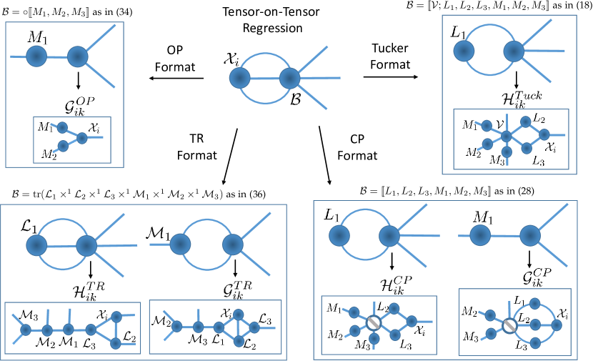
where HikCP=ik<2>CPsuperscriptsubscript𝐻𝑖𝑘𝐶𝑃superscriptsubscript𝑖𝑘expectation2𝐶𝑃H_{ik}^{CP}=\mathcal{H}_{ik<2>}^{CP} and ikCPsuperscriptsubscript𝑖𝑘𝐶𝑃\mathcal{H}_{ik}^{CP} is identical to the ikTKsuperscriptsubscript𝑖𝑘𝑇𝐾\mathcal{H}_{ik}^{TK} of (20), but for the fact that 𝒱𝒱\mathcal{V} is the diagonal tensor rp+lsuperscriptsubscript𝑟𝑝𝑙\mathcal{I}_{r}^{p+l}. (Fig. 5 displays ikCPsuperscriptsubscript𝑖𝑘𝐶𝑃\mathcal{H}_{ik}^{CP} for when p=l=3𝑝𝑙3p\!=\!l\!=\!3.) For k=1,,l𝑘1𝑙k=1,\!\hbox to10.00002pt{.\hss.\hss.},l, holding all parameters except Lksubscript𝐿𝑘L_{k} fixed makes (32) a MVMLR model with the MLE of Lksubscript𝐿𝑘L_{k} obtained as

vec(L^k)=(i=1nHikCPΣ1HikCP)1(i=1nHikCPΣ1vec(𝒴i)).vecsubscript^𝐿𝑘superscriptsuperscriptsubscript𝑖1𝑛superscriptsubscript𝐻𝑖𝑘𝐶𝑃superscriptΣ1superscriptsuperscriptsubscript𝐻𝑖𝑘𝐶𝑃1superscriptsubscript𝑖1𝑛superscriptsubscript𝐻𝑖𝑘𝐶𝑃superscriptΣ1vecsubscript𝒴𝑖\operatorname{vec}(\widehat{L}_{k})\!=\!\Big{(}\sum\limits_{i=1}^{n}H_{ik}^{CP}\Sigma^{-1}{H_{ik}^{CP}}^{\prime}\Big{)}^{-1}\Big{(}\sum\limits_{i=1}^{n}H_{ik}^{CP}\Sigma^{-1}\operatorname{vec}{(\mathcal{Y}_{i})}\Big{)}. (33)

The matrices i=1nHikCPΣ1vec(𝒴i)superscriptsubscript𝑖1𝑛superscriptsubscript𝐻𝑖𝑘𝐶𝑃superscriptΣ1vecsubscript𝒴𝑖\sum_{i=1}^{n}H_{ik}^{CP}\Sigma^{-1}\operatorname{vec}{(\mathcal{Y}_{i})}, i=1nHikCPΣ1HikCPsuperscriptsubscript𝑖1𝑛superscriptsubscript𝐻𝑖𝑘𝐶𝑃superscriptΣ1superscriptsuperscriptsubscript𝐻𝑖𝑘𝐶𝑃\sum_{i=1}^{n}H_{ik}^{CP}\Sigma^{-1}{H_{ik}^{CP}}^{\prime} are substantially simplified in Section S1-E1. As summarized in Fig. 5, the tensors ikCPsuperscriptsubscript𝑖𝑘𝐶𝑃\mathcal{H}_{ik}^{CP} and 𝒢ikCPsuperscriptsubscript𝒢𝑖𝑘𝐶𝑃\mathcal{G}_{ik}^{CP} play a critical role in the estimation of Mksubscript𝑀𝑘M_{k} and Lksubscript𝐿𝑘L_{k} through (29) and (32), permitting the use of standard MVMLR and MLR estimation methods. From (8), we deduce that the j𝑗jth columns of all the factor matrices in the CP decomposition (28) are identifiable only up to a constant. So we constrain the columns to have unit norm. The MLEs of our parameters are obtained using a block-relaxation algorithm, as outlined in Algorithm 2.

Initial Values : k=0,σ^2(0),L^2(0),L^3(0),,L^l(0),𝑘0superscript^𝜎20superscriptsubscript^𝐿20superscriptsubscript^𝐿30superscriptsubscript^𝐿𝑙0k=0,\widehat{\sigma}^{2(0)},\widehat{L}_{2}^{(0)},\widehat{L}_{3}^{(0)},\!\hbox to10.00002pt{.\hss.\hss.},\widehat{L}_{l}^{(0)}, M^1(0),M^2(0),,M^p(0)superscriptsubscript^𝑀10superscriptsubscript^𝑀20superscriptsubscript^𝑀𝑝0\widehat{M}_{1}^{(0)},\widehat{M}_{2}^{(0)},\!\hbox to10.00002pt{.\hss.\hss.},\widehat{M}_{p}^{(0)}
1 Center the data while saving the means 𝒳¯¯𝒳\mathcal{\bar{X}}, 𝒴¯¯𝒴\mathcal{\bar{Y}}.
2 while convergence criteria is not met do
3       for j=1,2,,l𝑗12𝑙j=1,2,\!\hbox to10.00002pt{.\hss.\hss.},l do
4            L^j(k+1)superscriptsubscript^𝐿𝑗𝑘1\widehat{L}_{j}^{(k+1)} as per (33) and normalize its columns
5       end for
6      for j=1,2,,p1𝑗12𝑝1j=1,2,\!\hbox to10.00002pt{.\hss.\hss.},p-1 do
7            (M^k(k+1),Σ^k(k+1))superscriptsubscript^𝑀𝑘𝑘1superscriptsubscript^Σ𝑘𝑘1(\widehat{M}_{k}^{(k+1)},\widehat{\Sigma}_{k}^{(k+1)}) as per (31) and normalize the columns of M^k(k+1)superscriptsubscript^𝑀𝑘𝑘1\widehat{M}_{k}^{(k+1)}
8       end for
9      (M^p(k+1),Σ^p(k+1))superscriptsubscript^𝑀𝑝𝑘1superscriptsubscript^Σ𝑝𝑘1(\widehat{M}_{p}^{(k+1)},\widehat{\Sigma}_{p}^{(k+1)}) as per (31)
10       σ^2(k+1)superscript^𝜎2𝑘1\widehat{\sigma}^{2(k+1)} as per (39)
11       Normalize the columns of M^p(k+1)superscriptsubscript^𝑀𝑝𝑘1\widehat{M}_{p}^{(k+1)} while setting 𝝀^(k+1)superscriptbold-^𝝀𝑘1\bm{\widehat{\lambda}}^{(k+1)} to those norms
12       k=k+1𝑘𝑘1k=k+1
13 end while
Υ^=𝒴¯𝒳¯|^CP^Υ¯𝒴inner-product¯𝒳subscript^𝐶𝑃\widehat{\Upsilon}=\mathcal{\bar{Y}}-\langle\mathcal{\bar{X}}|\mathcal{\widehat{B}}_{CP}\rangle
Algorithm 2 Block-relaxation algorithm for ToTR (13) with CP formatted \mathcal{B}
OP format

For an OP-formatted \mathcal{B}, i.e.,

OP=[[M1,,Mp]],\mathcal{B}_{OP}=\circ[\![M_{1},\!\hbox to10.00002pt{.\hss.\hss.},M_{p}]\!], (34)

we use Theorem II.1(b) to express (15) as

𝒴i=[[𝒳i;M1,,Mp]]+i.subscript𝒴𝑖delimited-[]subscript𝒳𝑖subscript𝑀1subscript𝑀𝑝subscript𝑖\mathcal{Y}_{i}=[\![\mathcal{X}_{i};M_{1},\!\hbox to10.00002pt{.\hss.\hss.},M_{p}]\!]+\mathcal{E}_{i}. (35)

We estimate the parameters in (35) by applying the k𝑘kth mode matricization for each k=1,,p𝑘1𝑝k=1,\!\hbox to10.00002pt{.\hss.\hss.},p on both sides as 𝒴i(k)=MkGikOP+Ei,subscriptsubscript𝒴𝑖𝑘subscript𝑀𝑘superscriptsubscript𝐺𝑖𝑘𝑂𝑃subscript𝐸𝑖{\mathcal{Y}_{i}}_{(k)}=M_{k}G_{ik}^{OP}+E_{i}, where GikOP=𝒳i(k)(j=p,jk1Mj)superscriptsubscript𝐺𝑖𝑘𝑂𝑃subscript𝒳𝑖𝑘superscriptsubscripttensor-productformulae-sequence𝑗𝑝𝑗𝑘1superscriptsubscript𝑀𝑗G_{ik}^{OP}=\mathcal{X}_{i(k)}\Big{(}\bigotimes_{j=p,j\neq k}^{1}M_{j}^{\prime}\Big{)} and Eiiid𝒩[mk,mk](0,σ2Σk,Σk)subscript𝐸𝑖𝑖𝑖𝑑similar-tosubscript𝒩superscriptsubscript𝑚𝑘subscript𝑚𝑘0superscript𝜎2subscriptΣ𝑘subscriptΣ𝑘E_{i}\overset{iid}{\sim}\operatorname{\mathcal{N}}_{[m_{k},m_{-k}]^{\prime}}(0,\sigma^{2}\Sigma_{k},\Sigma_{-k}). Given the similarities between this formulation and (29), the MLEs of the factor matrices are as in (33) but with GikOPsuperscriptsubscript𝐺𝑖𝑘𝑂𝑃G_{ik}^{OP} instead of GikCPsuperscriptsubscript𝐺𝑖𝑘𝐶𝑃G_{ik}^{CP}. The optimization procedure is similar to Algorithm 2, with the difference again that M1,,Mp1subscript𝑀1subscript𝑀𝑝1M_{1},\!\hbox to10.00002pt{.\hss.\hss.},M_{p-1} are normalized to have unit Frobenius norm. We conclude by noting that (35) is the multilinear tensor regression setup of [13], and for p=2𝑝2p=2 is the matrix-variate regression framework of [56] and [57]. So the OP format frames existing methodology within the ToTR framework.

TR format

Let \mathcal{B} have TR format (11), i.e.

TR=tr(1×12×1×1l×11×12×1×1p),subscript𝑇𝑅trsuperscript1superscript1superscript1superscript1superscript1superscript1superscript1subscript1subscript2subscript𝑙subscript1subscript2subscript𝑝\mathcal{B}_{TR}=\operatorname{tr}(\mathcal{L}_{1}\times^{1}\!\mathcal{L}_{2}\times^{1}\!\!\hbox to10.00002pt{.\hss.\hss.}\times^{1}\!\mathcal{L}_{l}\times^{1}\!\mathcal{M}_{1}\times^{1}\!\mathcal{M}_{2}\times^{1}\!\!\hbox to10.00002pt{.\hss.\hss.}\times^{1}\!\mathcal{M}_{p}), (36)

of TR rank (s1,,sl,g1,,gp)subscript𝑠1subscript𝑠𝑙subscript𝑔1subscript𝑔𝑝(s_{1},\!\hbox to10.00002pt{.\hss.\hss.},s_{l},g_{1},\!\hbox to10.00002pt{.\hss.\hss.},g_{p}), where jsubscript𝑗\mathcal{L}_{j} and ksubscript𝑘\mathcal{M}_{k} are third order tensor of sizes (sj1×hj×sj)subscript𝑠𝑗1subscript𝑗subscript𝑠𝑗(s_{j-1}\times h_{j}\times s_{j}) and (gk1×mk×gk)subscript𝑔𝑘1subscript𝑚𝑘subscript𝑔𝑘(g_{k-1}\times m_{k}\times g_{k}) respectively, for all j=1,,l𝑗1𝑙j=1,\!\hbox to10.00002pt{.\hss.\hss.},l and k=1,,p𝑘1𝑝k=1,\!\hbox to10.00002pt{.\hss.\hss.},p, and where g0=slsubscript𝑔0subscript𝑠𝑙g_{0}\!=\!s_{l} and s0=gpsubscript𝑠0subscript𝑔𝑝s_{0}\!=\!g_{p}. The TR format reduces the number of unconstrained parameters in \mathcal{B} from i=1lhii=1pmisuperscriptsubscriptproduct𝑖1𝑙subscript𝑖superscriptsubscriptproduct𝑖1𝑝subscript𝑚𝑖\prod_{i=1}^{l}h_{i}\prod_{i=1}^{p}m_{i} to j=1lsj1hjsj+k=1pgk1mkgksuperscriptsubscript𝑗1𝑙subscript𝑠𝑗1subscript𝑗subscript𝑠𝑗superscriptsubscript𝑘1𝑝subscript𝑔𝑘1subscript𝑚𝑘subscript𝑔𝑘\sum_{j=1}^{l}s_{j-1}h_{j}s_{j}+\sum_{k=1}^{p}g_{k-1}m_{k}g_{k}. To estimate parameters, we apply the k𝑘kth mode matricization for k=1,,p𝑘1𝑝k=1,\!\hbox to10.00002pt{.\hss.\hss.},p on both sides of (13), yielding

𝒴i(k)=k(2)GikTR+Ei,Eiiid𝒩[mk,mk](0,σ2Σk,Σk),subscriptsubscript𝒴𝑖𝑘subscript𝑘2superscriptsubscript𝐺𝑖𝑘𝑇𝑅subscript𝐸𝑖subscript𝐸𝑖𝑖𝑖𝑑similar-tosubscript𝒩superscriptsubscript𝑚𝑘subscript𝑚𝑘0superscript𝜎2subscriptΣ𝑘subscriptΣ𝑘{\mathcal{Y}_{i}}_{(k)}=\mathcal{M}_{k(2)}G_{ik}^{TR}+E_{i},\quad E_{i}\overset{iid}{\sim}\operatorname{\mathcal{N}}_{[m_{k},m_{-k}]^{\prime}}(0,\sigma^{2}\Sigma_{k},\Sigma_{-k}), (37)

and the vectorization for k=1,,l𝑘1𝑙k=1,\!\hbox to10.00002pt{.\hss.\hss.},l, which gives us

vec(𝒴i)=HikTRvec(k)+𝒆i,𝒆iiid𝒩m(0,σ2Σ),vecsubscript𝒴𝑖superscriptsubscript𝐻𝑖𝑘𝑇𝑅vecsubscript𝑘subscript𝒆𝑖subscript𝒆𝑖𝑖𝑖𝑑similar-tosubscript𝒩𝑚0superscript𝜎2Σ\operatorname{vec}(\mathcal{Y}_{i})=H_{ik}^{TR}\operatorname{vec}(\mathcal{L}_{k})+\bm{e}_{i},\quad\bm{e}_{i}\overset{iid}{\sim}\operatorname{\mathcal{N}}_{m}(0,\sigma^{2}\Sigma), (38)

where GikTRsuperscriptsubscript𝐺𝑖𝑘𝑇𝑅G_{ik}^{TR} and HikTRsuperscriptsubscript𝐻𝑖𝑘𝑇𝑅H_{ik}^{TR} are matrices as defined in Section S1-E2. Fig. 5 represents tensor-variate versions of HikTRsuperscriptsubscript𝐻𝑖𝑘𝑇𝑅H_{ik}^{TR} and GikTRsuperscriptsubscript𝐺𝑖𝑘𝑇𝑅G_{ik}^{TR} for when p=l=3𝑝𝑙3p\!=\!l\!=\!3. Because (29) and (32) are similar to (37) and (38), our ML estimators mirror the CP format case but by replacing (HikCP,GikCP)superscriptsubscript𝐻𝑖𝑘𝐶𝑃superscriptsubscript𝐺𝑖𝑘𝐶𝑃(H_{ik}^{CP},G_{ik}^{CP}) with (HikTR,GikTR)superscriptsubscript𝐻𝑖𝑘𝑇𝑅superscriptsubscript𝐺𝑖𝑘𝑇𝑅(H_{ik}^{TR},G_{ik}^{TR}). In this case, estimating (Mk,vec(Lk))subscript𝑀𝑘vecsubscript𝐿𝑘(M_{k},\operatorname{vec}(L_{k})) corresponds to estimating (k(2),vec(k))subscript𝑘2vecsubscript𝑘(\mathcal{M}_{k(2)},\operatorname{vec}(\mathcal{L}_{k})). The optimization procedure is similar to Algorithm 2, with the difference in this case being that each factor tensor, other than psubscript𝑝\mathcal{M}_{p}, is scaled to have unit Frobenius norm. We end here by noting that the special TR case of TT format has been used for ToTR in [32], with Σ=IΣ𝐼\Sigma=I, and hence Σk=IsubscriptΣ𝑘𝐼\Sigma_{k}=I for all k𝑘k.

Concluding Remarks

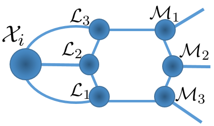
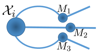
Fig. 5 summarizes our estimation methods for \mathcal{B} of different formats.

Refer to caption
Figure 5: Equivalent tensor-network diagrams for 𝒳i,subscript𝒳𝑖\langle\mathcal{X}_{i},\mathcal{B}\rangle when p=l=3𝑝𝑙3p=l=3, which can be expressed in multiple ways depending on the tensor factor to be estimated and the type of low-rank on \mathcal{B} (which are illustrated in Fig. 4). By choosing the tensors 𝒢iksubscript𝒢𝑖𝑘\mathcal{G}_{ik} and iksubscript𝑖𝑘\mathcal{H}_{ik}, the tensors M1subscript𝑀1M_{1} and 1subscript1\mathcal{M}_{1} can be estimated using multivariate multiple linear regression, and the tensors L1subscript𝐿1L_{1} and 1subscript1\mathcal{L}_{1} can be estimated using multiple linear regression, respectively. In these cases, matricized versions of 𝒢iksubscript𝒢𝑖𝑘\mathcal{G}_{ik} and iksubscript𝑖𝑘\mathcal{H}_{ik} are part of the design matrix.

We see that in many cases, an algorithmic block can be made to correspond to a linear model by appropriate choice of 𝒢iksubscript𝒢𝑖𝑘\mathcal{G}_{ik} or iksubscript𝑖𝑘\mathcal{H}_{ik}. Then, fitting a tensor-response linear model involves sequentially fitting smaller-dimensional linear models (one for each tensor factor) until convergence. This intuition behind the estimation of \mathcal{B} is not restricted to the TK, CP, OP and TR formats, but can also help guide estimation algorithms for other formats such as the hierarchical Tucker and the tensor tree formats [58, 59].

While the OP format has the advantage of parsimony, it does not allow for the level of recovery to be adjusted through a tensor rank (as will be illustrated in Section III and Fig. 6). The CP format is a more attractive alternative, since it is the natural generalization of the low-rank matrix format (a tensor with CP rank k𝑘k is the sum of k𝑘k tensors with CP rank 111). However, the CP format can be too restrictive in some scenarios, such as when the tensor modes have very different sizes. In such cases, the Tucker format provides a more appealing alternative. Moreover, a Tucker-formatted tensor has the interpretation of being a core tensor that is stretched on each mode by a tall matrix. However, its disadvantage is that the core tensor has the same number of modes as the original tensor, making it impractical in very high-order tensor scenarios. In such situations, the TR format is preferred because each additional tensor-mode requires only one additional tensor factor.

II-C3 Estimation of σ2superscript𝜎2\sigma^{2}

In all cases, the estimation of ΣksubscriptΣ𝑘\Sigma_{k} involves finding the sum of squared errors along the k𝑘k-mode Sksubscript𝑆𝑘S_{k}, as in equations (26) and (30). Given the estimated Σ^ksubscript^Σ𝑘\widehat{\Sigma}_{k} and Sksubscript𝑆𝑘S_{k}, the estimate of σ2superscript𝜎2\sigma^{2} is very cheap and given as

σ^2=1nmtr(Σ^kSk).superscript^𝜎21𝑛𝑚trsubscript^Σ𝑘subscript𝑆𝑘\widehat{\sigma}^{2}=\dfrac{1}{nm}\operatorname{tr}(\widehat{\Sigma}_{k}S_{k}). (39)

Thus σ^2superscript^𝜎2\widehat{\sigma}^{2} is obtained alternatively within each iteration. Moreover, the log-likelihood function evaluated at the current estimated values is greatly simplified based on σ^2superscript^𝜎2\widehat{\sigma}^{2} as

=nm2[1+log(2πσ^2)+k=1plog|Σ^k|/mk].𝑛𝑚2delimited-[]12𝜋superscript^𝜎2superscriptsubscript𝑘1𝑝subscript^Σ𝑘subscript𝑚𝑘\ell=-\dfrac{nm}{2}\left[1+\log(2\pi\widehat{\sigma}^{2})+\sum_{k=1}^{p}\log|\widehat{\Sigma}_{k}|/m_{k}\right].

II-C4 Initialization and convergence

For local optimality, we need the two conditions that the log-likelihood \ell is jointly continuous and that the set {𝜽:(𝜽)(𝜽(0))}conditional-set𝜽𝜽superscript𝜽0\{\bm{\theta}:\ell(\bm{\theta})\geq\ell(\bm{\theta}^{(0)})\}, for a set of initial values 𝜽(0)superscript𝜽0\bm{\theta}^{(0)}, is compact [53]. These conditions are satisfied because of the TVN distributional assumption on our errors, as long as the initial values satisfy the constraints on the parameters. We initialized Σk=ImksubscriptΣ𝑘subscript𝐼subscript𝑚𝑘\Sigma_{k}=I_{m_{k}} and the tensor factor entries in \mathcal{B} with draws from the 𝒰(0,1)𝒰01\mathcal{U}(0,1) distribution. With the TK format, Mksubscript𝑀𝑘M_{k} has the constraint MkΣk1Mk=Idksuperscriptsubscript𝑀𝑘superscriptsubscriptΣ𝑘1subscript𝑀𝑘subscript𝐼subscript𝑑𝑘M_{k}^{\prime}\Sigma_{k}^{-1}M_{k}=I_{d_{k}} for k=1,,p𝑘1𝑝k=1,\!\hbox to10.00002pt{.\hss.\hss.},p, so we used Σk12UsuperscriptsubscriptΣ𝑘12𝑈\Sigma_{k}^{\frac{1}{2}}U as its initializer, with U𝑈U having the left singular vectors of a random matrix of the same order as Mksubscript𝑀𝑘M_{k}. We also suggest using identity matrices to initialize Σ1,,ΣpsubscriptΣ1subscriptΣ𝑝\Sigma_{1},\dots,\Sigma_{p} and σ2superscript𝜎2\sigma^{2} can be initialized with 1. Our algorithms are declared to converge when we have negligible changes in the loglikelihood, as simplified in Section II-C3. A different criteria is the difference in norm +σ2Σnormnormsuperscript𝜎2Σ||\mathcal{B}||+||\sigma^{2}\Sigma||, where σ2Σ=σk=1pΣknormsuperscript𝜎2Σ𝜎superscriptsubscriptproduct𝑘1𝑝normsubscriptΣ𝑘||\sigma^{2}\Sigma||=\sigma\prod_{k=1}^{p}||\Sigma_{k}|| and norm||\mathcal{B}|| simplifies as per format:

  • for TKsubscript𝑇𝐾\mathcal{B}_{TK}, with Aqsuperscript𝐴𝑞A^{q} as the Q matrix from the LQ decomposition of A𝐴A [44], we have TK=[[𝒱;L1q,,Llq,M1q,,Mpq]]normsubscript𝑇𝐾normdelimited-[]𝒱superscriptsubscript𝐿1𝑞superscriptsubscript𝐿𝑙𝑞superscriptsubscript𝑀1𝑞superscriptsubscript𝑀𝑝𝑞||\mathcal{B}_{TK}||=||[\![\mathcal{V};L_{1}^{q},\!\hbox to10.00002pt{.\hss.\hss.},L_{l}^{q},M_{1}^{q},\!\hbox to10.00002pt{.\hss.\hss.},M_{p}^{q}]\!]||.

  • for CPsubscript𝐶𝑃\mathcal{B}_{CP}, ||CP||2=k,l=1R{diag(𝝀)[i=1l(LiLi)][i=1p(MiMi)]}(k,l)||\mathcal{B}_{CP}||^{2}=\sum_{k,l=1}^{R}\big{\{}diag(\bm{\lambda})[*_{i=1}^{l}(L_{i}^{\prime}L_{i})]*[*_{i=1}^{p}(M_{i}^{\prime}M_{i})]\big{\}}(k,l), where “*” is the Hadamard, or entry-wise product [44].

  • for OPsubscript𝑂𝑃\mathcal{B}_{OP}, OP=i=1pMinormsubscript𝑂𝑃superscriptsubscriptproduct𝑖1𝑝normsubscript𝑀𝑖||\mathcal{B}_{OP}||=\prod_{i=1}^{p}||M_{i}||.

II-D Properties of our estimators

II-D1 Computational complexity

We derive the computational complexity of our estimation algorithms. Recall that in all cases the response 𝒴i×k=1pmksubscript𝒴𝑖superscriptsuperscriptsubscript𝑘1𝑝absentsubscript𝑚𝑘\mathcal{Y}_{i}\in\mathbb{R}^{\times_{k=1}^{p}m_{k}} and the covariate 𝒳i×k=1lhksubscript𝒳𝑖superscriptsuperscriptsubscript𝑘1𝑙absentsubscript𝑘\mathcal{X}_{i}\in\mathbb{R}^{\times_{k=1}^{l}h_{k}} where l𝑙l and p𝑝p are considered fixed. WLOG, we assume that m1=max{m1,,mp}subscript𝑚1subscript𝑚1subscript𝑚𝑝m_{1}\!=\!\max\{m_{1},\dots,m_{p}\} and h1=max{h1,,hl}subscript1subscript1subscript𝑙h_{1}\!=\!\max\{h_{1},\dots,h_{l}\}.

Theorem II.3.

The computational complexity of our ToTR algorithms when \mathcal{B} has

  1. 1.

    the TK format of Section II-C2, with d=q=1pdq𝑑superscriptsubscriptproduct𝑞1𝑝subscript𝑑𝑞d=\prod_{q=1}^{p}d_{q}, d1=d/d1subscript𝑑1𝑑subscript𝑑1d_{-1}=d/d_{1}, c=q=1lcq𝑐superscriptsubscriptproduct𝑞1𝑙subscript𝑐𝑞c=\prod_{q=1}^{l}c_{q}, d1=max{d1,,dp}subscript𝑑1subscript𝑑1subscript𝑑𝑝d_{1}=\max\{d_{1},\dots,d_{p}\} and c1=max{c1,,cl}subscript𝑐1subscript𝑐1subscript𝑐𝑙c_{1}=\max\{c_{1},\dots,c_{l}\} and implemented in Algorithm 1 is 𝒪(nhc1+n2c+n2m1d1+nm12d1)+𝒪(nmd1)+𝒪(ncdh1+nc12h12d+h13c13)+𝒪(m13+nmm1)𝒪𝑛subscript𝑐1superscript𝑛2𝑐superscript𝑛2subscript𝑚1subscript𝑑1𝑛superscriptsubscript𝑚12subscript𝑑1𝒪𝑛𝑚subscript𝑑1𝒪𝑛𝑐𝑑subscript1𝑛superscriptsubscript𝑐12superscriptsubscript12𝑑superscriptsubscript13superscriptsubscript𝑐13𝒪superscriptsubscript𝑚13𝑛𝑚subscript𝑚1\mathcal{O}\big{(}nhc_{1}+n^{2}c+n^{2}m_{1}d_{-1}+nm_{1}^{2}d_{-1}\big{)}+\mathcal{O}\big{(}nmd_{1}\big{)}+\mathcal{O}\big{(}ncdh_{1}+nc_{1}^{2}h_{1}^{2}d+h_{1}^{3}c_{1}^{3}\big{)}+\mathcal{O}\big{(}m_{1}^{3}+nmm_{1}\big{)}.

  2. 2.

    the CP format of Section II-C2 and implemented in Algorithm 2 is 𝒪(nh12r2+nrm+rm12+m13+h13r3+nrh+m1r2+nmm1).𝒪𝑛superscriptsubscript12superscript𝑟2𝑛𝑟𝑚𝑟superscriptsubscript𝑚12superscriptsubscript𝑚13superscriptsubscript13superscript𝑟3𝑛𝑟subscript𝑚1superscript𝑟2𝑛𝑚subscript𝑚1\mathcal{O}\big{(}nh_{1}^{2}r^{2}+nrm+rm_{1}^{2}+m_{1}^{3}+h_{1}^{3}r^{3}+nrh+m_{1}r^{2}+nmm_{1}\big{)}.

  3. 3.

    the TR format, as described in Section II-C2 and with g0g1=max{gk1gk:k=1,2,p}subscript𝑔0subscript𝑔1:subscript𝑔𝑘1subscript𝑔𝑘𝑘12𝑝g_{0}g_{1}=\max\{g_{k-1}g_{k}:k=1,2,\dots p\}, s0s1=max{sk1sk:k=1,2,l}subscript𝑠0subscript𝑠1:subscript𝑠𝑘1subscript𝑠𝑘𝑘12𝑙s_{0}s_{1}=\max\{s_{k-1}s_{k}:k=1,2,\dots l\}, g=max{g0,g1}𝑔subscript𝑔0subscript𝑔1g=\max\{g_{0},g_{1}\}, g0g1m1subscript𝑔0subscript𝑔1subscript𝑚1g_{0}g_{1}\leq m_{1} is 𝒪(mg1g0gp+hnssl+mh12s02s12+h13s03s13)+𝒪(hs1s0sl+m13+g03g13+nmm1).𝒪𝑚subscript𝑔1subscript𝑔0subscript𝑔𝑝𝑛𝑠subscript𝑠𝑙𝑚superscriptsubscript12superscriptsubscript𝑠02superscriptsubscript𝑠12superscriptsubscript13superscriptsubscript𝑠03superscriptsubscript𝑠13𝒪subscript𝑠1subscript𝑠0subscript𝑠𝑙superscriptsubscript𝑚13superscriptsubscript𝑔03superscriptsubscript𝑔13𝑛𝑚subscript𝑚1\mathcal{O}\big{(}mg_{1}g_{0}g_{p}+hnss_{l}+mh_{1}^{2}s_{0}^{2}s_{1}^{2}+h_{1}^{3}s_{0}^{3}s_{1}^{3}\big{)}+\mathcal{O}\big{(}hs_{1}s_{0}s_{l}+m_{1}^{3}+g_{0}^{3}g_{1}^{3}+nmm_{1}\big{)}.

Proof.

See Sections S1-G1 - S1-G4 for the proofs. ∎

In all cases we have the term 𝒪(nmm1)𝒪𝑛𝑚subscript𝑚1\mathcal{O}(nmm_{1}), which is the complexity of obtaining the sum of square errors Sksubscript𝑆𝑘S_{k} of equation (26) across the largest tensor-response mode, and it is necessary for obtaining the scale matrices Σ1,,ΣpsubscriptΣ1subscriptΣ𝑝\Sigma_{1},\!\hbox to10.00002pt{.\hss.\hss.},\Sigma_{p}. In many cases this term will dominate the computational complexity. However, O(nmm1)𝑂𝑛𝑚subscript𝑚1O(nmm_{1}) is considerably smaller than O(nm2)𝑂𝑛superscript𝑚2O(nm^{2}), which would be the case where our complexity increases quadratically with the dimensionality of the tensor response. We also note that in all cases, the cubic terms are WRT the tensor ranks, which can be considered negligible because such ranks are often chosen to be small, in the spirit of scientific parsimony. Finally, for the TK format, some of the factors can assumed to be identity matrices, allowing us to further reduce the complexity. (See Section S1-G3 for the computational complexity of the OP format under specific conditions.)

II-D2 Asymptotic sampling distributions

We now derive the asymptotic distributions of our model-estimated parameters, specifically, the linear component and the covariance component (Section S1-M).

We first explore the limiting distribution of the estimated linear components vec(^)vec^\operatorname{vec}(\mathcal{\widehat{B}}), which in all cases is multivariate normal with mean vec()vec\operatorname{vec}(\mathcal{B}) satisfying the same low-rank format of vec(^)vec^\operatorname{vec}(\mathcal{\widehat{B}}). For the Tucker format, we first show that the vectorized core tensor vec(𝒱^)vec^𝒱\operatorname{vec}(\mathcal{\widehat{V}}) follows a non-singular multivariate normal distribution, and therefore by Slutsky’s theorem vec(^)vec^\operatorname{vec}(\mathcal{\widehat{B}}) follows a singular multivariate normal distribution, where the singularity of the covariance matrix constraints the limiting distribution to the original low-rank Tucker format. For the CP, TR and OP cases we first show that the low-rank format factors in \mathcal{B} are jointly normally distributed. Therefore, by the Delta method the estimated tensors ^^\mathcal{\widehat{B}} in vectorized form are asymptotic normally distributed. In this case the resulting multivariate normal distribution is also singular, but these are only approximations to the CP, TR or OP formats and not constraints on the limiting distributions like it is the case for the Tucker format.

For the remainder of this paper, we define hi=1lhiapproaches-limitsuperscriptsubscriptproduct𝑖1𝑙subscript𝑖h\doteq\prod_{i=1}^{l}h_{i}, Mi=p1Miapproaches-limit𝑀superscriptsubscripttensor-product𝑖𝑝1subscript𝑀𝑖M\doteq\bigotimes_{i=p}^{1}M_{i} and Li=l1Liapproaches-limit𝐿superscriptsubscripttensor-product𝑖𝑙1subscript𝐿𝑖L\doteq\bigotimes_{i=l}^{1}L_{i}. We first assume that (15) holds without an intercept.

Theorem II.4.

Let (15) hold with TKsubscript𝑇𝐾\mathcal{B}\equiv\mathcal{B}_{TK} of Tucker format as in (18) and let X=[vec(𝒳1)vec(𝒳n)]𝑋delimited-[]𝑣𝑒𝑐subscript𝒳1𝑣𝑒𝑐subscript𝒳𝑛X=[vec(\mathcal{X}_{1})\!\hbox to10.00002pt{.\hss.\hss.}vec(\mathcal{X}_{n})] and ^TK=[[𝒱^;L^1,L^2,,L^l,M^1,M^2,,M^p]]subscript^𝑇𝐾delimited-[]^𝒱subscript^𝐿1subscript^𝐿2subscript^𝐿𝑙subscript^𝑀1subscript^𝑀2subscript^𝑀𝑝\mathcal{\widehat{B}}_{TK}=[\![\mathcal{\widehat{V}};\widehat{L}_{1},\widehat{L}_{2},\!\hbox to10.00002pt{.\hss.\hss.},\widehat{L}_{l},\widehat{M}_{1},\widehat{M}_{2},\!\hbox to10.00002pt{.\hss.\hss.},\widehat{M}_{p}]\!]. Then as n𝑛n\rightarrow\infty

vec(^TK)𝑑𝒩mh(vec(TK),σ2(MM)(PL(XX)1PL)),vecsubscript^𝑇𝐾𝑑subscript𝒩𝑚vecsubscript𝑇𝐾tensor-productsuperscript𝜎2𝑀superscript𝑀subscript𝑃𝐿superscript𝑋superscript𝑋1subscript𝑃𝐿\operatorname{vec}(\mathcal{\widehat{B}}_{TK})\!\overset{d}{\rightarrow}\!\operatorname{\mathcal{N}}_{mh}\!\!\big{(}\operatorname{vec}(\mathcal{B}_{TK}),\sigma^{2}(MM^{\prime})\otimes(P_{L}(XX^{\prime})^{-1}P_{L})\big{)},

where PL=i=l1Pisubscript𝑃𝐿superscriptsubscripttensor-product𝑖𝑙1subscript𝑃𝑖P_{L}=\bigotimes_{i=l}^{1}P_{i} and Pi=Li(LiLi)1Li.subscript𝑃𝑖subscript𝐿𝑖superscriptsuperscriptsubscript𝐿𝑖subscript𝐿𝑖1superscriptsubscript𝐿𝑖P_{i}=L_{i}(L_{i}^{\prime}L_{i})^{-1}L_{i}^{\prime}.

Proof.

See Section S1-H. ∎

The limiting distribution in Theorem II.4 is TVN when XX𝑋superscript𝑋XX^{\prime} has a Kronecker structure: examples include factorial designs and B-splines [60]. Here we present one such case.

Corollary II.1.

When ^TKsubscript^𝑇𝐾\mathcal{\widehat{B}}_{TK} is used to estimate a balanced TANOVA with q𝑞q units for each factor combination, then for 𝐬=[h1,h2,,hl,m1,m2,,mp]𝐬superscriptsubscript1subscript2subscript𝑙subscript𝑚1subscript𝑚2subscript𝑚𝑝\bm{s}=[h_{1},h_{2},\!\hbox to10.00002pt{.\hss.\hss.},h_{l},m_{1},m_{2},\!\hbox to10.00002pt{.\hss.\hss.},m_{p}]^{\prime}, as n𝑛n\rightarrow\infty

^TK𝑑𝒩𝒔(,σ2qP1,P2,,Pl,M1M1,M2M2,MpMp).subscript^𝑇𝐾𝑑subscript𝒩𝒔superscript𝜎2𝑞subscript𝑃1subscript𝑃2subscript𝑃𝑙subscript𝑀1superscriptsubscript𝑀1subscript𝑀2superscriptsubscript𝑀2subscript𝑀𝑝superscriptsubscript𝑀𝑝\mathcal{\widehat{B}}_{TK}\overset{d}{\rightarrow}\operatorname{\mathcal{N}}_{\bm{s}}\big{(}\mathcal{B},\dfrac{\sigma^{2}}{q}P_{1},P_{2},\!\hbox to10.00002pt{.\hss.\hss.},P_{l},M_{1}M_{1}^{\prime},M_{2}M_{2}^{\prime}\!\hbox to10.00002pt{.\hss.\hss.},M_{p}M_{p}^{\prime}\big{)}.
Proof.

Here XX=qIh𝑋superscript𝑋𝑞subscript𝐼XX^{\prime}=qI_{h} and so the variance-covariance matrix in the limiting distribution of Theorem II.4 is (σ2/q)(MM)(i=l1Pi)tensor-productsuperscript𝜎2𝑞𝑀superscript𝑀superscriptsubscripttensor-product𝑖𝑙1subscript𝑃𝑖(\sigma^{2}/q)(MM^{\prime})\otimes(\bigotimes_{i=l}^{1}P_{i}), which is Kronecker-separable. The result follows from Definition II.2. ∎

The CP format case is similar to Theorem II.4.

Theorem II.5.

Consider (15) with CPsubscript𝐶𝑃\mathcal{B}\equiv\mathcal{B}_{CP} as in (28) and the ML estimator ^CP=[[L^1,L^2,,L^l,M^1,M^2,,M^p]].subscript^𝐶𝑃delimited-[]subscript^𝐿1subscript^𝐿2subscript^𝐿𝑙subscript^𝑀1subscript^𝑀2subscript^𝑀𝑝\mathcal{\widehat{B}}_{CP}=[\![\widehat{L}_{1},\widehat{L}_{2},\!\hbox to10.00002pt{.\hss.\hss.},\widehat{L}_{l},\widehat{M}_{1},\widehat{M}_{2},\!\hbox to10.00002pt{.\hss.\hss.},\widehat{M}_{p}]\!]. Then

vec(^CP)𝑑𝒩mh(vec(CP),JCPRCP(InΣ)RCPJCP)vecsubscript^𝐶𝑃𝑑subscript𝒩𝑚vecsubscript𝐶𝑃subscript𝐽𝐶𝑃subscript𝑅𝐶𝑃tensor-productsubscriptI𝑛Σsuperscriptsubscript𝑅𝐶𝑃superscriptsubscript𝐽𝐶𝑃\operatorname{vec}(\mathcal{\widehat{B}}_{CP})\overset{d}{\rightarrow}\operatorname{\mathcal{N}}_{mh}\Big{(}\operatorname{vec}(\mathcal{B}_{CP}),J_{CP}R_{CP}(\operatorname{I}_{n}\otimes\Sigma)R_{CP}^{\prime}J_{CP}^{\prime}\Big{)}

as n𝑛n\rightarrow\infty. Here JCPsubscript𝐽𝐶𝑃J_{CP} is a Jacobian matrix and is given along with the block matrix RCPsubscript𝑅𝐶𝑃R_{CP} in Section S1-I.

Proof.

See Section S1-I. ∎

The sampling distributions of \mathcal{B} under the OP or TR formats are similar to the CP case, and are in theorem S1.2 of Section S1-J.

Theorem II.6.

For a model with intercept, as in (13), Theorems II.4 and II.5 also hold after centering the covariates.

Proof.

See Section S1-L. ∎

Section S1-M also discusses inference on the scale components Σ^1,Σ^2,,Σ^psubscript^Σ1subscript^Σ2subscript^Σ𝑝\widehat{\Sigma}_{1},\widehat{\Sigma}_{2},\!\hbox to10.00002pt{.\hss.\hss.},\widehat{\Sigma}_{p}. Theorem S1.3 establishes the asymptotic independence of the scale and the linear components, we find the Fisher information matrix WRT the scale parameters, and establish its singularity. Our results on the asymptotic distribution of the scale components are not unique to our regression methodology but also generally hold for the TVN distribution.

II-E Model selection or rank determination

For the CP, TR and TK formats, we determine optimal ranks using the Bayesian information criterion (BIC) [61, 62]. This calculation requires the loglikelihood that we simplified in Section II-C3. Section S1-F provides more details on rank determination (equivalently, model selection) and on the total number of calculations needed to obtain the BIC.

III Experimental Evaluations

We study estimation performance of the scale parameters and the low-rank linear component \mathcal{B} using simulation experiments on different ToTR models. Section III-A assesses the consistency of our estimators, and Section III-B evaluates the amounts of recovery that different low-rank formats have of \mathcal{B}, and the impact of noise on discrimination in a TANOVA framework.

III-A A TANOVA(2,2) model with low-rank formats
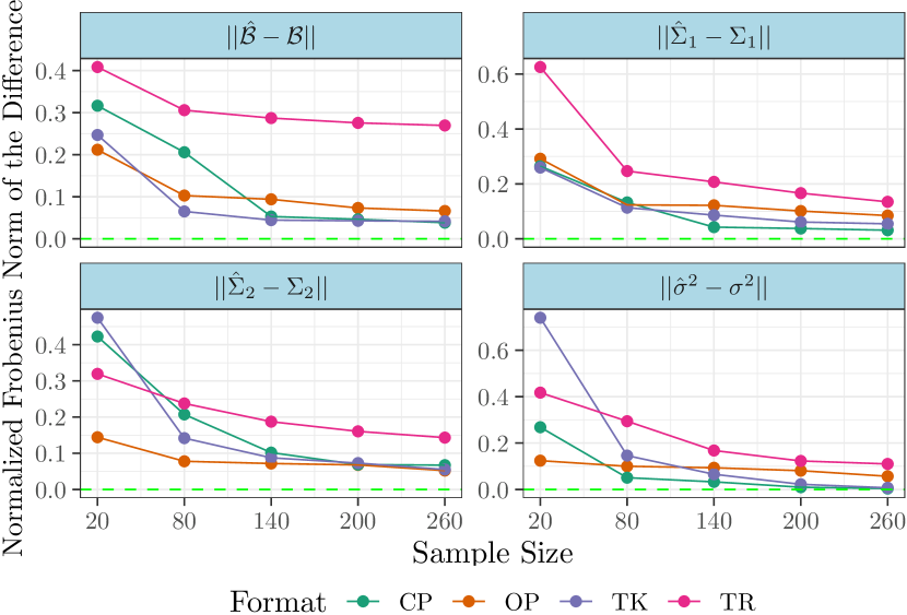
Refer to caption
Figure 6: Performance of the four models presented in Section III-A, each corresponding to a different format on \mathcal{B}. Each plot corresponds to the Frobenius norm of the difference between an estimated and true population parameter, against the sample size. We observe that in all cases, an increase in sample size leads to more accurate estimates.
Refer to caption
(a)
Refer to caption
(b)
Figure 7: (a) Results of fitting seven TANOVA(2,2) models on data simulated from (41). One model was fit assuming the OP format, and two models were fit for each of the TK, CP and TR formats: one with set ranks and another one with optimal ranks, as chosen by BIC. The two factors are the type of andean camelid (Guanaco, Llama, Vicuña, Alpaca) and the type of additive color RGB (red, green, blue). The Guanaco, Llama and Alpaca images are from Wikipedia Commons and the Vicuña image is from Encyclopædia Britannica. It is evident that while one cannot adjust the OP rank, increased rank for the TR, TK and CP formats result in more image restoration. (b) Monte-Carlo 95th quantiles of the Wilks’ ΛΛ\Lambda statistics that test the set of hypothesis in equation (42), for the OP, CP, TR and TK formats, five values of scalar variance σ2superscript𝜎2\sigma^{2} in the x-axis, and for both true and false null hypotheses. Large variabilities lead to larger test statistics when H0subscript𝐻0H_{0} is false, leading to weaker evidence against the null hypothesis. In all cases, CP, TR and TK formatting leads to more significant statistics when compared to the OP, even when the ranks are not optimal.

We simulated observations from the matrix-on-matrix regression (MoMR) model

Yijk=Xij|+Eijk,Eijkiid𝒩[6,7](0,σ2Σ1,Σ2)subscript𝑌𝑖𝑗𝑘inner-productsubscript𝑋𝑖𝑗subscript𝐸𝑖𝑗𝑘subscript𝐸𝑖𝑗𝑘𝑖𝑖𝑑similar-tosubscript𝒩superscript670superscript𝜎2subscriptΣ1subscriptΣ2Y_{ijk}=\langle X_{ij}|\mathcal{B}\rangle+E_{ijk},\quad E_{ijk}\overset{iid}{\sim}\operatorname{\mathcal{N}}_{[6,7]^{\prime}}(0,\sigma^{2}\Sigma_{1},\Sigma_{2}) (40)

where i=1,2,3,4𝑖1234i=1,2,3,4, j=1,2,3,4,5𝑗12345j=1,2,3,4,5 and Xijsubscript𝑋𝑖𝑗X_{ij} is a 4×5454\!\times\!5 matrix with 1 at the (i,j)𝑖𝑗(i,j)th position and zeroes everywhere else. We set σ2=1superscript𝜎21\sigma^{2}=1 and obtained Σ1subscriptΣ1\Sigma_{1} and Σ2subscriptΣ2\Sigma_{2} independently from Wishart distributions, that is, we obtained Σ1𝒲6(6,I6)similar-tosubscriptΣ1subscript𝒲66subscript𝐼6\Sigma_{1}\sim\mathcal{W}_{6}(6,I_{6}) and Σ2𝒲7(7,I7)similar-tosubscriptΣ2subscript𝒲77subscript𝐼7\Sigma_{2}\sim\mathcal{W}_{7}(7,I_{7}) before scaling each by their (1,1)11(1,1)th element. We obtained realizations from four MoMR models, one each for \mathcal{B} of TK, CP, TR and OP formats, and fit appropriate models to the data using the ML estimation procedures described in Section II-C. To study consistency properties of our estimators, we used k=1,4,7,10𝑘14710k=1,4,7,10 and 131313, meaning that our sample sizes ranged over n{20,80,140,200,260}𝑛2080140200260n\in\{20,80,140,200,260\}. An unstructured \mathcal{B} in this experiment would have 4×5×6×7=84045678404\times 5\times 6\times 7=840 entries, but \mathcal{B} has only 59 unconstrained parameters with the OP format and 45 unconstrained parameters when it is of CP format of rank 2. This number is only 60 when \mathcal{B} has TK format with rank (2,2,2,2) and 70 when it is of the TR format with rank (2,2,2,2). Thus, our lower-rank simulation framework had at least 91%percent9191\% fewer unconstrained parameters in \mathcal{B}. We simulated data from (40) using \mathcal{B}, σ2superscript𝜎2\sigma^{2}, Σ1subscriptΣ1\Sigma_{1} and Σ2subscriptΣ2\Sigma_{2} and estimated the parameters for each replication. Fig. 6 displays the Frobenius norm of the difference between the true and estimated parameters, and shows that as sample size increases, (^,σ^2,Σ^1,Σ^2)^superscript^𝜎2subscript^Σ1subscript^Σ2(\mathcal{\widehat{B}},\widehat{\sigma}^{2},\widehat{\Sigma}_{1},\widehat{\Sigma}_{2}) approach the true parameters (,σ2,Σ1,Σ2)superscript𝜎2subscriptΣ1subscriptΣ2(\mathcal{B},\sigma^{2},\Sigma_{1},\Sigma_{2}), demonstrating consistency of the estimators.

III-B Evaluating recovery and discrimination

We simulated 600 observations from the MoMR model

Yijk=Xij|+Eijk,Eijkiid𝒩[87,106](0,σ2Σ1,Σ2),subscript𝑌𝑖𝑗𝑘inner-productsubscript𝑋𝑖𝑗subscript𝐸𝑖𝑗𝑘subscript𝐸𝑖𝑗𝑘𝑖𝑖𝑑similar-tosubscript𝒩superscript871060superscript𝜎2subscriptΣ1subscriptΣ2Y_{ijk}=\langle X_{ij}|\mathcal{B}\rangle+E_{ijk},\quad E_{ijk}\overset{iid}{\sim}\operatorname{\mathcal{N}}_{[87,106]^{\prime}}(0,\sigma^{2}\Sigma_{1},\Sigma_{2}), (41)

where i=1,2,3,4𝑖1234i=1,2,3,4, j=1,2,3𝑗123j=1,2,3, Xijsubscript𝑋𝑖𝑗X_{ij} is a 4×3434\!\times\!3 matrix with 1 at the (i,j)𝑖𝑗(i,j)th position and zero elsewhere, and Υij=Xij|subscriptΥ𝑖𝑗inner-productsubscript𝑋𝑖𝑗\Upsilon_{ij}=\langle X_{ij}|\mathcal{B}\rangle corresponds to the pixel-wise logit transformation of the j𝑗jth additive color (Red, Green, Blue) of the i𝑖ith Andean camelid (Guanaco, Llama, Vicuña, Alpaca) images of Fig. 7(a). We set Σ1subscriptΣ1\Sigma_{1} and Σ2subscriptΣ2\Sigma_{2} to be AR(1) correlation matrices with coefficients 0.10.10.1 and 0.10.1-0.1 respectively, and σ2=1superscript𝜎21\sigma^{2}=1. Sans constaints, we have 3×4×87×106=11066434871061106643\times 4\times 87\times 106=110664 parameters in \mathcal{B}.

We fit (41) separately for TR-, TK-, CP- and OP-formatted \mathcal{B}, with ranks set to have similar number of unconstrained parameters in \mathcal{B}. The TR format with rank (3,3,5,3) had 2958 such parameters, the TK format with rank (4,4,9,9) had 3061 parameters, the CP format with rank 15 had 3001 parameters in \mathcal{B}, while the relatively inflexible OP format had 666 parameters. In all cases, the dimension of \mathcal{B} was reduced by over 97%. The estimated tensor \mathcal{B} in each case corresponds to the estimated color images of the four Andean camelids. Fig. 7(a) shows varying success of these four formats in recovering the underlying camelid image (true \mathcal{B}). The OP-estimated images are the least-resolved, with the reduced number of parameters for \mathcal{B} inadequate for recovery. But the other formats can adjust for the quantum of reduction in parameters through their ranks. We illustrate this aspect by fitting (41) with \mathcal{B} having the TK, CP and TR formats with optimal rank chosen by BIC, following Section II-E. Fig. 7(a) shows very good recovery of \mathcal{B} by these BIC-optimized ^^\mathcal{\widehat{B}}s, with unappreciable visual differences in all cases. In contrast, the model fit with unstructured \mathcal{B} and diagonal ΣΣ\Sigma, has a BIC of 1.64×1071.64superscript1071.64\times 10^{7}, while fitting a model with a similar \mathcal{B} but Kronecker-separable ΣΣ\Sigma has a BIC of 1.63×1071.63superscript1071.63\times 10^{7}. The CP, TK and TR formats therefore outperform these two alternatives when the ranks are tuned.

The TANOVA(2,2) formulation of (41) enables us to test

H0:𝒫1=𝒫2=𝒫3=𝒫4 vs. Ha:𝒫i𝒫i, for some ii{1,2,3,4}\displaystyle\begin{split}&\text{H}_{0}:\mathcal{P}_{1}=\mathcal{P}_{2}=\mathcal{P}_{3}=\mathcal{P}_{4}\hskip 40.00006pt\mbox{ vs. }\\ &\text{H}_{\text{a}}:\mathcal{P}_{i}\neq\mathcal{P}_{i^{*}},\mbox{ for some }i\neq i^{*}\in\{1,2,3,4\}\end{split} (42)

where 𝒫isubscript𝒫𝑖\mathcal{P}_{i} is a third-order tensor of size 3×87×1063871063\times 87\times 106 that contains the RGB slices of the i𝑖ith Andean camelid image. The usual Wilks’ ΛΛ\Lambda statistic [63] is Λ=|Σ^R|/|Σ^T|,Λsubscript^Σ𝑅subscript^Σ𝑇\Lambda=|\widehat{\Sigma}_{R}|/|\widehat{\Sigma}_{T}|, where Σ^Rsubscript^Σ𝑅\widehat{\Sigma}_{R} is the sample covariance matrix of the residuals and Σ^Tsubscript^Σ𝑇\widehat{\Sigma}_{T} is the sample covariance matrix of the simpler model’s residuals, which finds a common mean across all camelids. (Section S2 details the calculation of Σ^Rsubscript^Σ𝑅\widehat{\Sigma}_{R} and Σ^Tsubscript^Σ𝑇\widehat{\Sigma}_{T}.) We illustrate the role of σ2superscript𝜎2\sigma^{2} and the low-rank OP, TR, CP or TK formats in distinguishing the four camelids, as measured by the Wilks’ ΛΛ\Lambda test statistic, in Fig. 7(b), for σ=2,4,6,8,10𝜎246810\sigma=2,4,6,8,10. The value of ΛΛ\Lambda increases with σ2superscript𝜎2\sigma^{2}, meaning that larger variances decrease the power of our test. Further, the CP, TR and TK formats yield lower-valued (more significant) test statistics than OP. This finding illustrates the limits of the less-flexible OP format relative to the others in recovering \mathcal{B}. Nevertheless, OP joins the other three formats in consistency of estimation and discrimination, as illustrated by Wilks’ ΛΛ\Lambda.

IV Real Data Applications

Having evaluated performance of our reduced-rank ToTR methodology, we apply it to the datasets of Section I-A.

IV-A A TANOVA(1,5) model for cerebral activity

Section I-A1 laid out a TANOVA model involving 30 fMRI volumes of voxel-wise changes in activation from a baseline, each volume corresponding to one of ten words connoting death, positive or negative affects, for each of 17 subjects. For the j𝑗jth subject we have a fifth-order tensor 𝒴jsubscript𝒴𝑗\mathcal{Y}_{j} of order 3×10×43×56×203104356203\!\times\!10\!\times\!43\!\times\!56\!\times\!20, where the first two modes correspond to the three kinds of word stimulus and the individual words, and the other modes correspond to the dimensions of the image volume. The j𝑗jth subject has status given by 𝒙jsubscript𝒙𝑗\bm{x}_{j} that is a 2D unit vector with 1 at position i𝑖i that is 1 for attempter or 2 for ideator. We model these responses and covariates as

𝒴j=𝒙j|+j,jiid𝒩𝒎1(0,σ2Σ1,Σ2,Σ3,Σ4,Σ5),subscript𝒴𝑗inner-productsubscript𝒙𝑗subscript𝑗subscript𝑗𝑖𝑖𝑑similar-tosubscript𝒩subscript𝒎10superscript𝜎2subscriptΣ1subscriptΣ2subscriptΣ3subscriptΣ4subscriptΣ5\mathcal{Y}_{j}=\langle\bm{x}_{j}|\mathcal{B}\rangle+\mathcal{E}_{j},\quad\mathcal{E}_{j}\overset{iid}{\sim}\operatorname{\mathcal{N}}_{\bm{m}_{1}}(0,\sigma^{2}\Sigma_{1},\Sigma_{2},\Sigma_{3},\Sigma_{4},\Sigma_{5}),

where 𝒎1=[3,10,43,56,20]subscript𝒎1superscript310435620\bm{m}_{1}=[3,10,43,56,20]^{\prime} and j=1,,17𝑗117j=1,\!\hbox to10.00002pt{.\hss.\hss.},17. We let \mathcal{B} have the TK format [[𝒱;L1,M1,M2,M3,M4,M5]]delimited-[]𝒱subscript𝐿1subscript𝑀1subscript𝑀2subscript𝑀3subscript𝑀4subscript𝑀5[\![\mathcal{V};L_{1},M_{1},M_{2},M_{3},M_{4},M_{5}]\!] with rank (2,3,6,15,20,7)23615207(2,3,6,15,20,7) chosen by BIC from 256 candidate ranks, and where MkΣk1Mk=Idk,k=1,2,3,4,5formulae-sequencesuperscriptsubscript𝑀𝑘superscriptsubscriptΣ𝑘1subscript𝑀𝑘subscript𝐼subscript𝑑𝑘𝑘12345M_{k}^{\prime}\Sigma_{k}^{-1}M_{k}\!=\!I_{d_{k}},k=1,2,3,4,5. The 77578 parameters to be estimated in our \mathcal{B} represent an over 97.3% reduction over that of the unconstrained \mathcal{B} of size 2×3×10×43×56×2023104356202\!\times\!3\!\times\!10\!\times\!43\!\times\!56\!\times\!20, or 2889600 parameters. (Our use of a TK format exploits its nicer distributional properties for easier inference, and therefore we only use this format here.) We set Σ1subscriptΣ1\Sigma_{1} (specifying relationships between word types) to be unconstrained, Σ2subscriptΣ2\Sigma_{2} (covariances between same kinds of words) to have an equicorrelation structure and Σ3,Σ4,Σ5subscriptΣ3subscriptΣ4subscriptΣ5\Sigma_{3},\Sigma_{4},\Sigma_{5} with AR(1) correlations to capture spatial context in the image volume. Fitting the model with unstructured \mathcal{B} and diagonal ΣΣ\Sigma yielded a BIC of 210210210 million, while the fitted model with a similar \mathcal{B} but Kronecker-separable ΣΣ\Sigma reported a BIC of 164164164 million. In contrast, our TK model with Kronecker-separable covariance outperformed these two alternatives with a BIC of 127127127 million.

Our primary interest here is to find regions of significant interaction between word type and subject suicide attempter/ideator status to determine markers for suicide risk assessment and intervention. The interaction estimate can be expressed as ^=^×1𝒄1×2C2×3𝒄3,subscript^subscript3subscript2subscript1^superscriptsubscript𝒄1subscript𝐶2superscriptsubscript𝒄3\mathcal{\widehat{B}}_{*}=\mathcal{\widehat{B}}\times_{1}\bm{c}_{1}^{\prime}\times_{2}C_{2}\times_{3}\bm{c}_{3}^{\prime}, where 𝒄1subscript𝒄1\bm{c}_{1} is a contrast vector that finds differences between suicide attempter/ideation status, C2subscript𝐶2C_{2} is a contrast matrix for differences across word type and 𝒄3subscript𝒄3\bm{c}_{3} is a contrast vector that averages the ten words of each type. These contrast matrices and vectors are given in (S30). From Theorem II.4,

^𝑑𝒩𝒎2(,τ2C2M1M1C2,M3M3,M4M4,M5M5),subscript^𝑑subscript𝒩subscript𝒎2subscriptsuperscript𝜏2subscript𝐶2subscript𝑀1superscriptsubscript𝑀1superscriptsubscript𝐶2subscript𝑀3superscriptsubscript𝑀3subscript𝑀4superscriptsubscript𝑀4subscript𝑀5superscriptsubscript𝑀5\mathcal{\widehat{B}}_{*}\overset{d}{\rightarrow}\operatorname{\mathcal{N}}_{\bm{m}_{2}}(\mathcal{B}_{*},\tau^{2}C_{2}M_{1}M_{1}^{\prime}C_{2}^{\prime},M_{3}M_{3}^{\prime},M_{4}M_{4}^{\prime},M_{5}M_{5}^{\prime}),

where 𝒎2=[3,20,43,56]subscript𝒎2superscript3204356\bm{m}_{2}=[3,20,43,56]^{\prime}, =×1𝒄1×2C2×3𝒄3subscriptsubscript3subscript2subscript1superscriptsubscript𝒄1subscript𝐶2superscriptsubscript𝒄3\mathcal{B}_{*}=\mathcal{B}\times_{1}\bm{c}_{1}^{\prime}\times_{2}C_{2}\times_{3}\bm{c}_{3}^{\prime} and τ2superscript𝜏2\tau^{2} is as in Section S3-A. Using the asymptotic distribution of ^subscript^\mathcal{\widehat{B}}_{*}, we marginally standardize it to obtain 𝒵^subscript^𝒵\mathcal{\widehat{Z}}_{*} as shown in (S33), which also follows the TVN distribution but with correlation matrices as scale parameters. In Section S3-A we detail its derivation, interpretation and asymptotic distribution. For the i𝑖ith level interaction, consider the set of hypotheses at the (k,l,m)𝑘𝑙𝑚(k,l,m)th voxel

Ho:(i,k,l,m)=0 vs Ha:(i,k,l,m)0.:subscript𝐻𝑜subscript𝑖𝑘𝑙𝑚0 vs subscript𝐻𝑎:subscript𝑖𝑘𝑙𝑚0H_{o}:\mathcal{B}_{*}(i,k,l,m)=0\quad\text{ vs }\quad H_{a}:\mathcal{B}_{*}(i,k,l,m)\neq 0.

Under the null hypothesis of no i𝑖ith interaction effect at the (k,l,m)𝑘𝑙𝑚(k,l,m)th voxel, the marginal distribution of 𝒵^(i,k,l,m)subscript^𝒵𝑖𝑘𝑙𝑚\mathcal{\widehat{Z}}_{*}(i,k,l,m) is asymptotically N(0,1)𝑁01N(0,1).

[death-negative] Refer to caption Refer to caption [death-positive] Refer to caption Refer to caption [negative-positive] Refer to caption Refer to caption

(a)
Refer to caption
(b)
Figure 8: The test statistic 𝒵^subscript^𝒵\mathcal{\widehat{Z}}_{*} of the interaction between subject’s attempter/ideator status and (a) death-negative, (b) death-positive and (c) negative-positive words at voxels identified significant by cluster thresholding at the 5% level. These voxels are in the precuneus (PC), temporal-parietal junction (TPJ), orbital frontal cortex (OFC), premotor cortex (PMC), superior parietal cortex (SPC), ventral visual cortex (VVC), dorsal visual cortex (DVC), dorsal medial frontal cortex (DMPFC), ventral medial prefrontal cortex (VMPFC), mamillary bodies (MB), posterior cingulate cortex (PCC) and occipital lobe (OL).

Fig. 8 displays 3D maps of the brain with significant values of 𝒵^subscript^𝒵\mathcal{\widehat{Z}}_{*} overlaid for each of the three pairs of interactions. Significant voxels were decided using cluster thresholding [64] (α=0.05𝛼0.05\alpha=0.05), with clusters of at least 12 contiguous (under a second-order neighborhood specification) voxels, with this minimum cluster size determined by the Analysis for Neuroimaging (AFNI) software [65, 66]. There are many methods [67, 68, 69, 70, 71, 72, 73] for significance detection in fMRI studies but we use cluster thresholding here as an illustration and also because it is the most popular method. We now briefly discuss the results.

Fig. 8(a) identifies significant interactions between death- and negative-connoting words on the one hand and suicide attempters vis-a-vis ideators on the other. All significant interactions are positive and dominated by the precuneus and the orbital frontal cortex. The precuneus is associated with depression and rumination [74, 75, 76], while the orbital frontal cortex is associated with the influence that emotions and feelings have on decision-making [77], as well as with suicide attempters’ reactions to external stimuli [78]. Both regions are also associated with the Default Mode Network (DMN) that plays a role in representing emotions [79]. These results indicate more differential rumination and emotions (between attempters and ideators) caused by death-related words, as compared to negative-connoting words. These findings are reinforced by the significance detected in the occipital lobe, the premotor cortex (PMC) and the superior parietal cortical regions that are related to working memory and depression [80, 81, 82]. Fig. 8(b) displays significant interactions between the positive and death-related words and suicide attempters and ideators. The precuneus is more pronounced here relative to Fig. 8(a), indicating that death-related words are more salient than words that have negative and positive connotations among attempters vis-a-vis ideators. This observation is reinforced with the detected significance in the dorsal and ventral visual medial prefrontal cortex, the mammillary bodies, and the posterior cingulate cortex (PCC) that are all involved in processing emotional information [83, 84]. The PCC is also involved in memory, emotion, and decision-making [85, 86] and is connected to the temporal-parietal junction [87] which is involved with emotions and perception [88, 89]. High 𝒵^subscript^𝒵\mathcal{\widehat{Z}}_{*} values in the ventral and dorsal visual cortices are commensurate with their association with working memory tasks [90]. Also, the low values of 𝒵^subscript^𝒵\widehat{\mathcal{Z}}_{*} in the temporal parietal junction point to needed additional processing of death-related versus positive-connoting words among attempters relative to ideators. Fig. 8(c) shows significant interactions between negative and positive-emoting words and suicide attempters and ideators. The low values in the left and right temporal-parietal junctions and the PMC indicate that words conveying negative thoughts don’t need as much processing as do positive-connoting words among attempters relative to ideators. The significant assocication of the PCC in both Figs. 8(b) and (c) supports our hypothesis that death-related words are more salient than negative or positive words in differentiating attempters from ideators. In summary, the two groups of subjects have positive- and negative-connoting words result in neurally similar significant brain regions when compared to death-related words, which show further significance in areas associated with the processing of emotional feelings and planning. Our conclusions here are on an experiment with only 9 attempters and 8 ideators and so are preliminary, but are intrepretable, providing some confidence in the practical reductions afforded by TANOVA when coupled with the use of the Tucker-formatted \mathcal{B} for this application.

IV-B A TANOVA(3,3) model for the LFW face database

We return to the LFW database of Section I-A2 that is a compendium of over 13,000 face images. Using the steps detailed in Section S3-B, we selected 605 images with unambiguous genders, age group and ethnic origin, and such that there are at most 33 images for each factor combination. This dataset was also used by [29] with the goal of classification, leading to a vector-variate response of attributes and tensor-valued covariates of color images, for which a CP format was assumed. In contrast, our objective is to distinguish the characteristics of different attributes, leading to a TANOVA(3,3) model with color images as the response and gender, ethnic origin and gender as covariates. Our model is as per (15) and specifically

𝒴ijkl=𝒳ijk|+ijkl,ijkl𝒩𝒎3(0,σ2Σ1,Σ2,Σ3),formulae-sequencesubscript𝒴𝑖𝑗𝑘𝑙inner-productsubscript𝒳𝑖𝑗𝑘subscript𝑖𝑗𝑘𝑙similar-tosubscript𝑖𝑗𝑘𝑙subscript𝒩subscript𝒎30superscript𝜎2subscriptΣ1subscriptΣ2subscriptΣ3\mathcal{Y}_{ijkl}=\langle\mathcal{X}_{ijk}|\mathcal{B}\rangle+\mathcal{E}_{ijkl},\quad\mathcal{E}_{ijkl}\sim\operatorname{\mathcal{N}}_{\bm{m}_{3}}(0,\sigma^{2}\Sigma_{1},\Sigma_{2},\Sigma_{3}),

where i=1,2,j=1,2,3,k=1,2,3,4,l=1,,nijk,formulae-sequence𝑖12formulae-sequence𝑗123formulae-sequence𝑘1234𝑙1subscript𝑛𝑖𝑗𝑘i=1,2,\quad j=1,2,3,\quad k=1,2,3,4,\quad l=1,\!\hbox to10.00002pt{.\hss.\hss.},n_{ijk}, 𝒎3=[151,111,3]subscript𝒎3superscript1511113\bm{m}_{3}=[151,111,3]^{\prime}, and the (i,j,k,l)𝑖𝑗𝑘𝑙(i,j,k,l)th response 𝒴ijklsubscript𝒴𝑖𝑗𝑘𝑙\mathcal{Y}_{ijkl} is the color image of size 151×111×31511113151\!\times\!111\!\times\!3 for the l𝑙lth person of the i𝑖ith gender, j𝑗jth ethnic origin and k𝑘kth age group. Here 𝒳ijk=𝒆i2𝒆j3𝒆k4subscript𝒳𝑖𝑗𝑘superscriptsubscript𝒆𝑖2superscriptsubscript𝒆𝑗3superscriptsubscript𝒆𝑘4\mathcal{X}_{ijk}\!=\!\bm{e}_{i}^{2}\circ\bm{e}_{j}^{3}\circ\bm{e}_{k}^{4} is the tensor-valued covariate for a TANOVA(3,3) model with (h1,h2,h3)=(2,3,4)subscript1subscript2subscript3234(h_{1},h_{2},h_{3})\!=\!(2,3,4), as described in Section II-B2, encoding the genders×\timesethnic-origin×\timesage-group attributes of 𝒴ijklsubscript𝒴𝑖𝑗𝑘𝑙\mathcal{Y}_{ijkl}.

Refer to caption
Figure 9: Different slices of the resulting factorized tensor \mathcal{B} that results from fitting a TANOVA(3,3) model on the LFW dataset using the TT format. The results are compressed mean images across genders (male, female), ethnic origin (Asian, African, European) and age groups (child, youth, middle aged and senior) from 605 central LFW images. We can observe that the TT format preserved vital information regarding the factor-combination of age group, gender and ethnic-origin.

The corresponding TANOVA parameter \mathcal{B} is of size 2×3×4×151×111×323415111132\!\times\!3\!\times\!4\!\times\!151\!\times\!111\!\times\!3 and contains all the group means. We constrained \mathcal{B} to have a tensor train (TT) format of TR rank (1,3,3,4,10,3)1334103(1,3,3,4,10,3), chosen using BIC out of a total of 64 candidate ranks. (In terms of the BIC, the TT format also bested the TK, CP and OP formats.) The number of parameters involved in \mathcal{B} is 6393 due to the TT restriction, which is a reduction in the number of unconstrained parameters of around 99%percent9999\% from the unconstrained \mathcal{B} that has more than 1.2 million parameters. Fig. 9 displays the estimated ^^\mathcal{\widehat{B}}, from where we observe that the TT format preserved visual information regarding ethnic origin, gender, and age-group. Fitting the model with unstructured \mathcal{B} and diagonal ΣΣ\Sigma resulted in a BIC of 1.02×1091.02superscript1091.02\times 10^{9}, while the fitted model with a similar \mathcal{B} but Kronecker-separable ΣΣ\Sigma reported a BIC of 1.22×1071.22superscript107-1.22\times 10^{7}. In contrast, our TT model with Kronecker-separable covariance outperformed these alternatives with a BIC of 1.87×1071.87superscript107-1.87\times 10^{7}.

V Discussion

We have provided a multivariate regression and ANOVA framework that exploits the tensor-valued structure of the explanatory and response variables using four different low-rank formats on the regression coefficient and a Kronecker-separable structure on the covariance matrix. These structures are imposed for context but more so for practical reasons, as the number of parameters involved in the classical MVMLR model grows exponentially with the tensor dimensions. Different stuctures can be compared between each other using criteria such as BIC. We provided algorithms for ML estimation, derived their computational complexity, and evaluated them via simulation experiments. We also studied the asymptotic properties of our estimators and applied our methodology to identify brain regions associated with suicide attempt or ideation status and death- negative- or positive-connoting words. Finally, we also used our methods to distinguish facial characteristics in the LFW dataset.

There are several other avenues for further investigation. For instance, we can perform additional dimension reduction by adding an L1subscript𝐿1L_{1} penalty on the likelihood optimization. Also, the number of parameters in the intercept can potentially grow when the tensor response is high-dimensional, which motivates specifying a low-rank structure on the intercept term. Similarly, the independent and identically distributed assumption on the errors is not feasible when external factors group data-points into units that are similar to one another. For these cases, a mixed-effects model is more appropriate. Also, [28] recently demonstrated that in the scalar-on-tensor regression case, the use of the CP or TK format can induce a block structure along the direction of the modes of the tensor, a phenomenon that we also saw in Fig. III-A when the ranks were set, but that went away when BIC was allowed to tune these ranks. Some of our further investigations (Section S4) support this latter finding in a 2D regression framework, however additional investigations and palliative measures may be needed. Further, it would be worth investigating generalization of the Kronecker separable structure of the dispersion matrix or the normality assumption to incorporate more general distributional forms. Finally, it would be interesting to study the exact distribution of Wilks’ ΛΛ\Lambda statistic or other statistic that can be used for testing hypothesis in our TANOVA framework without the need to do simulation. These are some issues that may benefit from further attention and that we leave for future work.

Acknowledgments

The authors are very grateful to B. Klinedinst and A. Willette of the Program of Neuroscience and the Department of Food Sciences and Human Nutrition at Iowa State University for help with the interpretation of Fig. 8. This research was supported in part by the National Institute of Justice (NIJ) under Grants No. 2015-DN-BX-K056 and 2018-R2-CX-0034. The research of the second author was also supported in part by the National Institute of Biomedical Imaging and Bioengineering (NIBIB) of the National Institutes of Health (NIH) under Grant R21EB016212, and the United States Department of Agriculture (USDA) National Institute of Food and Agriculture (NIFA) Hatch project IOW03617. The content of this paper is however solely the responsibility of the authors and does not represent the official views of the NIJ, the NIBIB, the NIH, the NIFA or the USDA.

Supplementary Appendix

S1 Supplement to Section II

S1-A Some Matrix Algebra Properties

In this section we provide identities and detail notation used in the main paper, in preparation for the proof of Lemma II.1 and Theorem II.1. While the vec(.)\operatorname{vec}(.) operator stacks the columns of a matrix into a vector, the commutation matrix Kk,lkl×klsubscript𝐾𝑘𝑙superscript𝑘𝑙𝑘𝑙K_{k,l}\in\mathbb{R}^{kl\times kl} matches the elements of vec(A)vec𝐴\operatorname{vec}(A) and vec(A)vecsuperscript𝐴\operatorname{vec}(A^{\prime}),

vec(A)=Kk,lvec(A),Ak×l.formulae-sequencevecsuperscript𝐴subscript𝐾𝑘𝑙vec𝐴𝐴superscript𝑘𝑙\operatorname{vec}{(A^{\prime})}=K_{k,l}\operatorname{vec}{(A)},\quad A\in\mathbb{R}^{k\times l}. (S1)

The commutation matrix plays a critical role in tensor algebra, as it allows us to reshape tensors inside their vectorization. If A𝐴A is a symmetric n×n𝑛𝑛n\times n matrix, then vec(A)vec𝐴\operatorname{vec}(A) has n2superscript𝑛2n^{2} elements of which n(n1)/2𝑛𝑛12n(n-1)/2 are repetitions, while the half-vectorization vech(A)vech𝐴\operatorname{vech}(A) contains the n(n+1)/2𝑛𝑛12n(n+1)/2 unique elements of A𝐴A, since it does not take into account the elements above the diagonal. The duplication matrix Dnsubscript𝐷𝑛D_{n} maps the elements of vec(A)vec𝐴\operatorname{vec}(A) and vech(A)vech𝐴\operatorname{vech}(A) as Dnvech(A)=vec(A),subscript𝐷𝑛vech𝐴vec𝐴D_{n}\operatorname{vech}(A)=\operatorname{vec}(A), and is a full-column rank matrix of size n2×(n(n+1)/2)superscript𝑛2𝑛𝑛12n^{2}\times(n(n+1)/2). The following is from [91]:

Property S1.1.

Let A1m×nsubscript𝐴1superscript𝑚𝑛A_{1}\in\mathbb{R}^{m\times n} and A2p×qsubscript𝐴2superscript𝑝𝑞A_{2}\in\mathbb{R}^{p\times q} and K,subscript𝐾K_{\cdot,\cdot} be a commutation matrix. Then

  1. a.

    K,subscript𝐾K_{\cdot,\cdot} is orthogonal and flipping the arguments results in its transpose. That is,

    Km,n=Km,n1=Kn,m.superscriptsubscript𝐾𝑚𝑛superscriptsubscript𝐾𝑚𝑛1subscript𝐾𝑛𝑚K_{m,n}^{\prime}=K_{m,n}^{-1}=K_{n,m}.
  2. b.

    K,subscript𝐾K_{\cdot,\cdot} can be used to change the order of the Kronecker product. That is,

    Kp,m(A1A2)Kn,q=A2A1.subscript𝐾𝑝𝑚tensor-productsubscript𝐴1subscript𝐴2subscript𝐾𝑛𝑞tensor-productsubscript𝐴2subscript𝐴1K_{p,m}(A_{1}\otimes A_{2})K_{n,q}=A_{2}\otimes A_{1}.
  3. c.

    K,subscript𝐾K_{\cdot,\cdot} can be used to split the Kronecker product inside the vectorization. That is,

    vec(A1A2)=RA1vec(A2),RA1=(InKq,m)(vecA1Iq).formulae-sequencevectensor-productsubscript𝐴1subscript𝐴2subscript𝑅subscript𝐴1vecsubscript𝐴2subscript𝑅subscript𝐴1tensor-productsubscript𝐼𝑛subscript𝐾𝑞𝑚vectensor-productsubscript𝐴1subscript𝐼𝑞\operatorname{vec}(A_{1}\otimes A_{2})=R_{A_{1}}\operatorname{vec}(A_{2}),\quad R_{A_{1}}=(I_{n}\otimes K_{q,m})(\operatorname{vec}A_{1}\otimes I_{q}).

The Kronecker product (tensor-product\otimes) between A𝐴A and B𝐵B results in the following block matrix:

AB=[A(1,1)BA(1,m)BA(n,1)BA(n,m)B].tensor-product𝐴𝐵matrix𝐴11𝐵𝐴1𝑚𝐵𝐴𝑛1𝐵𝐴𝑛𝑚𝐵A\otimes B=\begin{bmatrix}A(1,1)B&\ldots&A(1,m)B\\ \vdots&\ddots&\vdots\\ A(n,1)B&\ldots&A(n,m)B\end{bmatrix}. (S2)

The following properties follow recursively from the two-matrix cases in [92].

Property S1.2.

Let A1,A2,Apsubscript𝐴1subscript𝐴2subscript𝐴𝑝A_{1},A_{2},\ldots A_{p} be matrices of any size and Σ1,Σ2,,ΣpsubscriptΣ1subscriptΣ2subscriptΣ𝑝\Sigma_{1},\Sigma_{2},\ldots,\Sigma_{p} be positive definite matrices of any size. Then

  1. a.

    |i=p1Σi|=i=1p|Σ_i|mi,mi=m/miformulae-sequencesuperscriptsubscripttensor-product𝑖𝑝1subscriptΣ𝑖superscriptsubscriptproduct𝑖1𝑝superscriptΣ_𝑖subscript𝑚𝑖subscript𝑚𝑖𝑚subscript𝑚𝑖\big{|}\bigotimes\limits_{i=p}^{1}\Sigma_{i}|=\prod\limits_{i=1}^{p}|\Sigma\_i|^{m_{-i}},\quad m_{-i}=m/m_{i}

  2. b.

    (i=p1Σi)1=(i=p1Σi1)superscriptsuperscriptsubscripttensor-product𝑖𝑝1subscriptΣ𝑖1superscriptsubscripttensor-product𝑖𝑝1superscriptsubscriptΣ𝑖1\big{(}\bigotimes\limits_{i=p}^{1}\Sigma_{i}\big{)}^{-1}=\big{(}\bigotimes\limits_{i=p}^{1}\Sigma_{i}^{-1}\big{)}, (i=p1Ai)=(i=p1Ai).superscriptsuperscriptsubscripttensor-product𝑖𝑝1subscript𝐴𝑖superscriptsubscripttensor-product𝑖𝑝1superscriptsubscript𝐴𝑖\big{(}\bigotimes\limits_{i=p}^{1}A_{i}\big{)}^{\prime}=\big{(}\bigotimes\limits_{i=p}^{1}A_{i}^{\prime}\big{)}.

  3. c.

    i=p1Ai=(i=pl+1Ai)(i=l1Ai)superscriptsubscripttensor-product𝑖𝑝1subscript𝐴𝑖tensor-productsuperscriptsubscripttensor-product𝑖𝑝𝑙1subscript𝐴𝑖superscriptsubscripttensor-product𝑖𝑙1subscript𝐴𝑖\bigotimes\limits_{i=p}^{1}A_{i}=\big{(}\bigotimes\limits_{i=p}^{l+1}A_{i})\otimes\big{(}\bigotimes\limits_{i=l}^{1}A_{i}), l=2,,p2𝑙2𝑝2l=2,\ldots,p-2.

  4. d.

    (i=p1Ai)(i=p1Bi)=i=p1(AiBi)superscriptsubscripttensor-product𝑖𝑝1subscript𝐴𝑖superscriptsubscripttensor-product𝑖𝑝1subscript𝐵𝑖superscriptsubscripttensor-product𝑖𝑝1subscript𝐴𝑖subscript𝐵𝑖\big{(}\bigotimes\limits_{i=p}^{1}A_{i}\big{)}\big{(}\bigotimes\limits_{i=p}^{1}B_{i}\big{)}=\bigotimes\limits_{i=p}^{1}(A_{i}B_{i}) , where Aisubscript𝐴𝑖A_{i} has as many columns as the rows of Bisubscript𝐵𝑖B_{i}.

S1-B Some Tensor Algebra Properties

The vectorization, k𝑘kth-mode matricization and the k𝑘kth canonical matricization of a p𝑝p-th order tensor 𝒳𝒳\mathcal{X} of size m1×m2××mpsubscript𝑚1subscript𝑚2subscript𝑚𝑝m_{1}\times m_{2}\times\ldots\times m_{p} as defined in Table I and Equation (4) are

vec(𝒳)=i1=1m1ip=1mp𝒳(i1ip)(q=p1𝒆iqmq),vec𝒳superscriptsubscriptsubscript𝑖11subscript𝑚1superscriptsubscriptsubscript𝑖𝑝1subscript𝑚𝑝𝒳subscript𝑖1subscript𝑖𝑝superscriptsubscripttensor-product𝑞𝑝1superscriptsubscript𝒆subscript𝑖𝑞subscript𝑚𝑞\operatorname{vec}(\mathbf{\mathcal{X}})=\sum\limits_{i_{1}=1}^{m_{1}}\ldots\sum\limits_{i_{p}=1}^{m_{p}}\mathcal{X}(i_{1}\ldots i_{p})\big{(}\bigotimes\limits_{q=p}^{1}\bm{e}_{i_{q}}^{m_{q}}\big{)}, (S3)
𝒳(k)=i1=1m1ip=1mp𝒳(i1ip)𝒆ikmk(qkq=p1𝒆iqmq),subscript𝒳𝑘superscriptsubscriptsubscript𝑖11subscript𝑚1superscriptsubscriptsubscript𝑖𝑝1subscript𝑚𝑝𝒳subscript𝑖1subscript𝑖𝑝superscriptsubscript𝒆subscript𝑖𝑘subscript𝑚𝑘superscriptsuperscriptsubscripttensor-product𝑞𝑝𝑞𝑘1superscriptsubscript𝒆subscript𝑖𝑞subscript𝑚𝑞\mathcal{X}_{(k)}=\sum\limits_{i_{1}=1}^{m_{1}}\ldots\sum\limits_{i_{p}=1}^{m_{p}}\mathcal{X}(i_{1}\ldots i_{p})\bm{e}_{i_{k}}^{m_{k}}\big{(}\bigotimes\limits_{\overset{q=p}{q\neq k}}^{1}\bm{e}_{i_{q}}^{m_{q}}\big{)}^{\prime}, (S4)

and

𝒳<k>=i1=1m1ip=1mp𝒳(i1ip)(q=k1𝒆iqmq)(q=pk+1𝒆iqmq),subscript𝒳expectation𝑘superscriptsubscriptsubscript𝑖11subscript𝑚1superscriptsubscriptsubscript𝑖𝑝1subscript𝑚𝑝𝒳subscript𝑖1subscript𝑖𝑝superscriptsubscripttensor-product𝑞𝑘1superscriptsubscript𝒆subscript𝑖𝑞subscript𝑚𝑞superscriptsuperscriptsubscripttensor-product𝑞𝑝𝑘1superscriptsubscript𝒆subscript𝑖𝑞subscript𝑚𝑞\mathcal{X}_{<k>}=\sum\limits_{i_{1}=1}^{m_{1}}\ldots\sum\limits_{i_{p}=1}^{m_{p}}\mathcal{X}(i_{1}\ldots i_{p})\big{(}\bigotimes\limits_{q=k}^{1}\bm{e}_{i_{q}}^{m_{q}}\big{)}\big{(}\bigotimes\limits_{q=p}^{k+1}\bm{e}_{i_{q}}^{m_{q}}\big{)}^{\prime}, (S5)

respectively. To illustrate these reshapings, consider the third-order tensor 𝒳3×4×2𝒳superscript342\mathcal{X}\in\mathbb{R}^{3\times 4\times 2} illustrated in Fig. S1 and that

Refer to caption
Figure S1: A third order tensor 𝒳3×4×2𝒳superscript342\mathcal{X}\in\mathbb{R}^{3\times 4\times 2} with elements 1 through 24.

was also used in [38].

The k𝑘kth-mode matricizations are

𝒳(1)=[147101316192225811141720233691215182124],𝒳(2)=[123131415456161718789192021101112222324],formulae-sequencesubscript𝒳1matrix147101316192225811141720233691215182124subscript𝒳2matrix123131415456161718789192021101112222324\mathcal{X}_{(1)}=\begin{bmatrix}1&4&7&10&13&16&19&22\\ 2&5&8&11&14&17&20&23\\ 3&6&9&12&15&18&21&24\end{bmatrix},\hskip 14.22636pt\mathcal{X}_{(2)}=\begin{bmatrix}1&2&3&13&14&15\\ 4&5&6&16&17&18\\ 7&8&9&19&20&21\\ 10&11&12&22&23&24\end{bmatrix}\hskip 2.84544pt,
𝒳(3)=[123456789101112131415161718192021222324]subscript𝒳3delimited-[]123456789101112131415161718192021222324\mathcal{X}_{(3)}=\left[\begin{array}[]{*{12}c}1&2&3&4&5&6&7&8&9&10&11&12\\ 13&14&15&16&17&18&19&20&21&22&23&24\end{array}\right]

and the k𝑘k canonical matricizations are

𝒳<1>=𝒳(1),𝒳<2>=𝒳(3),𝒳<3>=vec(𝒳)=[1224].formulae-sequencesubscript𝒳expectation1subscript𝒳1formulae-sequencesubscript𝒳expectation2superscriptsubscript𝒳3subscript𝒳expectation3vec𝒳superscript1224\mathcal{X}_{<1>}=\mathcal{X}_{(1)},\quad\mathcal{X}_{<2>}=\mathcal{X}_{(3)}^{\prime},\quad\mathcal{X}_{<3>}=\operatorname{vec}(\mathcal{X})=[1\quad 2\quad\ldots\quad 24]^{\prime}.

The last-mode with first-mode contraction, denoted as ×1superscript1\times^{1} and defined in Table II and Equation (5), is used to define the TR format in equation (11). One special case of this contraction is the matrix product between X𝑋X and Y𝑌Y, which contracts the columns of X𝑋X with the rows of Y𝑌Y, and can be expressed as X×1Ysuperscript1𝑋𝑌X\times^{1}Y. In Fig. S2 we further ilustrate this contraction, for the 𝒳𝒳\mathcal{X} of Figure S1.

Refer to caption
Figure S2: The third order tensor that results from applying the last-mode with first-mode contraction between 𝒳𝒳\mathcal{X} and Y𝑌Y, where 𝒳𝒳\mathcal{X} is as in Figure S1.

We can reshape tensors by manipulating the vector outer product (\circ) applied to unit basis vectors, as in Equation (2). If {𝒆kmk}k=1psuperscriptsubscriptsuperscriptsubscript𝒆𝑘subscript𝑚𝑘𝑘1𝑝\{\bm{e}_{k}^{m_{k}}\}_{k=1}^{p} are unit basis vectors, then k=p1𝒆kmksuperscriptsubscripttensor-product𝑘𝑝1superscriptsubscript𝒆𝑘subscript𝑚𝑘\bigotimes_{k=p}^{1}\bm{e}_{k}^{m_{k}} is also so, and so

(k=p1𝒆kmk)(k=p1𝒆kmk)=k=p1(𝒆kmk𝒆kmk)=1.superscriptsuperscriptsubscripttensor-product𝑘𝑝1superscriptsubscript𝒆𝑘subscript𝑚𝑘superscriptsubscripttensor-product𝑘𝑝1superscriptsubscript𝒆𝑘subscript𝑚𝑘superscriptsubscripttensor-product𝑘𝑝1superscriptsuperscriptsubscript𝒆𝑘subscript𝑚𝑘superscriptsubscript𝒆𝑘subscript𝑚𝑘1\Big{(}{\bigotimes_{k=p}^{1}\bm{e}_{k}^{m_{k}}}\Big{)}^{\prime}\Big{(}\bigotimes_{k=p}^{1}\bm{e}_{k}^{m_{k}}\Big{)}=\bigotimes_{k=p}^{1}({\bm{e}_{k}^{m_{k}}}^{\prime}\bm{e}_{k}^{m_{k}})=1. (S6)

Equation (S6) is helpful in simplifying matrix products between matricized tensors.

S1-C Proof of Lemma II.1

Proof.
  1. (a)

    We have

    𝒳<p1>=i1=1m1ip=1mp𝒳(i1,i2,,ip)((q=p11𝒆iqmq)(𝒆ipmp))=i1=1m1ip=1mp𝒳(i1,i2,,ip)((𝒆ipmp)(q=p11𝒆iqmq))=𝒳(p).superscriptsubscript𝒳expectation𝑝1superscriptsubscriptsubscript𝑖11subscript𝑚1superscriptsubscriptsubscript𝑖𝑝1subscript𝑚𝑝𝒳subscript𝑖1subscript𝑖2subscript𝑖𝑝superscriptsuperscriptsubscripttensor-product𝑞𝑝11superscriptsubscript𝒆subscript𝑖𝑞subscript𝑚𝑞superscriptsuperscriptsubscript𝒆subscript𝑖𝑝subscript𝑚𝑝superscriptsubscriptsubscript𝑖11subscript𝑚1superscriptsubscriptsubscript𝑖𝑝1subscript𝑚𝑝𝒳subscript𝑖1subscript𝑖2subscript𝑖𝑝superscriptsubscript𝒆subscript𝑖𝑝subscript𝑚𝑝superscriptsuperscriptsubscripttensor-product𝑞𝑝11superscriptsubscript𝒆subscript𝑖𝑞subscript𝑚𝑞subscript𝒳𝑝\begin{split}\mathcal{X}_{<p-1>}^{\prime}&=\sum\limits_{i_{1}=1}^{m_{1}}\ldots\sum\limits_{i_{p}=1}^{m_{p}}\mathcal{X}(i_{1},i_{2},\ldots,i_{p})\Big{(}\big{(}\bigotimes\limits_{q=p-1}^{1}\bm{e}_{i_{q}}^{m_{q}}\big{)}\big{(}\bm{e}_{i_{p}}^{m_{p}}\big{)}^{\prime}\Big{)}^{\prime}\\ &=\sum\limits_{i_{1}=1}^{m_{1}}\ldots\sum\limits_{i_{p}=1}^{m_{p}}\mathcal{X}(i_{1},i_{2},\ldots,i_{p})\Big{(}\big{(}\bm{e}_{i_{p}}^{m_{p}}\big{)}\big{(}\bigotimes\limits_{q=p-1}^{1}\bm{e}_{i_{q}}^{m_{q}}\big{)}^{\prime}\Big{)}=\mathcal{X}_{(p)}.\end{split}
  2. (b)

    For any l=1,2,,p𝑙12𝑝l=1,2,\ldots,p, we have

    vec(𝒳<l>)=i1=1m1ip=1mp𝒳(i1,i2,,ip)vec((q=l1𝒆iqmq)(q=pl+1𝒆iqmq))=i1=1m1ip=1mp𝒳(i1,i2,,ip)(q=p1𝒆iqmq)=vec(𝒳).vecsubscript𝒳expectation𝑙superscriptsubscriptsubscript𝑖11subscript𝑚1superscriptsubscriptsubscript𝑖𝑝1subscript𝑚𝑝𝒳subscript𝑖1subscript𝑖2subscript𝑖𝑝vecsuperscriptsubscripttensor-product𝑞𝑙1superscriptsubscript𝒆subscript𝑖𝑞subscript𝑚𝑞superscriptsuperscriptsubscripttensor-product𝑞𝑝𝑙1superscriptsubscript𝒆subscript𝑖𝑞subscript𝑚𝑞superscriptsubscriptsubscript𝑖11subscript𝑚1superscriptsubscriptsubscript𝑖𝑝1subscript𝑚𝑝𝒳subscript𝑖1subscript𝑖2subscript𝑖𝑝superscriptsubscripttensor-product𝑞𝑝1superscriptsubscript𝒆subscript𝑖𝑞subscript𝑚𝑞vec𝒳\begin{split}\operatorname{vec}(\mathcal{X}_{<l>})&=\sum\limits_{i_{1}=1}^{m_{1}}\ldots\sum\limits_{i_{p}=1}^{m_{p}}\mathcal{X}(i_{1},i_{2},\ldots,i_{p})\operatorname{vec}\Big{(}\big{(}\bigotimes\limits_{q=l}^{1}\bm{e}_{i_{q}}^{m_{q}}\big{)}\big{(}\bigotimes\limits_{q=p}^{l+1}\bm{e}_{i_{q}}^{m_{q}}\big{)}^{\prime}\Big{)}\\ &=\sum\limits_{i_{1}=1}^{m_{1}}\ldots\sum\limits_{i_{p}=1}^{m_{p}}\mathcal{X}(i_{1},i_{2},\ldots,i_{p})\big{(}\bigotimes\limits_{q=p}^{1}\bm{e}_{i_{q}}^{m_{q}}\big{)}=\operatorname{vec}(\mathcal{X}).\end{split}
  3. (c)

    Using the definition of vectorization in Table I, we have

    (vec𝒳)(vec𝒴)=[i1=1m1ip=1mp𝒳(i1,i2,,ip)(q=p1𝒆iqmq)][i1=1m1ip=1mp𝒴(i1,i2,,ip)(q=p1𝒆iqmq)]=i1=1m1ip=1mp𝒳(i1,i2,,ip)𝒴(i1,i2,,ip)(q=p1𝒆iqmq)(q=p1𝒆iqmq)=i1=1m1ip=1mp𝒳(i1,i2,,ip)𝒴(i1,i2,,ip)=𝒳,𝒴.superscriptvec𝒳vec𝒴delimited-[]superscriptsubscriptsubscript𝑖11subscript𝑚1superscriptsubscriptsubscript𝑖𝑝1subscript𝑚𝑝𝒳subscript𝑖1subscript𝑖2subscript𝑖𝑝superscriptsuperscriptsubscripttensor-product𝑞𝑝1superscriptsubscript𝒆subscript𝑖𝑞subscript𝑚𝑞delimited-[]superscriptsubscriptsubscript𝑖11subscript𝑚1superscriptsubscriptsubscript𝑖𝑝1subscript𝑚𝑝𝒴subscript𝑖1subscript𝑖2subscript𝑖𝑝superscriptsubscripttensor-product𝑞𝑝1superscriptsubscript𝒆subscript𝑖𝑞subscript𝑚𝑞superscriptsubscriptsubscript𝑖11subscript𝑚1superscriptsubscriptsubscript𝑖𝑝1subscript𝑚𝑝𝒳subscript𝑖1subscript𝑖2subscript𝑖𝑝𝒴subscript𝑖1subscript𝑖2subscript𝑖𝑝superscriptsuperscriptsubscripttensor-product𝑞𝑝1superscriptsubscript𝒆subscript𝑖𝑞subscript𝑚𝑞superscriptsubscripttensor-product𝑞𝑝1superscriptsubscript𝒆subscript𝑖𝑞subscript𝑚𝑞superscriptsubscriptsubscript𝑖11subscript𝑚1superscriptsubscriptsubscript𝑖𝑝1subscript𝑚𝑝𝒳subscript𝑖1subscript𝑖2subscript𝑖𝑝𝒴subscript𝑖1subscript𝑖2subscript𝑖𝑝𝒳𝒴\begin{split}(\operatorname{vec}{\mathcal{X}})^{\prime}(\operatorname{vec}{\mathcal{Y}})&=\Big{[}\sum\limits_{i_{1}=1}^{m_{1}}\ldots\sum\limits_{i_{p}=1}^{m_{p}}\mathcal{X}(i_{1},i_{2},\ldots,i_{p})\big{(}\bigotimes\limits_{q=p}^{1}\bm{e}_{i_{q}}^{m_{q}}\big{)}^{\prime}\Big{]}\Big{[}\sum\limits_{i_{1}=1}^{m_{1}}\ldots\sum\limits_{i_{p}=1}^{m_{p}}\mathcal{Y}(i_{1},i_{2},\ldots,i_{p})\big{(}\bigotimes\limits_{q=p}^{1}\bm{e}_{i_{q}}^{m_{q}}\big{)}\Big{]}\\ &=\sum\limits_{i_{1}=1}^{m_{1}}\ldots\sum\limits_{i_{p}=1}^{m_{p}}\mathcal{X}(i_{1},i_{2},\ldots,i_{p})\mathcal{Y}(i_{1},i_{2},\ldots,i_{p})\big{(}\bigotimes\limits_{q=p}^{1}\bm{e}_{i_{q}}^{m_{q}}\big{)}^{\prime}\big{(}\bigotimes\limits_{q=p}^{1}\bm{e}_{i_{q}}^{m_{q}}\big{)}\\ &=\sum\limits_{i_{1}=1}^{m_{1}}\ldots\sum\limits_{i_{p}=1}^{m_{p}}\mathcal{X}(i_{1},i_{2},\ldots,i_{p})\mathcal{Y}(i_{1},i_{2},\ldots,i_{p})=\langle\mathcal{X},\mathcal{Y}\rangle.\end{split}

    Similarly if 𝒊=[i1,,ip]𝒊superscriptsubscript𝑖1subscript𝑖𝑝\bm{i}=[i_{1},\dots,i_{p}]^{\prime} then

    tr(𝒳(k)𝒴(k))=tr{[i1=1m1ip=1mp𝒳(𝒊)(𝒆ikmk)(qkq=p1𝒆iqmq)][i1=1m1ip=1mp𝒴(𝒊)(qkq=p1𝒆iqmq)(𝒆ikmk)]}=i1=1m1ip=1mp𝒳(i1,i2,,ip)𝒴(i1,i2,,ip)tr{𝒆ikmk(qkq=p1𝒆iqmq)(qkq=p1𝒆iqmq)(𝒆ikmk)}=i1=1m1ip=1mp𝒳(i1,i2,,ip)𝒴(i1,i2,,ip)=𝒳,𝒴.trsubscript𝒳𝑘superscriptsubscript𝒴𝑘trdelimited-[]superscriptsubscriptsubscript𝑖11subscript𝑚1superscriptsubscriptsubscript𝑖𝑝1subscript𝑚𝑝𝒳𝒊superscriptsubscript𝒆subscript𝑖𝑘subscript𝑚𝑘superscriptsuperscriptsubscripttensor-product𝑞𝑝𝑞𝑘1superscriptsubscript𝒆subscript𝑖𝑞subscript𝑚𝑞delimited-[]superscriptsubscriptsubscript𝑖11subscript𝑚1superscriptsubscriptsubscript𝑖𝑝1subscript𝑚𝑝𝒴𝒊superscriptsubscripttensor-product𝑞𝑝𝑞𝑘1superscriptsubscript𝒆subscript𝑖𝑞subscript𝑚𝑞superscriptsuperscriptsubscript𝒆subscript𝑖𝑘subscript𝑚𝑘superscriptsubscriptsubscript𝑖11subscript𝑚1superscriptsubscriptsubscript𝑖𝑝1subscript𝑚𝑝𝒳subscript𝑖1subscript𝑖2subscript𝑖𝑝𝒴subscript𝑖1subscript𝑖2subscript𝑖𝑝trsuperscriptsubscript𝒆subscript𝑖𝑘subscript𝑚𝑘superscriptsuperscriptsubscripttensor-product𝑞𝑝𝑞𝑘1superscriptsubscript𝒆subscript𝑖𝑞subscript𝑚𝑞superscriptsubscripttensor-product𝑞𝑝𝑞𝑘1superscriptsubscript𝒆subscript𝑖𝑞subscript𝑚𝑞superscriptsuperscriptsubscript𝒆subscript𝑖𝑘subscript𝑚𝑘superscriptsubscriptsubscript𝑖11subscript𝑚1superscriptsubscriptsubscript𝑖𝑝1subscript𝑚𝑝𝒳subscript𝑖1subscript𝑖2subscript𝑖𝑝𝒴subscript𝑖1subscript𝑖2subscript𝑖𝑝𝒳𝒴\begin{split}\operatorname{tr}(\mathcal{X}_{(k)}\mathcal{Y}_{(k)}^{\prime})&=\operatorname{tr}\Bigg{\{}\Big{[}\sum\limits_{i_{1}=1}^{m_{1}}\ldots\sum\limits_{i_{p}=1}^{m_{p}}\mathcal{X}(\bm{i})(\bm{e}_{i_{k}}^{m_{k}})\big{(}\bigotimes\limits_{\overset{q=p}{q\neq k}}^{1}\bm{e}_{i_{q}}^{m_{q}}\big{)}^{\prime}\Big{]}\Big{[}\sum\limits_{i_{1}=1}^{m_{1}}\ldots\sum\limits_{i_{p}=1}^{m_{p}}\mathcal{Y}(\bm{i})\big{(}\bigotimes\limits_{\overset{q=p}{q\neq k}}^{1}\bm{e}_{i_{q}}^{m_{q}}\big{)}\big{(}\bm{e}_{i_{k}}^{m_{k}}\big{)}^{\prime}\Big{]}\Bigg{\}}\\ &=\sum\limits_{i_{1}=1}^{m_{1}}\ldots\sum\limits_{i_{p}=1}^{m_{p}}\mathcal{X}(i_{1},i_{2},\ldots,i_{p})\mathcal{Y}(i_{1},i_{2},\ldots,i_{p})\operatorname{tr}\Bigg{\{}\bm{e}_{i_{k}}^{m_{k}}\big{(}\bigotimes\limits_{\overset{q=p}{q\neq k}}^{1}\bm{e}_{i_{q}}^{m_{q}}\big{)}^{\prime}\big{(}\bigotimes\limits_{\overset{q=p}{q\neq k}}^{1}\bm{e}_{i_{q}}^{m_{q}}\big{)}\big{(}\bm{e}_{i_{k}}^{m_{k}}\big{)}^{\prime}\Bigg{\}}\\ &=\sum\limits_{i_{1}=1}^{m_{1}}\ldots\sum\limits_{i_{p}=1}^{m_{p}}\mathcal{X}(i_{1},i_{2},\ldots,i_{p})\mathcal{Y}(i_{1},i_{2},\ldots,i_{p})=\langle\mathcal{X},\mathcal{Y}\rangle.\end{split}
  4. (d)
    vec[[𝒳;A1,,Ap]]=i1=1m1ip=1mp𝒳(i1,i2,,ip)vec(q=1pAq(:,iq))=i1=1m1ip=1mp𝒳(i1,i2,,ip)(q=p1Aq(:,iq))=(q=p1Aq)vec(𝒳).vec𝒳subscript𝐴1subscript𝐴𝑝superscriptsubscriptsubscript𝑖11subscript𝑚1superscriptsubscriptsubscript𝑖𝑝1subscript𝑚𝑝𝒳subscript𝑖1subscript𝑖2subscript𝑖𝑝vecsuperscriptsubscript𝑞1𝑝subscript𝐴𝑞:subscript𝑖𝑞superscriptsubscriptsubscript𝑖11subscript𝑚1superscriptsubscriptsubscript𝑖𝑝1subscript𝑚𝑝𝒳subscript𝑖1subscript𝑖2subscript𝑖𝑝superscriptsubscripttensor-product𝑞𝑝1subscript𝐴𝑞:subscript𝑖𝑞superscriptsubscripttensor-product𝑞𝑝1subscript𝐴𝑞vec𝒳\begin{split}\operatorname{vec}[\![\mathcal{X};A_{1},\ldots,A_{p}]\!]&=\sum\limits_{i_{1}=1}^{m_{1}}\ldots\sum\limits_{i_{p}=1}^{m_{p}}\mathcal{X}(i_{1},i_{2},\ldots,i_{p})\operatorname{vec}\Big{(}\operatorname*{\circ}\limits_{q=1}^{p}A_{q}(:,i_{q})\Big{)}\\ &=\sum\limits_{i_{1}=1}^{m_{1}}\ldots\sum\limits_{i_{p}=1}^{m_{p}}\mathcal{X}(i_{1},i_{2},\ldots,i_{p})\Big{(}\bigotimes\limits_{q=p}^{1}A_{q}(:,i_{q})\Big{)}=\big{(}\bigotimes\limits_{q=p}^{1}A_{q}\big{)}\operatorname{vec}(\mathcal{X}).\end{split}
  5. (e)

    We have for 𝒊=[i1,,ip]𝒊superscriptsubscript𝑖1subscript𝑖𝑝\bm{i}=[i_{1},\dots,i_{p}]^{\prime} and 𝒋=[j1,,jq]𝒋superscriptsubscript𝑗1subscript𝑗𝑞\bm{j}=[j_{1},\dots,j_{q}]^{\prime} that

    <p>vec𝒳=[i1=1m1ip=1mpj1=1h1jq=1hq([𝒊𝒋])((k=q1𝒆jkhk)(k=p1𝒆ikmk))][i1=1m1ip=1mp𝒳(𝒊)(k=p1𝒆ikmk)]=i1=1m1ip=1mpj1=1h1jq=1hq([𝒊𝒋])𝒳(𝒊)(k=q1𝒆jkhk)(k=p1𝒆ikmk)(k=p1𝒆ikmk)=i1=1m1ip=1mpj1=1h1jq=1hq([𝒊𝒋])𝒳(𝒊)(k=q1𝒆jkhk)=vec𝒳|.superscriptsubscriptexpectation𝑝vec𝒳delimited-[]superscriptsubscriptsubscript𝑖11subscript𝑚1superscriptsubscriptsubscript𝑖𝑝1subscript𝑚𝑝superscriptsubscriptsubscript𝑗11subscript1superscriptsubscriptsubscript𝑗𝑞1subscript𝑞superscriptdelimited-[]superscript𝒊superscript𝒋superscriptsubscripttensor-product𝑘𝑞1superscriptsubscript𝒆subscript𝑗𝑘subscript𝑘superscriptsuperscriptsubscripttensor-product𝑘𝑝1superscriptsubscript𝒆subscript𝑖𝑘subscript𝑚𝑘delimited-[]superscriptsubscriptsubscript𝑖11subscript𝑚1superscriptsubscriptsubscript𝑖𝑝1subscript𝑚𝑝𝒳𝒊superscriptsubscripttensor-product𝑘𝑝1superscriptsubscript𝒆subscript𝑖𝑘subscript𝑚𝑘superscriptsubscriptsubscript𝑖11subscript𝑚1superscriptsubscriptsubscript𝑖𝑝1subscript𝑚𝑝superscriptsubscriptsubscript𝑗11subscript1superscriptsubscriptsubscript𝑗𝑞1subscript𝑞superscriptdelimited-[]superscript𝒊superscript𝒋𝒳𝒊superscriptsubscripttensor-product𝑘𝑞1superscriptsubscript𝒆subscript𝑗𝑘subscript𝑘superscriptsuperscriptsubscripttensor-product𝑘𝑝1superscriptsubscript𝒆subscript𝑖𝑘subscript𝑚𝑘superscriptsubscripttensor-product𝑘𝑝1superscriptsubscript𝒆subscript𝑖𝑘subscript𝑚𝑘superscriptsubscriptsubscript𝑖11subscript𝑚1superscriptsubscriptsubscript𝑖𝑝1subscript𝑚𝑝superscriptsubscriptsubscript𝑗11subscript1superscriptsubscriptsubscript𝑗𝑞1subscript𝑞superscriptdelimited-[]superscript𝒊superscript𝒋𝒳𝒊superscriptsubscripttensor-product𝑘𝑞1superscriptsubscript𝒆subscript𝑗𝑘subscript𝑘vecinner-product𝒳\begin{split}\mathcal{B}_{<p>}^{\prime}\operatorname{vec}{\mathcal{X}}&=\Big{[}\sum\limits_{i_{1}=1}^{m_{1}}\ldots\sum\limits_{i_{p}=1}^{m_{p}}\sum\limits_{j_{1}=1}^{h_{1}}\ldots\sum\limits_{j_{q}=1}^{h_{q}}\mathcal{B}([\bm{i}^{\prime}\bm{j}^{\prime}]^{\prime})\Big{(}\big{(}\bigotimes\limits_{k=q}^{1}\bm{e}_{j_{k}}^{h_{k}}\big{)}\big{(}\bigotimes\limits_{k=p}^{1}\bm{e}_{i_{k}}^{m_{k}}\big{)}^{\prime}\Big{)}\Big{]}\Big{[}\sum\limits_{i_{1}=1}^{m_{1}}\ldots\sum\limits_{i_{p}=1}^{m_{p}}\mathcal{X}(\bm{i})\big{(}\bigotimes\limits_{k=p}^{1}\bm{e}_{i_{k}}^{m_{k}}\big{)}\Big{]}\\ &=\sum\limits_{i_{1}=1}^{m_{1}}\ldots\sum\limits_{i_{p}=1}^{m_{p}}\sum\limits_{j_{1}=1}^{h_{1}}\ldots\sum\limits_{j_{q}=1}^{h_{q}}\mathcal{B}([\bm{i}^{\prime}\bm{j}^{\prime}]^{\prime})\mathcal{X}(\bm{i})\big{(}\bigotimes\limits_{k=q}^{1}\bm{e}_{j_{k}}^{h_{k}}\big{)}\big{(}\bigotimes\limits_{k=p}^{1}\bm{e}_{i_{k}}^{m_{k}}\big{)}^{\prime}\big{(}\bigotimes\limits_{k=p}^{1}\bm{e}_{i_{k}}^{m_{k}}\big{)}\\ &=\sum\limits_{i_{1}=1}^{m_{1}}\ldots\sum\limits_{i_{p}=1}^{m_{p}}\sum\limits_{j_{1}=1}^{h_{1}}\ldots\sum\limits_{j_{q}=1}^{h_{q}}\mathcal{B}([\bm{i}^{\prime}\bm{j}^{\prime}]^{\prime})\mathcal{X}(\bm{i})\big{(}\bigotimes\limits_{k=q}^{1}\bm{e}_{j_{k}}^{h_{k}}\big{)}=\operatorname{vec}\langle\mathcal{X}|\mathcal{B}\rangle.\end{split}
  6. (f)

    Because of Lemma II.1(a) and Lemma II.1(b) and the commutation matrix, if 𝒴m1×m2××mk𝒴superscriptsubscript𝑚1subscript𝑚2subscript𝑚𝑘\mathcal{Y}\in\mathbb{R}^{m_{1}\times m_{2}\times\ldots\times m_{k}}, then

    vec(𝒴)=vec(𝒴<k1>)=vec(𝒴(k))=Kmk,i=1k1mivec(𝒴(k)).vec𝒴vecsubscript𝒴expectation𝑘1vecsuperscriptsubscript𝒴𝑘subscript𝐾subscript𝑚𝑘superscriptsubscriptproduct𝑖1𝑘1subscript𝑚𝑖vecsubscript𝒴𝑘\operatorname{vec}(\mathcal{Y})=\operatorname{vec}(\mathcal{Y}_{<k-1>})=\operatorname{vec}(\mathcal{Y}_{(k)}^{\prime})=K_{m_{k},\prod_{i=1}^{k-1}m_{i}}\operatorname{vec}(\mathcal{Y}_{(k)}). (S7)

    Therefore, if we let 𝒳(jk+1,,jp)m1×m2××mksuperscript𝒳subscript𝑗𝑘1subscript𝑗𝑝superscriptsubscript𝑚1subscript𝑚2subscript𝑚𝑘{\mathcal{X}}^{(j_{k+1},\ldots,j_{p})}\in\mathbb{R}^{m_{1}\times m_{2}\times\ldots\times m_{k}} be the sub-tensor of 𝒳𝒳\mathcal{X} defined as 𝒳(jk+1,,jp)=𝒳(:,,:,jk+1,,jp)superscript𝒳subscript𝑗𝑘1subscript𝑗𝑝𝒳::subscript𝑗𝑘1subscript𝑗𝑝{\mathcal{X}}^{(j_{k+1},\ldots,j_{p})}={\mathcal{X}}{(:,\dots,:,j_{k+1},\ldots,j_{p})}, then from (S7),

    vec(𝒳)=[vec𝒳(1,,1,1)vec𝒳(1,,1,2)vec𝒳(mk+1,,mp)]=[Kmk,i=1k1mivec(𝒳(k)(1,,1,1))Kmk,i=1k1mivec(𝒳(k)(1,,1,2))Kmk,i=1k1mivec(𝒳(k)(mk+1,,mp))]=K(k)vec(𝒳(k)).vec𝒳matrixvecsuperscript𝒳111vecsuperscript𝒳112vecsuperscript𝒳subscript𝑚𝑘1subscript𝑚𝑝matrixsubscript𝐾subscript𝑚𝑘superscriptsubscriptproduct𝑖1𝑘1subscript𝑚𝑖vecsubscriptsuperscript𝒳111𝑘subscript𝐾subscript𝑚𝑘superscriptsubscriptproduct𝑖1𝑘1subscript𝑚𝑖vecsubscriptsuperscript𝒳112𝑘subscript𝐾subscript𝑚𝑘superscriptsubscriptproduct𝑖1𝑘1subscript𝑚𝑖vecsubscriptsuperscript𝒳subscript𝑚𝑘1subscript𝑚𝑝𝑘superscriptsubscript𝐾𝑘vecsubscript𝒳𝑘\begin{split}\operatorname{vec}{(\mathcal{X})}&=\begin{bmatrix}\operatorname{vec}{{\mathcal{X}}^{(1,\ldots,1,1)}}\\ \operatorname{vec}{{\mathcal{X}}^{(1,\ldots,1,2)}}\\ \vdots\\ \operatorname{vec}{\mathcal{X}^{(m_{k+1},\ldots,m_{p})}}\end{bmatrix}=\begin{bmatrix}K_{m_{k},\prod_{i=1}^{k-1}m_{i}}\operatorname{vec}{(\mathcal{X}^{(1,\ldots,1,1)}_{(k)})}\\ K_{m_{k},\prod_{i=1}^{k-1}m_{i}}\operatorname{vec}{(\mathcal{X}^{(1,\ldots,1,2)}_{(k)})}\\ \vdots\\ K_{m_{k},\prod_{i=1}^{k-1}m_{i}}\operatorname{vec}{(\mathcal{X}^{(m_{k+1},\ldots,m_{p})}_{(k)})}\end{bmatrix}\\ &=K_{(k)}^{\prime}\operatorname{vec}(\mathcal{X}_{(k)}).\end{split}

    The result follows by left-multiplying both sides by the orthogonal matrix K(k)subscript𝐾𝑘K_{(k)}.

S1-D Proof of Theorem II.1

Proof.
  1. (a)

    We have based on property S1.2

    ([[M1,M2,Mp]])<p>=i1=1m1j1=1h1ip=1mpjp=1hp(q=1pMq(iq,jq)){(q=1p𝒆jqhq)(q=1p𝒆iqmq)}<p>=i1=1m1j1=1h1ip=1mpjp=1hp(q=1pMq(iq,jq)){(q=p1𝒆jqhq)(q=p1𝒆iqmq)}=q=p1(jq=1hqiq=1mqMq(iq,jq)𝒆jqhq𝒆iqmq)=q=p1Mq.\begin{split}(\circ[\![M_{1},M_{2}\ldots,M_{p}]\!])_{<p>}&=\sum\limits_{i_{1}=1}^{m_{1}}\sum\limits_{j_{1}=1}^{h_{1}}\ldots\sum\limits_{i_{p}=1}^{m_{p}}\sum\limits_{j_{p}=1}^{h_{p}}\big{(}\prod\limits_{q=1}^{p}M_{q}(i_{q},j_{q})\big{)}\Big{\{}\big{(}\operatorname*{\circ}\limits_{q=1}^{p}\bm{e}_{j_{q}}^{h_{q}}\big{)}\circ\big{(}\operatorname*{\circ}\limits_{q=1}^{p}\bm{e}_{i_{q}}^{m_{q}}\big{)}\Big{\}}_{<p>}\\ &=\sum\limits_{i_{1}=1}^{m_{1}}\sum\limits_{j_{1}=1}^{h_{1}}\ldots\sum\limits_{i_{p}=1}^{m_{p}}\sum\limits_{j_{p}=1}^{h_{p}}\big{(}\prod\limits_{q=1}^{p}M_{q}(i_{q},j_{q})\big{)}\Big{\{}\big{(}\bigotimes\limits_{q=p}^{1}\bm{e}_{j_{q}}^{h_{q}}\big{)}\big{(}\bigotimes\limits_{q=p}^{1}\bm{e}_{i_{q}}^{m_{q}}\big{)}^{\prime}\Big{\}}\\ &=\bigotimes\limits_{q=p}^{1}\left(\sum\limits_{j_{q}=1}^{h_{q}}\sum\limits_{i_{q}=1}^{m_{q}}M_{q}(i_{q},j_{q})\bm{e}_{j_{q}}^{h_{q}}{\bm{e}_{i_{q}}^{m_{q}}}^{\prime}\right)=\bigotimes\limits_{q=p}^{1}M_{q}^{\prime}.\hskip 224.7766pt\end{split}
  2. (b)

    Because of Theorem II.1(a) and Lemma II.1(e),

    vec𝒳|[[M1,M2,Mp]]=([[M1,M2,Mp]])<p>vec(𝒳)=(q=p1Mq)vec(𝒳)=vec[[𝒳;M1,,Mp]].\begin{split}\operatorname{vec}\langle\mathcal{X}|\circ[\![M_{1},M_{2}\ldots,M_{p}]\!]\rangle&=(\circ[\![M_{1},M_{2}\ldots,M_{p}]\!])^{\prime}_{<p>}\operatorname{vec}(\mathcal{X})=\big{(}\bigotimes\limits_{q=p}^{1}M_{q}\big{)}\operatorname{vec}(\mathcal{X})=\operatorname{vec}[\![\mathcal{X};M_{1},\ldots,M_{p}]\!].\end{split}

    Therefore [[𝒳;M1,,Mp]]delimited-[]𝒳subscript𝑀1subscript𝑀𝑝[\![\mathcal{X};M_{1},\ldots,M_{p}]\!] and 𝒳|[[M1,M2,Mp]]\langle\mathcal{X}|\circ[\![M_{1},M_{2}\ldots,M_{p}]\!]\rangle are of the same size and vectorization, and must be the same.

  3. (c)

    Using definition II.1 and property S1.2

    [[M1,M2,Mp]](𝒮×𝒮𝖼)=i1=1m1j1=1h1ip=1mpjp=1hp(q=1pMq(iq,jq)){(𝒆jkhk𝒆ikmk)(q=p,qk1𝒆jqhqq=p,qk1𝒆iqmq)}=(vecMk)(vec[[M1,M2,Mk1,Mk+1,,Mp]]).\begin{split}\circ[\![M_{1},M_{2}\ldots,M_{p}]\!]_{(\mathscr{S}\times\mathscr{S}^{\mathsf{c}})}&=\sum\limits_{i_{1}=1}^{m_{1}}\sum\limits_{j_{1}=1}^{h_{1}}\ldots\sum\limits_{i_{p}=1}^{m_{p}}\sum\limits_{j_{p}=1}^{h_{p}}\big{(}\prod\limits_{q=1}^{p}M_{q}(i_{q},j_{q})\big{)}\Big{\{}\big{(}\bm{e}_{j_{k}}^{h_{k}}\otimes\bm{e}_{i_{k}}^{m_{k}}\big{)}\big{(}\bigotimes\limits_{q=p,q\neq k}^{1}\bm{e}_{j_{q}}^{h_{q}}\otimes\bigotimes\limits_{q=p,q\neq k}^{1}\bm{e}_{i_{q}}^{m_{q}}\big{)}^{\prime}\Big{\}}\\ &=(\operatorname{vec}M_{k}^{\prime})(\operatorname{vec}\circ[\![M_{1},M_{2}\ldots,M_{k-1},M_{k+1},\ldots,M_{p}]\!])^{\prime}.\end{split}

S1-E Some matrices involved in our methodology

In this Section we provide and simplify some expressions involved in Sections II-C and II-D2. If 𝒱𝒱\mathcal{V} is a tensor of size r×r××r𝑟𝑟𝑟r\times r\times\dots\times r, then its super-diagonal 𝒗r𝒗superscript𝑟\bm{v}\in\mathbb{R}^{r} contains the elements with coincident indices in each dimension of 𝒱𝒱\mathcal{V}, such that

𝒗(i)=𝒱(i,i,,i).𝒗𝑖𝒱𝑖𝑖𝑖\bm{v}(i)=\mathcal{V}(i,i,\dots,i). (S8)

We assume vectors are their own super-diagonals. Now we provide simplifications for the expressions involved in the CP format using the Hadamard (or element-wise) matrix-product ()(\operatorname*{\ast}), which is computationally more efficient than the traditional matrix product.

S1-E1 The CP format

Simplifying Equation (31): First, let 𝒘isubscript𝒘𝑖\bm{w}_{i} be the super-diagonal of [[𝒳i;L1,L2,Ll]]delimited-[]subscript𝒳𝑖superscriptsubscript𝐿1superscriptsubscript𝐿2superscriptsubscript𝐿𝑙[\![\mathcal{X}_{i};L_{1}^{\prime},L_{2}^{\prime}\ldots,L_{l}^{\prime}]\!], as defined in equation (S8), and let Wisubscript𝑊𝑖W_{i} be the r×r𝑟𝑟r\times r diagonal matrix with diagonal elements in 𝒘isubscript𝒘𝑖\bm{w}_{i}. Then the matrix GikCPsuperscriptsubscript𝐺𝑖𝑘𝐶𝑃G_{ik}^{CP} in (29) can be written as

GikCP=Wi(q=p,qk1Mq),superscriptsubscript𝐺𝑖𝑘𝐶𝑃subscript𝑊𝑖superscriptsuperscriptsubscriptformulae-sequence𝑞𝑝𝑞𝑘1subscript𝑀𝑞G_{ik}^{CP}=W_{i}\Big{(}\bigodot\limits_{q=p,q\neq k}^{1}M_{q}\Big{)}^{\prime}, (S9)

where direct-product\odot is the Khatri-Rao matrix product of [92]. This formulation allows us to simplify the matrix i=1nGikCPΣk1GikCPsuperscriptsubscript𝑖1𝑛superscriptsubscript𝐺𝑖𝑘𝐶𝑃superscriptsubscriptΣ𝑘1superscriptsuperscriptsubscript𝐺𝑖𝑘𝐶𝑃\sum_{i=1}^{n}G_{ik}^{CP}\Sigma_{-k}^{-1}{G_{ik}^{CP}}^{\prime} from Equation (31) using Proposition 3.2 from [44] as

i=1nGikCPΣk1GikCP=[i=1n𝒘i𝒘i][q=1,qkp(MkΣk1Mk)].superscriptsubscript𝑖1𝑛superscriptsubscript𝐺𝑖𝑘𝐶𝑃superscriptsubscriptΣ𝑘1superscriptsuperscriptsubscript𝐺𝑖𝑘𝐶𝑃delimited-[]superscriptsubscript𝑖1𝑛subscript𝒘𝑖superscriptsubscript𝒘𝑖superscriptsubscriptformulae-sequence𝑞1𝑞𝑘𝑝superscriptsubscript𝑀𝑘superscriptsubscriptΣ𝑘1subscript𝑀𝑘\sum\limits_{i=1}^{n}G_{ik}^{CP}\Sigma_{-k}^{-1}{G_{ik}^{CP}}^{\prime}=\Big{[}\sum\limits_{i=1}^{n}\bm{w}_{i}\bm{w}_{i}^{\prime}\Big{]}\operatorname*{\ast}\Big{[}\operatorname*{\ast}\limits_{q=1,q\neq k}^{p}(M_{k}^{\prime}\Sigma_{k}^{-1}M_{k})\Big{]}. (S10)

Further, we can simplify equation (31) based on equation (S10) and the following identity

𝓨i(k)Σk1GikCP=[𝒚1i𝒚mki]Wi,subscriptsubscript𝓨𝑖𝑘superscriptsubscriptΣ𝑘1superscriptsuperscriptsubscript𝐺𝑖𝑘𝐶𝑃superscriptdelimited-[]subscript𝒚1𝑖subscript𝒚subscript𝑚𝑘𝑖subscript𝑊𝑖{\bm{\mathcal{Y}}_{i}}_{(k)}\Sigma_{-k}^{-1}{G_{ik}^{CP}}^{\prime}=[\bm{y}_{1i}\dots\bm{y}_{m_{k}i}]^{\prime}W_{i},

where 𝒚sisubscript𝒚𝑠𝑖\bm{y}_{si} is the super-diagonal of [[𝓨si;M1Σ11,,Mk1Σk11,Mk+1Σk+11,,MpΣp1]],delimited-[]subscript𝓨𝑠𝑖superscriptsubscript𝑀1superscriptsubscriptΣ11superscriptsubscript𝑀𝑘1superscriptsubscriptΣ𝑘11superscriptsubscript𝑀𝑘1superscriptsubscriptΣ𝑘11superscriptsubscript𝑀𝑝superscriptsubscriptΣ𝑝1[\![\bm{\mathcal{Y}}_{si};M_{1}^{\prime}\Sigma_{1}^{-1},\dots,M_{k-1}^{\prime}\Sigma_{k-1}^{-1},M_{k+1}^{\prime}\Sigma_{k+1}^{-1},\dots,M_{p}^{\prime}\Sigma_{p}^{-1}]\!], and 𝓨sisubscript𝓨𝑠𝑖\bm{\mathcal{Y}}_{si} is the tensor of size m1××mk1×mk+1××mpsubscript𝑚1subscript𝑚𝑘1subscript𝑚𝑘1subscript𝑚𝑝m_{1}\times\dots\times m_{k-1}\times m_{k+1}\times\dots\times m_{p} obtained upon fixing the k𝑘k-th mode of 𝓨isubscript𝓨𝑖\bm{\mathcal{Y}}_{i} at the position s𝑠s. After having estimated M^ksubscript^𝑀𝑘\widehat{M}_{k} in equation (31), we can also simplify Sksubscript𝑆𝑘S_{k} as

Sk=i=1n𝓨i(k)Σk1𝓨i(k)M^k(i=1nGikCPΣk1GikCP)M^k,subscript𝑆𝑘superscriptsubscript𝑖1𝑛subscript𝓨𝑖𝑘superscriptsubscriptΣ𝑘1superscriptsubscript𝓨𝑖𝑘subscript^𝑀𝑘superscriptsubscript𝑖1𝑛superscriptsubscript𝐺𝑖𝑘𝐶𝑃superscriptsubscriptΣ𝑘1superscriptsuperscriptsubscript𝐺𝑖𝑘𝐶𝑃superscriptsubscript^𝑀𝑘S_{k}=\sum\limits_{i=1}^{n}\bm{\mathcal{Y}}_{i(k)}\Sigma_{-k}^{-1}\bm{\mathcal{Y}}_{i(k)}^{\prime}-\widehat{M}_{k}\left(\sum\limits_{i=1}^{n}G_{ik}^{CP}\Sigma_{-k}^{-1}{G_{ik}^{CP}}^{\prime}\right)\widehat{M}_{k}^{\prime},

where i=1nGikCPΣk1GikCPsuperscriptsubscript𝑖1𝑛superscriptsubscript𝐺𝑖𝑘𝐶𝑃superscriptsubscriptΣ𝑘1superscriptsuperscriptsubscript𝐺𝑖𝑘𝐶𝑃\sum\limits_{i=1}^{n}G_{ik}^{CP}\Sigma_{-k}^{-1}{G_{ik}^{CP}}^{\prime} is already simplified in equation (S10).

Simplifying Equation (33): The matrix i=1nHikCPΣ1HikCPsuperscriptsubscript𝑖1𝑛superscriptsubscript𝐻𝑖𝑘𝐶𝑃superscriptΣ1superscriptsuperscriptsubscript𝐻𝑖𝑘𝐶𝑃\sum\limits_{i=1}^{n}H_{ik}^{CP}\Sigma^{-1}{H_{ik}^{CP}}^{\prime} from equation (33) can be written as <2>2subscriptsuperscript2expectation2\mathcal{H}^{2}_{<2>}, which is the 222-canonical matricization of the tensor 2superscript2\mathcal{H}^{2} of size hk×r×hk×rsubscript𝑘𝑟subscript𝑘𝑟h_{k}\times r\times h_{k}\times r, with sub-tensors

2(s,:,t,:)=(k=1pMkΣk1Mk)(in𝒘si𝒘ti) for all s,t=1,2,,hk,formulae-sequencesuperscript2𝑠:𝑡:superscriptsubscript𝑘1𝑝superscriptsubscript𝑀𝑘superscriptsubscriptΣ𝑘1subscript𝑀𝑘superscriptsubscript𝑖𝑛subscript𝒘𝑠𝑖superscriptsubscript𝒘𝑡𝑖 for all 𝑠𝑡12subscript𝑘\mathcal{H}^{2}(s,:,t,:)=(\operatorname*{\ast}\limits_{k=1}^{p}M_{k}^{\prime}\Sigma_{k}^{-1}M_{k})*(\sum_{i}^{n}\bm{w}_{si}\bm{w}_{ti}^{\prime})\quad\text{ for all }\quad s,t=1,2,\dots,h_{k},

where 𝒘sirsubscript𝒘𝑠𝑖superscript𝑟\bm{w}_{si}\in\mathbb{R}^{r} is the super-diagonal of [[𝒳si;L1,,Lk1,Lk+1,,Ll]],delimited-[]subscript𝒳𝑠𝑖superscriptsubscript𝐿1superscriptsubscript𝐿𝑘1superscriptsubscript𝐿𝑘1subscript𝐿𝑙[\![\mathcal{X}_{si};L_{1}^{\prime},\dots,L_{k-1}^{\prime},L_{k+1}^{\prime},\dots,L_{l}]\!], and 𝒳sisubscript𝒳𝑠𝑖\mathcal{X}_{si} is the tensor of size h1××hk1×hk+1××hlsubscript1subscript𝑘1subscript𝑘1subscript𝑙h_{1}\times\dots\times h_{k-1}\times h_{k+1}\times\dots\times h_{l} obtained upon fixing the k𝑘k-th mode of 𝒳isubscript𝒳𝑖\mathcal{X}_{i} at the position s𝑠s. Finally, equation (33) can be greatly simplified using the above simplification along with the following identity

HikCPΣ1vec(𝓨i)=[(𝒘1i𝒚i)(𝒘hki𝒚i)],superscriptsubscript𝐻𝑖𝑘𝐶𝑃superscriptΣ1vecsubscript𝓨𝑖superscriptdelimited-[]superscriptsubscript𝒘1𝑖subscript𝒚𝑖superscriptsubscript𝒘subscript𝑘𝑖subscript𝒚𝑖H_{ik}^{CP}\Sigma^{-1}\operatorname{vec}{(\bm{\mathcal{Y}}_{i})}=[(\bm{w}_{1i}*\bm{y}_{i})^{\prime}\dots(\bm{w}_{h_{k}i}*\bm{y}_{i})^{\prime}]^{\prime},

where 𝒚isubscript𝒚𝑖\bm{y}_{i} is the super-diagonal of [[𝓨i;M1Σ11,,MpΣp1]]delimited-[]subscript𝓨𝑖superscriptsubscript𝑀1superscriptsubscriptΣ11superscriptsubscript𝑀𝑝superscriptsubscriptΣ𝑝1[\![\bm{\mathcal{Y}}_{i};M_{1}^{\prime}\Sigma_{1}^{-1},\dots,M_{p}^{\prime}\Sigma_{p}^{-1}]\!].

S1-E2 The TR format

To define the matrices GikTRsuperscriptsubscript𝐺𝑖𝑘𝑇𝑅G_{ik}^{TR} for k=1,2,,l𝑘12𝑙k=1,2,\dots,l, let

k=k+1×1×1p×11×1×1l×11×1×1k1,subscriptsubscript𝑘superscript1superscript1superscript1superscript1superscript1superscript1superscript1superscript1subscript𝑘1subscript𝑝subscript1subscript𝑙subscript1subscript𝑘1\mathcal{B}_{-\mathcal{M}_{k}}=\mathcal{M}_{k+1}\times^{1}\ldots\times^{1}\mathcal{M}_{p}\times^{1}\mathcal{L}_{1}\times^{1}\ldots\times^{1}\mathcal{L}_{l}\times^{1}\mathcal{M}_{1}\times^{1}\ldots\times^{1}\mathcal{M}_{k-1}, (S11)

be the (p+1)𝑝1(p+1)th order TT-formatted tensor of dimension (gk×mk+1××mp×h1××hl×m1××mk1×gk1)subscript𝑔𝑘subscript𝑚𝑘1subscript𝑚𝑝subscript1subscript𝑙subscript𝑚1subscript𝑚𝑘1subscript𝑔𝑘1(g_{k}\times m_{k+1}\times\dots\times m_{p}\times h_{1}\times\dots\times h_{l}\times m_{1}\times\dots\times m_{k-1}\times g_{k-1}) that is generated similar to the TR tensor in Equation (36) , but is missing the TR factor ksubscript𝑘\mathcal{M}_{k}. The tensor ksubscriptsubscript𝑘\mathcal{B}_{-\mathcal{M}_{k}} in Equation (S11) is defined for the cases where k=2,3,,p1𝑘23𝑝1k=2,3,\dots,p-1, however 1subscriptsubscript1\mathcal{B}_{-\mathcal{M}_{1}} and psubscriptsubscript𝑝\mathcal{B}_{-\mathcal{M}_{p}} are similar: the tensor psubscriptsubscript𝑝\mathcal{B}_{-\mathcal{M}_{p}} has dimensions (gp×h1××hl×m1××mp1×gp1)subscript𝑔𝑝subscript1subscript𝑙subscript𝑚1subscript𝑚𝑝1subscript𝑔𝑝1(g_{p}\times h_{1}\times\dots\times h_{l}\times m_{1}\times\dots\times m_{p-1}\times g_{p-1}) because 1subscript1\mathcal{L}_{1} is the first factor in the train, and the tensor 1subscriptsubscript1\mathcal{B}_{-\mathcal{M}_{1}} has dimensions (g1×m2××mp×h1××hl×g0)subscript𝑔1subscript𝑚2subscript𝑚𝑝subscript1subscript𝑙subscript𝑔0(g_{1}\times m_{2}\times\dots\times m_{p}\times h_{1}\times\dots\times h_{l}\times g_{0}) because lsubscript𝑙\mathcal{L}_{l} is the last factor in the train. We define the matrix GikTRsuperscriptsubscript𝐺𝑖𝑘𝑇𝑅G_{ik}^{TR} involved in Equation (37) as

GikTR={𝒳i×1,2,,lpk+2,pk+3,,pk+l+1k}(×𝒞),superscriptsubscript𝐺𝑖𝑘𝑇𝑅subscriptsuperscriptsubscript12𝑙𝑝𝑘2𝑝𝑘3𝑝𝑘𝑙1subscript𝒳𝑖subscriptsubscript𝑘𝒞G_{ik}^{TR}=\Big{\{}\mathcal{X}_{i}\times_{1,2,\dots,l}^{p-k+2,p-k+3,\dots,p-k+l+1}\mathcal{B}_{-\mathcal{M}_{k}}\Big{\}}_{(\mathscr{R}\times\mathscr{C})},

where ={1,p+1}1𝑝1\mathscr{R}=\{1,p+1\}, and 𝒞𝒞\mathscr{C} is the ordered set of size p1𝑝1p-1 that indexes the modes of size (m1,m2,,mp)subscript𝑚1subscript𝑚2subscript𝑚𝑝(m_{1},m_{2},\dots,m_{p}), but skipping mksubscript𝑚𝑘m_{k} and in reverse order (so that the order of the modes matches with the columns of 𝓨i(k)subscript𝓨𝑖𝑘\bm{\mathcal{Y}}_{i(k)} in Equation (37)). Similarly, to define the matrices HikTRsuperscriptsubscript𝐻𝑖𝑘𝑇𝑅H_{ik}^{TR} for k=1,2,,l𝑘12𝑙k=1,2,\dots,l, let

k=k+1×1×1l×11×1×1p×11×1×1k1,subscriptsubscript𝑘superscript1superscript1superscript1superscript1superscript1superscript1superscript1superscript1subscript𝑘1subscript𝑙subscript1subscript𝑝subscript1subscript𝑘1\mathcal{B}_{-\mathcal{L}_{k}}=\mathcal{L}_{k+1}\times^{1}\ldots\times^{1}\mathcal{L}_{l}\times^{1}\mathcal{M}_{1}\times^{1}\ldots\times^{1}\mathcal{M}_{p}\times^{1}\mathcal{L}_{1}\times^{1}\ldots\times^{1}\mathcal{L}_{k-1}, (S12)

be the (p+1)𝑝1(p+1)-th order TT-formatted tensor of dimensions (sk×hk+1××hl×m1××mp×h1××hk1×sk1)subscript𝑠𝑘subscript𝑘1subscript𝑙subscript𝑚1subscript𝑚𝑝subscript1subscript𝑘1subscript𝑠𝑘1(s_{k}\times h_{k+1}\times\dots\times h_{l}\times m_{1}\times\dots\times m_{p}\times h_{1}\times\dots\times h_{k-1}\times s_{k-1}) that is generated similar to the TR tensor in Equation (36) , but is missing the TR factor ksubscript𝑘\mathcal{L}_{k}. The tensor ksubscriptsubscript𝑘\mathcal{B}_{-\mathcal{L}_{k}} in (S12) is defined for the cases where k=2,3,,l1𝑘23𝑙1k=2,3,\dots,l-1, however 1subscriptsubscript1\mathcal{B}_{-\mathcal{L}_{1}} and lsubscriptsubscript𝑙\mathcal{B}_{-\mathcal{L}_{l}} are similar: the tensor lsubscriptsubscript𝑙\mathcal{B}_{-\mathcal{L}_{l}} has dimensions (sl×m1××mp×h1××hl1×sl1)subscript𝑠𝑙subscript𝑚1subscript𝑚𝑝subscript1subscript𝑙1subscript𝑠𝑙1(s_{l}\times m_{1}\times\dots\times m_{p}\times h_{1}\times\dots\times h_{l-1}\times s_{l-1}) because 1subscript1\mathcal{M}_{1} is the first factor in the train, and the tensor 1subscriptsubscript1\mathcal{B}_{-\mathcal{L}_{1}} has dimensions (s1×h2××hl×m1××mp×s0)subscript𝑠1subscript2subscript𝑙subscript𝑚1subscript𝑚𝑝subscript𝑠0(s_{1}\times h_{2}\times\dots\times h_{l}\times m_{1}\times\dots\times m_{p}\times s_{0}) because psubscript𝑝\mathcal{M}_{p} is the last factor in the train. We define the matrix HikTRsuperscriptsubscript𝐻𝑖𝑘𝑇𝑅H_{ik}^{TR} involved in Equation (38) as

HikTR={𝒳i×1,,k1,k+1,,ll+p+2k,,l+p,2,,lk+1(k)}(×𝒞),superscriptsubscript𝐻𝑖𝑘𝑇𝑅subscriptsuperscriptsubscript1𝑘1𝑘1𝑙𝑙𝑝2𝑘𝑙𝑝2𝑙𝑘1subscript𝒳𝑖subscriptsuperscript𝑘𝒞H_{ik}^{TR}=\Big{\{}\mathcal{X}_{i}\times_{1,\dots,k-1,k+1,\dots,l}^{l+p+2-k,\ldots,l+p,2,\ldots,l-k+1}\mathcal{B}_{-\mathcal{L}^{(k)}}\Big{\}}_{(\mathscr{R}\times\mathscr{C})}, (S13)

where ={2,1,p+3}21𝑝3\mathscr{R}=\{2,1,p+3\}, and 𝒞={p+2,p+1,,3}𝒞𝑝2𝑝13\mathscr{C}=\{p+2,p+1,\dots,3\} is the ordered set of size p1𝑝1p-1 that indexes the modes of size (m1,m2,,mp)subscript𝑚1subscript𝑚2subscript𝑚𝑝(m_{1},m_{2},\dots,m_{p}). Note that we define the contraction in Equation (S13) as (×2,,l2,,l)superscriptsubscript2𝑙2𝑙(\times_{2,\dots,l}^{2,\ldots,l}) when k=1𝑘1k=1 and as (×1,,l1p+2,,l+p)superscriptsubscript1𝑙1𝑝2𝑙𝑝(\times_{1,\dots,l-1}^{p+2,\ldots,l+p}) when k=l𝑘𝑙k=l.

S1-F Rank determination and number of parameters

In Section II-E we propose choosing ranks using the BIC, defined as

BIC=Klog(n)2,𝐵𝐼𝐶𝐾𝑛2BIC=K\log(n)-2\ell,

where n𝑛n is the sample size and \ell is the loglikelihood that we simplified in Section II-C3. We decompose the total number of parameters K𝐾K as K=KΣ+K𝐾subscript𝐾Σsubscript𝐾K=K_{\Sigma}+K_{\mathcal{B}}, where KΣsubscript𝐾ΣK_{\Sigma} is the number of parameters involved in the covariance matrix and Ksubscript𝐾K_{\mathcal{B}} is the total of parameters involved in the low-rank format of \mathcal{B}. The value of KΣsubscript𝐾ΣK_{\Sigma} depends on the correlation structure that is imposed on all the scale matrices Σ1,,ΣpsubscriptΣ1subscriptΣ𝑝\Sigma_{1},\dots,\Sigma_{p}. For the general unconstrained model of (15), we have

KΣ=1+k=1p(mk(mk+1)21)subscript𝐾Σ1superscriptsubscript𝑘1𝑝subscript𝑚𝑘subscript𝑚𝑘121K_{\Sigma}=1+\sum_{k=1}^{p}\left(\dfrac{m_{k}(m_{k}+1)}{2}-1\right)

to account for σ2superscript𝜎2\sigma^{2} as well as for the constraint that Σk(1,1)=1subscriptΣ𝑘111\Sigma_{k}(1,1)=1 for all k=1,2,,p𝑘12𝑝k=1,2,\dots,p. To determine Ksubscript𝐾K_{\mathcal{B}} for the constrained cases, we need to consider each low-rank format separately:

  • For TKsubscript𝑇𝐾\mathcal{B}_{TK} as in equation (18) we have

    K=j=1lckj=1pdk+k=1l(hkckck(ck+1)2)+k=1p(mkdkdk(dk+1)2)subscript𝐾superscriptsubscriptproduct𝑗1𝑙subscript𝑐𝑘superscriptsubscriptproduct𝑗1𝑝subscript𝑑𝑘superscriptsubscript𝑘1𝑙subscript𝑘subscript𝑐𝑘subscript𝑐𝑘subscript𝑐𝑘12superscriptsubscript𝑘1𝑝subscript𝑚𝑘subscript𝑑𝑘subscript𝑑𝑘subscript𝑑𝑘12K_{\mathcal{B}}=\prod_{j=1}^{l}c_{k}\prod_{j=1}^{p}d_{k}+\sum_{k=1}^{l}\left(h_{k}c_{k}-\dfrac{c_{k}(c_{k}+1)}{2}\right)+\sum_{k=1}^{p}\left(m_{k}d_{k}-\dfrac{d_{k}(d_{k}+1)}{2}\right)

    to account for the parameters involved in 𝒱𝒱\mathcal{V} as well as those involved in each L1,,Ll,M1,,Mpsubscript𝐿1subscript𝐿𝑙subscript𝑀1subscript𝑀𝑝L_{1},\dots,L_{l},M_{1},\dots,M_{p} and their orthogonality constraints.

  • For CPsubscript𝐶𝑃\mathcal{B}_{CP} as in equation (28) we have

    K=R×(k=1lhk+k=1pmklp+1)subscript𝐾𝑅superscriptsubscript𝑘1𝑙subscript𝑘superscriptsubscript𝑘1𝑝subscript𝑚𝑘𝑙𝑝1K_{\mathcal{B}}=R\times\left(\sum_{k=1}^{l}h_{k}+\sum_{k=1}^{p}m_{k}-l-p+1\right)

    to account for each L1,,Ll,M1,,Mpsubscript𝐿1subscript𝐿𝑙subscript𝑀1subscript𝑀𝑝L_{1},\dots,L_{l},M_{1},\dots,M_{p} and their column-scale constraints.

  • For TRsubscript𝑇𝑅\mathcal{B}_{TR} as in equation (36) we have

    K=k=1lsk1hksk+k=1pgk1mkgklp+1subscript𝐾superscriptsubscript𝑘1𝑙subscript𝑠𝑘1subscript𝑘subscript𝑠𝑘superscriptsubscript𝑘1𝑝subscript𝑔𝑘1subscript𝑚𝑘subscript𝑔𝑘𝑙𝑝1K_{\mathcal{B}}=\sum_{k=1}^{l}s_{k-1}h_{k}s_{k}+\sum_{k=1}^{p}g_{k-1}m_{k}g_{k}-l-p+1

    to account for each 1,,l,1,,psubscript1subscript𝑙subscript1subscript𝑝\mathcal{L}_{1},\dots,\mathcal{L}_{l},\mathcal{M}_{1},\dots,\mathcal{M}_{p} and their scale indeterminacy.

  • For OPsubscript𝑂𝑃\mathcal{B}_{OP} as in equation (34) we have

    K=k=1phkmkp+1subscript𝐾superscriptsubscript𝑘1𝑝subscript𝑘subscript𝑚𝑘𝑝1K_{\mathcal{B}}=\sum_{k=1}^{p}h_{k}m_{k}-p+1

    to account for each M1,,Mpsubscript𝑀1subscript𝑀𝑝M_{1},\dots,M_{p} and their scale indeterminacy.

S1-G Computational Complexity and Proof of Theorem II.3

S1-G1 Computational complexity for the Tucker format

Proof.

The complexity is expressed in terms of four terms, which corresponds to lines 4, 6, 8 and 11 in Algorithm 1, respectively. We now derive the complexity of each of these lines:

Line 4: The computational complexity of line 4 corresponds to implementing equation (25) by obtaining:

  1. 4a)

    [[𝓨i;Im1,M2Σ21,,MpΣp1]]delimited-[]subscript𝓨𝑖subscript𝐼subscript𝑚1superscriptsubscript𝑀2superscriptsubscriptΣ21superscriptsubscript𝑀𝑝superscriptsubscriptΣ𝑝1[\![\bm{\mathcal{Y}}_{i};I_{m_{1}},M_{2}^{\prime}\Sigma_{2}^{-1},\dots,M_{p}^{\prime}\Sigma_{p}^{-1}]\!] for all i=1,2,,n𝑖12𝑛i=1,2,\dots,n, which will be dominated later by 6a)

  2. 4b)

    𝒲i=[[𝒳i;L1,L2,,Lp]]subscript𝒲𝑖delimited-[]subscript𝒳𝑖superscriptsubscript𝐿1superscriptsubscript𝐿2superscriptsubscript𝐿𝑝\mathcal{W}_{i}=[\![\mathcal{X}_{i};L_{1}^{\prime},L_{2}^{\prime},\dots,L_{p}^{\prime}]\!] for all i=1,2,,n𝑖12𝑛i=1,2,\dots,n, which has 𝒪(nhc1)𝒪𝑛subscript𝑐1\mathcal{O}(nhc_{1}) complexity.

  3. 4c)

    W(WW)1Wsuperscript𝑊superscript𝑊superscript𝑊1𝑊W^{\prime}(WW^{\prime})^{-1}W where W=[vec(𝒲1),,vec(𝒲n)]𝑊vecsubscript𝒲1vecsubscript𝒲𝑛W=[\operatorname{vec}(\mathcal{W}_{1}),\cdots,\operatorname{vec}(\mathcal{W}_{n})], with 𝒪(n2c)𝒪superscript𝑛2𝑐\mathcal{O}(n^{2}c) complexity.

  4. 4d)

    Q1subscript𝑄1Q_{1} of eq. (24), the product Σ11/2Q1superscriptsubscriptΣ112subscript𝑄1\Sigma_{1}^{-1/2}Q_{1} and the truncated singular value decomposition of Σ11/2Q1superscriptsubscriptΣ112subscript𝑄1\Sigma_{1}^{-1/2}Q_{1}, which have 𝒪(n2m1d1+nm12d1)𝒪superscript𝑛2subscript𝑚1subscript𝑑1𝑛superscriptsubscript𝑚12subscript𝑑1\mathcal{O}(n^{2}m_{1}d_{-1}+nm_{1}^{2}d_{-1}) complexity.

Line 6: The computational complexity of line 6 corresponds to implementing equation (23) by obtaining:

  1. 6a)

    𝓩i=[[𝓨i;M1Σ21,M2Σ21,,MpΣp1]]subscript𝓩𝑖delimited-[]subscript𝓨𝑖superscriptsubscript𝑀1superscriptsubscriptΣ21superscriptsubscript𝑀2superscriptsubscriptΣ21superscriptsubscript𝑀𝑝superscriptsubscriptΣ𝑝1\bm{\mathcal{Z}}_{i}=[\![\bm{\mathcal{Y}}_{i};M_{1}^{\prime}\Sigma_{2}^{-1},M_{2}^{\prime}\Sigma_{2}^{-1},\dots,M_{p}^{\prime}\Sigma_{p}^{-1}]\!] for all i=1,2,,n𝑖12𝑛i=1,2,\dots,n, which has 𝒪(nmd1)𝒪𝑛𝑚subscript𝑑1\mathcal{O}(nmd_{1}) complexity.

  2. 6b)

    Wsuperscript𝑊W^{-}, which is the generalized inverse of W𝑊W. This computation is dominated by 4c).

  3. 6c)

    [vec(𝓩1),,vec(𝓩n)]Wvecsubscript𝓩1vecsubscript𝓩𝑛superscript𝑊superscript[\operatorname{vec}(\bm{\mathcal{Z}}_{1}),\cdots,\operatorname{vec}(\bm{\mathcal{Z}}_{n})]W^{-^{\prime}}, which has 𝒪(cnd)𝒪𝑐𝑛𝑑\mathcal{O}(cnd) complexity and will be dominated by 8b).

Line 8: The computational complexity of line 8 corresponds to implementing equation (21) by obtaining:

  1. 8a)

    𝒢i=[[𝒳i;Ih1,L2,,Ll]]subscript𝒢𝑖delimited-[]subscript𝒳𝑖subscript𝐼subscript1superscriptsubscript𝐿2superscriptsubscript𝐿𝑙\mathcal{G}_{i}=[\![\mathcal{X}_{i};I_{h_{1}},L_{2}^{\prime},\dots,L_{l}^{\prime}]\!], which is dominated by 4b).

  2. 8b)

    i=𝒢i×2,,l2,,l𝒱subscript𝑖superscriptsubscript2𝑙2𝑙subscript𝒢𝑖𝒱\mathcal{H}_{i}=\mathcal{G}_{i}\times_{2,\cdots,l}^{2,\cdots,l}\mathcal{V} for all i=1,2,,n𝑖12𝑛i=1,2,\dots,n, which has 𝒪(ncdh1)𝒪𝑛𝑐𝑑subscript1\mathcal{O}(ncdh_{1}) complexity.

  3. 8c)

    i<2>i<2>subscript𝑖expectation2superscriptsubscript𝑖expectation2\mathcal{H}_{i<2>}\mathcal{H}_{i<2>}^{\prime} and i<2>vec(𝓩i)subscript𝑖expectation2vecsubscript𝓩𝑖\mathcal{H}_{i<2>}\operatorname{vec}(\bm{\mathcal{Z}}_{i}) for all i=1,2,,n𝑖12𝑛i=1,2,\dots,n to form matrices in equation (21), with 𝒪(nc12h12d)𝒪𝑛superscriptsubscript𝑐12superscriptsubscript12𝑑\mathcal{O}(nc_{1}^{2}h_{1}^{2}d) complexity.

  4. 8d)

    inverse and final product in equation (21), with complexity 𝒪(h13c13)𝒪superscriptsubscript13superscriptsubscript𝑐13\mathcal{O}(h_{1}^{3}c_{1}^{3}).

Line 11: The computational complexity of line 11 corresponds to implementing equation (27) by obtaining:

  1. aa𝑎𝑎aaa)

    inverse of Σ1,Σ2,,ΣpsubscriptΣ1subscriptΣ2subscriptΣ𝑝\Sigma_{1},\Sigma_{2},\dots,\Sigma_{p}, with complexity 𝒪(m13)𝒪superscriptsubscript𝑚13\mathcal{O}(m_{1}^{3}).

  2. bb𝑏𝑏bbb)

    𝒲i|𝒱inner-productsubscript𝒲𝑖𝒱\langle\mathcal{W}_{i}|\mathcal{V}\rangle for all i=1,2,,n𝑖12𝑛i=1,2,\dots,n with complexity 𝒪(ndc1h1)𝒪𝑛𝑑subscript𝑐1subscript1\mathcal{O}(ndc_{1}h_{1}) given isubscript𝑖\mathcal{H}_{i} of 8b), and is dominated by 8b).

  3. cc𝑐𝑐ccc)

    [[𝒲i|𝒱;M1,M2,,Mp]]delimited-[]delimited-⟨⟩conditionalsubscript𝒲𝑖𝒱subscript𝑀1subscript𝑀2subscript𝑀𝑝[\![\langle\mathcal{W}_{i}|\mathcal{V}\rangle;M_{1},M_{2},\dots,M_{p}]\!] for all i=1,2,,n𝑖12𝑛i=1,2,\dots,n, which is dominated by 6a).

  4. dd𝑑𝑑ddd)

    i=1n𝓨i(k)Σk1𝓨i(k)superscriptsubscript𝑖1𝑛subscript𝓨𝑖𝑘superscriptsubscriptΣ𝑘1superscriptsubscript𝓨𝑖𝑘\sum_{i=1}^{n}\bm{\mathcal{Y}}_{i(k)}\Sigma_{-k}^{-1}\bm{\mathcal{Y}}_{i(k)}^{\prime} with complexity 𝒪(nmm1)𝒪𝑛𝑚subscript𝑚1\mathcal{O}(nmm_{1}).

S1-G2 Computational complexity for the CP format

Proof.

The complexity is expressed in terms of two terms, which corresponds to lines 4 and 7 in Algorithm 2, respectively. We now derive the complexity of each of these lines:

Line 4: The computational complexity of line 4 corresponds to implementing equation (33), and based on the simplifications detailed in Section S1-E1. This involves obtaining:

  1. 4a)

    the vectors of super-diagonals 𝒘sisubscript𝒘𝑠𝑖\bm{w}_{si}, which are computationally dominated by 7b).

  2. 4b)

    i=1n𝒘si𝒘tisuperscriptsubscript𝑖1𝑛subscript𝒘𝑠𝑖superscriptsubscript𝒘𝑡𝑖\sum_{i=1}^{n}\bm{w}_{si}\bm{w}_{ti}^{\prime} for all s,t=1,2,,h1formulae-sequence𝑠𝑡12subscript1s,t=1,2,\dots,h_{1}, with complexity 𝒪(nh12r2).𝒪𝑛superscriptsubscript12superscript𝑟2\mathcal{O}(nh_{1}^{2}r^{2}).

  3. 4c)

    q=k=1pMk[:,q]\mathcal{M}_{q}=\circ_{k=1}^{p}M_{k}[:,q] for all q=1,2,,r𝑞12𝑟q=1,2,\dots,r, with complexity 𝒪(mr)𝒪𝑚𝑟\mathcal{O}(mr). This is dominated by 4d).

  4. 4d)

    𝒚i(q)=𝓨i,qsubscript𝒚𝑖𝑞subscript𝓨𝑖subscript𝑞\bm{y}_{i}(q)=\langle\bm{\mathcal{Y}}_{i},\mathcal{M}_{q}\rangle for all i=1,2,,n𝑖12𝑛i=1,2,\dots,n, and q=1,2,,r𝑞12𝑟q=1,2,\dots,r, with complexity 𝒪(nrm)𝒪𝑛𝑟𝑚\mathcal{O}(nrm).

  5. 4e)

    𝒘si𝒚isubscript𝒘𝑠𝑖superscriptsubscript𝒚𝑖\bm{w}_{si}*\bm{y}_{i}^{\prime} for all s=1,2,,h1𝑠12subscript1s=1,2,\dots,h_{1} and i=1,2,,n𝑖12𝑛i=1,2,\dots,n, with complexity 𝒪(nrh1).𝒪𝑛𝑟subscript1\mathcal{O}(nrh_{1}). This is dominated by 4b).

  6. 4f)

    k=1pMkΣk1Mksuperscriptsubscript𝑘1𝑝absentsuperscriptsubscript𝑀𝑘superscriptsubscriptΣ𝑘1subscript𝑀𝑘*_{k=1}^{p}M_{k}^{\prime}\Sigma_{k}^{-1}M_{k} with computational complexity 𝒪(rm12+m13)𝒪𝑟superscriptsubscript𝑚12superscriptsubscript𝑚13\mathcal{O}(rm_{1}^{2}+m_{1}^{3})

  7. 4g)

    The final inversion and matrix-vector product of equation (33) with complexity 𝒪(h13r3)𝒪superscriptsubscript13superscript𝑟3\mathcal{O}(h_{1}^{3}r^{3}).

Line 7: The computational complexity of line 7 corresponds to implementing equation (31), which is simplified in Section S1-E1. This involves obtaining:

  1. 7a)

    q=k=1lLk[:,q]\mathcal{L}_{q}=\circ_{k=1}^{l}L_{k}[:,q] for all q=1,2,,r𝑞12𝑟q=1,2,\dots,r, with complexity 𝒪(hr)𝒪𝑟\mathcal{O}(hr). This is dominated by 7b).

  2. 7b)

    𝒘i(q)=𝒳i,qsubscript𝒘𝑖𝑞subscript𝒳𝑖subscript𝑞\bm{w}_{i}(q)=\langle\mathcal{X}_{i},\mathcal{L}_{q}\rangle for all i=1,2,,n𝑖12𝑛i=1,2,\dots,n and q=1,2,,r𝑞12𝑟q=1,2,\dots,r, with complexity 𝒪(nrh)𝒪𝑛𝑟\mathcal{O}(nrh).

  3. 7c)

    the vectors of super-diagonals 𝒚sisubscript𝒚𝑠𝑖\bm{y}_{si}, which are computationally dominated by 4d).

  4. 7d)

    The inverse and matrix product of equation (31) has complexity 𝒪(m1r2+r3)𝒪subscript𝑚1superscript𝑟2superscript𝑟3\mathcal{O}(m_{1}r^{2}+r^{3}), and 𝒪(r3)𝒪superscript𝑟3\mathcal{O}(r^{3}) is dominated by 4g).

  5. 7e)

    i=1n𝓨i(k)Σk1𝓨i(k)superscriptsubscript𝑖1𝑛subscript𝓨𝑖𝑘superscriptsubscriptΣ𝑘1superscriptsubscript𝓨𝑖𝑘\sum_{i=1}^{n}\bm{\mathcal{Y}}_{i(k)}\Sigma_{-k}^{-1}\bm{\mathcal{Y}}_{i(k)}^{\prime} with complexity 𝒪(nmm1)𝒪𝑛𝑚subscript𝑚1\mathcal{O}(nmm_{1}).

S1-G3 Computational complexity for the OP format

Unlike the CP and Tucker cases, the complexity of the OP format depends on the order of the tensor response and covariate modes. Therefore, finding the exact complexity will depend on many special cases unless a restriction is imposed. Here we will assume that for all k=1,2,,p𝑘12𝑝k=1,2,\dots,p, mk=hksubscript𝑚𝑘subscript𝑘m_{k}=h_{k}. This means that all the matrix factors Mksubscript𝑀𝑘M_{k} are square. This way, the order of the modes will not matter anymore and we can assume without generality that m1subscript𝑚1m_{1} is the size of the largest mode.

Theorem S1.1.

The computational complexity of implementing the OP format is

O(nmm1+m13).𝑂𝑛𝑚subscript𝑚1superscriptsubscript𝑚13O\big{(}nmm_{1}+m_{1}^{3}\big{)}.
Proof.

The computational complexity of line 4 corresponds to implementing equation (31), but where GikCPsuperscriptsubscript𝐺𝑖𝑘𝐶𝑃G_{ik}^{CP} is replaced with the GikOPsuperscriptsubscript𝐺𝑖𝑘𝑂𝑃G_{ik}^{OP} of Section II-C2.

  1. 4a)

    Computing GikOPsuperscriptsubscript𝐺𝑖𝑘𝑂𝑃G_{ik}^{OP} for each k=1,2,,p𝑘12𝑝k=1,2,\dots,p and for all i=1,2,,n𝑖12𝑛i=1,2,\dots,n with 𝒪(nmm1)𝒪𝑛𝑚subscript𝑚1\mathcal{O}(nmm_{1}) complexity.

  2. 4b)

    i=1n𝓨i(k)Σ11GikOPsuperscriptsubscript𝑖1𝑛subscriptsubscript𝓨𝑖𝑘superscriptsubscriptΣ11superscriptsuperscriptsubscript𝐺𝑖𝑘𝑂𝑃\sum_{i=1}^{n}{\bm{\mathcal{Y}}_{i}}_{(k)}\Sigma_{-1}^{-1}{G_{ik}^{OP}}^{\prime}, i=1nGikOPΣk1GikOPsuperscriptsubscript𝑖1𝑛superscriptsubscript𝐺𝑖𝑘𝑂𝑃superscriptsubscriptΣ𝑘1superscriptsuperscriptsubscript𝐺𝑖𝑘𝑂𝑃\sum_{i=1}^{n}G_{ik}^{OP}\Sigma_{-k}^{-1}{G_{ik}^{OP}}^{\prime} and i=1n𝓨i(k)Σk1𝓨i(k)superscriptsubscript𝑖1𝑛subscript𝓨𝑖𝑘superscriptsubscriptΣ𝑘1superscriptsubscript𝓨𝑖𝑘\sum_{i=1}^{n}\bm{\mathcal{Y}}_{i(k)}\Sigma_{-k}^{-1}\bm{\mathcal{Y}}_{i(k)}^{\prime} all have 𝒪(nmm1)𝒪𝑛𝑚subscript𝑚1\mathcal{O}(nmm_{1}) complexity.

  3. 4c)

    The inverse and matrix product of equation (31) has complexity 𝒪(m13)𝒪superscriptsubscript𝑚13\mathcal{O}(m_{1}^{3}).

S1-G4 Computational complexity for the TR format

Proof.

The complexity is expressed in terms of two terms, which corresponds to lines 4 and 7 in Algorithm 2, respectively. We now derive the complexity of each of these lines:

Line 4: The computational complexity of line 4 corresponds to implementing equation (31), which is implemented in equation (33) when the HikTRsuperscriptsubscript𝐻𝑖𝑘𝑇𝑅H_{ik}^{TR} of Section S1-E2 is used instead of HikCPsuperscriptsubscript𝐻𝑖𝑘𝐶𝑃H_{ik}^{CP}. This involves obtaining:

  1. 4a)

    =1×12××1psuperscript1superscript1subscript1subscript2subscript𝑝\mathcal{M}=\mathcal{M}_{1}\times^{1}\mathcal{M}_{2}\times\dots\times^{1}\mathcal{M}_{p} with complexity 𝒪(mg1g0gp)𝒪𝑚subscript𝑔1subscript𝑔0subscript𝑔𝑝\mathcal{O}(mg_{1}g_{0}g_{p}).

  2. 4b)

    1=2×12××1lsubscript1superscript1superscript1subscript2subscript2subscript𝑙\mathcal{L}_{-1}=\mathcal{L}_{2}\times^{1}\mathcal{L}_{2}\times\dots\times^{1}\mathcal{L}_{l}, which is dominated by 7a).

  3. 4c)

    𝒟i=1×2,,l2,,l𝒳isubscript𝒟𝑖superscriptsubscript2𝑙2𝑙subscript1subscript𝒳𝑖\mathcal{D}_{i}=\mathcal{L}_{-1}\times_{2,\dots,l}^{2,\dots,l}\mathcal{X}_{i} for all i=1,2,,n𝑖12𝑛i=1,2,\dots,n with complexity 𝒪(hns1sl)𝒪𝑛subscript𝑠1subscript𝑠𝑙\mathcal{O}(hns_{1}s_{l}), dominated by 𝒪(hnssl)𝒪𝑛𝑠subscript𝑠𝑙\mathcal{O}(hnss_{l}).

  4. 4d)

    ×1𝒟isuperscript1subscript𝒟𝑖\mathcal{M}\times^{1}\mathcal{D}_{i} for all i=1,2,,n𝑖12𝑛i=1,2,\dots,n with complexity 𝒪(nmh1sls0s1)𝒪𝑛𝑚subscript1subscript𝑠𝑙subscript𝑠0subscript𝑠1\mathcal{O}(nmh_{1}s_{l}s_{0}s_{1}). This is dominated by 4e).

  5. 4e)

    The final inversion and matrix-vector product of equation (33) with complexity 𝒪(nmh12s02s12+h13s03s13)𝒪𝑛𝑚superscriptsubscript12superscriptsubscript𝑠02superscriptsubscript𝑠12superscriptsubscript13superscriptsubscript𝑠03superscriptsubscript𝑠13\mathcal{O}(nmh_{1}^{2}s_{0}^{2}s_{1}^{2}+h_{1}^{3}s_{0}^{3}s_{1}^{3}).

Line 7: The computational complexity of line 4 corresponds to solving equation (37), which is implemented in equation (33) when the GikTRsuperscriptsubscript𝐺𝑖𝑘𝑇𝑅G_{ik}^{TR} of Section S1-E2 is used instead of GikCPsuperscriptsubscript𝐺𝑖𝑘𝐶𝑃G_{ik}^{CP}. This involves obtaining:

  1. 7a)

    =1×12××1lsuperscript1superscript1subscript1subscript2subscript𝑙\mathcal{L}=\mathcal{L}_{1}\times^{1}\mathcal{L}_{2}\times\dots\times^{1}\mathcal{L}_{l} with complexity 𝒪(hs1s0sl)𝒪subscript𝑠1subscript𝑠0subscript𝑠𝑙\mathcal{O}(hs_{1}s_{0}s_{l}).

  2. 7b)

    Hi=×2,,h+11,,h𝒳isubscript𝐻𝑖superscriptsubscript211subscript𝒳𝑖H_{i}=\mathcal{L}\times_{2,\dots,h+1}^{1,\dots,h}\mathcal{X}_{i} for all i=1,2,,n𝑖12𝑛i=1,2,\dots,n with complexity 𝒪(hns0sl)𝒪𝑛subscript𝑠0subscript𝑠𝑙\mathcal{O}(hns_{0}s_{l}), dominated by 4c).

  3. 7c)

    1=2×13××1psubscript1superscript1superscript1subscript2subscript3subscript𝑝\mathcal{M}_{-1}=\mathcal{M}_{2}\times^{1}\mathcal{M}_{3}\times\dots\times^{1}\mathcal{M}_{p}, which is dominated by 4a).

  4. 7d)

    1×1Hisuperscript1subscript1subscript𝐻𝑖\mathcal{M}_{-1}\times^{1}H_{i} for all i=1,2,,n𝑖12𝑛i=1,2,\dots,n with complexity 𝒪(nm1g0g1gp)𝒪𝑛subscript𝑚1subscript𝑔0subscript𝑔1subscript𝑔𝑝\mathcal{O}(nm_{-1}g_{0}g_{1}g_{p}). This is dominated by 7e).

  5. 7e)

    i=1n𝓨i(k)Σk1GikTRsuperscriptsubscript𝑖1𝑛subscriptsubscript𝓨𝑖𝑘superscriptsubscriptΣ𝑘1superscriptsuperscriptsubscript𝐺𝑖𝑘𝑇𝑅\sum_{i=1}^{n}{\bm{\mathcal{Y}}_{i}}_{(k)}\Sigma_{-k}^{-1}{G_{ik}^{TR}}^{\prime} and i=1nGikTRΣk1GikTRsuperscriptsubscript𝑖1𝑛superscriptsubscript𝐺𝑖𝑘𝑇𝑅superscriptsubscriptΣ𝑘1superscriptsuperscriptsubscript𝐺𝑖𝑘𝑇𝑅\sum_{i=1}^{n}G_{ik}^{TR}\Sigma_{-k}^{-1}{G_{ik}^{TR}}^{\prime}, with complexity O(nm1g0g1(g0g1+m1)+m13)𝑂𝑛subscript𝑚1subscript𝑔0subscript𝑔1subscript𝑔0subscript𝑔1subscript𝑚1superscriptsubscript𝑚13O\left(nm_{-1}g_{0}g_{1}(g_{0}g_{1}+m_{1})+m_{1}^{3}\right). The first term in the sum is dominated by 7g).

  6. 7f)

    The final inversion and matrix-vector product of equation (31) with complexity 𝒪(g03g13)𝒪superscriptsubscript𝑔03superscriptsubscript𝑔13\mathcal{O}(g_{0}^{3}g_{1}^{3}).

  7. 7g)

    i=1n𝓨i(k)Σk1𝓨i(k)superscriptsubscript𝑖1𝑛subscript𝓨𝑖𝑘superscriptsubscriptΣ𝑘1superscriptsubscript𝓨𝑖𝑘\sum_{i=1}^{n}\bm{\mathcal{Y}}_{i(k)}\Sigma_{-k}^{-1}\bm{\mathcal{Y}}_{i(k)}^{\prime} with complexity 𝒪(nmm1)𝒪𝑛𝑚subscript𝑚1\mathcal{O}(nmm_{1}).

S1-H Proof of Theorem II.4

Proof.

Based on Lemma II.1(d) and Equation (23), we obtain

vec(𝒱^)=[MΣ1W]vec(Y),vec^𝒱delimited-[]tensor-productsuperscript𝑀superscriptΣ1superscript𝑊superscriptvecsuperscript𝑌\operatorname{vec}(\mathcal{\widehat{V}})=\big{[}M^{\prime}\Sigma^{-1}\otimes W^{-^{\prime}}\big{]}\operatorname{vec}(Y^{\prime}), (S14)

where

vec(Y)𝒩n×m((MW)vec(𝒱),σ2ΣIn).similar-tovecsuperscript𝑌subscript𝒩𝑛𝑚tensor-product𝑀superscript𝑊vec𝒱tensor-productsuperscript𝜎2ΣsubscriptI𝑛\operatorname{vec}(Y^{\prime})\sim\operatorname{\mathcal{N}}_{n\times m}\big{(}(M\otimes W^{\prime})\operatorname{vec}(\mathcal{V}),\sigma^{2}\Sigma\otimes\operatorname{I}_{n}\big{)}. (S15)

Furthermore, because W=X(XX)1L(LL)1superscript𝑊superscript𝑋superscript𝑋superscript𝑋1𝐿superscriptsuperscript𝐿𝐿1W^{-}=X^{\prime}(XX^{\prime})^{-1}L(L^{\prime}L)^{-1} and both WWsuperscript𝑊superscriptsuperscript𝑊W^{-^{\prime}}W^{\prime} and MΣ1Msuperscript𝑀superscriptΣ1𝑀M^{\prime}\Sigma^{-1}M are identity matrices, we obtain based on (S14) and (S15) that

vec(𝒱^)𝒩q(vec(𝒱),σ2Im((LL)1L(XX)1L(LL)1)),similar-tovec^𝒱subscript𝒩𝑞vec𝒱tensor-productsuperscript𝜎2subscript𝐼𝑚superscriptsuperscript𝐿𝐿1superscript𝐿superscript𝑋superscript𝑋1𝐿superscriptsuperscript𝐿𝐿1\operatorname{vec}(\mathcal{\widehat{V}})\sim\operatorname{\mathcal{N}}_{q}\Big{(}\operatorname{vec}(\mathcal{V}),\sigma^{2}I_{m}\otimes\big{(}(L^{\prime}L)^{-1}L^{\prime}(XX^{\prime})^{-1}L(L^{\prime}L)^{-1}\big{)}\Big{)}, (S16)

where q𝑞q is the product of the Tucker rank. Now, because M^ksubscript^𝑀𝑘\widehat{M}_{k} and L^ksubscript^𝐿𝑘\widehat{L}_{k} are MLEs and they are identifiable given the rest, as n𝑛n\rightarrow\infty M^k𝑝Mksubscript^𝑀𝑘𝑝subscript𝑀𝑘\widehat{M}_{k}\overset{p}{\rightarrow}M_{k} and L^k𝑝Lksubscript^𝐿𝑘𝑝subscript𝐿𝑘\widehat{L}_{k}\overset{p}{\rightarrow}L_{k}, and therefore

(k=p1M^k)(k=l1L^k)𝑝ML.tensor-producttensor-productsuperscriptsubscripttensor-product𝑘𝑝1subscript^𝑀𝑘superscriptsubscripttensor-product𝑘𝑙1subscript^𝐿𝑘𝑝𝑀𝐿(\bigotimes_{k=p}^{1}\widehat{M}_{k})\otimes(\bigotimes_{k=l}^{1}\widehat{L}_{k})\overset{p}{\rightarrow}M\otimes L. (S17)

The rest of the proof follows by left-multiplying the vec(𝒱^)vec^𝒱\operatorname{vec}(\mathcal{\widehat{V}}) of (S16) by the left hand side of (S17) and applying Slutsky’s Theorem. ∎

S1-I Proof of Theorem II.5

Before proving Theorem II.5 we state some of the matrices involved in it. First, let

𝜽^CP=[vec(L^1)vec(L^2)vec(L^l)vec(M^1)vec(M^2)vec(M^p)].\bm{\widehat{\theta}}_{CP}=[\operatorname{vec}(\widehat{L}_{1})^{\prime}\operatorname{vec}(\widehat{L}_{2})^{\prime}\ldots\operatorname{vec}(\widehat{L}_{l})^{\prime}\operatorname{vec}(\widehat{M}_{1})^{\prime}\operatorname{vec}(\widehat{M}_{2})^{\prime}\ldots\operatorname{vec}(\widehat{M}_{p})^{\prime}]^{\prime}.

Then the Jacobian matrix JCP=𝜽^CPvec(^CP)subscript𝐽𝐶𝑃subscriptbold-^𝜽𝐶𝑃vecsubscript^𝐶𝑃J_{CP}=\frac{\partial}{\partial\bm{\widehat{\theta}}_{CP}}\operatorname{vec}(\mathcal{\widehat{B}}_{CP}) is a block matrix with blocks as per Lemma S1.1(a). Furthermore, we have

RCP=[A1A2AlB1B2Bp],subscript𝑅𝐶𝑃superscriptdelimited-[]superscriptsubscript𝐴1superscriptsubscript𝐴2superscriptsubscript𝐴𝑙superscriptsubscript𝐵1superscriptsubscript𝐵2superscriptsubscript𝐵𝑝R_{CP}=[A_{1}^{\prime}A_{2}^{\prime}\ldots A_{l}^{\prime}B_{1}^{\prime}B_{2}^{\prime}\ldots B_{p}^{\prime}]^{\prime}, (S18)

where for all k=1,2,,l𝑘12𝑙k=1,2,\ldots,l,

Ak=[S1k1H1kCPΣ1S1k1HnkCPΣ1],S1k=i=1nHikCPΣ1HikCPformulae-sequencesubscript𝐴𝑘delimited-[]superscriptsubscript𝑆1𝑘1superscriptsubscript𝐻1𝑘𝐶𝑃superscriptΣ1superscriptsubscript𝑆1𝑘1superscriptsubscript𝐻𝑛𝑘𝐶𝑃superscriptΣ1subscript𝑆1𝑘superscriptsubscript𝑖1𝑛superscriptsubscript𝐻𝑖𝑘𝐶𝑃superscriptΣ1superscriptsuperscriptsubscript𝐻𝑖𝑘𝐶𝑃A_{k}=[S_{1k}^{-1}H_{1k}^{CP}\Sigma^{-1}\ldots S_{1k}^{-1}H_{nk}^{CP}\Sigma^{-1}],\quad S_{1k}=\sum\limits_{i=1}^{n}H_{ik}^{CP}\Sigma^{-1}{H_{ik}^{CP}}^{\prime} (S19)

and for all k=1,2,,p𝑘12𝑝k=1,2,\ldots,p,

Bk=([S2k1G1kCPΣk1S2k1GnkCPΣk1]Imk)(InK(k)),S2k=i=1nGikCPΣk1GikCP,formulae-sequencesubscript𝐵𝑘tensor-productdelimited-[]superscriptsubscript𝑆2𝑘1superscriptsubscript𝐺1𝑘𝐶𝑃superscriptsubscriptΣ𝑘1superscriptsubscript𝑆2𝑘1superscriptsubscript𝐺𝑛𝑘𝐶𝑃superscriptsubscriptΣ𝑘1subscriptIsubscript𝑚𝑘tensor-productsubscript𝐼𝑛subscript𝐾𝑘subscript𝑆2𝑘superscriptsubscript𝑖1𝑛superscriptsubscript𝐺𝑖𝑘𝐶𝑃superscriptsubscriptΣ𝑘1superscriptsuperscriptsubscript𝐺𝑖𝑘𝐶𝑃B_{k}=\left([S_{2k}^{-1}{G_{1k}^{CP}}\Sigma_{-k}^{-1}\ldots S_{2k}^{-1}{G_{nk}^{CP}}\Sigma_{-k}^{-1}]\otimes\operatorname{I}_{m_{k}}\right)(I_{n}\otimes K_{(k)}),\quad S_{2k}=\sum\limits_{i=1}^{n}G_{ik}^{CP}\Sigma_{-k}^{-1}{G_{ik}^{CP}}^{\prime}, (S20)

where K(k)subscript𝐾𝑘K_{(k)} is given in Lemma II.1.(f) and the matrices S1ksubscript𝑆1𝑘S_{1k} and S2ksubscript𝑆2𝑘S_{2k} are simplified in Section S1-E1. Now we can prove Theorem II.5.

Proof.

From Equations (31) and (33), we obtain that vec(L^k)=Ak𝒚vecsubscript^𝐿𝑘subscript𝐴𝑘𝒚\operatorname{vec}(\widehat{L}_{k})=A_{k}\bm{y} and vec(M^k)=Bk𝒚vecsubscript^𝑀𝑘subscript𝐵𝑘𝒚\operatorname{vec}(\widehat{M}_{k})=B_{k}\bm{y}, and thus

𝜽^CP=RCP𝒚.subscriptbold-^𝜽𝐶𝑃subscript𝑅𝐶𝑃𝒚\bm{\widehat{\theta}}_{CP}=R_{CP}\bm{y}. (S21)

Further, from our normality and independence assumptions,

𝒚=[vec(𝓨1)vec(𝓨n)]𝒩m×n([vec𝒳1|vec𝒳n|],InΣ),𝒚matrixvecsubscript𝓨1vecsubscript𝓨𝑛similar-tosubscript𝒩𝑚𝑛matrixvecinner-productsubscript𝒳1vecinner-productsubscript𝒳𝑛tensor-productsubscriptI𝑛Σ\bm{y}=\begin{bmatrix}\operatorname{vec}(\bm{\mathcal{Y}}_{1})\\ \ldots\\ \operatorname{vec}(\bm{\mathcal{Y}}_{n})\end{bmatrix}\sim\operatorname{\mathcal{N}}_{m\times n}\left(\begin{bmatrix}\operatorname{vec}\langle\mathcal{X}_{1}|\mathcal{B}\rangle\\ \ldots\\ \operatorname{vec}\langle\mathcal{X}_{n}|\mathcal{B}\rangle\end{bmatrix},\operatorname{I}_{n}\otimes\Sigma\right), (S22)

and from (S21) and (S22),

𝜽^CP𝒩R×(i=1pmi+i=1lhi)(𝜽CP,RCP(InΣ)RCP).similar-tosubscriptbold-^𝜽𝐶𝑃subscript𝒩𝑅superscriptsubscript𝑖1𝑝subscript𝑚𝑖superscriptsubscript𝑖1𝑙subscript𝑖subscript𝜽𝐶𝑃subscript𝑅𝐶𝑃tensor-productsubscriptI𝑛Σsuperscriptsubscript𝑅𝐶𝑃\bm{\widehat{\theta}}_{CP}\sim\operatorname{\mathcal{N}}_{R\times(\sum_{i=1}^{p}m_{i}+\sum_{i=1}^{l}h_{i})}\Big{(}\bm{\theta}_{CP},R_{CP}(\operatorname{I}_{n}\otimes\Sigma)R_{CP}^{\prime}\Big{)}.

Now consider the transformation g:R×(i=1pmi+i=1lhi)m×h:𝑔superscript𝑅superscriptsubscript𝑖1𝑝subscript𝑚𝑖superscriptsubscript𝑖1𝑙subscript𝑖superscript𝑚g:\mathbb{R}^{R\times(\sum_{i=1}^{p}m_{i}+\sum_{i=1}^{l}h_{i})}\rightarrow\mathbb{R}^{m\times h} such that g(𝜽^CP)=vec(^CP)𝑔subscriptbold-^𝜽𝐶𝑃vecsubscript^𝐶𝑃g(\bm{\widehat{\theta}}_{CP})=\operatorname{vec}(\mathcal{\widehat{B}}_{CP}). The Jacobian matrix of this transformation is JCPsubscript𝐽𝐶𝑃J_{CP}. Using the multivariate extension of Taylor’s Theorem as in Theorem 5.2.3 in [93], we obtain

g(𝜽^CP)𝑑𝒩m×h(g(𝜽CP),JCPRCP(InΣ)RCPJCP),𝑔subscriptbold-^𝜽𝐶𝑃𝑑subscript𝒩𝑚𝑔subscript𝜽𝐶𝑃subscript𝐽𝐶𝑃subscript𝑅𝐶𝑃tensor-productsubscriptI𝑛Σsuperscriptsubscript𝑅𝐶𝑃superscriptsubscript𝐽𝐶𝑃g(\bm{\widehat{\theta}}_{CP})\overset{d}{\rightarrow}\operatorname{\mathcal{N}}_{m\times h}\Big{(}g(\bm{\theta}_{CP}),J_{CP}R_{CP}(\operatorname{I}_{n}\otimes\Sigma)R_{CP}^{\prime}J_{CP}^{\prime}\Big{)},

where g(𝜽^CP)=vec(^CP)𝑔subscriptbold-^𝜽𝐶𝑃vecsubscript^𝐶𝑃g(\bm{\widehat{\theta}}_{CP})=\operatorname{vec}(\mathcal{\widehat{B}}_{CP}) and g(𝜽CP)=vec(CP)𝑔subscript𝜽𝐶𝑃vecsubscript𝐶𝑃g(\bm{\theta}_{CP})=\operatorname{vec}(\mathcal{B}_{CP}). ∎

S1-J The OP and TR cases

We now state and prove some results on inference for the OP and TR format:

Theorem S1.2.
  1. (a)

    Consider Equation (15) with =TRsubscript𝑇𝑅\mathcal{B}=\mathcal{B}_{TR} as in (36) with its analogue ^TRsubscript^𝑇𝑅\mathcal{\widehat{B}}_{TR} and

    𝜽^TR=[vec(^1)vec(^2)vec(^l)vec(^1(2))vec(^2(2))vec(^3(2))].\bm{\widehat{\theta}}_{TR}=[\operatorname{vec}(\widehat{\mathcal{L}}_{1})^{\prime}\operatorname{vec}(\widehat{\mathcal{L}}_{2})^{\prime}\ldots\operatorname{vec}(\widehat{\mathcal{L}}_{l})^{\prime}\operatorname{vec}(\widehat{\mathcal{M}}_{1(2)})^{\prime}\operatorname{vec}(\widehat{\mathcal{M}}_{2(2)})^{\prime}\ldots\operatorname{vec}(\widehat{\mathcal{M}}_{3(2)})^{\prime}]^{\prime}.

    Then as n𝑛n\rightarrow\infty,

    vec(^TR)𝑑𝒩m×h(vec(TR),JTRRTR(InΣ)RTRJTR),vecsubscript^𝑇𝑅𝑑subscript𝒩𝑚vecsubscript𝑇𝑅subscript𝐽𝑇𝑅subscript𝑅𝑇𝑅tensor-productsubscriptI𝑛Σsuperscriptsubscript𝑅𝑇𝑅superscriptsubscript𝐽𝑇𝑅\operatorname{vec}(\mathcal{\widehat{B}}_{TR})\overset{d}{\rightarrow}\operatorname{\mathcal{N}}_{m\times h}\Big{(}\operatorname{vec}(\mathcal{B}_{TR}),J_{TR}R_{TR}(\operatorname{I}_{n}\otimes\Sigma)R_{TR}^{\prime}J_{TR}^{\prime}\Big{)},

    where JTR=vec(^TR)𝜽^TRsubscript𝐽𝑇𝑅vecsubscript^𝑇𝑅subscriptbold-^𝜽𝑇𝑅J_{TR}=\dfrac{\partial\operatorname{vec}(\mathcal{\widehat{B}}_{TR})}{\partial\bm{\widehat{\theta}}_{TR}} is a block matrix with blocks given in Lemma S1.1(b) and RTRsubscript𝑅𝑇𝑅R_{TR} is equal to RCPsubscript𝑅𝐶𝑃R_{CP} in equation (S18) after replacing (GikCP,HikCP)superscriptsubscript𝐺𝑖𝑘𝐶𝑃superscriptsubscript𝐻𝑖𝑘𝐶𝑃(G_{ik}^{CP},H_{ik}^{CP}) with (GikTR,HikTR)superscriptsubscript𝐺𝑖𝑘𝑇𝑅superscriptsubscript𝐻𝑖𝑘𝑇𝑅(G_{ik}^{TR},H_{ik}^{TR}).

  2. (b)

    Now let Equation (15) have =[[M1,,Mp]]\mathcal{B}=\circ[\![M_{1},\!\hbox to10.00002pt{.\hss.\hss.},M_{p}]\!]with its analogue ^OPsubscript^𝑂𝑃\mathcal{\widehat{B}}_{OP} and

    𝜽^OP=[vec(M^1)vec(M^2)vec(M^p)],\bm{\widehat{\theta}}_{OP}=[\operatorname{vec}(\widehat{M}_{1})^{\prime}\operatorname{vec}(\widehat{M}_{2})^{\prime}\ldots\operatorname{vec}(\widehat{M}_{p})^{\prime}]^{\prime},

    Then as n𝑛n\rightarrow\infty,

    vec(^OP)𝑑𝒩m×h(vec(OP),JOPROP(InΣ)ROPJOP),vecsubscript^𝑂𝑃𝑑subscript𝒩𝑚vecsubscript𝑂𝑃subscript𝐽𝑂𝑃subscript𝑅𝑂𝑃tensor-productsubscriptI𝑛Σsuperscriptsubscript𝑅𝑂𝑃superscriptsubscript𝐽𝑂𝑃\operatorname{vec}(\mathcal{\widehat{B}}_{OP})\overset{d}{\rightarrow}\operatorname{\mathcal{N}}_{m\times h}\Big{(}\operatorname{vec}(\mathcal{B}_{OP}),J_{OP}R_{OP}(\operatorname{I}_{n}\otimes\Sigma)R_{OP}^{\prime}J_{OP}^{\prime}\Big{)},

    where JOP=vec(^OP)𝜽^OPsubscript𝐽𝑂𝑃vecsubscript^𝑂𝑃subscriptbold-^𝜽𝑂𝑃J_{OP}=\dfrac{\partial\operatorname{vec}(\mathcal{\widehat{B}}_{OP})}{\partial\bm{\widehat{\theta}}_{OP}} is a block matrix with blocks given in Lemma S1.1(c) and ROP=[B1B2Bp]subscript𝑅𝑂𝑃superscriptdelimited-[]superscriptsubscript𝐵1superscriptsubscript𝐵2superscriptsubscript𝐵𝑝R_{OP}=[B_{1}^{\prime}B_{2}^{\prime}\ldots B_{p}^{\prime}]^{\prime} , where Bksubscript𝐵𝑘B_{k} is given in equation (S20) for all k=1,,p𝑘1𝑝k=1,\dots,p after replacing GikCPsuperscriptsubscript𝐺𝑖𝑘𝐶𝑃G_{ik}^{CP} with GikOPsuperscriptsubscript𝐺𝑖𝑘𝑂𝑃G_{ik}^{OP}.

Proof.

The proof of both parts is similar to that of Theorem II.5 and thus omitted. ∎

S1-K Jacobian matrices

The Jacobians needed in Theorems II.5 and S1.2 are block matrices, where each block is given in the following lemma

Lemma S1.1.
  1. (a)

    Let CP=[[M1,M2,,Mp]]m1×m2××mp.subscript𝐶𝑃delimited-[]subscript𝑀1subscript𝑀2subscript𝑀𝑝superscriptsubscript𝑚1subscript𝑚2subscript𝑚𝑝\mathcal{B}_{CP}=[\![M_{1},M_{2},\ldots,M_{p}]\!]\in\mathbb{R}^{m_{1}\times m_{2}\times\ldots\times m_{p}}. Then for k=1,2,,p𝑘12𝑝k=1,2,\ldots,p,

    vec(CP)vec(Mk)=K(k)(TkCPImk), where TkCP=q=p,qk1Mq.formulae-sequencevecsubscript𝐶𝑃vecsubscript𝑀𝑘superscriptsubscript𝐾𝑘tensor-productsuperscriptsubscript𝑇𝑘𝐶𝑃subscript𝐼subscript𝑚𝑘 where superscriptsubscript𝑇𝑘𝐶𝑃superscriptsubscriptformulae-sequence𝑞𝑝𝑞𝑘1subscript𝑀𝑞\dfrac{\partial\operatorname{vec}(\mathcal{B}_{CP})}{\partial\operatorname{vec}(M_{k})}=K_{(k)}^{\prime}(T_{k}^{CP}\otimes I_{m_{k}}),\text{ where }T_{k}^{CP}=\bigodot\limits_{q=p,q\neq k}^{1}M_{q}.
  2. (b)

    Let TR=tr(1×12×1×1p)m1×m2××mp.subscript𝑇𝑅trsuperscript1superscript1superscript1subscript1subscript2subscript𝑝superscriptsubscript𝑚1subscript𝑚2subscript𝑚𝑝\mathcal{B}_{TR}=\operatorname{tr}(\mathcal{M}_{1}\times^{1}\mathcal{M}_{2}\times^{1}\ldots\times^{1}\mathcal{M}_{p})\in\mathbb{R}^{m_{1}\times m_{2}\times\ldots\times m_{p}}. Then for k=1,2,,p𝑘12𝑝k=1,2,\ldots,p,

    vec(TR)vec(k(2))=K(k)(TkTRImk),vecsubscript𝑇𝑅vecsubscript𝑘2superscriptsubscript𝐾𝑘tensor-productsuperscriptsubscript𝑇𝑘𝑇superscript𝑅subscript𝐼subscript𝑚𝑘\dfrac{\partial\operatorname{vec}(\mathcal{B}_{TR})}{\partial\operatorname{vec}(\mathcal{M}_{k(2)})}=K_{(k)}^{\prime}(T_{k}^{TR^{\prime}}\otimes I_{m_{k}}),

    where

    TkTR=tr(k+1×1×1p×11×1×1×1k1)({1,p+1}×{2,3,,p}).T_{k}^{TR}=\operatorname{tr}(\mathcal{M}_{k+1}\times^{1}\ldots\times^{1}\mathcal{M}_{p}\times^{1}\mathcal{M}_{1}\times^{1}\ldots\times^{1}\ldots\times^{1}\mathcal{M}_{k-1})_{(\{1,p+1\}\times\{2,3,\ldots,p\})}.
  3. (c)

    Let OP=[[M1,M2,Mp]]m1××mp×n1××np\mathcal{B}_{OP}=\circ[\![M_{1},M_{2}\ldots,M_{p}]\!]\in\mathbb{R}^{m_{1}\times\ldots\times m_{p}\times n_{1}\times\ldots\times n_{p}}. Then for k=1,2,,p𝑘12𝑝k=1,2,\ldots,p,

    vec(OP)vec(Mk)=K(p+k)K(k+1)((vec[[M1,,Mk1,Mk+1,,Mp]])Imknk).vecsubscript𝑂𝑃vecsuperscriptsubscript𝑀𝑘superscriptsubscript𝐾𝑝𝑘superscriptsubscript𝐾𝑘1tensor-productvecdelimited-[]subscript𝑀1subscript𝑀𝑘1subscript𝑀𝑘1subscript𝑀𝑝subscript𝐼subscript𝑚𝑘subscript𝑛𝑘\dfrac{\partial\operatorname{vec}(\mathcal{B}_{OP})}{\partial\operatorname{vec}(M_{k}^{\prime})}=K_{(p+k)}^{\prime}K_{(k+1)}^{\prime}\Big{(}(\operatorname{vec}\circ[\![M_{1},\ldots,M_{k-1},M_{k+1},\ldots,M_{p}]\!])\otimes I_{m_{k}n_{k}}\Big{)}.
Proof.
  1. (a)

    First, because CP(k)=MkTkCPsubscript𝐶𝑃𝑘subscript𝑀𝑘superscriptsubscript𝑇𝑘𝐶superscript𝑃\mathcal{B}_{CP(k)}=M_{k}T_{k}^{CP^{\prime}}, we have

    vec(CP(k))vec(Mk)=TkCPImk.vecsubscript𝐶𝑃𝑘vecsubscript𝑀𝑘tensor-productsuperscriptsubscript𝑇𝑘𝐶𝑃subscript𝐼subscript𝑚𝑘\dfrac{\partial\operatorname{vec}(\mathcal{B}_{CP(k)})}{\partial\operatorname{vec}(M_{k})}=T_{k}^{CP}\otimes I_{m_{k}}.

    The result follows from Lemma II.1(f).

  2. (b)

    The derivation of this results follows a similar path as in part (a) because TR(k)=Mk(2)TkTRsubscript𝑇𝑅𝑘subscript𝑀𝑘2superscriptsubscript𝑇𝑘𝑇𝑅\mathcal{B}_{TR(k)}=M_{k(2)}T_{k}^{TR}.

  3. (c)

    Let 𝒮𝒮\mathscr{S} be as in Theorem II.1(c). Then the vectorization of (10) results in

    vec(OP(𝒮×𝒮𝖼))vec(Mk)=((vec[[M1,,Mk1,Mk+1,,Mp]])Imknk).vecsubscript𝑂𝑃𝒮superscript𝒮𝖼vecsuperscriptsubscript𝑀𝑘tensor-productvecdelimited-[]subscript𝑀1subscript𝑀𝑘1subscript𝑀𝑘1subscript𝑀𝑝subscript𝐼subscript𝑚𝑘subscript𝑛𝑘\dfrac{\partial\operatorname{vec}(\mathcal{B}_{OP(\mathscr{S}\times\mathscr{S}^{\mathsf{c}})})}{\partial\operatorname{vec}(M_{k}^{\prime})}=\Big{(}(\operatorname{vec}\circ[\![M_{1},\ldots,M_{k-1},M_{k+1},\ldots,M_{p}]\!])\otimes I_{m_{k}n_{k}}\Big{)}.

    The result follows from vec(OP(×𝒞))=K(k+1)K(p+k)vec(OP)vecsubscript𝑂𝑃𝒞subscript𝐾𝑘1subscript𝐾𝑝𝑘vecsubscript𝑂𝑃\operatorname{vec}(\mathcal{B}_{OP(\mathscr{R}\times\mathscr{C})})=K_{(k+1)}K_{(p+k)}\operatorname{vec}(\mathcal{B}_{OP}) , where K(k)subscript𝐾𝑘K_{(k)} is orthogonal as in Lemma II.1(f).

S1-L Proof of Theorem II.6

Proof.

Based on Section II-C1, the estimation of \mathcal{B} when the intercept is present can be perfomed by centering the covariates and responses. Let Cn=In1n𝟏n𝟏n.subscript𝐶𝑛subscriptI𝑛1𝑛subscript1𝑛superscriptsubscript1𝑛C_{n}=\operatorname{I}_{n}-\frac{1}{n}\bm{1}_{n}\bm{1}_{n}^{\prime}. For the Tucker case in Theorem II.4, let Yc=[(vec𝓨1c)(vec𝓨2c)(vec𝓨nc)]subscript𝑌𝑐delimited-[]vecsuperscriptsubscript𝓨1𝑐vecsuperscriptsubscript𝓨2𝑐vecsuperscriptsubscript𝓨𝑛𝑐Y_{c}=[(\operatorname{vec}\bm{\mathcal{Y}}_{1}^{c})(\operatorname{vec}\bm{\mathcal{Y}}_{2}^{c})\ldots(\operatorname{vec}\bm{\mathcal{Y}}_{n}^{c})], where 𝓨ic=𝓨i𝓨¯superscriptsubscript𝓨𝑖𝑐subscript𝓨𝑖¯𝓨\bm{\mathcal{Y}}_{i}^{c}=\bm{\mathcal{Y}}_{i}-\bar{\bm{\mathcal{Y}}}. Then vec(Yc)=(ImCn)vec(Y),vecsuperscriptsubscript𝑌𝑐tensor-productsubscriptI𝑚subscript𝐶𝑛vecsuperscript𝑌\operatorname{vec}(Y_{c}^{\prime})=(\operatorname{I}_{m}\otimes C_{n})\operatorname{vec}(Y^{\prime}), and similar to Equation (S14),

vec(𝒱^)=[MΣ1W+](ImCn)vec(Y)=[MΣ1W+]vec(Y),vec^𝒱delimited-[]tensor-productsuperscript𝑀superscriptΣ1superscript𝑊superscripttensor-productsubscriptI𝑚subscript𝐶𝑛vecsuperscript𝑌delimited-[]tensor-productsuperscript𝑀superscriptΣ1superscript𝑊superscriptvecsuperscript𝑌\operatorname{vec}(\mathcal{\widehat{V}})=\big{[}M^{\prime}\Sigma^{-1}\otimes W^{+^{\prime}}\big{]}(\operatorname{I}_{m}\otimes C_{n})\operatorname{vec}(Y^{\prime})=\big{[}M^{\prime}\Sigma^{-1}\otimes W^{+^{\prime}}\big{]}\operatorname{vec}(Y^{\prime}),

where the last equality follows because X𝟏n=𝟎𝑋subscript1𝑛0X\bm{1}_{n}=\bm{0} when the covariates are centered, and therefore W+𝟏n=𝟎superscript𝑊superscriptsubscript1𝑛0W^{+^{\prime}}\bm{1}_{n}=\bm{0} also. The remaining results follow using the same steps as in the proof of Theorem II.4, but with centered covariates. For the CP case as in Theorem II.5, if 𝒚c=[(vec𝓨1c)(vec𝓨2c)(vec𝓨nc)]subscript𝒚𝑐superscriptdelimited-[]superscriptvecsuperscriptsubscript𝓨1𝑐superscriptvecsuperscriptsubscript𝓨2𝑐superscriptvecsuperscriptsubscript𝓨𝑛𝑐\bm{y}_{c}=[(\operatorname{vec}\bm{\mathcal{Y}}_{1}^{c})^{\prime}(\operatorname{vec}\bm{\mathcal{Y}}_{2}^{c})^{\prime}\ldots(\operatorname{vec}\bm{\mathcal{Y}}_{n}^{c})^{\prime}]^{\prime} are the centered responses, then 𝒚c=(CnIm)𝒚subscript𝒚𝑐tensor-productsubscript𝐶𝑛subscript𝐼𝑚𝒚\bm{y}_{c}=(C_{n}\otimes I_{m})\bm{y}, and similar to Equation (S21),

𝜽^CP=RCP(CnIm)𝒚=RCP𝒚,subscriptbold-^𝜽𝐶𝑃subscript𝑅𝐶𝑃tensor-productsubscript𝐶𝑛subscript𝐼𝑚𝒚subscript𝑅𝐶𝑃𝒚\bm{\widehat{\theta}}_{CP}=R_{CP}(C_{n}\otimes I_{m})\bm{y}=R_{CP}\bm{y},

where the last step follows because RCP(𝟏nIm)=𝟎subscript𝑅𝐶𝑃tensor-productsubscript1𝑛subscriptI𝑚0R_{CP}(\bm{1}_{n}\otimes\operatorname{I}_{m})=\bm{0}. The rest results by following the same steps as in the proof of Theorem II.5, but with centered covariates. The proof of the TR and OP cases are similar and thus omitted. ∎

S1-M Distribution of the scale components

The final inference result is on the distribution of the estimated scale matrices Σ^1,Σ^2,,Σ^psubscript^Σ1subscript^Σ2subscript^Σ𝑝\widehat{\Sigma}_{1},\widehat{\Sigma}_{2},\ldots,\widehat{\Sigma}_{p}. We obtain the Fisher information matrix and show that it is singular.

Theorem S1.3.

Let 𝛉Σ=[(vechΣ1),vechΣ2),,(vechΣp)],\bm{\theta}_{\Sigma}=[(\operatorname{vech}\Sigma_{1})^{\prime},\operatorname{vech}\Sigma_{2})^{\prime},\ldots,(\operatorname{vech}\Sigma_{p})^{\prime}]^{\prime}, where Σ1,Σ2,,ΣpsubscriptΣ1subscriptΣ2subscriptΣ𝑝\Sigma_{1},\Sigma_{2},\ldots,\Sigma_{p} are scale matrices with no restrictions on their proportionality, and vechvech\operatorname{vech} is the half-vectorization mapping, as discussed further in Section S1. Then

  1. (a)

    The joint linear components [vec(Υ^)vec(^)]matrixvec^Υvec^\begin{bmatrix}\operatorname{vec}(\widehat{\Upsilon})\\ \operatorname{vec}(\mathcal{\widehat{B}})\end{bmatrix} and 𝜽^Σsubscriptbold-^𝜽Σ\bm{\widehat{\theta}}_{\Sigma} are asymptotically independent regardless of the format of ^^\mathcal{\widehat{B}}.

  2. (b)

    The Fisher information with respect to 𝜽Σsubscript𝜽Σ\bm{\theta}_{\Sigma}, denoted as 𝕀Σsubscript𝕀Σ\mathbb{I}_{\Sigma}, is a block matrix with kth𝑘𝑡kth block diagonal matrices (k=1,2,,p𝑘12𝑝k=1,2,\ldots,p) given by

    𝔼(2(Σk)(vechΣk)(vechΣk))=nmk2Dmk(Σk1Σk1)Dmk𝔼superscript2subscriptΣ𝑘vechsubscriptΣ𝑘superscriptvechsubscriptΣ𝑘𝑛subscript𝑚𝑘2superscriptsubscript𝐷subscript𝑚𝑘tensor-productsuperscriptsubscriptΣ𝑘1superscriptsubscriptΣ𝑘1subscript𝐷subscript𝑚𝑘\mathbb{E}\Big{(}-\dfrac{\partial^{2}\ell(\Sigma_{k})}{\partial(\operatorname{vech}\Sigma_{k})\partial(\operatorname{vech}\Sigma_{k})^{\prime}}\Big{)}=\dfrac{nm_{-k}}{2}D_{m_{k}}^{\prime}(\Sigma_{k}^{-1}\otimes\Sigma_{k}^{-1})D_{m_{k}} (S23)

    and (k,l)𝑘𝑙(k,l)th block matrices for kl𝑘𝑙k\neq l, k,l=1,2,,pformulae-sequence𝑘𝑙12𝑝k,l=1,2,\ldots,p, given as

    𝔼(2(Σk,Σl)(vechΣk)(vechΣl))=nmkl2Dmk(vec(Σk1)vec(Σl1))Dml,\mathbb{E}\Big{(}-\dfrac{\partial^{2}\ell(\Sigma_{k},\Sigma_{l})}{\partial(\operatorname{vech}\Sigma_{k})\partial(\operatorname{vech}\Sigma_{l})^{\prime}}\Big{)}=\dfrac{nm_{-kl}}{2}D_{m_{k}}^{\prime}\big{(}\operatorname{vec}(\Sigma_{k}^{-1})\operatorname{vec}(\Sigma_{l}^{-1})^{\prime})D_{m_{l}}, (S24)

    where Dmksubscript𝐷subscript𝑚𝑘D_{m_{k}} is the duplication matrix of Section S1 and mkl=i=1,ik,ilpmisubscript𝑚𝑘𝑙superscriptsubscriptproductformulae-sequence𝑖1formulae-sequence𝑖𝑘𝑖𝑙𝑝subscript𝑚𝑖m_{-kl}=\prod_{i=1,i\neq k,i\neq l}^{p}m_{i}.

  3. (c)

    The Fisher information 𝕀Σsubscript𝕀Σ\mathbb{I}_{\Sigma} is singular.

Proof.
  1. (a)

    This statement follows upon expressing the Equation (13) as the MVMLR regression model vec(𝓨i)=vec(Υ)+<l>vec(𝒳i)+𝒆i,vecsubscript𝓨𝑖vecΥsuperscriptsubscriptexpectation𝑙vecsubscript𝒳𝑖subscript𝒆𝑖\operatorname{vec}(\bm{\mathcal{Y}}_{i})=\operatorname{vec}(\Upsilon)+\mathcal{B}_{<l>}^{\prime}\operatorname{vec}(\mathcal{X}_{i})+\bm{e}_{i},, and then applying Theorem 15.4 in [91].

  2. (b)

    Equation (13) with σ2=1superscript𝜎21\sigma^{2}=1 can be expressed as

    𝒵i=𝓨i𝒳i|iidNm1,m2,,mp(0,Σ1,Σ2,,Σp),i=1,2,n.formulae-sequencesubscript𝒵𝑖subscript𝓨𝑖inner-productsubscript𝒳𝑖𝑖𝑖𝑑similar-tosubscript𝑁subscript𝑚1subscript𝑚2subscript𝑚𝑝0subscriptΣ1subscriptΣ2subscriptΣ𝑝𝑖12𝑛\mathcal{Z}_{i}=\bm{\mathcal{Y}}_{i}-\langle\mathcal{X}_{i}|\mathcal{B}\rangle\overset{iid}{\sim}N_{m_{1},m_{2},\ldots,m_{p}}(0,\Sigma_{1},\Sigma_{2},\ldots,\Sigma_{p}),\quad i=1,2\ldots,n. (S25)

    We will start by finding the diagonal of the block Fisher information matrix. We know from Theorem II.2(c) that

    𝒵i(k)𝒩mk,mk(0,Σk,Σk)similar-tosubscript𝒵𝑖𝑘subscript𝒩subscript𝑚𝑘subscript𝑚𝑘0subscriptΣ𝑘subscriptΣ𝑘\mathcal{Z}_{i(k)}\sim\operatorname{\mathcal{N}}_{m_{k},m_{-k}}\big{(}0,\Sigma_{k},\Sigma_{-k}\big{)} (S26)

    for k=1,,p𝑘1𝑝k=1,\ldots,p. We find the second differential of the loglikelihood of 𝒵i(k)subscript𝒵𝑖𝑘\mathcal{Z}_{i(k)} in (S26) with respect to ΣksubscriptΣ𝑘\Sigma_{k} only as

    (Σk)=mk2log|Σk|12tr(Σk1𝒵i(k)Σk1𝒵i(k)),(Σk)=mk2tr(Σk1Σk)+12tr(Σk1ΣkΣk1𝒵i(k)Σk1𝒵i(k)),2(Σk)=mk2tr(Σk1ΣkΣk1Σk)tr(Σk1ΣkΣk1ΣkΣk1𝒵i(k)Σk1𝒵i(k)).formulae-sequencesubscriptΣ𝑘subscript𝑚𝑘2subscriptΣ𝑘12trsuperscriptsubscriptΣ𝑘1subscript𝒵𝑖𝑘superscriptsubscriptΣ𝑘1superscriptsubscript𝒵𝑖𝑘formulae-sequencesubscriptΣ𝑘subscript𝑚𝑘2trsuperscriptsubscriptΣ𝑘1subscriptΣ𝑘12trsuperscriptsubscriptΣ𝑘1subscriptΣ𝑘superscriptsubscriptΣ𝑘1subscript𝒵𝑖𝑘superscriptsubscriptΣ𝑘1superscriptsubscript𝒵𝑖𝑘superscript2subscriptΣ𝑘subscript𝑚𝑘2trsuperscriptsubscriptΣ𝑘1subscriptΣ𝑘superscriptsubscriptΣ𝑘1subscriptΣ𝑘trsuperscriptsubscriptΣ𝑘1subscriptΣ𝑘superscriptsubscriptΣ𝑘1subscriptΣ𝑘superscriptsubscriptΣ𝑘1subscript𝒵𝑖𝑘superscriptsubscriptΣ𝑘1superscriptsubscript𝒵𝑖𝑘\begin{split}\ell(\Sigma_{k})=-\dfrac{m_{-k}}{2}\log|\Sigma_{k}|-\dfrac{1}{2}\operatorname{tr}(\Sigma_{k}^{-1}\mathcal{Z}_{i(k)}\Sigma_{-k}^{-1}\mathcal{Z}_{i(k)}^{\prime}),\hskip 56.9055pt&\\ \partial\ell(\Sigma_{k})=-\dfrac{m_{-k}}{2}\operatorname{tr}(\Sigma_{k}^{-1}\partial\Sigma_{k})+\dfrac{1}{2}\operatorname{tr}(\Sigma_{k}^{-1}\partial\Sigma_{k}\Sigma_{k}^{-1}\mathcal{Z}_{i(k)}\Sigma_{-k}^{-1}\mathcal{Z}_{i(k)}^{\prime}),\hskip 28.45274pt&\\ \partial^{2}\ell(\Sigma_{k})=\dfrac{m_{-k}}{2}\operatorname{tr}(\Sigma_{k}^{-1}\partial\Sigma_{k}\Sigma_{k}^{-1}\partial\Sigma_{k})-\operatorname{tr}(\Sigma_{k}^{-1}\partial\Sigma_{k}\Sigma_{k}^{-1}\partial\Sigma_{k}\Sigma_{k}^{-1}\mathcal{Z}_{i(k)}\Sigma_{-k}^{-1}\mathcal{Z}_{i(k)}^{\prime}).\end{split} (S27)

    Now, based on Equation (S26), 𝒵i(k)Σk1𝒵i(k)𝒲mk(mk,Σk),similar-tosubscript𝒵𝑖𝑘superscriptsubscriptΣ𝑘1superscriptsubscript𝒵𝑖𝑘subscript𝒲subscript𝑚𝑘subscript𝑚𝑘subscriptΣ𝑘\mathcal{Z}_{i(k)}\Sigma_{-k}^{-1}\mathcal{Z}_{i(k)}^{\prime}\sim\mathcal{W}_{m_{k}}(m_{-k},\Sigma_{k}), where 𝒲𝒲\mathcal{W} denotes the Wishart distribution on mk×mksubscript𝑚𝑘subscript𝑚𝑘m_{k}\times m_{k}-dimension random matrices and mksubscript𝑚𝑘m_{-k} degrees of freedom. Therefore 𝔼(𝒵i(k)Σk1𝒵i(k))=mkΣk𝔼subscript𝒵𝑖𝑘superscriptsubscriptΣ𝑘1superscriptsubscript𝒵𝑖𝑘subscript𝑚𝑘subscriptΣ𝑘\mathbb{E}(\mathcal{Z}_{i(k)}\Sigma_{-k}^{-1}\mathcal{Z}_{i(k)}^{\prime})=m_{-k}\Sigma_{k}. Thus using the duplication matrix and expressing the matrix trace as a vector inner product in Lemmas II.1(c) and II.1(d)

    𝔼(2(Σk))=mk2tr(Σk1ΣkΣk1Σk)=(vechΣk)(mk2Dmk(ΣkΣk)Dmk)(vechΣk).𝔼superscript2subscriptΣ𝑘subscript𝑚𝑘2trsuperscriptsubscriptΣ𝑘1subscriptΣ𝑘superscriptsubscriptΣ𝑘1subscriptΣ𝑘superscriptvechsubscriptΣ𝑘subscript𝑚𝑘2superscriptsubscript𝐷subscript𝑚𝑘tensor-productsubscriptΣ𝑘subscriptΣ𝑘subscript𝐷subscript𝑚𝑘vechsubscriptΣ𝑘\begin{split}\mathbb{E}(-\partial^{2}\ell(\Sigma_{k}))&=\dfrac{m_{-k}}{2}\operatorname{tr}(\Sigma_{k}^{-1}\partial\Sigma_{k}\Sigma_{k}^{-1}\partial\Sigma_{k})=\partial(\operatorname{vech}\Sigma_{k})^{\prime}\Big{(}\dfrac{m_{-k}}{2}D_{m_{-k}}^{\prime}(\Sigma_{k}\otimes\Sigma_{k})D_{m_{-k}}\Big{)}\partial(\operatorname{vech}\Sigma_{k}).\end{split}

    Now we find the element in the (2,1)th position of the block-Fisher information matrix. Finding this element is enough to find the rest of the Fisher information matrix because the order of the scale matrices in the TVN distribution can be permuted in concordance with the modes of the random tensor. Let Σ12=i=p3ΣisubscriptΣ12superscriptsubscripttensor-product𝑖𝑝3subscriptΣ𝑖\Sigma_{-12}=\bigotimes_{i=p}^{3}\Sigma_{i} and m12=i=3pmisubscript𝑚12superscriptsubscriptproduct𝑖3𝑝subscript𝑚𝑖m_{-12}=\prod_{i=3}^{p}m_{i}. Then based on the distribution of 𝒵i(1)subscript𝒵𝑖1\mathcal{Z}_{i(1)} in (S26) we can write the log likelihood as

    (Σ1,Σ2)=12tr[(Σ121Σ21)𝒵i(1)Σ11𝒵i(1)](by Property S1.2c.)=12vec(Σ121Σ21)(𝒵i(1)𝒵i(1))vec(Σ11)(by Lemmas II.1(c) and II.1(d))=12vec(Σ21)RΣ121(𝒵i(1)𝒵i(1))vec(Σ11),(by Property S1.1c.)\begin{split}\ell(\Sigma_{1},\Sigma_{2})&=-\dfrac{1}{2}\operatorname{tr}\big{[}(\Sigma_{-12}^{-1}\otimes\Sigma_{2}^{-1})\mathcal{Z}_{i(1)}^{\prime}\Sigma_{1}^{-1}\mathcal{Z}_{i(1)}\big{]}\quad\text{(by Property \ref{prop:Kron}\ref{prop:Kron:c})}\\ &=-\dfrac{1}{2}\operatorname{vec}(\Sigma_{-12}^{-1}\otimes\Sigma_{2}^{-1})^{\prime}(\mathcal{Z}_{i(1)}\otimes\mathcal{Z}_{i(1)})^{\prime}\operatorname{vec}{(\Sigma_{1}^{-1})}\quad\text{(by Lemmas \ref{lemma1}\ref{lemma1:x} and \ref{lemma1}\ref{lemma1:w})}\\ &=-\dfrac{1}{2}\operatorname{vec}{(\Sigma_{2}^{-1})}^{\prime}R_{\Sigma_{-12}^{-1}}^{\prime}(\mathcal{Z}_{i(1)}\otimes\mathcal{Z}_{i(1)})^{\prime}\operatorname{vec}{(\Sigma_{1}^{-1})},\quad\text{(by Property \ref{prop:Com}\ref{prop:Com:c})}\end{split} (S28)

    Furthermore, if XNm1,m2(0,Σ1,Σ2)similar-to𝑋subscript𝑁subscript𝑚1subscript𝑚20subscriptΣ1subscriptΣ2X\sim N_{m_{1},m_{2}}(0,\Sigma_{1},\Sigma_{2}), Jk,lsuperscript𝐽𝑘𝑙J^{k,l} is a single-entry matrix (with 1 at the position (k,l)𝑘𝑙(k,l) and 0 everywhere else) and Σ11/2[k,i]=σki1superscriptsubscriptΣ112𝑘𝑖subscriptsuperscript𝜎1𝑘𝑖\Sigma_{1}^{1/2}[k,i]=\sigma^{1}_{ki}, Σ21/2[j,l]=σjl2superscriptsubscriptΣ212𝑗𝑙subscriptsuperscript𝜎2𝑗𝑙\Sigma_{2}^{1/2}[j,l]=\sigma^{2}_{jl}, then for ZNp,r(0,Ip,Ir)similar-to𝑍subscript𝑁𝑝𝑟0subscript𝐼𝑝subscript𝐼𝑟Z\sim N_{p,r}(0,I_{p},I_{r}),

    𝔼(XX)=(Σ11/2Σ11/2)𝔼(ZZ)(Σ21/2Σ21/2)=(Σ11/2Σ11/2){Jk,l}k,l(Σ21/2Σ21/2)={i=1pj=1rσki1Σ11/2Ji,jΣ21/2σjl2}k,l={i=1pj=1rσki1Σ11/2[:,i]Σ21/2[j,:]σjl2}k,l={(i=1pσki1Σ11/2[:,i])(j=1rΣ21/2[j,:]σjl2)}k,l={[σk11Ipσkp1Ip]vec(Σ11/2)vec(Σ21/2)[σ1l2Irσrl2Ir]}k,l=(Σ11/2Ip)vec(Σ11/2)vec(Σ21/2)(Σ21/2Ir)=vec(Σ1)vec(Σ2).\begin{split}\mathbb{E}(X\otimes X)&=(\Sigma_{1}^{1/2}\otimes\Sigma_{1}^{1/2})\mathbb{E}(Z\otimes Z)(\Sigma_{2}^{1/2}\otimes\Sigma_{2}^{1/2})=(\Sigma_{1}^{1/2}\otimes\Sigma_{1}^{1/2})\{J^{k,l}\}_{k,l}(\Sigma_{2}^{1/2}\otimes\Sigma_{2}^{1/2})\\ &=\Big{\{}\sum\limits_{i=1}^{p}\sum\limits_{j=1}^{r}\sigma^{1}_{ki}\Sigma_{1}^{1/2}J^{i,j}\Sigma_{2}^{1/2}\sigma^{2}_{jl}\Big{\}}_{k,l}\\ &=\left\{\sum\limits_{i=1}^{p}\sum\limits_{j=1}^{r}\sigma^{1}_{ki}\Sigma_{1}^{1/2}[:,i]\Sigma_{2}^{1/2}[j,:]\sigma^{2}_{jl}\right\}_{k,l}\\ &=\Big{\{}\big{(}\sum\limits_{i=1}^{p}\sigma^{1}_{ki}\Sigma_{1}^{1/2}[:,i]\big{)}\big{(}\sum\limits_{j=1}^{r}\Sigma_{2}^{1/2}[j,:]\sigma^{2}_{jl}\big{)}\Big{\}}_{k,l}\\ &=\Big{\{}\big{[}\sigma^{1}_{k1}I_{p}\ldots\sigma^{1}_{kp}I_{p}]\operatorname{vec}(\Sigma_{1}^{1/2})\operatorname{vec}(\Sigma_{2}^{1/2})^{\prime}\begin{bmatrix}\sigma^{2}_{1l}I_{r}\\ \vdots\\ \sigma^{2}_{rl}I_{r}\end{bmatrix}\Big{\}}_{k,l}\\ &=(\Sigma_{1}^{1/2}\otimes I_{p})\operatorname{vec}(\Sigma_{1}^{1/2})\operatorname{vec}(\Sigma_{2}^{1/2})^{\prime}(\Sigma_{2}^{1/2}\otimes I_{r})=\operatorname{vec}(\Sigma_{1})\operatorname{vec}(\Sigma_{2})^{\prime}.\end{split} (S29)

    To differentiate the negative loglikelihood of (S28), we use that if ΣΣ\Sigma is non-singular then, vecΣ1vecΣ=(Σ1Σ1)vecsuperscriptΣ1vecΣtensor-productsuperscriptΣ1superscriptΣ1\dfrac{\partial\operatorname{vec}\Sigma^{-1}}{\partial\operatorname{vec}\Sigma}=-(\Sigma^{-1}\otimes\Sigma^{-1}), which follows from vectorizing both sides of Σ1=Σ1ΣΣ1superscriptΣ1superscriptΣ1ΣsuperscriptΣ1\partial\Sigma^{-1}=-\Sigma^{-1}\partial\Sigma\Sigma^{-1}. From application of this operation to both sides of (S28) and taking expectation of (S29) results in

    𝔼(2(Σ1,Σ2)(vecΣ2)(vecΣ1))=12(Σ21Σ21)RΣ121{𝔼(𝒵i(1)𝒵i(1))}(Σ11Σ11)=12(Σ21Σ21)RΣ121{(vecΣ1)(vec(Σ12Σ2))}(Σ11Σ11)=12(Σ21Σ21)RΣ121vec(Σ12Σ2)(vecΣ11)=12(Σ21Σ21)RΣ121RΣ12(vecΣ2)(vecΣ11)(Lemma S1.1c.)=m122(Σ21Σ21)(vecΣ2)(vecΣ11)(see below)=m122(vecΣ21)(vecΣ11).formulae-sequence𝔼superscript2subscriptΣ1subscriptΣ2vecsubscriptΣ2superscriptvecsubscriptΣ112tensor-productsuperscriptsubscriptΣ21superscriptsubscriptΣ21superscriptsubscript𝑅superscriptsubscriptΣ121superscript𝔼tensor-productsubscript𝒵𝑖1subscript𝒵𝑖1tensor-productsuperscriptsubscriptΣ11superscriptsubscriptΣ1112tensor-productsuperscriptsubscriptΣ21superscriptsubscriptΣ21superscriptsubscript𝑅superscriptsubscriptΣ121superscriptvecsubscriptΣ1superscriptvectensor-productsubscriptΣ12subscriptΣ2tensor-productsuperscriptsubscriptΣ11superscriptsubscriptΣ1112tensor-productsuperscriptsubscriptΣ21superscriptsubscriptΣ21superscriptsubscript𝑅superscriptsubscriptΣ121vectensor-productsubscriptΣ12subscriptΣ2superscriptvecsuperscriptsubscriptΣ1112tensor-productsuperscriptsubscriptΣ21superscriptsubscriptΣ21superscriptsubscript𝑅superscriptsubscriptΣ121subscript𝑅subscriptΣ12vecsubscriptΣ2superscriptvecsuperscriptsubscriptΣ11formulae-sequence(Lemma S1.1c.)subscript𝑚122tensor-productsuperscriptsubscriptΣ21superscriptsubscriptΣ21vecsubscriptΣ2superscriptvecsuperscriptsubscriptΣ11see belowsubscript𝑚122vecsuperscriptsubscriptΣ21superscriptvecsuperscriptsubscriptΣ11\begin{split}-\mathbb{E}\Big{(}\dfrac{\partial^{2}\ell(\Sigma_{1},\Sigma_{2})}{\partial(\operatorname{vec}\Sigma_{2})\partial(\operatorname{vec}\Sigma_{1})^{\prime}}\Big{)}&=\dfrac{1}{2}(\Sigma_{2}^{-1}\otimes\Sigma_{2}^{-1})R_{\Sigma_{-12}^{-1}}^{\prime}\Big{\{}\mathbb{E}(\mathcal{Z}_{i(1)}\otimes\mathcal{Z}_{i(1)})\Big{\}}^{\prime}(\Sigma_{1}^{-1}\otimes\Sigma_{1}^{-1})\\ &=\dfrac{1}{2}(\Sigma_{2}^{-1}\otimes\Sigma_{2}^{-1})R_{\Sigma_{-12}^{-1}}^{\prime}\Big{\{}(\operatorname{vec}\Sigma_{1})(\operatorname{vec}(\Sigma_{-12}\otimes\Sigma_{2}))^{\prime}\Big{\}}^{\prime}(\Sigma_{1}^{-1}\otimes\Sigma_{1}^{-1})\\ &=\dfrac{1}{2}(\Sigma_{2}^{-1}\otimes\Sigma_{2}^{-1})R_{\Sigma_{-12}^{-1}}^{\prime}\operatorname{vec}(\Sigma_{-12}\otimes\Sigma_{2})(\operatorname{vec}\Sigma_{1}^{-1})^{\prime}\\ &=\dfrac{1}{2}(\Sigma_{2}^{-1}\otimes\Sigma_{2}^{-1})R_{\Sigma_{-12}^{-1}}^{\prime}R_{\Sigma_{-12}}(\operatorname{vec}\Sigma_{2})(\operatorname{vec}\Sigma_{1}^{-1})^{\prime}\quad\text{(Lemma \ref{prop:Com}\ref{prop:Com:c})}\\ &=\dfrac{m_{-12}}{2}(\Sigma_{2}^{-1}\otimes\Sigma_{2}^{-1})(\operatorname{vec}\Sigma_{2})(\operatorname{vec}\Sigma_{1}^{-1})^{\prime}\quad(\text{see below})\\ &=\dfrac{m_{-12}}{2}(\operatorname{vec}\Sigma_{2}^{-1})(\operatorname{vec}\Sigma_{1}^{-1})^{\prime}.\end{split}

    The rest follows by multiplying Dm1superscriptsubscript𝐷subscript𝑚1D_{m_{1}}^{\prime} on the left and Dm2subscript𝐷subscript𝑚2D_{m_{2}} on the right. The following term simplifies greatly using Property S1.1 of the commutation matrix and Property S1.2 of the Kronecker product:

    RΣ121RΣ12=(((vecΣ121)Im2)(Im12Km12,m2)(Im12Km2,m12)(vecΣ12Im2))Im2=(((vecΣ121)Im2)(Im2×m122)(vecΣ12Im2))Im2=tr(Σ121Σ12)Im22=m12Im22.superscriptsubscript𝑅superscriptsubscriptΣ121subscript𝑅subscriptΣ12tensor-producttensor-productsuperscriptvecsuperscriptsubscriptΣ121subscript𝐼subscript𝑚2tensor-productsubscript𝐼subscript𝑚12subscript𝐾subscript𝑚12subscript𝑚2tensor-productsubscript𝐼subscript𝑚12subscript𝐾subscript𝑚2subscript𝑚12vectensor-productsubscriptΣ12subscript𝐼subscript𝑚2subscript𝐼subscript𝑚2tensor-producttensor-productsuperscriptvecsuperscriptsubscriptΣ121subscript𝐼subscript𝑚2subscript𝐼subscript𝑚2superscriptsubscript𝑚122vectensor-productsubscriptΣ12subscript𝐼subscript𝑚2subscript𝐼subscript𝑚2tensor-producttrsuperscriptsubscriptΣ121subscriptΣ12subscript𝐼superscriptsubscript𝑚22subscript𝑚12subscript𝐼superscriptsubscript𝑚22\begin{split}R_{\Sigma_{-12}^{-1}}^{\prime}R_{\Sigma_{-12}}&=\Big{(}((\operatorname{vec}\Sigma_{-12}^{-1})^{\prime}\otimes I_{m_{2}})(I_{m_{-12}}\otimes K_{m_{-12},m_{2}})(I_{m_{-12}}\otimes K_{m_{2},m_{-12}})(\operatorname{vec}\Sigma_{-12}\otimes I_{m_{2}})\Big{)}\otimes I_{m_{2}}\\ &=\Big{(}((\operatorname{vec}\Sigma_{-12}^{-1})^{\prime}\otimes I_{m_{2}})(I_{m_{2}\times m_{-12}^{2}})(\operatorname{vec}\Sigma_{-12}\otimes I_{m_{2}})\Big{)}\otimes I_{m_{2}}\\ &=\operatorname{tr}(\Sigma_{-12}^{-1}\Sigma_{-12})\otimes I_{m_{2}^{2}}=m_{-12}I_{m_{2}^{2}}.\end{split}
  3. (c)

    Let 𝕀Σ12subscript𝕀subscriptΣ12\mathbb{I}_{\Sigma_{12}} denote the first four block matrices of the Fisher information,

    𝕀Σ12=nm122[m2Dm1(Σ11Σ11)Dm1Dm1(vec(Σ11)vec(Σ21))Dm2Dm2(vec(Σ21)vec(Σ11))Dm1m1Dm2(Σ21Σ21)Dm2]=[ABBC].\mathbb{I}_{\Sigma_{12}}=\dfrac{nm_{-12}}{2}\begin{bmatrix}m_{2}D_{m_{1}}^{\prime}(\Sigma_{1}^{-1}\otimes\Sigma_{1}^{-1})D_{m_{1}}&D_{m_{1}}^{\prime}\big{(}\operatorname{vec}(\Sigma_{1}^{-1})\operatorname{vec}(\Sigma_{2}^{-1})^{\prime}\big{)}D_{m_{2}}\\ D_{m_{2}}^{\prime}\big{(}\operatorname{vec}(\Sigma_{2}^{-1})\operatorname{vec}(\Sigma_{1}^{-1})^{\prime}\big{)}D_{m_{1}}&m_{1}D_{m_{2}}^{\prime}(\Sigma_{2}^{-1}\otimes\Sigma_{2}^{-1})D_{m_{2}}\end{bmatrix}=\begin{bmatrix}A&B\\ B^{\prime}&C\end{bmatrix}.

    Using the result of Section 3.8 of [91], where Esuperscript𝐸E^{-} denotes the Moore-Penrose inverse of E𝐸E, we obtain:

    A1=2nm1Dm1(Σ1Σ1)Dm1,C1=2nm2Dm2(Σ2Σ2)Dm2,formulae-sequencesuperscript𝐴12𝑛subscript𝑚1superscriptsubscript𝐷subscript𝑚1tensor-productsubscriptΣ1subscriptΣ1superscriptsubscript𝐷subscript𝑚1superscriptsuperscript𝐶12𝑛subscript𝑚2superscriptsubscript𝐷subscript𝑚2tensor-productsubscriptΣ2subscriptΣ2superscriptsubscript𝐷subscript𝑚2superscriptA^{-1}=\dfrac{2}{nm_{-1}}D_{m_{1}}^{-}(\Sigma_{1}\otimes\Sigma_{1})D_{m_{1}}^{-^{\prime}},\quad C^{-1}=\dfrac{2}{nm_{-2}}D_{m_{2}}^{-}(\Sigma_{2}\otimes\Sigma_{2})D_{m_{2}}^{-^{\prime}},

    and

    BC1B=nm12m1Dm1(vecΣ11)(vecΣ11)Dm1.𝐵superscript𝐶1superscript𝐵𝑛subscript𝑚12subscript𝑚1superscriptsubscript𝐷subscript𝑚1vecsuperscriptsubscriptΣ11superscriptvecsuperscriptsubscriptΣ11subscript𝐷subscript𝑚1BC^{-1}B^{\prime}=\dfrac{nm_{-1}}{2m_{1}}D_{m_{1}}^{\prime}(\operatorname{vec}\Sigma_{1}^{-1})(\operatorname{vec}\Sigma_{1}^{-1})^{\prime}D_{m_{1}}.

    Using these results we obtain

    tr(A1BC1B)=1m1tr(Dm1(Σ1Σ1)Dm1+Dm1(vecΣ11)(vecΣ11)Dm1)=1m1tr(Dm1(vecΣ1)(vecΣ11)Dm1)=m1m1=1.trsuperscript𝐴1𝐵superscript𝐶1superscript𝐵1subscript𝑚1trsuperscriptsubscript𝐷subscript𝑚1tensor-productsubscriptΣ1subscriptΣ1superscriptsubscript𝐷subscript𝑚1superscriptsuperscriptsubscript𝐷subscript𝑚1vecsuperscriptsubscriptΣ11superscriptvecsuperscriptsubscriptΣ11subscript𝐷subscript𝑚11subscript𝑚1trsuperscriptsubscript𝐷subscript𝑚1vecsubscriptΣ1superscriptvecsuperscriptsubscriptΣ11subscript𝐷subscript𝑚1subscript𝑚1subscript𝑚11\begin{split}\operatorname{tr}(A^{-1}BC^{-1}B^{\prime})&=\dfrac{1}{m_{1}}\operatorname{tr}\Big{(}D_{m_{1}}^{-}(\Sigma_{1}\otimes\Sigma_{1})D_{m_{1}}^{+^{\prime}}D_{m_{1}}^{\prime}(\operatorname{vec}\Sigma_{1}^{-1})(\operatorname{vec}\Sigma_{1}^{-1})^{\prime}D_{m_{1}}\Big{)}\\ &=\dfrac{1}{m_{1}}\operatorname{tr}\Big{(}D_{m_{1}}^{-}(\operatorname{vec}\Sigma_{1})(\operatorname{vec}\Sigma_{1}^{-1})^{\prime}D_{m_{1}}\Big{)}=\dfrac{m_{1}}{m_{1}}=1.\end{split}

    This last result implies that for the Schur complement of 𝕀Σ12subscript𝕀subscriptΣ12\mathbb{I}_{\Sigma_{12}}, namely S=(ABC1B)𝑆𝐴𝐵superscript𝐶1superscript𝐵S=(A-BC^{-1}B^{\prime}), it follows that S[A1Dm1S\big{[}A^{-1}D_{m_{1}}^{\prime} (vecΣ11)]=𝟎,(\operatorname{vec}\Sigma_{1}^{-1})\big{]}=\bm{0}, which means that the S𝑆S has a non-trivial kernel, and therefore is singular. So 𝕀Σ12subscript𝕀subscriptΣ12\mathbb{I}_{\Sigma_{12}} is singular [94], and consequently so is 𝕀Σsubscript𝕀Σ\mathbb{I}_{\Sigma}.

S2 Supplement to Section III

To calculate Wilks’ Lambda statistic Λ=|Σ^R|/|Σ^T|Λsubscript^Σ𝑅subscript^Σ𝑇\Lambda=|\widehat{\Sigma}_{R}|/|\widehat{\Sigma}_{T}| we need Σ^Rsubscript^Σ𝑅\widehat{\Sigma}_{R}, which is the sample covariance matrix of the residuals after fitting (41), and is formally expressed as

Σ^R=i=14j=13k=150vec(YijkXij|^)vec(YijkXij|^),\widehat{\Sigma}_{R}=\sum_{i=1}^{4}\sum_{j=1}^{3}\sum_{k=1}^{50}\operatorname{vec}(Y_{ijk}-\langle X_{ij}|\mathcal{\widehat{B}}\rangle)\operatorname{vec}(Y_{ijk}-\langle X_{ij}|\mathcal{\widehat{B}}\rangle)^{\prime},

with appropriate \mathcal{B} and ^^\mathcal{\widehat{B}} is its estimate. The matrix Σ^Tsubscript^Σ𝑇\widehat{\Sigma}_{T} is the sample covariance matrix of the simpler model’s residuals, which finds a common mean across all camelids, and is formally written as

Σ^T=i=14j=13k=150vec(Yijk𝒙j|^)vec(Yijk𝒙j|^),\widehat{\Sigma}_{T}=\sum_{i=1}^{4}\sum_{j=1}^{3}\sum_{k=1}^{50}\operatorname{vec}(Y_{ijk}-\langle\bm{x}_{j}|\mathcal{\widehat{B}}^{*}\rangle)\operatorname{vec}(Y_{ijk}-\langle\bm{x}_{j}|\mathcal{\widehat{B}}^{*}\rangle)^{\prime},

where 𝒙j3superscriptsubscript𝒙𝑗superscript3\bm{x}_{j}^{*}\in\mathbb{R}^{3} has 1 in position i𝑖i and zeroes elsewhere. The tensor ^superscript^\mathcal{\widehat{B}}^{*} is the low-rank estimator of superscript\mathcal{B}^{*}, both of size 3×87×1063871063\times 87\times 106, and contains the grand-camelid mean image. The tensor \mathcal{B} is of order 4 while superscript\mathcal{B}^{*} is of order 3, and therefore considerations must be considered when choosing the ranks of superscript\mathcal{B}^{*}. We chose the same CP rank for both \mathcal{B} and superscript\mathcal{B}^{*}, and the rank of superscript\mathcal{B}^{*} was chosen to concord to the corresponding dimensions of \mathcal{B} in the TK and TR cases. The matrices Σ^Rsubscript^Σ𝑅\widehat{\Sigma}_{R} and Σ^Tsubscript^Σ𝑇\widehat{\Sigma}_{T} are non-negative definite of size 9222×9222922292229222\times 9222 and rank 600600600, so the Wilks’ Lambda statistic calculation involves the generalized determinant , which is the product of the non-zero eigenvalues.

S3 Supplement to Section IV

This section will need the following lemma, which identifies the distribution of the Tucker product of a random TVN tensor.

Lemma S3.1.

If 𝐘𝒩𝐦(0,Σ1,Σ2,,Σp)similar-to𝐘subscript𝒩𝐦0subscriptΣ1subscriptΣ2subscriptΣ𝑝\bm{Y}\sim\operatorname{\mathcal{N}}_{\bm{m}}(0,\Sigma_{1},\Sigma_{2},\ldots,\Sigma_{p}) and Mksubscript𝑀𝑘M_{k} \in nk×mksuperscriptsubscript𝑛𝑘subscript𝑚𝑘\mathbb{R}^{n_{k}\times m_{k}} for all k=1,2,,p𝑘12𝑝k=1,2,\ldots,p, then 𝐗=[[𝐘;M1,M2,,Mp]]𝒩[n1,n2,,np](0,M1Σ1M1,M2Σ2M2,,\bm{X}=[\![\bm{Y};M_{1},M_{2},\ldots,M_{p}]\!]\sim\operatorname{\mathcal{N}}_{[n_{1},n_{2},\ldots,n_{p}]^{\prime}}(0,M_{1}\Sigma_{1}M_{1}^{\prime},M_{2}\Sigma_{2}M_{2}^{\prime},\ldots, MpΣpMp)M_{p}\Sigma_{p}M_{p}^{\prime}).

Proof.

From Lemma II.1(d) vec(𝑿)=(k=p1Mk)vec(𝒀)vec𝑿superscriptsubscripttensor-product𝑘𝑝1subscript𝑀𝑘vec𝒀\operatorname{vec}(\bm{X})=(\bigotimes_{k=p}^{1}M_{k})\operatorname{vec}(\bm{Y}), and therefore based on the properties of the MVN distribution and Property S1.2(d),

vec(𝑿)𝒩n1××np(0,k=p1(MkΣkMk)).\operatorname{vec}(\bm{X})\sim\operatorname{\mathcal{N}}_{n_{1}\times\ldots\times n_{p}}\big{(}0,\otimes_{k=p}^{1}(M_{k}\Sigma_{k}M_{k}^{\prime})\big{)}.

The remainder of the proof follows from and Definition II.2. ∎

S3-A Supplement to Section IV-A

In Section IV-A we are interested in doing inference on the interaction between word type and subject suicide attempter/ideator status to determine markers for suicide risk assessment and intervention. The 333-level interaction is given as ^=^×1𝒄1×2C2×3𝒄3subscript^subscript3subscript2subscript1^superscriptsubscript𝒄1subscript𝐶2superscriptsubscript𝒄3\mathcal{\widehat{B}}_{*}=\mathcal{\widehat{B}}\times_{1}\bm{c}_{1}^{\prime}\times_{2}C_{2}\times_{3}\bm{c}_{3}^{\prime}, where 𝒄1=(1,1)subscript𝒄1superscript11\bm{c}_{1}=(1,-1)^{\prime} is a contrast vector that finds differences between suicide attempter/ideation status, 𝒄3=(1,1,,1)/10subscript𝒄3superscript11110\bm{c}_{3}=(1,1,\ldots,1)^{\prime}/10 a contrast vector that averages the 10 words of each word type, and

C2=[101110011]subscript𝐶2matrix101110011C_{2}=\begin{bmatrix}1&0&-1\\ 1&-1&0\\ 0&-1&1\end{bmatrix} (S30)

is a contrast matrix for differences across word type. The tensor ^subscript^\mathcal{\widehat{B}}_{*} contains all the interactions; for instance, the first row of C2subscript𝐶2C_{2} finds differences between the first and third word types, so the first level interaction ^(1,:,:,:)subscript^1:::\mathcal{\widehat{B}}_{*}(1,:,:,:)

110k=110(^(1,1,k,:,:,:)^(1,3,k,:,:,:)^(2,1,k,:,:,:)+^(2,3,k,:,:,:)),110superscriptsubscript𝑘110^11𝑘:::^13𝑘:::^21𝑘:::^23𝑘:::\dfrac{1}{10}\sum_{k=1}^{10}\left(\mathcal{\widehat{B}}(1,1,k,:,:,:)-\mathcal{\widehat{B}}(1,3,k,:,:,:)-\mathcal{\widehat{B}}(2,1,k,:,:,:)+\mathcal{\widehat{B}}(2,3,k,:,:,:)\right),

identifies regions of significant differences in how death- and negative-connoted words affect suicide ideators and attempters. Similarly, the second row of C2subscript𝐶2C_{2} finds differences between the first two word types, so the second level interaction ^(2,:,:,:)subscript^2:::\mathcal{\widehat{B}}_{*}(2,:,:,:) is

110k=110(^(1,1,k,:,:,:)^(1,2,k,:,:,:)^(2,1,k,:,:,:)+^(2,2,k,:,:,:)),110superscriptsubscript𝑘110^11𝑘:::^12𝑘:::^21𝑘:::^22𝑘:::\dfrac{1}{10}\sum_{k=1}^{10}\left(\mathcal{\widehat{B}}(1,1,k,:,:,:)-\mathcal{\widehat{B}}(1,2,k,:,:,:)-\mathcal{\widehat{B}}(2,1,k,:,:,:)+\mathcal{\widehat{B}}(2,2,k,:,:,:)\right),

and its significant regions correspond to locations with a significant difference in how the contrast between death-related and positive-connoting words affect suicide ideators and attempters. Finally, the third row of C2subscript𝐶2C_{2} finds differences between the first and third word types and so the third-level interaction ^(3,:,:,:)subscript^3:::\mathcal{\widehat{B}}_{*}(3,:,:,:) is

110k=110(^(1,3,k,:,:,:)^(1,2,k,:,:,:)^(2,3,k,:,:,:)+^(2,2,k,:,:,:)),110superscriptsubscript𝑘110^13𝑘:::^12𝑘:::^23𝑘:::^22𝑘:::\dfrac{1}{10}\sum_{k=1}^{10}\left(\mathcal{\widehat{B}}(1,3,k,:,:,:)-\mathcal{\widehat{B}}(1,2,k,:,:,:)-\mathcal{\widehat{B}}(2,3,k,:,:,:)+\mathcal{\widehat{B}}(2,2,k,:,:,:)\right),

and its significant regions correspond to locations with a significant difference in how the contrast between negative- and positive-connoting words affect suicide ideators and attempters.

To obtain the asymptotic distribution of the estimate ^^\mathcal{\widehat{B}} we use Theorem II.4 and Definition II.2, to obtain that as n𝑛n\rightarrow\infty,

^𝑑𝒩2,3,10,43,56,20(,\displaystyle\mathcal{\widehat{B}}\overset{d}{\rightarrow}\operatorname{\mathcal{N}}_{2,3,10,43,56,20}(\mathcal{B}, σ2P1(XX)1P1,M1M1,M2M2,M3M3,M4M4,M5M5),\displaystyle\sigma^{2}P_{1}(XX^{\prime})^{-1}P_{1},M_{1}M_{1}^{\prime},M_{2}M_{2}^{\prime},M_{3}M_{3}^{\prime},M_{4}M_{4}^{\prime},M_{5}M_{5}^{\prime}), (S31)

where XX𝑋superscript𝑋XX^{\prime} is a diagonal matrix with two non-zero entries (9,8)98(9,8). From (S31), (S30) and Lemma S3.1, the asymptotic distribution of ^subscript^\mathcal{\widehat{B}}_{*} is

^𝑑𝒩3,20,43,56(,τ2C2M1M1C2,M3M3,M4M4,M5M5),subscript^𝑑subscript𝒩3204356subscriptsuperscript𝜏2subscript𝐶2subscript𝑀1superscriptsubscript𝑀1superscriptsubscript𝐶2subscript𝑀3superscriptsubscript𝑀3subscript𝑀4superscriptsubscript𝑀4subscript𝑀5superscriptsubscript𝑀5\mathcal{\widehat{B}}_{*}\overset{d}{\rightarrow}\operatorname{\mathcal{N}}_{3,20,43,56}(\mathcal{B}_{*},\tau^{2}C_{2}M_{1}M_{1}^{\prime}C_{2}^{\prime},M_{3}M_{3}^{\prime},M_{4}M_{4}^{\prime},M_{5}M_{5}^{\prime}), (S32)

where τ2=σ2×(𝒄1P1(XX)1P1𝒄1)×(𝒄3M2M2𝒄3)superscript𝜏2superscript𝜎2superscriptsubscript𝒄1subscript𝑃1superscript𝑋superscript𝑋1subscript𝑃1subscript𝒄1superscriptsubscript𝒄3subscript𝑀2superscriptsubscript𝑀2subscript𝒄3\tau^{2}=\sigma^{2}\times(\bm{c}_{1}^{\prime}P_{1}(XX^{\prime})^{-1}P_{1}\bm{c}_{1})\times(\bm{c}_{3}^{\prime}M_{2}M_{2}^{\prime}\bm{c}_{3}) and =×1𝒄1×2C2×3𝒄3subscriptsubscript3subscript2subscript1superscriptsubscript𝒄1subscript𝐶2superscriptsubscript𝒄3\mathcal{B}_{*}=\mathcal{B}\times_{1}\bm{c}_{1}^{\prime}\times_{2}C_{2}\times_{3}\bm{c}_{3}^{\prime}. Using (IV-A), we marginally standardize ^subscript^\mathcal{\widehat{B}}_{*} using the Tucker product and Lemma S3.1 to obtain

𝒵^=[[^;d2(τ2C2M1M1C2),d2(M3M3),d2(M4M4),d2(M5M5)]],subscript^𝒵delimited-[]subscript^subscriptd2superscript𝜏2subscript𝐶2subscript𝑀1superscriptsubscript𝑀1superscriptsubscript𝐶2subscriptd2subscript𝑀3superscriptsubscript𝑀3subscriptd2subscript𝑀4superscriptsubscript𝑀4subscriptd2subscript𝑀5superscriptsubscript𝑀5\mathcal{\widehat{Z}}_{*}\!\!=[\![\mathcal{\widehat{B}}_{*};\text{d}_{2}(\tau^{2}C_{2}M_{1}M_{1}^{\prime}C_{2}^{\prime}),\text{d}_{2}(M_{3}M_{3}^{\prime}),\text{d}_{2}(M_{4}M_{4}^{\prime}),\text{d}_{2}(M_{5}M_{5}^{\prime})]\!], (S33)

where d2(A)subscriptd2𝐴\text{d}_{2}(A) is a diagonal matrix of the inverse square roots of the diagonal entries of A𝐴A. Then 𝒵^(i,,,)subscript^𝒵𝑖\mathcal{\widehat{Z}}_{*}(i,\cdot,\cdot,\cdot) has the TVN distribution, with correlation matrices as scale parameters.

S3-B Supplement to Section IV-B

The ethnic origin and age-group assignments of these images are from the classifier of [10] that provided values of attributes that are positive for its presence and negative otherwise, along with magnitudes that describe the degree to which the attribute is present or absent (these magnitudes cannot be compared between different attributes). Since these attributes are for all age groups and ethnic origins, we have ambiguous classification for a large majority of the images. We removed ambiguities in age group and ethnic origin by selecting images where (for each factor) the maximum attribute is positive and the other attributes are negative. The genders were as per [9]’s manual assignments of each image. We considered images only of male or female genders, and discarded those that have no or both gender assignments. Although these two filters reduced the number of images to 5,472, they were very imbalanced, as 37% of them corresponded to only one of the 2×3×4=24234242\times 3\times 4=24 factor-combinations (senior males of European ethnicity). While our TANOVA model can handle imbalance, it can provide inaccurate information for the underrepresented factor-combinations. Therefore, we randomly selected at most 33 images for each factor combination, reducing the sample size from 5,472 to 605.

We used the inner 151×111×31511113151\times 111\times 3 portion of the original 250×250×32502503250\times 250\times 3 voxels where the third dimension corresponds to the color intensities in RGB format, and the logit transformation was applied to every value to match the statespace of the normal distribution.

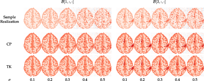
Refer to caption
(a)
Refer to caption
(b)
Refer to caption
(c)
Figure S3: The top block displays the modified Hoffman’s phantom [73] that formed our true \mathcal{B} in the experiments of Section S4. The second block displays a sample realization (first row) and the ^^\mathcal{\widehat{B}} (left block corresponds to the first layer of \mathcal{B}, right block corresponds to the second later of of \mathcal{B}) using the CP (second row) and TK (third row) formats, with optimal ranks estimated by BIC, for σ=0.1,0.2,0.3,0.4,0.5𝜎0.10.20.30.40.5\sigma=0.1,0.2,0.3,0.4,0.5, with data generated having modest AR(1) correlations: ρ1=0.25,ρ2=0.35formulae-sequencesubscript𝜌10.25subscript𝜌20.35\rho_{1}=0.25,\rho_{2}=0.35. The bottom block is similar to the middle block, but it displays performance in the high AR(1) correlations case: here, ρ1=0.6,ρ2=0.8.formulae-sequencesubscript𝜌10.6subscript𝜌20.8\rho_{1}=0.6,\rho_{2}=0.8. We see that although increasing variance and AR(1) correlation lead to noisier sample realizations and parameter estimates, the anatomy of brain structure, and the activation is largely recovered by both formats, even when we have only three realizations under each setting.

S4 Supplement to Section V

[28] recently reported blocking behavior in the direction of the modes of \mathcal{B} when estimating it via low-rank CP and TK formats and in the context of a scalar-on-tensor regression framework. We provide a limited evaluation to see if this behavior is also exhibited in ToTR, for instance, in imaging applications, when we use BIC to tune the ranks. Our evaluation is in the context of the balanced TANOVA(1,2) model

Yi=𝒙i|+Ei,Eiiid𝒩[61,76](0,σ2,Σ1,Σ2),subscript𝑌𝑖inner-productsubscript𝒙𝑖subscript𝐸𝑖subscript𝐸𝑖𝑖𝑖𝑑similar-tosubscript𝒩superscript61760superscript𝜎2subscriptΣ1subscriptΣ2Y_{i}=\langle\bm{x}_{i}|\mathcal{B}\rangle+E_{i},\quad E_{i}\overset{iid}{\sim}\operatorname{\mathcal{N}}_{[61,76]^{\prime}}(0,\sigma^{2},\Sigma_{1},\Sigma_{2}),

with \mathcal{B} being a 3-way tensor of size 2×61×76261762\times 61\times 76, which we chose from the inner 61×76617661\times 76 portion (eliminating all rows and columns consisting only of background pixels) of the 128×128128128128\times 128 digitized Hoffman phantom of [95] and recently adapted by [73] for use in fMRI simulation experiments. The original phantom [95] is a digitized representation of the brain, and the inner (61×76617661\times 76) portion of this phantom formed the first layer (i.e., [1,:,:]1::\mathcal{B}[1,:,:]) of our \mathcal{B}, with the background pixels having value 0, the light foreground pixels having value 1 and the darker foreground pixels having value 2. The second layer [2,:,:]2::\mathcal{B}[2,:,:] had the same values as [1,:,:]1::\mathcal{B}[1,:,:], except for the 138 “truly activated pixels” in two disjoint regions that were introduced by [73] to evaluate activation detection methods in simulation settings. At these pixels, [2,:,:]2::\mathcal{B}[2,:,:] had the value 3. (Fig. S3, top block, displays the two layers of \mathcal{B}.) The vector 𝒙isubscript𝒙𝑖\bm{x}_{i} (where i=1,2,,6𝑖126i=1,2,\dots,6) is a 2D binary vector that indicates which of the two phantom images corresponds to 𝔼(Yi)𝔼subscript𝑌𝑖\mathbb{E}(Y_{i}). We let (Σ1,Σ2)subscriptΣ1subscriptΣ2(\Sigma_{1},\Sigma_{2}) be AR(1) correlation matrices with coefficients (ρ1,ρ2){(0.25,0.35),(0.6,0.8)}subscript𝜌1subscript𝜌20.250.350.60.8(\rho_{1},\rho_{2})\in\{(0.25,0.35),(0.6,0.8)\} to represent cases with low and high correlations among the errors and set σ{0.2,0.4,0.6,0.8,1}𝜎0.20.40.60.81\sigma\in\{0.2,0.4,0.6,0.8,1\}, for five different noise settings.

Fig. S3 (top row of middle and bottom blocks) shows sample realizations of the model under lower (middle block) and high correlations (bottom block) cases. We estimated \mathcal{B} assuming CP and TK formats, with ranks tuned using BIC, as per Section II-E, and displayed these ^^\mathcal{\widehat{B}}s in the second and third rows of the middle and lower blocks of Fig. S3. These estimates show good recovery in \mathcal{B} in all cases, of both the putative anatomical and activation regions, even though it is understandable that this performance depreciates with higher noise and intra-brain correlation coefficients. Lower σ𝜎\sigmas yield larger optimal ranks for both TK and CP, while increasing the AR(1) coefficients increases the model complexity. The figures also indicate that there is not much appreciable blocking effect in the direction of the modes of the tensor. We however, observed blocking behavior, earlier with the CP and TK (and also TR) formats when the ranks were set (see Fig. 7), but not when we allowed BIC to choose these ranks. We also did not observe such patterns with the TR format and BIC-tuned ranks in Fig. 9, even though we achieved a parameter reduction of over 99%. Therefore, while further investigations are needed, our initial evaluations here show that our BIC-optimized reduced-rank (CP and TK) format ToTR and TANOVA do not induce unwanted directional effects, therefore showing promise in imaging and other applications.

References

  • [1] R. A. Johnson and D. W. Wichern, Applied multivariate statistical analysis.   Pearson, 2008.
  • [2] R. Tibshirani, “Regression Shrinkage and Selection Via the Lasso,” Journal of the Royal Statistical Society: Series B (Methodological), vol. 58, no. 1, pp. 267–288, Jan. 1996.
  • [3] J. Friedman, T. Hastie, and R. Tibshirani, “Sparse inverse covariance estimation with the graphical lasso,” Biostatistics, vol. 9, no. 3, pp. 432–441, Jul. 2008.
  • [4] R. D. Cook, B. Li, and F. Chiaromonte, “Envelope models for parsimonious and efficient multivariate liner regression,” Statistica Sinica, vol. 20, no. 3, pp. 927–960, 2010.
  • [5] A. Mukherjee and J. Zhu, “Reduced rank ridge regression and its kernel extensions,” Statistical Analysis and Data Mining, vol. 4, no. 6, pp. 612–622, Dec. 2011.
  • [6] K. A. Busch, J. Fawcett, and D. G. Jacobs, “Clinical correlates of inpatient suicide,” journal of clinical psychiatry, vol. 64, 2003.
  • [7] M. A. Just, L. Pan, V. L. Cherkassky, D. McMakin, C. Cha, M. K. Nock, and D. Brent, “Machine learning of neural representations of suicide and emotion concepts identifies suicidal youth,” Nature Human Behaviour, vol. 1, pp. 911–919, 2017.
  • [8] G. B. Huang, M. Ramesh, T. Berg, and E. Learned-Miller, “Labeled faces in the wild: A database for studying face recognition in unconstrained environments,” University of Massachusetts, Amherst, Tech. Rep., October 2007.
  • [9] M. Afifi and A. Abdelhamed, “Afif4: Deep gender classification based on adaboost-based fusion of isolated facial features and foggy faces,” Journal of Visual Communication and Image Representation, vol. 62, pp. 77 – 86, 2019.
  • [10] N. Kumar, A. C. Berg, P. N. Belhumeur, and S. K. Nayar, “Attribute and simile classifiers for face verification,” in 2009 IEEE 12th International Conference on Computer Vision, Sep. 2009, pp. 365–372.
  • [11] X. Bi, X. Tang, Y. Yuan, Y. Zhang, and A. Qu, “Tensors in statistics,” Annual Review of Statistics and Its Application, vol. 8, no. 1, pp. 345–368, 2021.
  • [12] Y. Panagakis, J. Kossaifi, G. G. Chrysos, J. Oldfield, M. A. Nicolaou, A. Anandkumar, and S. Zafeiriou, “Tensor methods in computer vision and deep learning,” Proceedings of the IEEE, vol. 109, no. 5, pp. 863–890, 2021.
  • [13] P. Hoff, “Multilinear tensor regression for longitudinal relational data,” The Annals of Applied Statistics, vol. 9, 11 2014.
  • [14] W. W. Sun and L. Li, “STORE: sparse tensor response regression and neuroimaging analysis,” The Journal of Machine Learning Research, vol. 18, no. 1, pp. 4908–4944, Jan. 2017.
  • [15] L. Li and X. Zhang, “Parsimonious tensor response regression,” Journal of the American Statistical Association, vol. 112, no. 519, pp. 1131–1146, 2017.
  • [16] W. Guo, I. Kotsia, and I. Patras, “Tensor learning for regression,” IEEE Transactions on Image Processing, vol. 21, no. 2, pp. 816–827, 2012.
  • [17] Y. Fu, J. Gao, X. Hong, and D. Tien, “Tensor regression based on linked multiway parameter analysis,” in 2014 IEEE International Conference on Data Mining, 2014, pp. 821–826.
  • [18] H. Zhou, L. Li, and H. Zhu, “Tensor regression with applications in neuroimaging data analysis,” Journal of the American Statistical Association, vol. 108, no. 502, pp. 540–552, 12 2013.
  • [19] X. Li, H. Zhou, and L. Li, “Tucker tensor regression and neuroimaging analysis,” Statistics in Biosciences, Mar 2018.
  • [20] C. Li and H. Zhang, “Tensor quantile regression with application to association between neuroimages and human intelligence,” Annals of Applied Statistics, vol. 15, no. 3, pp. 1455–1477, 2021.
  • [21] G. Rabusseau and H. Kadri, “Low-Rank Regression with Tensor Responses,” Advances in Neural Information Processing Systems, no. 29, p. 15, 2016.
  • [22] R. Guhaniyogi, S. Qamar, and D. B. Dunson, “Bayesian tensor regression,” Journal of Machine Learning Research, vol. 18, no. 79, pp. 1–31, 2017.
  • [23] T. Ahmed, H. Raja, and W. U. Bajwa, “Tensor regression using low-rank and sparse tucker decompositions,” SIAM Journal on Mathematics of Data Science, vol. 2, no. 4, pp. 944–966, 2020.
  • [24] D. Kong, B. An, J. Zhang, and H. Zhu, “L2rm: Low-rank linear regression models for high-dimensional matrix responses,” Journal of the American Statistical Association, vol. 115, no. 529, pp. 403–424, 2020.
  • [25] Y. Zhou, R. K. W. Wong, and K. He, “Tensor Linear Regression: Degeneracy and Solution,” IEEE Access, vol. 9, 2021.
  • [26] Y. Deng, X. Tang, and A. Qu, “Correlation tensor decomposition and its application in spatial imaging data,” Journal of the American Statistical Association, vol. 0, no. 0, pp. 1–17, 2021.
  • [27] J. C. Poythress, J. Ahn, and C. Park, “Low-rank, orthogonally decomposable tensor regression with application to visual stimulus decoding of fmri data,” Journal of Computational and Graphical Statistics, vol. 0, no. 0, pp. 1–14, 2021.
  • [28] G. Papadogeorgou, Z. Zhang, and D. B. Dunson, “Soft tensor regression,” Journal of Machine Learning Research, vol. 22, no. 219, pp. 1–53, 2021. [Online]. Available: http://jmlr.org/papers/v22/20-476.html
  • [29] E. Lock, “Tensor-on-tensor regression,” Journal of Computational and Graphical Statistics, 01 2017.
  • [30] J. D. Carroll and J.-J. Chang, “Analysis of individual differences in multidimensional scaling via an n-way generalization of “Eckart-Young” decomposition,” Psychometrika, vol. 35, no. 3, 1970.
  • [31] R. A. Harshman, “Foundations of the parafac procedure: Models and conditions for an explanatory” multi-modal factor analysis,” UCLA Working Papers in Phonetics, no. 16, 1970.
  • [32] Y. Liu, J. Liu, and C. Zhu, “Low-Rank Tensor Train Coefficient Array Estimation for Tensor-on-Tensor Regression,” IEEE Transactions on Neural Networks and Learning Systems, vol. 31, Dec. 2020.
  • [33] C. Llosa, “Tensor on tensor regression with tensor normal errors and tensor network states on the regression parameter,” Iowa State University Creative Components, vol. 82, Jan. 2018. [Online]. Available: https://lib.dr.iastate.edu/creativecomponents/82
  • [34] W. Zhao, K. M. Kendrick, F. Chen, H. Li, and T. Feng, “Neural circuitry involved in quitting after repeated failures: role of the cingulate and temporal parietal junction,” Scientific Reports, vol. 6, no. 1, p. 24713, Apr. 2016.
  • [35] I. Oseledets, “Tensor-train decomposition,” SIAM Journal on Scientific Computing, vol. 33, no. 5, pp. 2295–2317, 2011.
  • [36] G. Brandi and T. Di Matteo, “Predicting multidimensional data via tensor learning,” Journal of Computational Science, vol. 53, p. 101372, 2021.
  • [37] L. R. Tucker, “Some mathematical notes on three-mode factor analysis,” Psychometrika, vol. 31, no. 3, pp. 279–311, Sep 1966.
  • [38] T. G. Kolda and B. W. Bader, “Tensor decompositions and applications,” SIAM Review, vol. 51, no. 3, pp. 455–500, September 2009.
  • [39] M. Bahri, Y. Panagakis, and S. Zafeiriou, “Robust Kronecker-Decomposable Component Analysis for Low-Rank Modeling,” in 2017 IEEE International Conference on Computer Vision (ICCV), Oct. 2017, pp. 3372–3381.
  • [40] P. Hoff, “Separable covariance arrays via the tucker product, with applications to multivariate relational data,” Bayesian Analysis, vol. 6, no. 2, pp. 179–196, 06 2011.
  • [41] D. Akdemir and A. Gupta, “Array variate random variables with multiway kronecker delta covariance matrix structure,” Journal of Algebraic Statistics, vol. 2, pp. 98–113, 01 2011.
  • [42] M. Ohlson, M. R. Ahmad, and D. von Rosen, “The multilinear normal distribution: Introduction and some basic properties,” Journal of Multivariate Analysis, vol. 113, pp. 37 – 47, 2013.
  • [43] A. M. Manceur and P. Dutilleul, “Maximum likelihood estimation for the tensor normal distribution: Algorithm, minimum sample size, and empirical bias and dispersion,” Journal of Computational and Applied Mathematics, vol. 239, pp. 37 – 49, 2013.
  • [44] T. G. Kolda, “Multilinear operators for higher-order decompositions.” Sandia National Laboratories, Tech. Rep. SAND2006-2081, 923081, Apr. 2006.
  • [45] A. Cichocki, N. Lee, I. Oseledets, A.-H. Phan, Q. Zhao, and D. P. Mandic, “Tensor networks for dimensionality reduction and large-scale optimization: Part 1 low-rank tensor decompositions,” Foundations and Trends® in Machine Learning, vol. 9, no. 4-5, 2016.
  • [46] L. De Lathauwer, B. De Moor, and J. Vandewalle, “A multilinear singular value decomposition,” SIAM Journal on Matrix Analysis and Applications, vol. 21, no. 4, pp. 1253–1278, 2000.
  • [47] D. Gerard and P. Hoff, “A higher-order LQ decomposition for separable covariance models,” Linear Algebra and its Applications, vol. 505, pp. 57 – 84, 2016.
  • [48] R. Orús, “A practical introduction to tensor networks: Matrix product states and projected entangled pair states,” Annals of Physics, vol. 349, pp. 117 – 158, 2014.
  • [49] G. Z. Thompson, R. Maitra, W. Q. Meeker, and A. F. Bastawros, “Classification With the Matrix-Variate-t Distribution,” Journal of Computational and Graphical Statistics, vol. 29, no. 3, Jul. 2020.
  • [50] A. Gupta and D. Nagar, Matrix Variate Distributions.   Taylor & Francis, 1999.
  • [51] M. M. Wolf, F. Verstraete, M. B. Hastings, and J. I. Cirac, “Area laws in quantum systems: Mutual information and correlations,” Physical review letters, vol. 100, p. 070502, 03 2008.
  • [52] M. S. Srivastava, T. von Rosen, and D. von Rosen, “Models with a kronecker product covariance structure: Estimation and testing,” Mathematical Methods of Statistics, vol. 17, no. 4, Dec 2008.
  • [53] J. de Leeuw, “Block-relaxation algorithms in statistics,” in Information Systems and Data Analysis.   Berlin, Heidelberg: Springer Berlin Heidelberg, 1994, pp. 308–324.
  • [54] H. Abdi, “Singular value decomposition (svd) and generalized singular value decomposition (gsvd),” Encyclopedia of Measurement and Statistics., 01 2007.
  • [55] H. Glanz and L. Carvalho, “An expectation maximization algorithm for the matrix normal distribution with an application in remote sensing,” Journal of Multivariate Analysis, vol. 167, 2018.
  • [56] C. Viroli, “On matrix-variate regression analysis,” Journal of Multivariate Analysis, vol. 111, pp. 296 – 309, 2012.
  • [57] S. Ding and R. Cook, “Matrix-variate regressions and envelope models,” Journal of the Royal Statistical Society: Series B (Statistical Methodology), vol. 80, 05 2016.
  • [58] W. Hackbusch and S. Kühn, “A new scheme for the tensor representation,” Journal of Fourier Analysis and Applications, vol. 15, pp. 706–722, 10 2009.
  • [59] L. Grasedyck, “Hierarchical singular value decomposition of tensors,” SIAM Journal on Matrix Analysis and Applications, vol. 31, no. 4, pp. 2029–2054, 2010.
  • [60] I. D. Currie, M. Durban, and P. H. C. Eilers, “Generalized Linear Array Models with Applications to Multidimensional Smoothing,” Journal of the Royal Statistical Society. Series B (Statistical Methodology), vol. 68, no. 2, pp. 259–280, 2006.
  • [61] R. Kashyap, “A bayesian comparison of different classes of dynamic models using empirical data,” IEEE Transactions on Automatic Control, vol. 22, no. 5, pp. 715–727, 1977.
  • [62] G. Schwarz, “Estimating the dimension of a model,” Ann. Statist., vol. 6, no. 2, pp. 461–464, 03 1978.
  • [63] K. V. Mardia, J. T. Kent, and J. M. Bibby, Multivariate analysis.   New York: Academic Press, 1979.
  • [64] R. Heller, D. Stanley, D. Yekutieli, N. Rubin, and Y. Benjamini, “Cluster-based analysis of fMRI data,” NeuroImage, vol. 33, no. 2, pp. 599–608, nov 2006.
  • [65] R. W. Cox, “AFNI: software for analysis and visualization of functional magnetic resonance neuroimages,” Computers and Biomedical research, vol. 29, no. 3, pp. 162–173, 1996.
  • [66] R. W. Cox and J. S. Hyde, “Software tools for analysis and visualization of fMRI data,” NMR in Biomedicine, vol. 10, no. 4-5, pp. 171–178, 1997.
  • [67] C. R. Genovese, N. A. Lazar, and T. Nichols, “Thresholding of statistical maps in functional neuroimaging using the false discovery rate,” Neuroimage, vol. 15, pp. 870–878, 2002.
  • [68] Y. Benjamini and R. Heller, “False discovery rates for spatial signals,” Journal of the American Statistical Association, vol. 102, no. 480, pp. 1272–1281, 2007.
  • [69] M. Smith and L. Fahrmeir, “Spatial Bayesian variable selection with application to functional Magnetic Resonance Imaging,” Journal of the American Statistical Association, vol. 102, no. 478, pp. 417–431, 2007.
  • [70] S. M. Smith and T. E. Nichols, “Threshold-free cluster enhancement: Addressing problems of smoothing, threshold dependence and localisation in cluster inference,” Neuroimage, vol. 44, 2009.
  • [71] K. Tabelow, J. Polzehl, H. U. Voss, and V. Spokoiny, “Analyzing fMRIexperiments with structural adaptive smoothing procedures,” NeuroImage, vol. 33, no. 1, pp. 55–62, 2006.
  • [72] J. Polzehl, H. U. Voss, and K. Tabelow, “Structural adaptive segmentation for statistical parametric mapping,” NeuroImage, vol. 52, no. 2, pp. 515–523, 2010.
  • [73] I. A. Almodóvar-Rivera and R. Maitra, “FAST adaptive smoothed thresholding for improved activation detection in low-signal fMRI,” IEEE Transactions on Medical Imaging, vol. 38, no. 12, pp. 2821–2828, 2019.
  • [74] W. Cheng, E. T. Rolls, J. Qiu, D. Yang, H. Ruan, D. Wei, L. Zhao, J. Meng, P. Xie, and J. Feng, “Functional Connectivity of the Precuneus in Unmedicated Patients With Depression,” Biological Psychiatry: Cognitive Neuroscience and Neuroimaging, vol. 3, no. 12, pp. 1040–1049, Dec. 2018.
  • [75] Y. Jacob, L. S. Morris, K.-H. Huang, M. Schneider, S. Rutter, G. Verma, J. W. Murrough, and P. Balchandani, “Neural correlates of rumination in major depressive disorder: A brain network analysis,” NeuroImage: Clinical, vol. 25, p. 102142, Jan. 2020.
  • [76] H.-X. Zhou, X. Chen, Y.-Q. Shen, L. Li, N.-X. Chen, Z.-C. Zhu, F. X. Castellanos, and C.-G. Yan, “Rumination and the default mode network: Meta-analysis of brain imaging studies and implications for depression,” NeuroImage, vol. 206, p. 116287, Feb. 2020.
  • [77] A. Bechara, H. Damasio, and A. R. Damasio, “Emotion, Decision Making and the Orbitofrontal Cortex,” Cerebral Cortex, vol. 10, no. 3, pp. 295–307, Mar. 2000.
  • [78] F. Jollant, N. S. Lawrence, V. Giampietro, M. J. Brammer, M. A. Fullana, D. Drapier, P. Courtet, and M. L. Phillips, “Orbitofrontal cortex response to angry faces in men with histories of suicide attempts,” The American Journal of Psychiatry, vol. 165, no. 6, pp. 740–748, Jun. 2008.
  • [79] A. B. Satpute and K. A. Lindquist, “The Default Mode Network’s Role in Discrete Emotion,” Trends in Cognitive Sciences, vol. 23, no. 10, pp. 851–864, Oct. 2019.
  • [80] S. R. Simon, M. Meunier, L. Piettre, A. M. Berardi, C. M. Segebarth, and D. Boussaoud, “Spatial attention and memory versus motor preparation: premotor cortex involvement as revealed by fMRI,” Journal of Neurophysiology, vol. 88, no. 4, pp. 2047–2057, Oct. 2002.
  • [81] M. Koenigs, A. K. Barbey, B. R. Postle, and J. Grafman, “Superior Parietal Cortex Is Critical for the Manipulation of Information in Working Memory,” Journal of Neuroscience, vol. 29, no. 47, pp. 14 980–14 986, Nov. 2009.
  • [82] J. J. Maller, R. H. S. Thomson, J. V. Rosenfeld, R. Anderson, Z. J. Daskalakis, and P. B. Fitzgerald, “Occipital bending in depression,” Brain, vol. 137, no. 6, pp. 1830–1837, Jun. 2014.
  • [83] R. Smith, R. D. Lane, A. Alkozei, J. Bao, C. Smith, A. Sanova, M. Nettles, and W. D. S. Killgore, “The role of medial prefrontal cortex in the working memory maintenance of one’s own emotional responses,” Scientific Reports, vol. 8, no. 1, p. 3460, Feb. 2018.
  • [84] E. T. Rolls, “The cingulate cortex and limbic systems for action, emotion, and memory,” Handbook of Clinical Neurology, vol. 166, pp. 23–37, 2019.
  • [85] E. J. Bubb, L. Kinnavane, and J. P. Aggleton, “Hippocampal – diencephalic – cingulate networks for memory and emotion: An anatomical guide,” Brain and Neuroscience Advances, vol. 1, 2017.
  • [86] S. R. Heilbronner, B. Y. Hayden, and M. L. Platt, “Decision Salience Signals in Posterior Cingulate Cortex,” Frontiers in Neuroscience, vol. 5, Apr. 2011.
  • [87] Q. Zhao, G. Zhou, S. Xie, L. Zhang, and A. Cichocki, “Tensor ring decomposition,” CoRR, vol. abs/1606.05535, 2016.
  • [88] D. Zaitchik, C. Walker, S. Miller, P. LaViolette, E. Feczko, and B. C. Dickerson, “Mental state attribution and the temporoparietal junction: An fMRI study comparing belief, emotion, and perception,” Neuropsychologia, vol. 48, no. 9, pp. 2528–2536, Jul. 2010.
  • [89] G. Lettieri, G. Handjaras, E. Ricciardi, A. Leo, P. Papale, M. Betta, P. Pietrini, and L. Cecchetti, “Emotionotopy in the human right temporo-parietal cortex,” Nature Communications, vol. 10, no. 1, p. 5568, Dec. 2019.
  • [90] L. G. Ungerleider, S. M. Courtney, and J. V. Haxby, “A neural system for human visual working memory,” Proceedings of the National Academy of Sciences, vol. 95, no. 3, pp. 883–890, Feb. 1998.
  • [91] J. R. Magnus and H. Neudecker, Matrix differential calculus with applications in statistics and econometrics, third edition ed., ser. Wiley series in probability and statistics.   Wiley, 2019.
  • [92] K. B. Petersen and M. S. Pedersen, “The matrix cookbook,” nov 2012, version 20121115.
  • [93] E. L. Lehmann, Elements of large-sample theory, ser. Springer texts in statistics.   New York: Springer, 1999.
  • [94] T.-T. Lu and S.-H. Shiou, “Inverses of 2 x 2 block matrices,” Computers & Mathematics with Applications, vol. 43, no. 1, pp. 119–129, 2002.
  • [95] E. Hoffman, P. Cutler, W. Digby, and J. Mazziotta, “3-d phantom to simulate cerebral blood flow and metabolic images for pet,” IEEE Transactions on Nuclear Science, vol. 37, no. 2, pp. 616–620, 1990.