Time Aggregation Techniques Applied to a Capacity Expansion Model for Real-Life Sector Coupled Energy Systems
Abstract
Simulating energy systems is vital for energy planning to understand the effects of fluctuating renewable energy sources and integration of multiple energy sectors. Capacity expansion is a powerful tool for energy analysts and consists of simulating energy systems with the option of investing in new energy sources. In this paper, we apply clustering based aggregation techniques from the literature to very different real-life sector coupled energy systems. We systematically compare the aggregation techniques with respect to solution quality and simulation time. Furthermore, we propose two new clustering approaches with promising results. We show that the aggregation techniques result in consistent solution time savings between 75% and 90%. Also, the quality of the aggregated solutions is generally very good. To the best of our knowledge, we are the first to analyze and conclude that a weighted representation of clusters is beneficial. Furthermore, to the best of our knowledge, we are the first to recommend a clustering technique with good performance across very different energy systems: the k-means with Euclidean distance measure, clustering days and with weighted selection, where the median, maximum and minimum elements from clusters are selected. A deeper analysis of the results reveal that the aggregation techniques excel when the investment decisions correlate well with the overall behavior of the energy system. We propose future research directions to remedy when this is not the case.
Keywords: Capacity expansion; energy system models; time aggregation; clustering; solution time reduction
1 Introduction
Simulating energy systems is vital for energy planning. The green transition demands increasing introduction of fluctuating renewable energy sources and integration of multiple energy sectors. Simulations are necessary to understand the behavior in such sector coupled energy systems. Capacity expansion consists of simulating energy systems with the option of investing in energy sources. This is a very powerful tool to understand the effects of new technologies.
A tremendous amount of work in the literature considers solution methods for the capacity expansion problems but focuses on single methods or specific energy systems, see e.g. [8, 9, 3, 44]. The contribution of this paper is to recommend a solution approach with overall good performance. It does so by comparing existing and new solution methods on very different energy systems. This differs from the more common approach from the literature of solving the capacity expansion problem for specific energy systems to perfection. This is further elaborated in the literature review.
In this paper, a capacity extension model consists of a year in one-hour resolution, i.e. of 8760 hours. The underlying energy system may consist of many areas (e.g. geographical areas or spot market bidding zones) and energy types (e.g. power, district heating, gas), which results in large capacity extension models. Solving the NP-hard capacity expansion problem is thus time consuming and at times even intractable. Aggregating time steps is a common method to simplify simulations to reach tractability. The literature suggests a wide variety of aggregation techniques. Many studies, however, consider specific systems [3] and only few contributions compare their results with the literature [9].
The novelty of our work lies in analyzing the effect of time aggregation methods on the real-life sector coupled energy systems. To the best of our knowledge, we are the first to apply and compare multiple time aggregation methods on significantly different energy systems. This provides much insight in the potential of time aggregation techniques without the risk of overfitting the methods to specific energy systems. Furthermore, we propose two new aggregation methods with promising results. All time aggregation techniques are based on clustering. We analyze methods for selecting cluster representatives and conclude that weighted selection has superior performance. Finally, we provide a deeper analysis of the achieved results to highlight interesting future research areas in time aggregation techniques. The paper addresses gaps in the current literature of time aggregation techniques applied to capacity expansion models: comparison of methods on very different energy systems, and analysis of selection strategies in the clustering methods.
The paper is structured as follows. The literature review in Section 2 introduces the capacity expansion problem, considers aggregation techniques from the literature and concludes with a motivation for the contributions of this paper. The considered aggregation techniques are presented in Section 3 and the real-life energy systems in Section 4. The clustering methods are evaluated on the energy systems in Section 5. The evaluation leads to the proposal of two new aggregation techniques in Section 5.4. Section 6 contains a discussion of lessons learned and of possible future work. Finally, conclusions are drawn in Section 7.
2 Literature review
The literature review first focuses on the capacity expansion problem and afterwards on solution methods for the capacity expansion problem.
2.1 The Capacity Expansion Problem
We first consider the Unit Commitment Problem (UC) and then the Capacity Expansion Problem (CEP). The importance of considering the UC together with the CEP has been quantified in several studies, which show that ignoring the operation details from the UC leads to underestimations in flexibility measures and overestimation of base-load and renewable energy sources (RES) [34, 21, 12].
The Unit Commitment Problem simulates an energy system, where demand must be met every hour [4]. It determines the operation schedule of generating units, subject to demand, technical constraints, available RES, etc [31]. It is NP-hard and includes binary decision variables for turning production units on and off [7]. A general mathematical model for the unit commitment problem can be summarized as:
| min | total system costs | (1) | ||
| s.t. | production + import + storage discharge = demand + export + storage charge | (2) | ||
| physical constraints on production units | (3) | |||
| available RES | (4) | |||
| storage and electric vehicle constraints | (5) | |||
| capacity on interconnection lines | (6) |
The total system costs (1) include fuel prices, costs on production and fuel consumption (e.g. taxes, subsidies), emission costs, import and export costs, operation and management costs, startup costs and costs associated with flexible demands. Balance constraints (2) ensure that supply and demand meet in every area and in every hour. Supply consists of production, import and storage discharge. Demand consist of demand, export and storage discharge. Balance constraints include slack variables, which are activated when demand and supply cannot be matched. Physical constraints on production units (3) include unit commitment, fuel consumption, efficiency, startup costs, technical production limits, production technology (condensation, back pressure, extraction, turbine bypass, heat boiler, etc.) and ramping. Constraints (4) consider available RES subject to curtailment options. Storage and electric vehicle constraints (5) include capacities, losses, charge and discharge rates, and, for electric vehicles, charging before driving. Finally, (6) ensure that capacities on interconnection lines are satisfied.
The UC is subject to a considerable amount of research in order to increase the tractability of the problem by e.g. linearizing non-linear constraints [51], reducing the number of binary variables [10], tightening the formulation [37], applying dynamic programming solution methods, heuristics and math-heuristics, see [31] for a survey and comparison of methods.
The Capacity Expansion Problem (CEP) extends the Unit Commitment Problem with investment decisions. This enables analyses of introduction of new technologies, energy mix in case of rapid technology development, flexibility needs, etc. [9]. A general mathematical model for the CEP is summarized as:
| min | total system costs + investment costs | (7) | ||
| s.t. | production + import + storage discharge = demand + export + storage charge | (8) | ||
| physical constraints on production units | (9) | |||
| available RES | (10) | |||
| storage and electric vehicle constraints | (11) | |||
| capacity on interconnection lines | (12) | |||
| utilization investment | (13) | |||
| min investment investment max investment | (14) |
The objective function (7) ensures that an investment takes place when the savings of utilizing the investment exceed the investment cost. “Utilization” in constraints (13) represents how the investment is utilized in terms of production (for production units and RES), inventory level (for storage units) or import and export (for interconnection lines). The constraints say that the investment must be large enough to facilitate the desired utilization. Finally, bounds (14) ensure that investments are within the user defined bounds.
The CEP is widely used for optimizing the configuration of future energy systems. Examples of applications are non-trivial power systems [25], integration of renewable energy [36], large energy systems with sector coupling such as power, gas, transport and heating [8], and the impact of scenarios [53]. An important type of CEP is the Generation Expansion Planning (GEP) which considers electricity systems [3]. The GEP optimizes the capacities and can give input to locations and commissioning times, see [36, 24, 44, 11] for reviews and for applications on different energy systems.
As mentioned, incorporating the UC in the CEP is essential to analyse the need for flexibility capacities and the integration of RES [34, 21, 12]. This is particularly the case in systems with much RES [47, 38] or when alternative flexibility sources are analysed [41]. Recall that the UC is NP-hard. Several studies have thus considered simplified approaches to include the UC in the CEP [21, 10, 37, 51], e.g., by only considering a subset of the UC constraints [23, 6, 52, 42], however, the resulting problem still remains very difficult to solve. Further research has looked into sophisticated solution approaches such as Benders decomposition [45] and Dantzig-Wolfe decomposition [16]. A very popular approach is time aggregation, where only a subset of the 8760 hours of the year is solved. This reduces the size of the problem to make it more tractable, but at the cost of losing precision. Several literature studies apply different sophisticated strategies to select a subset of the 8760 hours and conclude that the quality is satisfying, see e.g. [25, 49, 39, 40, 46]. The next section further elaborates time selection methods.
2.2 Time aggregation techniques for the Capacity Expansion Problem
Many different time aggregation techniques exist, spanning from simple heuristic selections [17] to optimization methods [40]. Heuristic approaches may be too simple and are at times associated with insufficient capture of variability [32] while the optimization approaches suffer from high computational efforts [40]. It seems that a good compromise between quality and computational tractability is achieved by using clustering procedures [26, 20, 27, 1]. A survey along with a proposed classification of time aggregation methods can be found in [9].
In this article, we focus on clustering methods. This literature study first reviews literature on clustering methods, then on how to select elements from clusters, then on comparing methods and finally we discuss how this paper contributes to closing gaps in the literature.
2.2.1 Clustering techniques
The aim of all clustering approaches is to minimize the similarity between clusters while maximizing the similarity within each cluster [15]. Clustering approaches differ in how they group elements into clusters and how they select elements from each cluster. An example of a clustering technique can be found in [33], which clusters days according to the hierarchical clustering procedure and where the day closest to each cluster centroid is chosen. Other popular approaches are k-means [30] and fuzzy clustering [13].
Clustering techniques can be categorized into either Exclusive (each element is assigned to only one cluster) or overlapping cluster techniques (each element is assigned to all clusters with a degree of membership) [9]. In relation to time aggregation, most clustering approaches belong to the Exclusive category, although the use of some overlapping clustering techniques, such as a fuzzy clustering, also exists [9, 14, 28]. The most common Exclusive techniques are the Hierarchical clustering and the k-means clustering; the former builds a hierarchy of clusters through a sequence of nested partitions, while the latter initializes a grouping which is then iteratively improved [19].
2.2.2 Selecting elements from clusters
The hypothesis of using clustering techniques for time aggregation is that the resulting selected elements include all information needed to make optimal investments. However, perfect similarity within the clusters is usually not achieved, wherefore the strategy of selecting elements from each cluster influences the aggregation performance. The authors of [18] provide an overview of selection strategies including cluster average, element closest to the cluster average and random element selection. Average representatives are frequently criticized for smoothing the profiles [35, 39] with a consequence of underestimating the need for storage capacity and storage technologies [22]. On the other hand, a random selection shows good results in [9] where also both minimum and maximum element selections are included in the comparison. Apart from [9], comparisons of element selections are seen in [33] and [14]. After the selection, the elements are weighted such that the aggregation reflects the relative importance of the elements in the original problem. Typically, fixed weighting is applied, assuming each cluster element to be equally important [28]. The weighting could also choose only to represent a partition of the clusters [43]. To our knowledge, there is no clear conclusion regarding the existence of a single best selection criteria nor a single best weighting strategy.
2.2.3 Comparison of aggregation methods
Relatively few articles in the literature compare clustering methods systematically. In the following, we bring forward some of the more interesting contributions. [5] compare clustering procedures, which group days into clusters. Only single clustering techniques are considered and each clustering uses a similarity metric based on the principle components of the day elements. The clustering procedures are the k-means, the fuzzy cmean clustering and hierarchical clustering with varying linkage criteria. Two different element selections strategies are considered; the mean and the median element selection. In both cases, the selected element is weighted (repeated) according to the number of elements in its cluster. The paper analyzes electricity demand only, and furthermore it only considers how well the original data is represented by the clustering. It does not consider the quality with respect to the investment results. Based on the input data considerations, they conclude that the k-means clustering using median representative outperforms other clustering procedures, independently of the number of clusters.
In [28], different clustering based aggregation techniques each selecting days are also compared. Demand, solar and wind timeseries are considered in the aggregation, each normalized such that they are equally important in the aggregation. Three aggregation techniques are considered. A hierarchical clustering with a minmax linkage criterion and a dynamic time wrapping distance metric. A double clustering strategy first applying a k-means clustering, followed by a re-clustering using the aforementioned hierarchical procedure. The last technique is a pure k-means clustering. Each aggregated timeseries consists of 30 selected days, and the comparison is based on test runs in a capacity expansion model assuming continuous investment decisions and without unit commitment decisions. The case study is based on a single dataset covering three regions. The aggregation methods are compared on their ability to replicate investments, which are possible in wind, solar, coal, natural gas, nuclear and a generic storage technology. The mean element is selected from each cluster, and selected elements are weighted (repeated) according to the number of elements in the clusters. They conclude that the hierarchical clustering and the double clustering have similar performance, which is better than the one obtained for a k-means clustering.
In [50], five different day selecting clustering approaches are compared. First, a k-means and a k-medoids clustering each based on an Euclidean distance metric and cluster centers as representative elements. Then, a dynamic time warping barycenter averaging clustering, a k-shape clustering with a shape-based distance metric and lastly, a hierarchical clustering with Euclidean distance metric and medoid element as cluster representative. Only price timeseries are considered for the aggregation and each timeseries is normalized (daily) using a z-normalization. Each clustering procedure is considered for 1-9 clusters, but the quality of the approaches is measured only by comparing the selected data to the original data, i.e. in a data validation framework [9]. After having decided on the number of clusters, the techniques are compared based on their resulting investments. The comparison is based on two different MIP models representing different energy systems: one based on an electricity storage and one based on a gas turbine power generation. Furthermore, each aggregation is applied to each system for two different timeseries of electricity prices. They conclude that the centroid-based clusterings better replicate the operational part while they also tend to underestimate objective values compared to the medoid-based approaches.
In [9], three clustering procedures are compared to four non-clustering aggregation techniques. The procedures are carefully selected from the literature to represent classes of proposed methods. Also, three new aggregation techniques are proposed; one based on dynamically blocking days, one based on optimizing the statistical representation of selected days; and one based on double clustering including correlation as distance measure. All methods are compared on three test instances inspired by the Danish power system and with different amounts of RES. The goal of the study is a broader comparison of methods to provide general insight in the performance of aggregation techniques. A conclusion from the study is that even though a double clustering procedure is concluded to provide overall best performance, the much simpler aggregation approaches show to be strong competitors.
2.3 Hypothesis and contribution of this paper
The common approach in the literature is to solve specific energy systems, which makes it difficult to compare the results. [5] conclude that k-means has best performance, [28] hierarchical and double clustering, in [50] medoid based selection is best for investment decisions and [9] show that simple heuristic based aggregation approaches perform well. In [50] they do compare across different energy systems, but these energy systems are based on different underlying MIPs which again makes it difficult to draw conclusions for the CEP.
A similar pattern can be seen for element selection strategy. Comparisons of different selection criteria is not common in the literature. Exceptions are [14] considering median and mean representatives with median as best option, [33] considering selection of centroid or historical day representation with centroid as best option, and [9] considering minimum, maximum, mean and random element selections with random as best option.
Moreover, to our knowledge, the question of selecting
multiple elements from each cluster has not been addressed until the
current paper. In both [14] and [28], the cluster
representative is weighted according to the cluster sizes, however
without argumentation nor analysis of why. To the best of our
understanding, weighting is performed by repeating each cluster
representative instead of selecting multiple elements from the
clusters.
A different view on solving problems can be taken from the research field of optimizing solvers. Here, the goal is not to solve each problem to perfection, but to find an approach, which provides overall good performance among different problems [2]. This is also the focus of this paper.
The main contribution of this paper is a detailed and structured comparison of different time aggregation approaches on four very different energy systems, based on the same mathematical formulation. With the energy systems being realistic in size and detail, the conclusions are widely applicable. Since the aggregation technique comparison also includes a very simple approach, this paper furthermore illuminates the relation between aggregation technique complexity and performance. The paper further contributes by comparing different selection strategies when elements are to be selected from each cluster and by considering both single and multiple selections from each cluster. Also, to the best of our knowledge, this paper is the first to illustrate the benefits of considering clustering weightings in the selection.
This paper focuses on the energy simulation model, Sifre. The full mathematical formulation of Sifre is available at [48] and the capacity expansion module of Sifre is available in Appendix A. Investment decisions are supported for production units, renewable units, storage, electric vehicles and interconnection lines.
When solving the investment problem, a full year is simulated. Sifre LP relaxes the problem to limit the simulation solution time. The integer variables in the unit commitment problem are LP relaxed and investments are linear instead of discrete (e.g. invest between 0 and 500 MW in a production unit, instead of investing in zero, one or two production units, each of size 150 MW). Still, solving the problem may take many hours because of the problem instance size.
3 Solution methods
Numerous aggregation approaches are suggested in the literature. Buchholz et al. [9] survey the many approaches and computationally compare aggregation strategies from the literature. According to their studies, the following approaches show superior performance:
-
•
Dummy Selection, where every 13th element is selected from the residual load curve
-
•
Statistical Representation, which selects 10000 random samples and from this select the sample that best represents the means and standard deviation of the original data
-
•
Optimized Selection, which has same objective as Statistical Representation. Instead of investigating 10000 random samples, this approach finds the optimal sample with respect to means and standard deviation of the original data
-
•
k-means Clustering with squared Euclidean distance measurement
-
•
Cluster Clustering which first applies k-means clustering with squared Euclidean distances. Each resulting cluster is re-clustered using hierarchical agglomerative clustering with dynamic time warp distance measure and complete linkage criterion (minimizes the maximum distance between two elements; one in each cluster)
-
•
Level Correlation Clustering, which first applies fuzzy clustering with squared Euclidean distances. Then it applies hierarchical agglomerative clustering according to element correlations
To scope the work in this paper, we decide to focus on the clustering methods (the three last methods). We also include Dummy Selection due to its simplicity. As the sector coupled energy systems consist of many timeseries (and not just the residual load), we select every 13th element from each timeseries in Dummy Selection.
3.1 Configuration of the clustering approaches
The survey of Buchholz et al. [9] shows promising results when clustering days into 28 clusters. We thus apply this configuration. Both the Cluster Clustering and the Level Correlation Clustering generates 7 outer clusters, each of which are re-clustered into 4 sub clusters.
The k-means clustering and fuzzy clustering algorithms depend on an initial cluster. We divide the simulation period evenly into the number of desired clusters. E.g. consider a year of 365 days, where the number of desired clusters is 28 and where days are clustered. Then the first 13 days are assigned to the first cluster, the next 13 days to the next cluster etc.
3.2 Data dimensions
The proposed methods are extended to handle complex sector coupled energy systems, by making them consider all fluctuating timeseries data. This means that the methods consider demand of all energy types (e.g. power, district heating, gas), RES production, import/export prices, fuel prices and availability profiles for production units and interconnection lines. The clustering approaches consider every fluctuating timeseries separately (instead of summing them into e.g. a residual load curve) and we also maintain the chronological order (in contrast to duration curves). Demand is negated to make the selection of cluster elements more intuitively understandable. The minimum sum element in a cluster represents a day with low production and high demand. Similarly, the maximum sum element represents a day with high production and little demand. The clustering approaches must calculate the distance between two days. This is done for each matching pair of timeseries for each hour (e.g. the RES production by offshore wind park Horns Rev 1 for each of the two days). All differences are summed across hours and timeseries to produce the final distance between the two cluster days.
3.3 Selecting days from clusters
Two approaches can be considered for deciding the number of days to select from each cluster. Either one day from each cluster (denoted non-weighted or fixed weighted), or a weighted number of days from each cluster. The benefit of the latter is that typical days and outliers in the full dataset remain (somewhat) typical and outlying in the aggregated dataset. The weight is set according to the cluster size:
| (15) | |||
| (16) |
The total number of selected days may exceed the number of clusters for weighted selection. Weighted selection in the literature consists of selecting a single element from each cluster and then repeating this element a number of times [33, 14, 28]. We propose to instead select a weighted number of elements from each cluster. The benefit of this is that time chronology is maintained, i.e., once selection of elements has finished, the original order of the selected elements is applied. Also, selecting existing elements instead of generating new, should represent the original data better.
Several strategies are investigated for deciding which days to select from each cluster: Minimum sum, i.e. the day(s) with smallest sum; Maximum sum, i.e. the day(s) with largest sum; Median sum, i.e. the day(s) with median sum; Closest to Cluster Mean, i.e. the day(s) with shortest distance to the cluster mean, and Random i.e. randomly chosen day(s). Closest to Cluster Mean is calculated as follows: The mean of a day is calculated for every hour. The distance from an element to the mean is the total Euclidean distance in the 24-dimensional space.
3.4 Test setup
The time aggregation techniques are compared to the optimal solution of each data instance, i.e. we apply model validation to measure the quality of the aggregation techniques [9]. Since only part of the problem is solved by the time aggregation techniques, the objective function values cannot be compared out of the box. It is, however, possible to generate two full year simulations with fixed investments: one simulation with optimal investments and another simulation with investments from using a time aggregation technique. The objective function values of these two simulations can then be compared. But the objective function values will not include investment costs and will thus be difficult to understand in relation to investment decisions. Also, the objective function value is of very little interest in the analyses in Energinet, where focus is on the energy mix, the flows, etc. For this reason, we decide to only compare the investment decisions. The performance measure hence becomes:
| (17) |
where is an index for the investments, is the investment decision made by the aggregation technique and the investment decision from the optimal solution.
4 Test instances
The aggregation techniques are tested on four significantly different sector coupled energy systems, all stemming from analyses in Energinet. The energy systems are different instances of the LP model summarized in Section 2.1. An energy system consists of the following components:
-
•
Areas, which represent an energy type and a geographical region, possibly attached an energy demand
-
•
External areas represent an energy type and a geographical region. They only have a price per MWh for each hour attached. They can only be connected to the rest of the system via an interconnection line
-
•
Production units (or Conversion units or Generation units) convert energy types; examples are CHPs, CCGTs and compressors,
-
•
Renewable units produce energy based on a production profile
-
•
Storages are any types of storages, e.g., batteries or water tanks. Storages can also be used to model line pack in gas systems
-
•
Electric vehicles which must be charged before requested driving time, however, the time of charging is flexible
The sector coupled energy systems are described in Table 1.
| Energy system | Areas | External areas | Production units | RES |
|---|---|---|---|---|
| DK classic | 74 | 6 | 294 | 60 |
| DK detailed | 211 | 9 | 396 | 88 |
| Gas | 74 | 2 | 70 | 7 |
| PtX | 27 | 8 | 31 | 1 |
| Storages | Interconnectors | Electric vehicles | Demands | |
| DK classic | 36 | 8 | 2 | 66 |
| DK detailed | 54 | 109 | 16 | 94 |
| Gas | 6 | 11 | 0 | 15 |
| PtX | 16 | 10 | 0 | 3 |
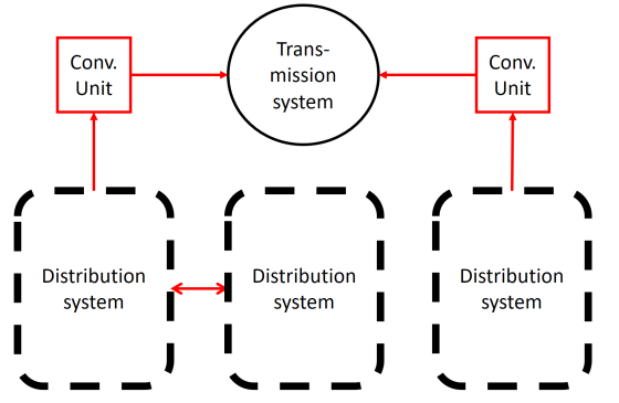
The DK classic instance consists of a representation of the Danish power and district heating system in 2020, see Figure 1. The investment decisions focus on heat production and consist of two CHPs, three heat boilers and three heat pumps: a total of 8 investments.
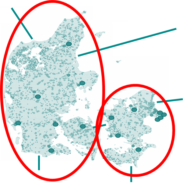
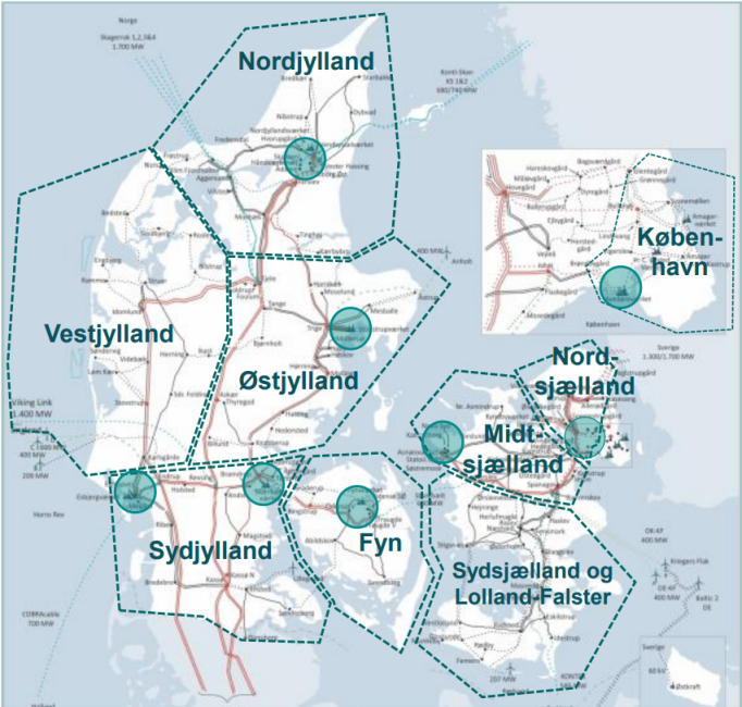
The DK detailed instance consists of the Danish power and district heating system in 2050, see Figure 2. The number of electricity areas are split into eight areas to represent possible future grid bottlenecks. Also, the production system includes PtX technologies (Power to X technologies), hence fuels are represented in greater detail than in DK classic and include parts of the transportation sector. The investment decisions focus on seven PtX plants, modelled through fourteen condensing power plants, seven heat pumps and one storage: a total of 22 investments.
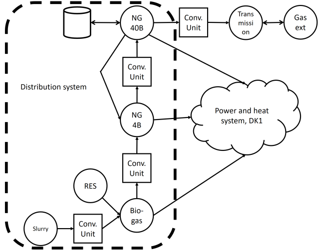
The Gas instance consists of a subpart of the Danish gas transmission and distribution systems in 2020, see Figure 3. The instance introduces large amounts of biogas and investigates investments in two compressors from gas distribution systems to the gas transmission system and one investment in connecting distribution systems directly: a total of 3 investments.
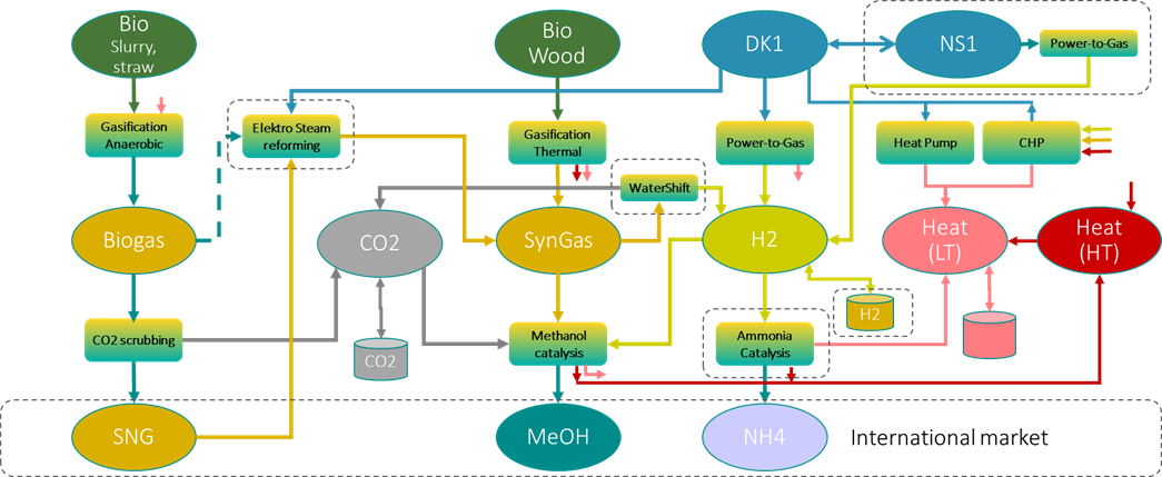
The PtX instance models a Power to X cluster as illustrated in Figure 4. The investment possibilities decide how to dimension the PtX cluster and consists of 19 production units, one heat pump and one interconnection line: a total of 21 investments.
5 Results
The computational evaluation is conducted on a 10 core 2,4 GHz machine with 128 GB RAM, using Gurobi 8.1 as solver. The following abbreviations are used in the remainder of this section: Clustering methods: k for k-means, cc for Cluster Clustering, and lc for Level Correlation clustering. Selection strategies: min for minimum sum, max for maximum sum, median for median sum, and cmean for closest to cluster mean. Finally, we have w for weighted selection, n for non-weighted (fixed weighted) selection, and 28 to represent the 28 generated clusters. Run time results are seen in Table 2 and solution quality gaps in Table 3. Results are analyzed in the following sections.
| DK-classic | DK-detailed | Gas | PtX | |
| Full test instance | 36,45 | 536,06 | 11,71 | 14,69 |
| Dummy Selection | 4,38 | 18,29 | 1,48 | 1,47 |
| k,min,w,28 | 4,21 | 17,42 | 1,34 | 1,54 |
| k,max,w,28 | 5,83 | 22,65 | 1,32 | 1,45 |
| k,median,w,28 | 3,99 | 24,64 | 1,38 | 1,49 |
| k,cmean,w,28 | 4,25 | 15,42 | 1,46 | 1,65 |
| k,random,w,28 | 4,10 | 22,32 | 1,39 | 1,45 |
| cc,min,w,28 | 5,74 | 43,48 | 1,63 | 1,07 |
| cc,max,w,28 | 5,58 | 25,04 | 1,66 | 1,49 |
| cc,median,w,28 | 6,16 | 48,25 | 1,62 | 1,06 |
| cc,cmean,w,28 | 6,04 | 33,26 | 1,67 | 1,51 |
| cc,random,w,28 | 5,66 | 31,73 | 1,71 | 1,21 |
| lc,min,w,28 | 6,21 | 35,76 | 1,54 | 2,15 |
| lc,max,w,28 | 8,20 | 27,42 | 1,93 | 1,53 |
| lc,median,w,28 | 7,01 | 21,86 | 1,90 | 1,68 |
| lc,cmean,w,28 | 6,70 | 35,30 | 1,90 | 1,07 |
| lc,random,w,28 | 7,34 | 34,78 | 1,91 | 1,82 |
| k,min,n,28 | 5,95 | 10,19 | 1,26 | 1,27 |
| k,max,n,28 | 3,89 | 16,82 | 1,25 | 0,88 |
| k,median,n,28 | 5,35 | 16,72 | 1,24 | 0,86 |
| k,cmean,n,28 | 5,72 | 17,40 | 1,25 | 0,86 |
| k,random,n,28 | 4,21 | 15,35 | 1,26 | 1,17 |
| cc,min,n,28 | 6,56 | 21,20 | 1,36 | 1,15 |
| cc,max,n,28 | 6,48 | 19,24 | 1,44 | 1,01 |
| cc,median,n,28 | 5,08 | 18,80 | 1,45 | 0,86 |
| cc,cmean,n,28 | 5,19 | 15,89 | 1,41 | 0,76 |
| cc,random,n,28 | 5,24 | 25,55 | 1,40 | 0,77 |
| lc,min,n,28 | 7,01 | 21,67 | 1,71 | 1,14 |
| lc,max,n,28 | 4,83 | 17,72 | 1,75 | 1,05 |
| lc,median,n,28 | 6,26 | 24,05 | 1,72 | 1,11 |
| lc,cmean,n,28 | 6,41 | 35,26 | 1,74 | 0,93 |
| lc,random,n,28 | 6,54 | 21,10 | 1,74 | 1,00 |
| DK-classic | DK-detailed | Gas | PtX | |
|---|---|---|---|---|
| Dummy Selection | 8% | 5% | 25% | 4% |
| k,min,w,28 | 101% | 3% | 47% | 2% |
| k,max,w,28 | 65% | 18% | 25% | 3% |
| k,median,w,28 | 17% | 4% | 24% | 0% |
| k,cmean,w,28 | 19% | 6% | 39% | 2% |
| k,random,w,28 | 16% | 8% | 40% | 2% |
| cc,min,w,28 | 105% | 4% | 38% | 1% |
| cc,max,w,28 | 30% | 23% | 12% | 7% |
| cc,median,w,28 | 17% | 2% | 37% | 2% |
| cc,cmean,w,28 | 13% | 5% | 35% | 1% |
| cc,random,w,28 | 17% | 5% | 28% | 2% |
| lc,min,w,28 | 23% | 4% | 61% | 1% |
| lc,max,w,28 | 90% | 23% | 17% | 5% |
| lc,median,w,28 | 31% | 6% | 32% | 1% |
| lc,cmean,w,28 | 42% | 9% | 28% | 0% |
| lc,random,w,28 | 6% | 2% | 23% | 0% |
| k,min,n,28 | 102% | 4% | 51% | 1% |
| k,max,n,28 | 66% | 7% | 40% | 6% |
| k,median,n,28 | 9% | 11% | 23% | 1% |
| k,cmean,n,28 | 13% | 4% | 41% | 3% |
| k,random,n,28 | 5% | 2% | 25% | 3% |
| cc,min,n,28 | 75% | 7% | 51% | 2% |
| cc,max,n,28 | 74% | 17% | 49% | 9% |
| cc,median,n,28 | 45% | 2% | 59% | 4% |
| cc,cmean,n,28 | 23% | 3% | 57% | 4% |
| cc,random,n,28 | 37% | 6% | 55% | 8% |
| lc,min,n,28 | 33% | 4% | 68% | 1% |
| lc,max,n,28 | 57% | 20% | 49% | 66% |
| lc,median,n,28 | 40% | 6% | 35% | 2% |
| lc,cmean,n,28 | 47% | 8% | 29% | 2% |
| lc,random,n,28 | 49% | 7% | 33% | 3% |
5.1 Time usage
Time reductions are plotted in Figure 5. Note that the solution times also include pre- and postprocessing of the data instances and not only time for solving the linear program. The time usage savings are consistent across the time aggregation techniques. The average time saving is 90%, which is very satisfying. The time savings are slightly smaller for the DK classic and Gas instances, which could indicate that these instances spend relatively more time on pre- and postprocessing data than the DK detailed and PtX instances.
Generally, the time savings are slightly smaller for the weighted selection algorithms. Recall the weighting from Section 3.3; rounding the number of elements to select from a cluster may increase the total number of selected days. Indeed, the weighted selections result in more than 28 selected days, see Table 4.
| DK classic | DK detailed | Gas | PtX | |
|---|---|---|---|---|
| Dummy selection | 28 | 28 | 28 | 28 |
| k,n,28 | 28 | 28 | 28 | 28 |
| cc,n,28 | 28 | 28 | 28 | 28 |
| lc,n,28 | 28 | 28 | 28 | 28 |
| k,w,28 | 31 | 34 | 34 | 36 |
| cc,w,28 | 37 | 38 | 39 | 39 |
| lc,w,28 | 38 | 37 | 36 | 38 |
5.2 Weighted vs. non-weighted selection
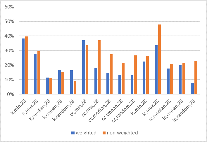
Weighted selection has better performance than non-weighted selection with respect to solution quality in 62% of the time aggregated simulations. The results are illustrated in Figure 6. In 37 of 60 cases, the investment gap decreases with weighted selection. If gaps are averaged across instances, the gap decreases with weighted selection in 11 out of 15 cases. The average of all gaps is 21% for weighted selection and 26% for non-weighted selection. This confirms that weighted selection better represents the full dataset and that outliers are balanced well against the rest of the dataset. The improved quality may partly be due to the increased number of selected days, see Table 4. It is possible to increase the number of selected days for the non-weighted algorithms and compare the results. This would, however, require that the non-weighted algorithms generate more clusters, which again would make comparison more difficult. Instead we continue to compare the algorithms with 28 clusters. The interested reader is referred to Appendix B for results for non-weighted selection with more clusters.
5.3 Selection strategy
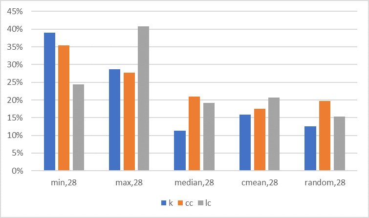
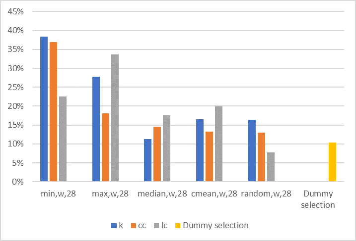
The strategies for selecting elements in each cluster perform differently across the instances. Results averaged across the four instances are illustrated in Figure 7. Clearly, the minimum sum and maximum sum selections have worst performance. Random and median selection vary slightly, while closest to cluster mean gives consistent results. The same pattern is seen, when considering results for weighted selection only, see Figure 8. Selecting only the minimum or maximum sum elements represents the clusters less well. Random performs well which indicates that always selecting the median or closest to cluster mean elements may be too strict.
5.4 New approaches to promote diversification in selected days
Random selection performs well but due to its random nature, results are not consistently good. To eliminate the randomness, we instead seek to mimic differentiated selection.
We propose the MedianMaxMin selection. The approach is only relevant in weighted selection where more than one element may be selected from each cluster. First the median element is selected. If more elements are to be selected from the cluster, the maximum element is selected. Again, if more elements are to be selected, the minimum element is selected. If even more elements are to be selected from the cluster, the selection order repeats.
We also propose the kk-means clustering approach (in short kk). The outer clustering is k-means with squared Euclidean distances where the initial clusters are generated as explained in Section 3.1. The inner clustering is also a k-means with squared Euclidean distances, but this time the initial clusters are formed around the median, maximum sum and minimum sum elements (in the outer cluster).
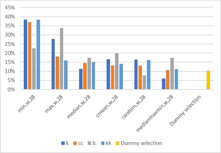
The two approaches are tested. Run times are seen in Table 5 and solution gaps in Table 6. Run times are consistent with the remaining aggregation approaches. Solution gaps are illustrated in Figure 9. MedianMaxMin selection generally performs better than the other selections strategies. Good results are especially achieved together with k-means, cluster clustering and kk-means. Kk-means performs overall well, however, without outperforming the other clustering approaches. It gives consistent results except for min selection, which generally performs poorly regardless of clustering approach.
| DK-classic | DK-detailed | Gas | PtX | |
|---|---|---|---|---|
| k,MedianMaxMin,w,28 | 5,67 | 28,39 | 1,30 | 1,52 |
| cc,MedianMaxMin,w,28 | 5,45 | 21,55 | 1,65 | 2,26 |
| lc,MedianMaxMin,w,28 | 5,27 | 27,24 | 1,57 | 1,28 |
| kk,min,w,28 | 3,86 | 23,35 | 1,48 | 1,20 |
| kk,max,w,28 | 7,35 | 21,78 | 1,48 | 1,36 |
| kk,median,w,28 | 5,56 | 13,88 | 1,50 | 1,45 |
| kk,cmean,w,28 | 5,56 | 26,14 | 1,61 | 1,70 |
| kk,random,w,28 | 4,07 | 24,19 | 1,54 | 1,26 |
| kk,MedianMaxMin,w,28 | 6,33 | 23,10 | 1,51 | 1,35 |
| DK-classic | DK-detailed | Gas | PtX | |
|---|---|---|---|---|
| k,medianmaxmin,w,28 | 4% | 4% | 15% | 1% |
| cc,medianmaxmin,w,28 | 16% | 2% | 21% | 2% |
| lc,medianmaxmin,w,28 | 29% | 7% | 31% | 1% |
| kk,min,w,28 | 104% | 3% | 43% | 3% |
| kk,max,w,28 | 41% | 6% | 7% | 9% |
| kk,median,w,28 | 29% | 9% | 20% | 2% |
| kk,cmean,w,28 | 14% | 2% | 37% | 3% |
| kk,random,w,28 | 12% | 2% | 48% | 3% |
| kk,medianmaxmin,w,28 | 7% | 9% | 23% | 6% |
6 Further analysis
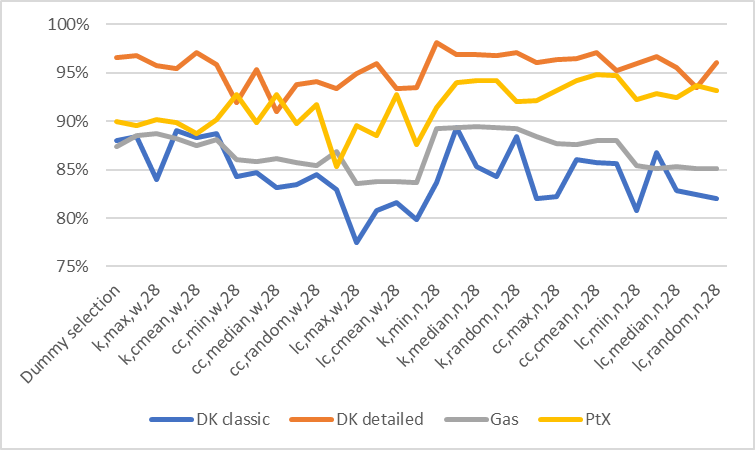
The results reveal different quality across time aggregation techniques and data instance. The data instances are analyzed to better understand the results; specifically, we analyze the behavior of the investments in the optimal solution for the full test instances and what this means to the clustering approaches. Average gaps for the instances are seen in Figure 10.
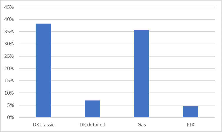
DK-classic: The investments are mainly utilized in the winter period. They are driven by district heating demand. Data in the instance, however, also contains many other fluctuating timeseries, especially connected to the electricity system: demand, RES production, electricity prices in neighboring countries and capacity restrictions on interconnection lines. The clustering methods end up generating clusters and selecting days, which are not relevant to the investments.
Gas: The investments are utilized in the summer period, where demand is low. In these hours, excessive biogas is either moved between distribution systems or sold to the transmission system. Gas demand is, however, not the only varying data in the instance. Electricity prices (considered by gas-fueled CHPs) vary throughout the year. Line pack is modelled as storage space with highest value in the spring. Gas demand varies more outside the summer period (the higher demand, the higher absolute variation). Hence the clustering approaches end up generating clusters and selecting days from other seasons than the summer and the solution quality suffers.
DK-detailed: The investments follow RES production and electricity demand. Most timeseries in the dataset are related to RES production and electricity, which explains the good solution quality.
PtX: The fluctuation of the timeseries correspond well to the entire production system, including the optimal investments. All time aggregation methods thus have good performance.
6.1 Overall best aggregation method
Given the analysis in this section and the results in the previous, we investigate which aggregation method show most promising results.
Dummy selection performs well but the method is not robust towards investments, which are utilized in only part(s) of the simulated year. This is the case for the Gas instance where Dummy Selection ends up with a 25% gap. For this reason, it may not generally be the best approach. It, however, benefits from being very simple to implement and to understand from the analyst’s point of view.
For the clustering approaches, we have already concluded that best performance is achieve with weighted selection and with other selection methods than min and max. The overall best performing method in our survey is k-means clustering with weighted selection and with the MedianMinMax selection strategy. The k-means is simple to implement and the MedianMinMax strategy diversifies selection without introducing the uncertainty of randomness.
We recommend this method but are also aware that this is a close call. This could indicate that the performance bottleneck no longer lies in the clustering or selection itself. This is investigated in the next section on future work.
6.2 Future Work
The clustering methods suffer from generating clusters based on data fluctuations irrelevant to the investment decision. We have identified three ideas to further dive into this.
Future work could focus on methods to better represent data. One method could be to normalize data to take on values between e.g. -1 and 1. This could lead to a fairer comparison of data stemming from different sources, e.g. comparing capacities with prices. This would, however, also erase the absolute amounts and thus treat e.g. large demands equally to small demands. Fluctuations in small timeseries may cause unimportant days to be selected and thus negatively affect the clustering approach.
Future work could also focus on dimensionality reduction, e.g. by considering the subset of data needed to represent the statistical behavior of each day, or by considering the subset of data which correlates with the investment decisions.
Finally, future work could focus on testing the methods on instances with more investment decisions, especially where the utilization of the investment decisions is not correlated. This could possibly better test the difference between the clustering methods, especially if level correlation clustering performs differently than the other three clustering methods.
7 Conclusion
In this paper, we have investigated the performance of clustering techniques across very different energy systems to give a recommendation of a method with overall good performance. We have applied a number of clustering techniques to real-life capacity expansion problems. The clustering techniques all select a subset of days from the datasets, which cover a full year. The applied methods are k-means, hierarchical clustering and a double clustering procedure applying a fuzzy clustering, followed by a hierarchical clustering considering element correlations. Also, we proposed a new method consisting of double k-means clustering.
The methods cluster days and then selects a number of days from each cluster. We have tested several selection strategies from the literature: min, max, median, closest to cluster mean and random. We have also proposed a new selection strategy, MedianMaxMin, which selects elements in the named order. Finally, we have investigated the effect of selecting a single element from each cluster or a weighted number of elements from each cluster.
All in all, this resulted in a comparison of 41 aggregation techniques, and the results were benchmarked against the full datasets. The comparison is evaluated on how well the investment decisions are matched. The methods were tested on four very different energy systems to investigate performance consistency and to analyze if certain energy system aspects are more difficult to replicate through aggregation.
The tests showed that all aggregation techniques resulted in significant time reductions between 78% and 97%. The tests also revealed that weighted selection outperformed selecting exactly one element from each cluster. To the best of our knowledge, this has not been analyzed or concluded previously in the literature. Selecting minimum or maximum elements from each cluster was generally not a good strategy. The new selection method, MedianMaxMin, and clustering method, kk, both performed consistently well. Especially k-means with MedianMaxMin selection showed very good performance, and this is also the clustering approach we recommend.
We also tested Dummy Selection, which simply selects every 13th day. It overall performed surprisingly well. Considering its simplicity, it could be a good alternative to the more complex clustering methods as it is easy to implement and understand.
Future work could focus on how data is considered when clustering. In this paper, all timeseries are considered. A closer analysis of the test instances revealed that this may not be the best approach as data irrelevant to the investments caused the aggregation techniques to select days, which were also irrelevant to the investment decisions.
References
- [1] A. Almaimouni, A. Ademola-Idowu, J. Kutz, A. Negash and D. Kirschen, ”Selecting and Evaluating Representative Days for Generation Expansion Planning”. 2018 Power Systems Computation Conference (PSCC), 2018. doi: 10.23919/PSCC.2018.8442580.
- [2] R. Anand, D. Aggarwal and V. Chahar, ”A Comparative Analysis of Optimization Solvers”. Journal of Statistics and Management Systems 20, 2017. doi: 10.1080/09720510.2017.1395182.
- [3] O. M. Babatunde, J. L. Munda and Y. Hamam, ”A comprehensive state-of-the-art survey on power generation expansion planning with intermittent renewable energy source and energy storage”. International Journal of Energy Research, 2019. doi: 10.1002/er.4388.
- [4] C. Baldwin, K. Dale, and R. Dittrich, ”A Study of the Economic Shutdown of Generating Units in Daily Dispatch”. Power Apparatus and Systems, Part III, Transactions of the American Institute of Electrical Engineers 78, pp. 1272-1282, 1960. doi: 10.1109/AIEEPAS.1959.4500539.
- [5] ”Balmorel”, [Online]. Available: http://www.balmorel.com/.
- [6] C. Batlle and P. Rodilla, ”An Enhanced Screening Curves Method for Considering Thermal Cycling Operation Costs in Generation Expansion Planning”. IEEE Transactions on Power Systems 28, pp. 3683-3691, 2013. doi: 10.1109/TPWRS.2013.2249540
- [7] P. Bendotti, P. Fouilhoux and C. Rottner, ”On the complexity of the Unit Commitment Problem,” Annals of Operations Research, vol. 274, no. 3, pp. 119-130, 2019. doi: 10.1007/s10479-018-2827-x
- [8] T. Brown, D. Schlachtberger, A. Kies, S. Schramm and M. Greiner, ”Synergies of sector coupling and transmission extension in a cost-optimised, highly renewable European energy system.” Energy 160, 2018. doi: 10.1016/j.energy.2018.06.222.
- [9] S. Buchholz, M. Gamst and D. Pisinger, ”A Comparative Study of Aggregation Techniques in relation to Capacity Expansion Energy System Modeling,” TOP 2019, vol. 27, no. 3, pp. 353-405, 2019. doi: 10.1007/s11750-019-00519-z
- [10] M. Carrion and J. Arroyo, ”A Computationally Efficient Mixed-Integer Linear Formulation for the Thermal Unit Commitment Problem”. IEEE Transactions on Power Systems, 21, pp. 1371-1378, 2006. doi: 10.1109/TPWRS.2006.876672.
- [11] A. Dagoumas and N. Koltsaklis, ”Review of models for integrating renewable energy in the generation expansion planning”. Applied Energy 242, pp. 1573-1587, 2019. doi: 10.1016/j.apenergy.2019.03.194.
- [12] J. P. Deane, A. Chiodi, M. Gargiulo and B. O’Gallachoir, ”Soft-linking of a power systems model to an energy systems model”. Energy 42, pp. 303-312, 2012. doi: 10.1016/j.energy.2012.03.052
- [13] J. C. Dunn, ”A Fuzzy Relative of the ISODATA Process and Its Use in Detecting Compact Well-Separated Clusters”. Journal of Cybernetics, 3, pp. 32–57, 1973. doi:10.1080/01969727308546046.
- [14] M. ElNozah, M. Salama and R. Seethapathy, ”A probabilistic load modelling approach using clustering algorithms,” IEEE Power and Energy Society General Meeting, pp. 1-5, 2016. doi: 10.1109/PESMG.2013.6672073
- [15] W. Fisher, ”On Grouping for Maximum Homogeneity”, Journal of The American Statistical Association 53, pp. 789-798, 1958. doi: 10.1080/01621459.1958.10501479.
- [16] A. Flores-Quiroz, R. Palma-Behnke, G. Zakeri and R Moreno, ”A column generation approach for solving generation expansion planning problems with high renewable energy penetration”. Electric Power Systems Research 136, pp. 232-241, 2016. doi: 10.1016/j.epsr.2016.02.011
- [17] M. Fripp, ”Switch: A Planning Tool for Power Systems with Large Shares of Intermittent Renewable Energy”. Environmental Science & Technology 46, pp. 6371–6378, 2012, doi: 10.1021/es204645c.
- [18] R. Green, I. Staffell and N. Vasilakos, ”Divide and Conquer? K-means Clustering of Demand Data Allows Rapid and Accurate Simulations of the British Electricity System,” IEEE Transactions on engineerring management, vol. 61, no. 2, pp. 251-260, 2014. doi: 10.1109/TEM.2013.2284386
- [19] J. Han, M. Kamper and J. Pei, ”10 – Cluster Analysis: Basic Concepts and Methods,” in Data Mining (Third Edition), Morgan Kaufmann, 2012, pp. 443 - 495.
- [20] C. Heuberger, I. Staffell, N. Shah, and N. MacDowell, ”A systems approach to quantifying the value of power generation and energy storage technologies in future electricity networks”. Computers & Chemical Engineering, 2017. doi: 10.1016/j.compchemeng.2017.05.012.
- [21] B. Hua, R. Baldick and J. Wang, ”Representing Operational Flexibility in Generation Expansion Planning Through Convex Relaxation of Unit Commitment”. IEEE Transactions on Power Systems 33, pp. 2272-2281, 2017. doi: 10.1109/TPWRS.2017.2735026.
- [22] IRENA (2017), ”Planning for the Renewable Future: Long-term modelling and tools to expand variable renewable power in emerging economies,” International Renewable Energy Agency, Abu Dhabit, 2017.
- [23] C. Jonghe, E. Delarue, R. Belmans and W. D’haeseleer, ”Determining optimal electricity technology mix with high level of wind power penetration”, Applied Energy 88, pp. 2231-2238, 2011. doi: 10.1016/j.apenergy.2010.12.046
- [24] N. Koltsaklis and A. Dagoumas, ”State-of-the-art generation expansion planning: A review”. Applied Energy 230, pp. 563-589, 2018. doi: 10.1016/j.apenergy.2018.08.087.
- [25] N. Koltsaklis and M. Georgiadis, ”A multi-period, multi-regional generation expansion planning model incorporating unit commitment constraints”. Applied Energy 158, pp. 310-331, 2015. doi:10.1016/j.apenergy.2015.08.054.
- [26] L. Kotzur, P. Markewitz, M. Robinius and D. Stolten, ”Impact of different time series aggregation methods on optimal energy system design”. Renewable Energy 117, 2017. doi: 10.1016/j.renene.2017.10.017
- [27] L. Kotzur, P. Markewitz, M. Robinius, and D. Stolten, ”Time series aggregation for energy system design: Modeling seasonal storage”, Applied Energy 213, 2018. doi: 10.1016/j.apenergy.2018.01.023.
- [28] Y. Liu, R. Sioshansi and A. J. Conejo, ”Hierarchical clustering to find representative operating periods for capacity-expansion modeling,” IEEE Transactions on Power Systems, vol. 33, no. 3, pp. 3029-3039, 2017.
- [29] R. Loulou, U. Remne, A. Kanudia, A. Lehtila and G. Goldstein, ”Documentation for the MARKAL Family of Models – PART 1,” [Online]. Available: http://iea-etsap.org/docs/TIMESDoc-Intro.pdf.
- [30] J. B. MacQueen, ”Some Methods for classification and Analysis of Multivariate Observations”. Proceedings of 5th Berkeley Symposium on Mathematical Statistics and Probability 1, pp. 281–297, 1967.
- [31] R. Mallipeddi and P. Suganthan, ”Unit commitment - A survey and comparison of conventional and nature inspired algorithms”. Int. J. of Bio-Inspired Computation 6, pp. 71-90, 2014. doi: 10.1504/IJBIC.2014.060609.
- [32] J. H. Merrick, ”On representation of temporal variability in electricity capacity planning models”, Energy Economics 59, pp. 261-274, 2016. doi: 10.1016/j.eneco.2016.08.001.
- [33] P. Nahmmacher, E. Schmid, L. Hirth and B. Knopf, ”Carpe Diem: A Novel Approach to Select Representative Days for Long-Term Power System Models with High Shares of Renewable Energy Sources,” Energy, vol. 112, pp. 430-442, 2016. doi: 10.1016/j.energy.2016.06.081.
- [34] A. Nogales, S. Wogrin and E. Centeno, ”The impact of technical operational details on generation expansion in oligopolistic power markets”. IET Generation Transmission & Distribution 10, 2016. doi: 10.1049/iet-gtd.2015.1148.
- [35] M. Nicolos, A. Mills and R. Wiser, ”The importance of high temporal resolution in modeling renewable energy penetration scenarios,” 9th Conference on Applied Infrastructure Research, 2011.
- [36] V. Oree, S. Z. Sayed Hassen and P. Fleming, ”Generation expansion planning optimisation with renewable energy integration: A review.” Renewable and Sustainable Energy Reviews 69, pp. 790-803, 2017. doi: 10.1016/j.rser.2016.11.120.
- [37] J. Ostrowski, M. Anjos, and A. Vannelli, ”Tight Mixed Integer Linear Programming Formulations for the Unit Commitment Problem”. IEEE Transactions on Power Systems 27, pp. 39-46, 2012. doi: 10.1109/TPWRS.2011.2162008.
- [38] B. Palmintier and M. Webster, ”Impact of Operational Flexibility on Electricity Generation Planning With Renewable and Carbon Targets”. IEEE Transactions on Sustainable Energy, 2015. doi: 10.1109/TSTE.2015.2498640
- [39] K. Poncelet, E. Delarue, D. Six, J. Dueinck and W. D’haeseleer, ”Impact of the level of temporal and operational detail in energy-system planning models.,” Applied Energy, vol. 162, no. 58, pp. 631-643, 2016. doi: 10.1016/j.apenergy.2015.10.100.
- [40] K. Poncelet, H. Hoschle, E. Delarue, A. Virag and W. D’haeseleer, ”Selecting representative days for capturing the implications of integrating intermittent renewables in generation expansion problems”. IEEE Transactions on Power Systems, 2016. doi: 10.1109/TPWRS.2016.2596803.
- [41] K. Poncelet, E. Delarue, and W. D’haeseleer, ”Unit commitment constraints in long-term planning models: Relevance, pitfalls and the role of assumptions on flexibility”. Applied Energy 258, 113843, 2019. doi: 10.1016/j.apenergy.2019.113843.
- [42] H. K. Ringkjøb, P. Haugan, and I. Solbrekke, ”A review of modelling tools for energy and electricity systems with large shares of variable renewables”. Renewable and Sustainable Energy Reviews 96, pp. 440-459, 2018. doi: 10.1016/j.rser.2018.08.002.
- [43] D. F. Rogers, R. D. Plante, R. T. Wong and J. R. Evans, ”Aggregation and disaggregation Techniques and Methodology in Optimization,” Operations Research, vol. 39, no. 4, pp. 553-582, 1991. doi: 10.1287/opre.39.4.553
- [44] H. Sadeghi and A. Abdollahi, ”A comprehensive sequential review study through the generation expansion planning”. Renewable and Sustainable Energy Reviews 67, pp. 1672-1682, 2017. doi: 10.1016/j.rser.2016.09.046.
- [45] A. Schwele and J. Kazempour and P. Pinson, ”Do unit commitment constraints affect generation expansion planning? A scalable stochastic model”. Energy Systems 2018. doi: 10.1007/s12667-018-00321-z
- [46] I. Scott, P. Carvalho and A. Botterud and C. Silva, ”Clustering representative days for power systems generation expansion planning: Capturing the effects of variable renewables and energy storage”, Applied Energy 253, 113603, 2019. doi: 10.1016/j.apenergy.2019.113603.
- [47] A. Shortt, J. Kiviluoma and M. O’Malley, ”Accommodating Variability in Generation Planning”. IEEE Transactions on Power Systems 28, pp. 158-169, 2013. doi: 10.1109/TPWRS.2012.2202925
- [48] ”Sifre – Simulation of Flexible and Renewable Energy Systems,” [Online]. Available: https://energinet.dk/-/media/0C7AA9C78EBE428580CAB85E120129CB.pdf.
- [49] F. J. de Sisternes, M. D. Webster and I. J. Pérez-Arriaga, ”The Impact of Bidding Rules on Electricity Markets With Intermittent Renewables”. IEEE Transactions on Power Systems 30, pp. 1603-1613, 2015. doi: 10.1109/TPWRS.2014.2355775.
- [50] H. Teichgraeber and A. R. Brandt, ”Clustering methods to find representative periods for the optimization of energy systems : An initial framework and comparison,” Applied Energy, vol. 239, pp. 1283-1293, 2019. doi: 10.1016/j.apenergy.2019.02.012
- [51] A. Viana and J. P. Pedroso, ”A new MILP-based approach for unit commitment in power production planning”. International Journal of Electrical Power & Energy Systems Volume 44 (1), pp. 997-1005, 2013. doi: 10.1016/j.ijepes.2012.08.046
- [52] M. Welsch, P. Deane, M. Howells, B. O’Gallachóir, F. Rogan, M. Bazilian and H. Rogner, ”Incorporating flexibility requirements into long-term energy system models – A case study on high levels of renewable electricity penetration in Ireland”. Applied Energy 135, pp. 600-615, 2014. doi: 10.1016/j.apenergy.2014.08.072.
- [53] S. Xie, Z. Hu, and J. Wang, ”Scenario-based comprehensive expansion planning model for a coupled transportation and active distribution system.” Applied Energy 255, 2019. doi: 10.1016/j.apenergy.2019.113782.
Appendix A Capacity Expansion Modelling in Sifre
This Appendix explains how capacity expansion is added to the energy system model formulation in Sifre [48]. The notation is kept at a high level, such that the reader can understand the formulations without reading the extensive nomenclature in [48]. The set T defines the time steps, and index i is used to denote the relevant component. Also, z denotes the objective function for the energy system model formulation in [48].
Storage
The variable decides the invested inventory level of storage
. The formulation adds the investment costs to the objective. The
constraints ensure that the invested amount satisfies the specified
lower and upper bound, and that the storage inventory level never
exceeds the invested inventory level.
| (18) | |||||
| s. t. | (19) | ||||
| (20) | |||||
Interconnection line
The variable decides the invested capacity of the
interconnection line . The formulation adds the investment costs to
the objective function. The constraints ensure that the invested
amount satisfies the specified lower and upper bound, and that the
flow on the interconnection line never exceeds the invested capacity.
| (21) | |||||
| s. t. | (22) | ||||
| (23) | |||||
Renewable units
The variable decides the invested capacity of the renewable unit
. The formulation adds the investment costs to the objective
function. The constraints ensure that the invested amount satisfies
the specified lower and upper bound, and that the renewable production
never exceeds the invested capacity. The parameter
defines the possible RES production subject to e.g. available wind or
solar. If curtailment is allowed, production in an hour does not have
to equal the available RES production.
| (24) | |||||
| s. t. | (25) | ||||
| if curtailment is allowed: | |||||
| (26) | |||||
| if curtailment is not allowed: | |||||
| (27) | |||||
Condensation plants, heat boilers, heat pumps, electric boilers and backpressure CHPs
The following formulation is valid for production units, which either
only produces one type of energy, or where the relationship between
the primary and second energy production is fixed (e.g. power and heat
production in backpressure units). In the latter case, the investment
bounds are specified according to the primary production. The
variable decides the invested capacity of the production
unit . The formulation in the following adds the investment costs to
the objective function. The constraints ensure that the invested
amount satisfies the specified lower and upper bound, and that the
production of the unit never exceeds the invested capacity.
| (28) | |||||
| s. t. | (29) | ||||
| (30) | |||||
Extraction CHPs
The following formulation is valid for extraction production
units. The relationship between the primary and secondary energy
production (power and heat) is defined by a PQ diagram, see Figure 11.
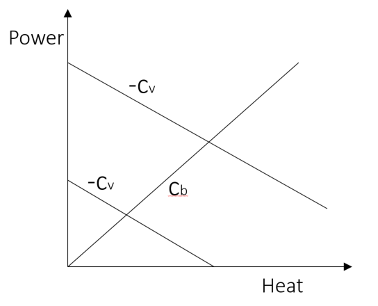
The variable decides the invested capacity of the production unit . The formulation in the following adds the investment costs to the objective function. The constraints ensure that the invested amount satisfies the specified lower and upper bound, and that the production of the unit never exceeds the invested capacity. Both the primary and secondary production must be considered to ensure the correct capacity for the extraction unit.
| (31) | |||||
| s. t. | (32) | ||||
| (33) | |||||
where defines the upper bound relationship between heat and power production in the PQ diagram, see Figure 11.
Appendix B Results for non-weighted selection with more clusters
Weighted selection algorithms end up selecting more elements than non-weighted, see Section 3.3. The same number of selected elements can be achieved by allowing the algorithms with non-weighted selection to generate more clusters. For example, if an algorithm with weighted selection ends up selecting 32 days, then we can configure the algorithm with non-weighted selection to generate 32 clusters. As the latter selects one element from each cluster, it ends up selecting 32 days. The double clustering approaches sets the number of outer clusters to the total number of desired clusters divided by 4. In case of a total of 32 clusters, the approaches generate 8 outer clusters. In case of a total of 29 clusters, the approaches generate 7 outer clusters. Each outer cluster is re-clustered into four inner clusters. For this reason, the final number of clusters may variate slightly from the desired amount for the double clustering approaches. Furthermore, the total number of selected elements may also vary slightly for the cc and kk approaches because the outer K means algorithm may generate clusters with few elements, e.g. 1 element, and the inner clustering approaches can thus not generate “enough” clusters.
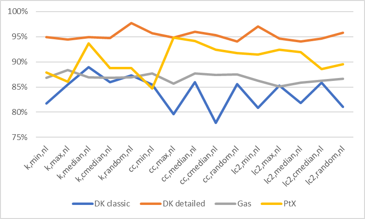
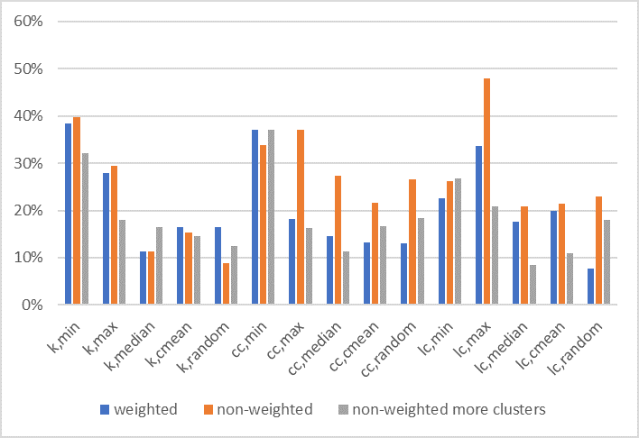
Time savings are consistent with previous results, see Table 7 and Figure 12. Quality results can be seen in Table 8 and Figure 13. The results reveal that weighted selection is best in 41% of the tests, non-weighted in 21% and non-weighted with more clusters in 38% of the instances. Overall, weighted selection still has best performance with respect to quality, though generating more clusters is also a very reasonable approach.
| DK-classic | DK-detailed | Gas | PtX | |
|---|---|---|---|---|
| k,min,nl | 6,65 | 27,13 | 1,54 | 1,78 |
| k,max,nl | 5,28 | 29,68 | 1,36 | 2,05 |
| k,median,nl | 4,02 | 27,39 | 1,53 | 0,93 |
| k,cmedian,nl | 5,12 | 28,41 | 1,54 | 1,65 |
| k,random,nl | 4,61 | 12,27 | 1,53 | 1,65 |
| cc,min,nl | 5,3 | 23,22 | 1,44 | 2,24 |
| cc,max,nl | 7,44 | 27,72 | 1,68 | 0,76 |
| cc,median,nl | 5,12 | 21,79 | 1,44 | 0,86 |
| cc,cmedian,nl | 8,06 | 25,25 | 1,47 | 1,11 |
| cc,random,nl | 5,25 | 32,05 | 1,46 | 1,21 |
| lc2,min,nl | 6,97 | 15,98 | 1,61 | 1,25 |
| lc2,max,nl | 5,36 | 28,64 | 1,75 | 1,12 |
| lc2,median,nl | 6,62 | 31,73 | 1,65 | 1,18 |
| lc2,cmedian,nl | 5,15 | 28,98 | 1,61 | 1,68 |
| lc2,random,nl | 6,89 | 22,34 | 1,57 | 1,54 |
| DK-classic | DK-detailed | Gas | PtX | |
|---|---|---|---|---|
| k,min,nl | 101% | 5% | 23% | 1% |
| k,max,nl | 41% | 10% | 16% | 4% |
| k,median,nl | 41% | 2% | 20% | 3% |
| k,cmedian,nl | 15% | 4% | 37% | 2% |
| k,random,nl | 20% | 3% | 24% | 2% |
| cc,min,nl | 106% | 5% | 35% | 3% |
| cc,max,nl | 22% | 8% | 25% | 10% |
| cc,median,nl | 9% | 2% | 29% | 5% |
| cc,cmedian,nl | 19% | 3% | 40% | 4% |
| cc,random,nl | 33% | 7% | 28% | 5% |
| lc2,min,nl | 64% | 3% | 40% | 0% |
| lc2,max,nl | 38% | 15% | 23% | 7% |
| lc2,median,nl | 23% | 2% | 7% | 1% |
| lc2,cmedian,nl | 19% | 4% | 21% | 1% |
| lc2,random,nl | 27% | 3% | 41% | 1% |
