Quantum refrigerators in finite-time cycle duration

Abstract

We derive cooling rate and coefficient of performance as well as their variances for a quantum Otto engine proceeding in finite-time cycle period. This machine consists of two driven strokes, where the system isolated from the heat reservoir undergoes finite-time unitary transformation, and two isochoric steps, where the finite-time system-bath interaction durations take the system away from the equilibrium even at the ends of the two stages. We explicitly calculate the statistics of cooling rate and coefficient of performance for the machine operating with an analytically solvable two-level system. We clarify the role of finite-time durations of four processes on the machine performance. We show that there is the trade-off between the performance parameter and its corresponding variance, thereby indicating that the cooling rate or coefficient of performance can be enhanced, but at the cost of increasing the corresponding fluctuations.

PACS number(s): 05.70.Ln

I Introduction

A refrigerator as an inverse operation of a heat engine transfers energy from a cold thermal bath of temperature $T_{h}$ to a a hot one with temperature $T_{c}$ by consuming work. Quantum refrigerators well as quantum heat engines use quantum systems as their working substance and can be classified either cyclic Aba12 ; Su16 ; Fel00 ; Quan07 ; Ass19 ; Hong20 ; Rez06 or steady-state Kos14 ; Cle12 ; Mas19 ; Ton05 ; Lev12 ; Lin10 models. The quantum Otto cycle of operation, as a typical example of cyclic machines, is controlled by the segments of time that the working system is coupled to a hot and a cold bath, and by the time interval required to driving the control parameter of the system. It was most studied Aba12 ; Su16 ; Fel00 ; Ass19 ; Hong20 ; Rez06 ; Ale15 ; Lee20 as it is easier to analyze and realize. To describe the performance characteristics of a refrigerator, one introduces the coefficient of performance (COP) that is defined as the ratio of heat absorbed from the cold reservoir and work input. An upper bound on the COP imposed by the second law of thermodynamic is given by the Carnot COP: $\varepsilon_{C}=T_{c}/(T_{h}-T_{c})$, which, however, requires infinitesimally slow transitions between thermodynamic states and thus produces vanishing cooling rate. Hence, the refrigerators actually operate far from the infinite long time limit in order for positive cooling rate to be produced Wang12 ; Tom12 ; Hu13 ; Izu15 . The finite cooling rate for a cyclic refrigerator consisting of a sequence of thermodynamic processes indicates that each process must proceed in finite time. For an adequate description of an actual machine, the effects induced by finite-time duration along any thermodynamic stroke on heat and work have to be considered.

While in a macroscopic system the work and heat are deterministic, for a microscopic quantum system (with a limited number of freedoms) these physical variables become random due to non-negligible thermal Sei12 ; Sek10 and quantum Esp09 ; Cam11 fluctuations. Theoretical and experimental investigation on the statistics of work Esp14 ; Quan20 ; Liu19 ; Sol13 ; Hek13 ; Bat14 ; Cer17 and heat Rah12 ; Den18 ; Gas14 has attracted much interest in the literature. On the other hand, for heat engines the statistics of power Hong20 ; Hol18 ; Hol14 ; Wang19 and efficiency Lutz20 ; Vro16 ; Jiang15 ; Vro20 ; Ver14 ; Ver15 ; Par16 has been analyzed, under the assumption that either system-bath interaction interval or unitary driving process is quasistatic. However, a unified thermodynamic description of quantum refrigerators with non-negligible quantum and thermal fluctuations, particularly when every thermodynamic stroke of these machines evolves in finite time, is available.

In the present paper, we study the thermodynamics of a quantum Otto refrigerator where all the four strokes proceed in finite time, within a framework of stochastic thermodynamics. Having determined distribution functions for heat and work, we derive general formulae for the COP and cooling load as well as their variances. With these we then analyze a quantum Otto cycle working with a two-level system which is exactly solvable analytically. We discuss the effects of thermal and quantum fluctuations on finite-time performance and the statistics of the machine, and also demonstrate that there is trade-off of the physical variable (COP or cooling rate) and its fluctuations. We finally show that, the average COP $\langle\varepsilon\rangle$ can be always larger than the conventional thermodynamic COP $\varepsilon_{th}$ for adiabatic driving, but it can be equal to or smaller than COP $\varepsilon_{th}$ for nonadiabatic driving.

II The probability of stochastic COP for quantum otto refrigerators

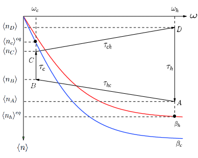
Figure 1: (Color online) Schematic diagram of a quantum Otto refrigeration cycle operating with a two-level system in $(\omega,n)$ plane. The cycle consists of the two adiabatic strokes (connecting states $A$ and $B$, and $C$ and $D$), where the system isolated from the heat reservoir evolves unitary transformation, and two isochoric strokes (connecting states $B$ and $C$, and $D$ and $A$), where the system is kept in thermal contact with the cold and the hot reservoir, respectively. The average population $n_{3}$ ($n_{1}$) at the end of the cold (hot) isochoric stroke would approach its asymptotic value $n_{c}^{eq}$ ($n_{h}^{eq}$), when and only when the system-bath interaction duration $\tau_{c}$ ($\tau_{h}$) tends to be infinitely long.

The quantum Otto cycle under consideration is sketched in Fig. 1. It consists of two isochoric branches, one with a cold and another with a hot heat reservoir where the Hamiltonian is kept constant, and two other strokes, where the system undergoes unitary transformation while isolating from the thermal reservoirs. In the adiabatic branch $A\rightarrow B$, the system is isolated from any heat reservoir and undergoes a unitary expansion from time $t=0$ to $t=\tau_{hc}$. Initially, the system is assumed to be with local thermal equilibrium at inverse temperature $\beta_{A}(\geq\beta_{h})$. The probability distribution of stochastic work done by the system, $w_{hc}$, can be given by Tal07

$$p(w_{hc})=\sum_{n,m}\delta[w_{hc}-(E_{m}^{c}-E_{n}^{h})]p_{n\rightarrow m}^{\tau_{hc}}p_{n}^{0}(\beta_{A}).$$ (1)

where $E_{n}^{h}$ and $E_{m}^{c}$ are the respective energy eigenvalues at the initial and final instants along this expansion. Here $p_{n}^{0}(\beta_{A})=\frac{e^{-\beta_{A}E^{h}_{n}}}{Z_{A}}$, with the partition funciton $Z_{A}=\sum_{n}e^{-\beta E_{n}}$, denotes the thermal occupation probability at instant $A$, and $p_{n\rightarrow m}^{\tau_{hc}}=|\langle n|U_{\mathrm{exp}}|m\rangle|^{2}$ is the transition probability from eigenstate $|n\rangle$ and $|m\rangle$, with the unitary time evolution operator $U_{\mathrm{exp}}$. and the population $\langle n\rangle$ remains unchanged in the adiabatic stage ($\xi=0$). If the system Hamiltonian evolves slowly enough wherein the quantum adiabatic condition Born28 is satisfied in time interval $\tau_{hc}$, the the system remains in the same state and the transition probability therefore satisfies $p_{n\rightarrow m}^{\tau_{hc}}=\delta_{nm}$, with the Dirac's delta function $\delta$.

In the next step $B\rightarrow C$, the quantum system with constant frequency $\omega=\omega_{c}$ is kept in contact with a cold thermal bath of inverse temperature $\beta_{c}$ during a period $\tau_{c}$. The probability density of the stochastic heat $q_{c}$ can be determined by conditional distribution to arrive at

$$p(q_{c}|w_{hc})=\sum_{k,l}\delta[q_{c}-(E_{l}^{c}-E_{k}^{c})]p_{k\rightarrow l}^{\tau_{c}}p_{k}^{\tau_{hc}},$$ (2)

where $p_{k}^{\tau_{hc}}$ is the occupation probability at time $t=\tau_{hc}$ and it satisfies the constraint $p_{k}^{\tau_{hc}}=\delta_{km}$. We assume that at the end of the system-bath interaction interval, the system is at the local thermal equilibrium state with inverse temperature $\beta_{C}(\geq\beta_{c}^{r})$, thereby indicating that $p_{k\rightarrow l}^{\tau_{c}}={e^{-\beta_{C}E^{c}_{l}}}/{Z_{C}}$ with partition function $Z_{C}=\sum_{l}{e^{-\beta_{C}E^{c}_{l}}}$. Without loss of generality, the internal energy of system along the isochoric process can be expressed as $\langle n(t)\rangle=[Z(t)]^{-1}\sum_{n}ne^{-\beta(t)E_{n}^{c}},$ where $\langle n\rangle$ is the population (which is also the the expectation value of the particle number operator in Appendix A). When the time duration $\tau_{c}$ tends to be infinity, the mean population $n_{C}$ at end of the isochoric process approaches the equilibrium value,

$$\langle n_{c}\rangle^{eq}\equiv n(\tau_{c}\rightarrow\infty\rangle=Z^{-1}\sum_{n}ne^{-\beta_{c}E_{n}},$$ (3)

with $Z_{c}=\sum_{n}ne^{-\beta_{c}E_{n}}$. It is shown in Appendix A that the dynamics of the system along the thermalization can be described by the motion equation of population, which gives

$$\langle n_{c}\rangle^{eq}=\langle n_{c}\rangle^{eq}+[\langle n_{B}\rangle-\langle n_{c}\rangle^{eq}]e^{-\gamma_{c}\tau_{c}},$$ (4)

where $\langle n_{C}\rangle=\langle n(\tau_{hc}+\tau_{c})\rangle$ and $\langle n_{B}\rangle=\langle n(\tau_{hc})\rangle$, and $\gamma_{c}$ is the thermal conductivity when $\omega=\omega_{c}$.

On the adiabatic compression $C\rightarrow D$, the system is isolated in time duration $\tau_{ch}$ while the energy gap $\omega$ varies from $\omega_{c}$ to $\omega_{h}$. For given work output $w_{hc}$ and the heat $q_{c}$ released from the system, the probability density of stochastic work input is given by

$$p(w_{ch}|q_{c},w_{hc})=\sum\delta[w_{ch}-(E_{j}^{h}-E_{i}^{c})]p_{i\rightarrow j}^{\tau_{ch}}p_{i}^{\tau_{hc}+\tau_{c}},$$ (5)

where the occupation probability $p_{i}^{\tau_{hc}+\tau_{c}}=\delta_{il}$, and $p_{i\rightarrow j}^{\tau_{ch}}=|\langle i|U_{\mathrm{com}}|j\rangle|^{2}$ is transition probability from eigenstate $|i\rangle$ and $|j\rangle$, with the time evolution operator $U_{\mathrm{com}}$ along the compression.

In the fourth step $D\rightarrow A$, the system is coupled to a hot reservoir of inverse temperature $\beta_{h}$ in time duration $\tau_{h}$ while keeping its frequency in a constant with $\omega=\omega_{h}$. Since the system returns to its initial state $A$ after the cycle period $\tau_{cycle}=\tau_{hc}+\tau_{c}+\tau_{ch}+\tau_{h}$, we will do not derive the expression of the stochastic heat exchanged $q_{h}$ along this process. As shown in Appendix A, the populations at the beginning and end of the heating process ($\langle n_{D}\rangle$ and $\langle n_{A}\rangle$) satisfies the constraint:

$$\langle n_{A}\rangle=\langle n_{h}\rangle^{eq}+[\langle n_{D}\rangle-\langle n_{h}\rangle^{eq}]e^{-\gamma_{h}\tau_{h}},$$ (6)

where $\langle n_{A}\rangle=\langle(\tau_{cycle}),\langle n_{D}\langle=\langle n(\tau_{cycle}-\tau_{h})\rangle$,

$$\langle n_{h}\rangle^{eq}\equiv\langle n(\tau_{h}\rightarrow\infty)\rangle^{eq}=Z_{h}^{-1}\sum_{n}ne^{-\beta_{h}E_{n}}$$ (7)

with $Z_{h}=\sum_{n}e^{-\beta_{h}E_{n}}$, and $\gamma_{h}$ is the thermal conductivity between the system and the hot reservoir.

The probability $p(w_{ch},q_{c},w_{hc})$ for the machine which has certain values of $w_{ch},q_{c},w_{hc}$ can be calculated from the the chain rule for condition probabilities $p(w_{ch},q_{c},w_{hc})=p(w_{ch}|q_{c},w_{hc})p(q_{c}\big{|}w_{hc})p(w_{hc})$:

$$\begin{split}p(w_{ch},q_{c},w_{hc})=&\sum\delta\left[q_{c}-\left(E_{k}^{c}-E_{m}^{c}\right)\right]\delta\left[w_{hc}-\left(E_{m}^{c}-E_{n}^{h}\right)\right]\delta\left[w_{ch}-\left(E_{l}^{h}-E_{k}^{c}\right)\right]\\ &\times|\langle n|U_{\mathrm{exp}}|m\rangle|^{2}|\langle i|U_{\mathrm{com}}|j\rangle|^{2}\frac{e^{-\beta_{A}E^{h}_{n}}e^{-\beta_{C}E^{c}_{k}}}{Z_{A}Z_{C}}.\end{split}$$ (8)

In deriving this, we have used Eqs. (1), (2) and (5). For the quantum Otto refrigerator, the stochastic coefficient of performance reads $\varepsilon={q_{c}}/({w_{hc}+w_{ch}})$. It follows, integrating over all values of $w_{ch},q_{c},w_{hc}$, that the probability distribution $p(\varepsilon)$ becomes

$$p\left(\varepsilon\right)=\sum_{m,n,i,j}\delta\left(\epsilon-\frac{E_{k}^{c}-E_{m}^{c}}{E_{m}^{c}-E_{n}^{h}+E_{l}^{h}-E_{k}^{c}}\right)\times\frac{e^{-\beta_{A}E^{h}_{n}}e^{-\beta_{C}E^{c}_{k}}}{Z_{A}Z_{C}}|\langle n|U_{\mathrm{exp}}|m\rangle|^{2}|\langle i|U_{\mathrm{com}}|j\rangle|^{2}.$$ (9)

While for adiabatic driving, the system remains in the same state ($n=m,i=j$), in the nonadiabatic driving the transition probability $|\langle n|U_{\mathrm{exp}}|m\rangle|^{2}$ (or $|\langle i|U_{\mathrm{com}}|j\rangle|^{2})$ is positive due to transitions between sates $n$ and $m$ (or $i$ and $j$). For the quantum Otto refrigerator, its efficiency statistics is fully determined by the unitary time evolution for the adiabatic expansion and compression ($U_{\mathrm{exp}}$ and $U_{\mathrm{com}}$), and by the finite-time system dynamics along the thermalization processes, when the two temperatures of the two heat reservoirs ($\beta_{h}$ and $\beta_{c}$) are given.

III a quantum Otto refrigerator using a two-level system

We now consider a quantum Otto refrigerator operating with a two-level system of the eigenenergies $E_{+}=-\hbar\omega/2$ and $E_{-}=-\hbar\omega/2$. If the unitary expansion and compression during the Otto cycle (from $\omega_{h}$ to $\omega_{c}$ to $\omega_{h}$ and vice versa) is such that there is a probability of level transitions due to quantum fluctuations, then there is a probability that population $\langle n\rangle$ may change with varying time. After a simple calculation (see Appendix B), we find that

$$\langle n_{B}\rangle=(1-2\xi)\langle n_{A}\rangle,~{}\langle n_{D}\rangle=(1-2\xi)\langle n_{C}\rangle$$ (10)

where $\xi=|\langle\pm|U_{\mathrm{exp}}|\mp\rangle|^{2}=|\langle\pm|U_{\mathrm{com}}|\mp\rangle|^{2}$ is called the adiabacity parameter indicating the probability of transition between state $|+\rangle$ and $|-\rangle$ during the compression or expansion. As shown in Fig. 1, the populations at any instant along the cycle is negative, which means that $\xi$ must be situated between $0\leq\xi<1/2$. The probability of no state transition along either driving phase is accordingly $|\langle\pm|U_{\mathrm{exp}}|\pm\rangle|^{2}=|\langle\pm|U_{\mathrm{com}}|\pm\rangle|^{2}=1-\xi$. The adiabaticity parameter $\xi$ depends on the the speed at which the driving process is performed Aba12 ; Ass19 ; Lutz20 . When the time scale of the state change is much larger than that of the dynamical one, the quantum adiabatic condition is satisfied and the population $\langle n\rangle$ remains unchanged in the adiabatic stage ($\xi=0$). Rapid change in the control field $\omega$, however, leads to nonadiabatic behavior ($\xi>0$) which can understood as inner friction Rez06 ; Fel00 ; Ale15 ; Cor15 ; Cam19 ; Pla14 causing state transitions. Equation (10) shows that $\langle n_{C}\rangle>\langle n_{B}\rangle$ and $\langle n_{D}\rangle>\langle n_{C}\rangle$ for $\xi>0$ (see also Fig. 1), as lies in the fact that the finite time duration of the expansion and compression accounts for the nonadiabatic inner friction related to the irreversible entropy production.

Using Eqs. (4), (6), and (10), it follows that the populations $\langle n_{A}\rangle$ and $\langle n_{C}\rangle$ can be expressed in terms of the equilibrium populations $\langle n_{h}\rangle^{eq}$ and $\langle n_{c}\rangle^{eq}$,

$$\langle n_{A}\rangle=\langle n_{h}\rangle^{eq}+\Delta_{h},\langle n_{C}\rangle=\langle n_{c}\rangle^{eq}+\Delta_{c}$$ (11)

where

$$\Delta_{h}=\frac{\left(2\xi-1\right)\left[\left(2\xi-1\right)\langle n_{h}\rangle+\langle n_{c}\rangle^{eq}\right]-y\left[\langle n_{h}\rangle+\left(2\xi-1\right)\langle n_{c}\rangle^{eq}\right]}{xy-\left(2\xi-1\right)^{2}},$$ (12)

$$\Delta_{c}=\frac{\left(2\xi-1\right)\left[\left(2\xi-1\right)\langle n_{c}\rangle+\langle n_{h}\rangle^{eq}\right]-x\left[\langle n_{c}\rangle+\left(2\xi-1\right)\langle n_{h}\rangle^{eq}\right]}{xy-\left(2\xi-1\right)^{2}},$$ (13)

with $x=e^{\gamma_{h}\tau_{h}}$ and $y=e^{\gamma_{c}\tau_{c}}$. Hereafter we will refer $x$ and $y$ rather than $\tau_{h}$ and $\tau_{c}$ as the time durations along the hot and cold isochoric branches for simplicity. Here $\langle n_{c}\rangle^{eq}$ defined in Eq. (3) and $\langle n_{h}\rangle^{eq}$ in Eq. (7) can be obtained using the same approach as that described in Appendix A for the derivation of Eq. (B.2) to arrive at ($\hbar\equiv 2$)

$$\langle n_{c}\rangle^{eq}=-\frac{1}{2}\tanh(\beta_{c}\omega_{c}),\langle n_{h}\rangle^{eq}=-\frac{1}{2}\tanh(\beta_{h}\omega_{h}),$$ (14)

which is achieved in quasi-static limit ($x,y\rightarrow\infty$) when $\Delta_{c,h}\rightarrow 0$. While for the finite-time system-bath interaction interval the system is away from the thermal equilibrium, the populations $\langle n_{C}\rangle$ and $\langle n_{A}\rangle$ approach the thermal values $\langle n_{c}\rangle^{eq}$ and $\langle n_{h}\rangle^{eq}$, respectively, when these intervals go to the infinite long time limit. Therefore, $\Delta_{c}$ and $\Delta_{h}$ indicate how far the two isochoric processes deviates from the quasistatic limit.

From Eqs. (1) and (2), the average heat injection, $\langle q_{c}\rangle=\int\int q_{c}p(q_{c}|w_{hc})p(w_{hc})dw_{hc}dq_{c}$ can be obtained as $(\hbar\equiv 2)$

$$\langle q_{c}\rangle=2\omega_{c}\left[\langle n_{c}\rangle+\Delta_{c}+\left(2\xi-1\right)\left(\langle n_{h}\rangle+\Delta_{h}\right)\right],$$ (15)

Integrals over the distribution function $p\left(q_{c}|w_{hc}\right)p\left(w_{hc}\right)$ yield the second moments of absorbed heat $q_{c}$, $\langle q_{c}^{2}\rangle=\int\int q_{c}^{2}\left(w_{hc}\right)p\left(q_{c}|w_{hc}\right)dw_{hc}dq_{c}$, which reads $\langle q_{c}^{2}\rangle=8\omega_{c}^{2}\left[{1}/{4}+\left(2\xi-1\right)\left(\langle n_{h}\rangle+\Delta_{h}\right)\left(\langle n_{c}\rangle+\Delta_{c}\right)\right].$ The variance of absorbed heat $q_{c}$, $\delta q_{c}^{2}=\langle q_{c}^{2}\rangle-\langle q_{c}\rangle^{2}$, then becomes

$$\delta{q_{c}^{2}}=4\omega_{c}^{2}\left[\frac{1}{2}-\left(2\xi-1\right)^{2}\left(\langle n_{h}\rangle+\Delta_{h}\right)^{2}-\left(\langle n_{c}\rangle+\Delta_{c}\right)^{2}\right].$$ (16)

These variances are upper limited by the value of $2\omega_{c}^{2}$ and they become $\delta{q_{c}^{2}}=4\omega_{c}^{2}\left[\frac{1}{2}-\langle(n_{h}\rangle)^{2}-\left(\langle n_{c}\rangle^{eq}\right)^{2}\right]$ for the quasistatic cycle.

As $\langle\dot{q}_{c}\rangle=\langle q_{c}\rangle/\tau_{cycle}$ and $\delta\dot{q}_{c}=\langle q_{c}\rangle/\tau_{cycle}$, the relative variance of cooling rare $f_{\dot{q}_{c}}$ can be obtained by using Eqs. (15) and (16) to arrive at

$$f_{\dot{q}_{c}}=\frac{\delta{q_{c}}}{\langle q_{c}\rangle}=\frac{\left[\frac{1}{2}-\left(2\xi-1\right)^{2}\left(\langle n_{h}\rangle^{eq}+\Delta_{h}\right)^{2}-\left(\langle n_{c}\rangle+\Delta_{c}\right)^{2}\right]^{\frac{1}{2}}}{\left(2\xi-1\right)\left(\langle n_{h}\rangle+\Delta_{h}\right)+\langle n_{c}\rangle^{eq}+\Delta_{c}}.$$ (17)

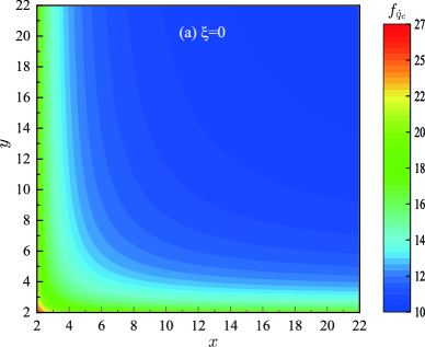
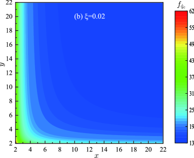
This is a monotonically decreasing function of time durations ($x$ and $y$) of system-bath interaction intervals, both for adiabatic and nonadiabatic driving [see Figs. 2(a) and 2(b)].

Figure 2: Contour plots of relative heat variance, $f_{\dot{q}_{c}}$ in the effective time duration $(x,y)$ plane for an adiabatic ($a$) and nonadiabatic ($b$) driving, with $\xi=0$ and $\xi=0.02$, respectively. The values of the parameters are $\beta_{h}=0.8$, $\beta_{c}=1$, $\omega_{c}=0.6$, and $\omega_{h}=1$.

If the isochoric hot (or cold) branch is completed in an finite time $\tau_{c}$ (or $\tau_{h}$), with finite value of $x_{c}$ (or $x_{h}$), this isochoric step is out of equilibrium and the fluctuations are inevitably avoidable. In order to decrease the relative fluctuations, we thus need to slow down the machine, which, however, must make the average cooling rate $\langle\dot{q}_{c}\rangle$ down. Comparison between 2(a) and 2(b) also shows that the relative fluctuations are larger in nonadiabatic driving with finite time ($\tau_{hc}$ or $\tau_{ch}$) than in adiabatic, quasistatic evolution.

Since no work is produced in the two isochoric processes, the average total work per cycle is $\langle w_{hc}\rangle+\langle w_{ch}\rangle$, where $\langle w_{hc}\rangle=\int w_{hc}p(w_{hc})dw_{hc}$ and $\langle w_{ch}\rangle=\int w_{ch}p(w_{ch},q_{c},w_{hc})$$dw_{hc}dq_{c}dw_{ch}$. It follows, using Eqs. (1) and (5), that the total work can be obtained,

$$\begin{split}\langle w\rangle=2\left(\omega_{h}-\omega_{c}\right)\left[\left(\langle n_{c}\rangle^{eq}+\Delta_{c}\right)-\left(\langle n_{h}\rangle+\Delta_{h}\right)\right]-4\xi\left[\omega_{c}\left(\langle n_{h}\rangle^{eq}+\Delta_{h}\right)+\omega_{h}\left(\langle n_{c}\rangle^{eq}+\Delta_{c}\right)\right].\end{split}$$ (18)

The thermodynamic coefficient of performance, defined by $\varepsilon_{th}=\langle q_{c}\rangle/\langle w\rangle$, is the given by

$$\varepsilon_{th}=\frac{\omega_{c}}{\omega_{h}\frac{1-\xi\mathcal{F}}{1+\xi\mathcal{G}}-\omega_{c}},$$ (19)

where $\mathcal{F}=2(\langle n_{c}\rangle^{eq}+\Delta_{c})/[(\langle n_{c}\rangle+\Delta_{c})-(\langle n_{h}\rangle^{eq}+\Delta_{h})]$ and $\mathcal{G}=2(\langle n_{h}\rangle^{eq}+\Delta_{h})/[(\langle n_{c}\rangle+\Delta_{c})-(\langle n_{h}\rangle^{eq}+\Delta_{h})]$. As $\mathcal{F,G}<0$ and $\xi\geq 0$, the thermodynamic coefficient of performance $\varepsilon_{th}$ increases as the adiabacity parameter $\xi$ decreases, and it reaches its upper bound $\varepsilon_{th}^{ad}=\omega_{c}/(\omega_{h}-\omega_{c})$ in the ideal adiabatic case when $\xi=0$. The fact that the additional heat is dissipated into the hot reservoir due to finite time realization of the compression or expansion, so that the additional work is input to overcome such heat loss, suggests that cycles consisting of nonadiabatic transformation along the expression and compression runs less efficiently than those with ideal adiabatic strokes. While the stochastic COP is defined by $\varepsilon=q_{c}/(w_{hc}+w_{ch})$, its probability distribution $p(\varepsilon)$ can be determined by $p(\varepsilon)=\int\int\int dw_{hc}d{q_{c}}d{w_{hc}}p(w_{ch},q_{c},w_{hc})\delta\left(\varepsilon-\frac{q_{c}}{w_{hc}+w_{ch}}\right)$ to arrive at

$$\begin{split}p\left(\varepsilon\right)=&2\left\{\left[\frac{1}{4}+\left(\langle n_{h}\rangle+\Delta_{h}\right)\left(\langle n_{c}\rangle+\Delta_{c}\right)\right]\left(1-\xi\right)^{2}+\left[\frac{1}{4}-\left(\langle n_{h}\rangle^{eq}+\Delta_{h}\right)\left(\langle n_{c}\rangle^{eq}+\Delta_{c}\right)\right]\xi^{2}\right\}\delta\left(\varepsilon\right)\\ &+2\left[\frac{1}{4}+\left(\langle n_{h}\rangle^{eq}+\Delta_{h}\right)\left(\langle n_{c}\rangle+\Delta_{c}\right)\right]\xi^{2}\delta\left(\varepsilon+\frac{\varepsilon_{th}^{ad}}{2\varepsilon_{th}^{ad}+1}\right)\\ &+2\left[\frac{1}{4}-\left(\langle n_{h}\rangle^{eq}+\Delta_{h}\right)\left(\langle n_{c}\rangle^{eq}+\Delta_{c}\right)\right]\left(1-\xi\right)^{2}\delta\left(\varepsilon-\varepsilon_{th}^{ad}\right)\\ &+\left(1-\xi\right)\xi\left[\delta\left(\varepsilon+1\right)+\delta\left(\varepsilon\right)\right]\end{split}$$ (20)

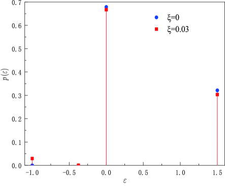
Figure 3: The probability distribution $p(\varepsilon)$ of the quantum stochastic COP for both adiabatic (blue dots) and nonadiabatic (red squares) driving. We observe the appearance of peaks at negative COP in the nonadiabatic case.

We examine the statistics of stochastic COP in Fig. 3 at different $\xi$ for given time durations allocated to the two isochoric strokes ($x$ and $y$). The statistics of COP depends on the adiabacity parameter $\xi$ determined merely by the driving time ($\tau_{hc}$ or $\tau_{ch}$). For adiabatic driving with $\xi=0$ (blue squares), the stochastic COP may be zero or equal to the adiabatic value $\varepsilon_{th}^{ad}$, with the largest peak at zero and the second largest at $\varepsilon_{th}^{ad}$. By contrast, for nonadiabatic driving with $\xi>0$ (red dots), the negative values [$-{\varepsilon_{th}^{ad}}/{(2\varepsilon_{th}^{ad}+1)}$ and $-1$] of $p(\varepsilon)$ are visible due to quantum determinacy, in addition to nonnegative ones (zero and $\varepsilon_{th}^{ad}$). Unlike in a quantum heat engine Lutz20 where the stochastic efficiency can not be defined for $\xi>0$, for the quantum refrigerator the average COP $\langle\varepsilon\rangle$ converges and can thus be well defined.

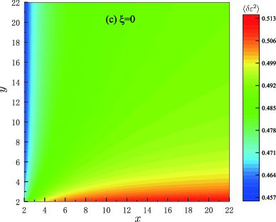
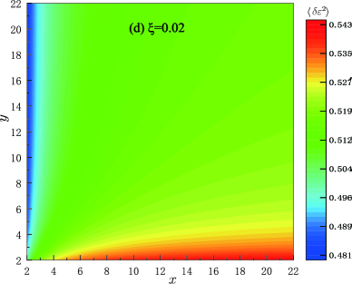
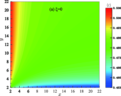
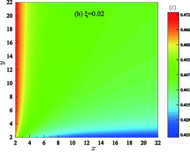
Figure 4: Contour plots of the average COP $\langle\varepsilon\rangle$ and its variance $\langle\delta\varepsilon^{2}\rangle$ in the effective time duration $(x,y)$ plane for an adiabatic ($a$ and $c$) and nonadiabatic ($b$ and $d$) driving, with $\xi=0$ and $\xi=0.02$, respectively. The values of the parameters are $\beta_{h}=0.8$, $\beta_{c}=1$, $\omega_{c}=0.6$, and $\omega_{h}=1$.

Using the distribution function (20), we find that the first two central moments are

$$\begin{split}\langle\varepsilon\rangle=&2\left[\frac{1}{4}-\left(\langle n_{h}\rangle+\Delta_{h}\right)\left(\langle n_{c}\rangle^{eq}+\Delta_{c}\right)\right]\left(1-\xi\right)^{2}\varepsilon_{th}^{ad}\\ &-2\left[\frac{1}{4}+\left(\langle n_{h}\rangle^{eq}+\Delta_{h}\right)\left(\langle n_{c}\rangle^{eq}+\Delta_{c}\right)\right]\xi^{2}\frac{\varepsilon_{th}^{ad}}{2\varepsilon_{th}^{ad}+1}-\left(1-\xi\right)\xi\end{split}$$ (21)

and $\langle\varepsilon^{2}\rangle\!=2\left[\frac{1}{4}-\left(\langle n_{h}\rangle+\Delta_{h}\right)\left(\langle n_{c}\rangle+\Delta_{c}\right)\right]\left(1-\xi\right)^{2}\left(\varepsilon_{th}^{ad}\right)^{2}\!+2\left[\frac{1}{4}+\left(\langle n_{h}\rangle^{eq}+\Delta_{h}\right)\left(\langle n_{c}\rangle^{eq}+\Delta_{c}\right)\right]\xi^{2}\left[{\varepsilon_{th}^{ad}}/({2\varepsilon_{th}^{ad}+1})\right]^{2}+\left(1-\xi\right)\xi.$ This, combining with Eq. (21), gives rise to the variance of stochastic COP, $\delta\varepsilon^{2}=\langle\varepsilon^{2}\rangle-\langle\varepsilon\rangle^{2}$, leading to

$$\begin{split}\delta\varepsilon^{2}=&2\left[\frac{1}{4}-\left(\langle n_{h}\rangle+\Delta_{h}\right)\left(\langle n_{c}\rangle^{eq}+\Delta_{c}\right)\right]\left(1-\xi\right)^{2}\left(\varepsilon_{th}^{ad}\right)^{2}\\ &+2\left[\frac{1}{4}+\left(\langle n_{h}\rangle^{eq}+\Delta_{h}\right)\left(\langle n_{c}\rangle^{eq}+\Delta_{c}\right)\right]\xi^{2}\left(\frac{\varepsilon_{th}^{ad}}{2\varepsilon_{th}^{ad}+1}\right)^{2}\\ &-\big{\{}\xi\left(1-\xi\right)+\left(1-\xi\right)^{2}\left[2\left(\langle n_{h}\rangle+\Delta_{h}\right)\left(\langle n_{c}\rangle^{eq}+\Delta_{c}\right)-\frac{1}{2}\right]\varepsilon_{th}^{ad}\\ &+\xi^{2}\frac{\left[2\left(\langle n_{h}\rangle^{eq}+\Delta_{h}\right)\left(\langle n_{c}\rangle^{eq}+\Delta_{c}\right)+\frac{1}{2}\right]\varepsilon_{th}^{ad}}{2\varepsilon_{th}^{ad}+1}\big{\}}^{2}+\xi\left(1-\xi\right).\end{split}$$ (22)

For a cycle with either adiabatic or nonadiabatic driving branches, the average COP $\langle\varepsilon\rangle$ increases as time duration $y=e^{\gamma_{c}\tau_{c}}$ increases, but it decreases as time duration $x=e^{\gamma_{h}\tau_{h}}$ increases, see Figs. 4(a) and 4(b). This follows from the fact that, for the machine with adiabatic or nonadiabatic processes, the heat absorbed by the system along the cold isochoric stroke increases as $y$ increases, and the heat released to the hot reservoir increases as $x$ increases. Figures 4(c) and 4(d) show that, in contrast to $\langle\varepsilon\rangle$, the variance $\langle\delta\varepsilon^{2}\rangle$ increases as $x$ increases but decreases as $y$ increases, thereby confirming that there is trade-off between average $\langle\varepsilon\rangle$ and the COP fluctuations $\langle\delta\varepsilon^{2}\rangle$. We also observe that the internal dissipation along the adiabats results in performance deterioration for the machine by reducing the average COP $\langle\varepsilon\rangle$ but increasing fluctuations of COP $\langle\delta\varepsilon^{2}\rangle$.

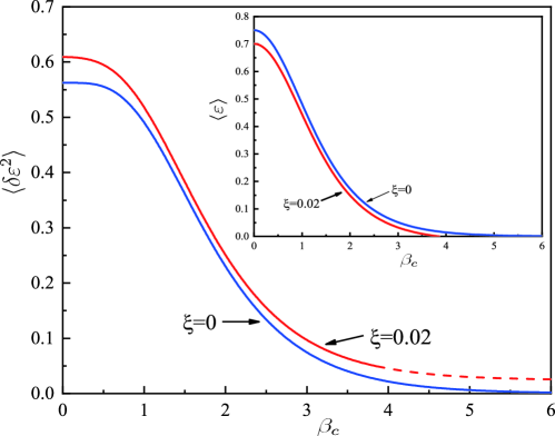
Figure 5: (Color online) The variance of stochastic COP, $\langle\delta\varepsilon^{2}\rangle$, and average COP $\langle\varepsilon\rangle$ (inset) as a function of the inverse temperature of cold reservoir $\beta_{c}=0.8\beta_{h}$ for $\xi=0$ (blue lines) and $\xi=0.02$ (red lines). The red dashed line corresponds to the variance $\langle\delta\varepsilon^{2}\rangle$ in the region of nonphysical, negative mean COP. The parameters are $x=y=20$, $\omega_{c}=0.6$, and $\omega_{h}=1$.

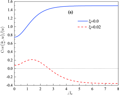
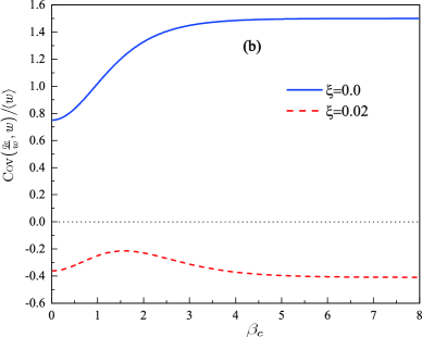
Figure 6: (Color online) The ratio ${\mathrm{Cov}\!\left(\frac{q_{c}}{w},w\right)\!\big{/}\!\langle w\rangle}$ as a function of inverse temperature $\beta_{c}$ as a function of the inverse temperature of cold reservoir $\beta_{c}=0.8\beta_{h}$ for $x=y=20$ (a) and $x=y=2$ (b), where $\xi=0$ and $\xi=0.02$ are indicated by blue lines and red ones, respectively. The other parameters are $\omega_{c}=0.6$ and $\omega_{h}=1$.

For given time durations ($x$ and $y$) of two isochoric processes, both the average and the variance of the stochastic COP as a function of the inverse temperature $\beta_{c}$ of cold reservoir is shown in Fig. 5. When decreasing inverse temperature, both $\langle\varepsilon\rangle$ and $\langle\delta\varepsilon^{2}\rangle$ grow, and as expected, $\langle\delta\varepsilon^{2}\rangle$ would vanish and $\langle\varepsilon\rangle$ would be even negative in the low temperature limit. The non-positive mean COP in the low-temperature regime can be understood that the stochastic COP may be negative due to quantum indeterminacy dominating at low temperatures (see also Fig. 3). While the low temperature domain is characterized by quantum fluctuations, the high temperature region is dominated by larger thermal fluctuations. Therefore, the variance $\langle\delta\varepsilon^{2}\rangle$ gets increased while the temperature is increasing and vice versa.

As the covariance between the total stochastic work $w$ and stochastic COP $\varepsilon$ can be defined by Hei99

$$\mathrm{Cov}\left(\frac{q_{c}}{w},w\right)=(\varepsilon_{th}-\langle\varepsilon\rangle)\langle w\rangle,$$ (23)

the difference between the thermodynamic COP $\varepsilon_{th}$ and average COP $\langle\varepsilon\rangle$ is determined according to $\varepsilon_{th}-\langle\varepsilon\rangle=\mathrm{Cov}\left(\frac{q_{c}}{w},w\right)/\langle w\rangle$. The ratio ${\mathrm{Cov}\!\left(\frac{q_{c}}{w},w\right)\!\big{/}\!\langle w\rangle}$ as a function of inverse temperature $\beta_{c}$ is plotted in Figs. 6(a) and 6(b), where the time durations along two isochores are $x=y=20$ and $x=y=2$, respectively. We notice that, for $\xi=0$ the ratio monotonically increases with increasing inverse temperature. It is moreover always positive, for either fast or slow isochoric branch, indicating that the thermodynamic COP $\varepsilon_{th}$ must be lager than the average COP $\langle\varepsilon\rangle$. By contrast, this ratio increases and then decreases as the temperature is lowered for $\xi>0$. As this ratio can be either positive or negative, the thermodynamic COP $\varepsilon_{th}$ can be larger or smaller than the corresponding average COP $\langle\varepsilon\rangle$ for nonadiabatic driving.

IV Conclusion

In summary, we have developed a general scheme allowing to determine statistics of cooling rate and COP for a quantum Otto refrigerator by analyzing the time evolution of the two isochores and two adiabats. These performance parameters as well as their statistics are determined by the finite time durations required for completing the two nonadiabatic driving strokes and two isochoric branches with incomplete thermalization. When treating an analytically solvable two-level engine, we find that stochastic COP may be negative due to quantum indeterminacy, and but its average value converges and can thus be well defined. We show that there is trade-off between these variables and their corresponding fluctuations at zero and finite temperature, thereby indicating that the price for enhancing the machine performance is increasing fluctuations. We have additionally compared the average COP and the conventional thermodynamic COP, and we found that they are positive correlated for ideal adiabatic strokes, but their correlation may be negative for nonadibatic branches.

Appendix A Time evolution of population along an isochoric process

When a system under external control is weakly coupled to a heat reservoir, the quantum dynamics of the system generated by both thermal interaction and external fields can be described by a semigroup approach. The change in time of an operator $\hat{X}$ for a system with Hamiltonian $\hat{H}$ is determined according to the master equation Fel00 ; Wang19 :

$$\frac{d{\hat{X}}}{dt}=i[\hat{H},~{}\hat{X}]+\frac{\partial{\hat{X}}}{\partial t}+\mathcal{L}_{D}(\hat{X}),$$ (A.1)

where

$$\mathcal{L}_{D}(\hat{X})=\sum_{\alpha}k_{\alpha}\left(\hat{V}_{\alpha}^{\dagger}\left[\hat{X},\hat{V}_{\alpha}^{\dagger}\right]+\left[\hat{V}_{\alpha}^{\dagger},\hat{X}\right]\hat{V}_{\alpha}\right)$$ (A.2)

is the Liouville dissipative generator due to the system-reservoir thermal interaction. $\hat{V}_{\alpha}$ are operators in the Hilbert space of the system and $\hat{V}_{\alpha}^{\dagger}$ are Hermitian conjugates, and $k_{\alpha}$ are phenomenological positive coefficients. In Eq. (A.2), $[\hat{X},\hat{V}_{\alpha}^{\dagger}]=[\hat{X},\hat{V}_{\alpha}^{\dagger}]_{-}$ denotes commutator for the Bose system, and $[\hat{X},\hat{V}_{\alpha}^{\dagger}]=[\hat{a},\hat{b}]_{+}$ is used for anticommutator for the Fermi system. Substituting $\hat{X}=\hat{H}$ into Eq. (A.1) leads to

$$\left\langle\frac{d\hat{H}}{dt}\right\rangle={\left\langle\frac{\partial{\hat{H}}}{\partial t}\right\rangle}+\langle\mathcal{L}_{D}(\hat{H})\rangle.$$ (A.3)

This reproduces the time derivative of quantum version of the first law of thermodynamics ${d\langle\hat{H}\rangle}/{dt}={{\mathchar 22\relax\mkern-12.0mud}{\langle w\rangle}}/{dt}+{{\mathchar 22\relax\mkern-12.0mud}{\langle q\rangle}}/{dt}$, when the instantaneous average power and the average heat current are identified as, ${{\mathchar 22\relax\mkern-12.0mud}{\langle w\rangle}}/{dt}={\langle{\partial{\hat{H}}}/{\partial t}\rangle}$ and ${{\mathchar 22\relax\mkern-12.0mud}{\langle q\rangle}}/{dt}=\langle\mathcal{L}_{D}(\hat{H})\rangle$, respectively.

To proceed, we choose the operators $\hat{V}^{\dagger}$ and $\hat{V}$ as the bosonic (fermionic) creation operator $\hat{a}^{\dagger}$ and annihilation operator $\hat{a}$ for the Bose (Fermi) system. Inserting the system Hamiltonian $\hat{H}=\omega\hat{a}^{\dagger}\hat{a}$ into Eq. (A.1) and taking the expectation value, the motion of the population $\langle n\rangle=\langle a^{\dagger}a\rangle$ along an isochoric process with constant $\omega$ can be obtained as

$$\frac{d\langle n\rangle}{dt}=-\gamma(\langle n\rangle-\langle{n}\rangle^{eq}),$$ (A.4)

where $\gamma=k_{\downarrow}-{k_{\uparrow}}~{}(\gamma=k_{\downarrow}+{k_{\uparrow}})$ denotes the thermal conductivity for the Bose (Fermi) system. The detailed balance $k_{\uparrow}=k_{\downarrow}e^{-\beta\hbar\omega}$ is assumed to be satisfied, ensuring that the system can achieve asymptotically the thermal state after an infinitely long system-bath interaction duration. Here ${\langle n\rangle}^{eq}=\frac{1}{2}\frac{k_{\downarrow}+k_{\uparrow}}{k_{\downarrow}-{k_{\uparrow}}}$ $\left(\langle n\rangle^{eq}=\frac{1}{2}\frac{k_{\downarrow}-k_{\uparrow}}{k_{\downarrow}+{k_{\uparrow}}}\right)$ is the asymptotic value of $\langle n(t)\rangle$ with $t\rightarrow\infty$, and it corresponds to the equilibrium population: $\langle{n}\rangle=1/(e^{\beta\omega}-1)$ [$\langle n\rangle=-\frac{1}{2}\tanh(\beta\omega/2)$]. From Eq. (A.4), we find that instantaneous population $\langle n(t)\rangle$ along the thermalization process (staring at initial time $t=0$) can be written in terms of the population $\langle n(0)\rangle$,

$$\langle{n}(t)\rangle=\langle n\rangle^{eq}+[\langle n(0)\rangle-\langle n\rangle^{eq}]e^{-\gamma t}.$$ (A.5)

Appendix B Relation between populations at the begin and the end of a unitary driving process

We consider the unitary time evolution along the unitary adiabatic expansion $A\rightarrow B$ to identify the explicit relation of the populations at $A$ and $B$. For a two level system, its eigenenergies are $E_{+}=\frac{1}{2}\hbar\omega$, and $E_{-}=-\frac{1}{2}\hbar\omega$. The partition function at the initial instant $A$ along this process can be given by

$$Z_{A}=e^{-\beta_{A}\hbar\omega_{h}/2}+e^{\beta_{A}\hbar\omega_{h}/2}=2\cosh\left(\frac{\beta_{A}\hbar\omega_{h}}{2}\right),$$ (B.1)

which, together with the occupation probabilities $p_{+}=e^{-\beta\hbar\omega_{h}/2}/Z_{A}$ and $p_{-}=e^{\beta\hbar\omega_{h}/2}/Z_{A}$, gives the population at instant $A$,

$$\langle n_{A}\rangle=\frac{1}{2Z_{A}}\left(e^{-\beta\hbar\omega_{h}/2}-e^{\beta\hbar\omega_{h}/2}\right)=-\frac{1}{2}\tanh\left(\frac{\beta\hbar\omega_{h}}{2}\right).$$ (B.2)

The average population at instant $B$ can then be determined according to

$$\begin{split}\langle n_{B}\rangle&=\sum_{n,m}mp_{n\rightarrow m}^{\tau_{hc}}p_{n}^{0}(A)\\ &=\sum_{n,m}m|\langle n|U_{\mathrm{exp}}|m\rangle|^{2}p_{n}^{0}(A)\\ &=\frac{1}{Z_{A}}\big{[}e^{-\beta_{A}\omega_{h}/2}\left(|\langle+|U_{\mathrm{exp}}|+\rangle|^{2}-\langle+|U_{\mathrm{exp}}|-\rangle|^{2}\right)\\ &+e^{\beta_{A}\omega_{h}/2}\left(|\langle-|U_{\mathrm{exp}}|+\rangle|^{2}-\langle-|U_{\mathrm{exp}}|-\rangle|^{2}\right)\big{]}\\ &=\frac{1}{Z_{A}}\left[e^{-\beta_{A}\omega_{h}/2}\left(1-2\xi\right)+e^{\beta_{A}\omega_{h}/2}\left(2\xi-1\right)\right]\\ &=\left(1-2\xi\right)\langle n_{A}\rangle\end{split}$$ (B.3)

where $\xi=|\langle\pm|U_{\mathrm{exp}}|mp\rangle|^{2}$ and $\langle n_{A}\rangle$ was defined in Eq. (B.2). As for the two-level system $\langle n_{B}\rangle<0$, $\xi$ must be upper limited by $1/2$. Similarly, for the unitary compression $C\rightarrow D$, we have

$$\langle n_{D}\rangle=(1-2\xi)\langle n_{C}\rangle.$$ (B.4)

where $\xi=|\langle\pm|U_{\mathrm{com}}|\mp\rangle|^{2}$.

Acknowledgements This work is supported by National Science Foundation of China (Grant Nos. 11875034 and 11505091), and by the State Key Program of China under Grant NO. 2017YFA0304204. J. H. W. also acknowledges the financial support from the Major Program of Jiangxi Provincial Natural Science Foundation (Grant No. 20161ACB21006).

References

• (1) T. Feldmann and R. Kosloff, Quantum four-stroke heat engine: Thermodynamic observables in a model with intrinsic friction, Phys. Rev. E 68, 016101 (2003); T. Feldmann and R. Kosloff, Performance of discrete heat engines and heat pumps in finite time, Phys. Rev. E 61, 4774 (2000).
• (2) Y. Rezek and R. Kosloff, Irreversible Performance of a Quantum Harmonic Heat Engine, New J. Phys. 8, 83 (2006).
• (3) S. H. Su, X. Q. Luo, J. C. Chen and C. P. Sun. Angle-dependent quantum Otto heat engine based on coherent dipole-dipole coupling. Europhy. Lett. 115, 30002 (2016).
• (4) Y. Hong, Y. Xiao, J. He, and J. H. Wang, Quantum Otto engine working with interacting spin systems: Finite power performance in stochastic thermodynamics, Phys. Rev. E 102, 022143 (2020).
• (5) O. Abah, J. Roßnagel, G. Jacob, S. Deffner, F. Schmidt-Kaler, K. Singer, and E. Lutz, Single ion heat engine with maximum efficiency at maximum power, Phys. Rev. Lett. 109, 203006 (2012).
• (6) H. Quan, H., Y. -X. Liu, C. P. Sun, F. Nori, Quantum thermodynamic cycles and quantum heat engines, Phys. Rev. E 76, 031105 (2007).
• (7) R. J. de Assis, T. M. de Mendonça, C. J. Villas-Boas, A. M. de Souza, R. S. Sarthour, I. S. Oliveira, and N. G. de Almeida, Efficiency of a Quantum Otto Heat Engine Operating under a Reservoir at Effective Negative Temperatures, Phys. Rev. Lett. 122, 240602 (2019).
• (8) R. Kosloff and A. Levy, Quantum heat engines and refrigerators: Continuous devices, Annu. Rev. Phys. Chem. 65, 365 (2014).
• (9) B. Cleuren, B. Rutten, and C. Van den Broeck, Phys. Rev. Lett. 108, 120603 (2012).
• (10) F. Tonner, G. Mahler, Autonomous quantum thermodynamic machines. Phys. Rev. E 72(6), 066118 (2005).
• (11) N. Linden, S. Popescu, and P. Skrzypczyk, How small can thermal machines be? the smallest possible refrigerator. Phys. Rev. Lett., 105(13), 130401 (2010).
• (12) A. Levy, and R. Kosloff, Quantum absorption refrigerator, Phys. Rev. Lett. 108, 070604 (2012).
• (13) G. Maslennikov, S. Ding, R.Hablützel, J. Gan, A. Roulet, S. Nimmrichter, J. Dai, V.Scarani, and D. Matsukevich, Quantum absorption refrigerator with trapped ions , Nature Commun. 10, 202 (2019).
• (14) A. Alecce, F. Galve, N. Lo Gullo, L. Dell' Anna, F. Plastina, and R. Zambrini, Quantum Otto cycle with inner friction: finite-time and disorder effects, New J. Phys. 17, 075007 (2015).
• (15) S. Lee, M .Ha, J. M. Park, and H. Jeong, Finite-time quantum Otto engine: Surpassing the quasistatic efficiency due to friction, Phys. Rev. E 101, 022127 (2020).
• (16) C. de Tomas, A. C. Hernandez, and J. M. M. Roco, Phys. Rev. E 85, 010104(R) (2012).
• (17) Y. Wang, M. Li, Z. C. Tu, A. C. Hernandez, and J. M. M. Roco, Phys. Rev. E 86, 011127 (2012).
• (18) Y. Hu, F. Wu, Y. Ma, J. Z. He, J. H. Wang, A. Calvo Hernández, and J. M. M. Roco, Coefficient of performance for a low-dissipation Carnot-like refrigerator with nonadiabatic dissipation, Phys. Rev. E 88, 062115 (2013).
• (19) Y. Izumida, K. Okuda, J. M. M. Roco, and A. Calvo Hernández, Heat devices in nonlinear irreversible thermodynamics Phys. Rev. E 91, 052140 (2015).
• (20) U. Seifert, Stochastic thermodynamics, fluctuation theorems and molecular machines, Rep. Prog. Phys. 75, 126001 (2012).
• (21) K. Sekimoto, Stochastic Energetics (Spinger, Berlin, 2010).
• (22) M. Esposito, U. Harbola and S. Mukamel, Nonequilibrium fluctuations, fluctuation theorems, and counting statistics in quantum systems, Rev. Mod. Phys. 81, 1665 (2009).
• (23) M. Campisi, P. Hänggi, and P. Talkner, Quantum fluctuation relations: Foundations and applications, Rev. Mod. Phys. 83, 771 (2011).
• (24) P. Solinas, D. V. Averin, and J. P. Pekola, Work and its uctuations in a driven quantum system, Phys. Rev. B 87, 060508(R) (2013).
• (25) F. W. J. Hekking and J. P. Pekola, Quantum jump approach for work and dissipation in a two-level system, Phys. Rev. Lett. 111, 093602 (2013).
• (26) T. B. Batalhão, A. M. Souza, L. Mazzola, R. Auccaise, R. S. Sarthour, I. S. Oliveira, J. Goold, G. De Chiara, M. Paternostro, and R. M. Serra, Experimental reconstruction of work distribution and study of uctuation relations in a closed quantum system, Phys. Rev. Lett. 113, 140601 (2014).
• (27) G. Verley, C. Van den Broeck, and M. Esposito, Work statistics in stochastically driven systems, New J. Phys. 16, 095001 (2014).
• (28) Y. Qian, and F. Liu, Computing characteristic functions of quantum work in phase space Physical Review E 100, 062119 (2019).
• (29) Z. Fei, N. Freitas, V. Cavina, H. T. Quan, and M. Esposito, Work statistics across a quantum phase transition, Phys. Rev. Lett 124, 170603 (2020).
• (30) F. Cerisola, Y. Margalit, S. Machluf, A. J. Roncaglia, J. P. Paz, and R. Folman, Using a quantum work meter to test non-equilibrium uctuation theorems, Nat. Commun. 8, 1241 (2017).
• (31) S. Rahav, U. Harbola, and S. Mukamel, Heat fluctuations and coherences in a quantum heat engine, Phys. Rev. A 86, 043843 (2012).
• (32) T. Denzler and E. Lutz, Heat distribution of a quantum harmonic oscillator, Phys. Rev. E 98, 052106 (2018).
• (33) S. Gasparinetti, P. Solinas, A. Braggio, and M. Sassetti, Heat-exchange statistics in driven open quantum systems, New J. Phys. 16, 115001 (2014).
• (34) V. Holubec and A. Ryabov, Cycling Tames Power Fluctuations Near Optimum Efficiency, Phys. Rev. Lett. 121, 120601 (2018).
• (35) V. Holubec, An exactly solvable model of a stochastic heat engine: Optimization of power, power fluctuations and efficiency, J. Stat. Mech. P05022 (2014).
• (36) J. H. Wang, J. Z. He, and Y. L. Ma, Finite-time performance of a quantum heat engine with a squeezed thermal bath, Phys. Rev. E 100, 052126 (2019).
• (37) T. Denzler and E. Lutz, Efficiency fluctuations of a quantum heat engine, Phys. Rev. Research 2, 032062 (2020).
• (38) H. Vroylandt, A. Bonfils, and G. Verley, Efficiency fluctuations of small machines with unknown losses, Phys. Rev. E 93, 052123 (2016).
• (39) J.-M. Park, H.-M. Chun and J. D. Noh, Efficiency at maximum power and efficiency fluctuations in a linear Brownian heat-engine model, Phys. Rev. E 94, 012127 (2016).
• (40) G. Verley and M. Esposito, Efficiency statistics at all times: Carnot limit at finite power M Polettini, Phys. Rev. Lett. 114, 050601 (2015).
• (41) G. Verley, T Willaert, C. Van den Broeck, and M. Esposito, Universal theory of efficiency fluctuations, Phys. Rev.E 90, 052145 (2014).
• (42) H. Vroylandt, M. Esposito, and G. Verley, Efficiency fluctuations of stochastic machines undergoing a phase transition, Phys. Rev. Lett. 124, 250603 (2020).
• (43) J. -H. Jiang, B. K. Agarwalla, and D. Segal, Efficiency Statistics and Bounds for Systems with Broken Time-Reversal Symmetry, Phys. Rev. Lett. 115, 040601 (2015).
• (44) P. Talkner, E. Lutz, and P. Hänggi, Fluctuation theorems: Work is not an observable, Phys. Rev. E 75, 050102 (2007).
• (45) M. Born and V. Fock, Z. Phys. 51, 165 (1928).
• (46) Plastina, F. A. Alecce, T.J.G. Apollaro, G. Falcone, G. Francica, F. Galve, N. Lo Gullo, and R. Zambrini. Irreversible work and inner friction in quantum thermodynamic processes. Phys. Rev. Lett. 113, 260601 (2014).
• (47) L. A. Correa, J. P. Palao, and D. Alonso, Internal dissipation and heat leaks in quantum thermodynamic cycles, Phys. Rev. E 92, 032136 (2015).
• (48) P. A. Camati, J. F. G. Santos, and R. M. Serra, Coherence effects in the performance of the quantum Otto heat engine, Phys. Rev. A 99, 062103 (2019).
• (49) R. Heijmans, When does the expectation of a ratio equal the ratio of expectations?, Statistical Papers 40, 107 (1999).