Frequency Consistent Adaptation for Real World Super Resolution

Abstract

Recent deep-learning based Super-Resolution (SR) methods have achieved remarkable performance on images with known degradation. However, these methods always fail in real-world scene, since the Low-Resolution (LR) images after the ideal degradation (e.g., bicubic down-sampling) deviate from real source domain. The domain gap between the LR images and the real-world images can be observed clearly on frequency density, which inspires us to explictly narrow the undesired gap caused by incorrect degradation. From this point of view, we design a novel Frequency Consistent Adaptation (FCA) that ensures the frequency domain consistency when applying existing SR methods to the real scene. We estimate degradation kernels from unsupervised images and generate the corresponding LR images. To provide useful gradient information for kernel estimation, we propose Frequency Density Comparator (FDC) by distinguishing the frequency density of images on different scales. Based on the domain-consistent LR-HR pairs, we train easy-implemented Convolutional Neural Network (CNN) SR models. Extensive experiments show that the proposed FCA improves the performance of the SR model under real-world setting achieving state-of-the-art results with high fidelity and plausible perception, thus providing a novel effective framework for real-world SR application.

Introduction

Super-Resolution (SR) is a basic low-level visual problem (Freeman, Jones, and Pasztor 2002; Glasner, Bagon, and Irani 2009), which is defined as enlarging the resolution of a Low-Resolution (LR) image and restoring it to a High-Resolution (HR) image. In recent years, deep-learning methods have dominated the research in the SR field, and lots of novel structures (Dong et al. 2015; Tai et al. 2017; Chen et al. 2018; Tai, Yang, and Liu 2017; Lai et al. 2017; Kim, Kwon Lee, and Mu Lee 2016; Lim et al. 2017) are proposed to improve performance on standard benchmarks. However, known degradation used to train these models is not suitable to real-world scenarios. In fact, the SR model is sensitive to different degradation (Zhang, Zuo, and Zhang 2019; Zhou and Susstrunk 2019; Gu et al. 2019). Inconsistent degradation leads to generating undesirable SR results, either losing high-frequency detail or producing artifacts.

Figure 1: $\mathbf{4\times}$ SR results of different methods on a real image taken by smartphone. The red rectangle area of each result is cropped and enlarged for visual comparison. Compared with other results, our method generates natural HR image without blur or artifacts.

To address the challenge of Real-World Super-Resolution (RWSR), some non-blind/blind SR methods have been proposed to improve SR performance under real degradation. Among them, ZSSR (Shocher, Cohen, and Irani 2018) explores the internal information inside the image and uses the zero-shot learning method by training on the test image. However, the given kernel is needed when constructing training pairs, which is not available in real scene. IKC (Gu et al. 2019) tries to construct supervised data and predict the degraded kernel from LR images. However, the supervised training is not suitable for real-world scene due to the lack of ground-truth blur kernel that can be obtained. KernelGAN (Bell-Kligler, Shocher, and Irani 2019) utilizes the prior of recurrent patches across scales in natural LR images to train a deep linear network, whose convolution kernels can be calculated to obtain the estimated kernel. However, its insufficient recurrent patch prior and complex implementation with manual constraints limit its accuracy.

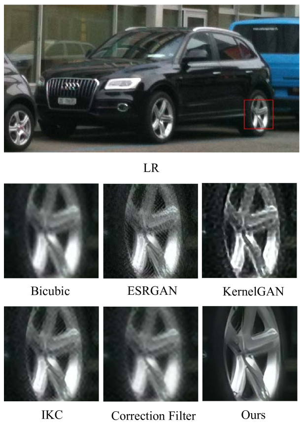
To better deal with RWSR, we propose a novel method named Frequency Consistent Adaptation (FCA). By accurately estimating the degradation inside the source image, our FCA can generate realistic HR-LR image pairs. We design an adaptation generator to learn the blur kernel from the source image, and then degrade the down-sampled LR image. In order to draw the degraded LR image as close as possible to the source domain, we propose a novel Frequency Density Comparator (FDC). The frequency distributions of different degraded images show obvious differences, and their orders motivate us to construct the correspondence between the frequency domain and the blur kernel. FDC can learn embeddings related to frequency density which are essential to distinguish images with different degrees of degradation. Through trained in a self-supervised way, FDC provides effective gradient information for the adaptation generator. By constructing training images consistent to the real degradation, FCA can be combined with existing SR networks to improve their performance. Figure 1 shows an example of our FCA’s performance improvement for real-world SR. Compared with the existing state-of-the-art methods, our result achieves higher visual quality.

In summary, our overall contribution is three-fold:

• We propose a novel frequency consistent adaptation for real-world super-resolution, which guarantees frequency consistency for realistic degradation.

• We carefully design frequency density comparator to provide guidance for accurate blur kernel estimation. Our unsupervised training strategy is flexible for real scene.

• Extensive experiments on various synthetic and real-world datasets show that the proposed FCA achieves state-of-the-art performance.

Related Work

CNN-based Super Resolution

Recently, many Convolutional Neural Networks (CNN) based SR networks (Lim et al. 2017; Pan et al. 2018; He et al. 2019; Hu et al. 2019; Li et al. 2019; Qiu et al. 2019; Yin et al. 2019) achieve strong performance on bicubic down-sampled images. Among them, EDSR (Lim et al. 2017) adopts a deep residual network for training SR model. Zhang (Zhang et al. 2018b) proposes a residual in residual structure to construct very deep network that achieves better performance than EDSR. Haris (Haris, Shakhnarovich, and Ukita 2018) proposes deep back-projection networks to exploit iterative up- and down-sampling layers, providing an error feedback mechanism for projection errors at each stage.

Figure 2: Training and testing pipeline of real-world super-resolution. When applying a SR model to real scene, a typical pipeline includes: 1. Constructing LR-HR pair by performing degradation with a blur kernel. 2. Training a SR model $f$ to reconstruct HR image ${\mathbf{I}}_{HR}$ for each ${\mathbf{I}}_{LR}$. 3. Testing SR model on real-world image.

Figure 3: Illustration of the degradation’s importance in SR. Different blur kernels might get different degraded LR images, resulting in different SR models. For a degradation-unknown image ${\mathbf{x}}$, only SR model ($f_{B}$) with a consistent degradation kernel generates natural HR result (Middle row), while those ($f_{A}$ and $f_{C}$) with inconsistent kernels generate over-smoothing (Top row) or over-sharpening (Bottom row) images.

Although these works have achieved good performance with respect to fidelity, the generated images have poor visual effects and appear blurry. To address this issue, some researchers propose to enhance realistic texture via spatial feature transform (Zhang et al. 2019b; Zheng et al. 2018; Wang et al. 2018a). Furthermore, some Generative Adversarial Networks (GAN) based methods (Ledig et al. 2017; Zhang et al. 2019a; Wang et al. 2018b) pay more attention to visual effects, introducing adversarial losses (Goodfellow et al. 2014) and perceptual losses (Johnson, Alahi, and Fei-Fei 2016). Soh (Soh et al. 2019) proposes a natural manifold discrimination to classify HR images with blurry or noisy images, which is used to supervise the quality of the generated images. However, these SR models trained on the data generated by bicubic kernel can only work well on ideal dataset which is inconsistent with real-world needs. In this paper, we proposed to analyse the degradation of real images, and achieve robust performance in real scene.

Real World Super Resolution

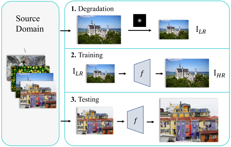
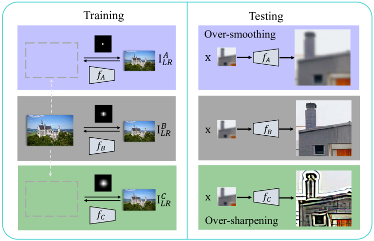
For real-world super-resolution application (Lugmayr, Danelljan, and Timofte 2020; Ji et al. 2020), SR models need to be tested on real scene which is often deviated from ideal domain. To overcome these challenges, recent works with new training strategy have been proposed. Despite the difference in detail, the common strategy of these models for RWSR is described in Figure 2. These methods (Zhou and Susstrunk 2019) are trained on the artificially constructed degraded training pair, which further enhanced the robustness of the SR model. However, the explicit modeling way adopted by these methods needs sufficient prior about degradation, therefore the scope of application is limited. Another problem is that these methods (Zhang, Zuo, and Zhang 2018, 2019) evaluate performance on self-made datasets, which lacks objective and fair comparison on public benchmark datasets. In this work, we mainly focus on kernel estimation, and the noise estimation can be easily introduced as (Ji et al. 2020). We show that different degrees of kernel degradation have a huge impact on the performance of the SR model in Figure 3.

To achieve better performance on real scene images, several recent works considering degradation have been proposed. ZSSR (Shocher, Cohen, and Irani 2018) abandons the training process on external data and train a specific model for each test image with more attention to the internal information of the image. However, as a non-blind model, ZSSR needs given blur kernel, which restricts its applicability. KernelGAN (Bell-Kligler, Shocher, and Irani 2019) propose unsupervised kernel estimation GAN to generate down-sampling kernel. It can be used as given kernel for ZSSR. However, KernelGAN adopts only adversarial loss thus often produces unstable results. IKC (Gu et al. 2019) proposes to explicitly predict blur kernel in an iterative way. The supervised training method only work for synthetic data. Our unsupervised FCA is not limited to synthetic images but also suitable for real-world images. Correction Filter (Hussein, Tirer, and Giryes 2020) modifies the low-resolution image to match one that is obtained by another kernel (e.g., bicubic) and thus improves the results of existing pre-trained CNNs. However, degraded LR often loses important frequency information, which makes it hard to rematch bicubic domain. In contrast, we match the LR domain to source domain without necessary to reconstruct important details. Instead, we encourage CNN models to generate rich high-frequency details in training phase.

Frequency Consistent Adaptation

Problem Formulation

Generally, we assume LR image is obtained from HR image by the following degradation:

$${\mathbf{I}}_{LR}=({\mathbf{I}}_{HR}{\downarrow}_{s})\otimes\mathbf{k}+\mathbf{n},$$ (1)

where ${\mathbf{k}}$ and ${\mathbf{n}}$ indicate blur kernel and noise, respectively. Based on the degraded LR-HR pairs, the ideal SR model for source domain should be:

$$f^{*}=\arg\min_{f}\{\mathbb{E}[\|\mathbf{I}_{HR}-f({\mathbf{I}}_{LR})\|]\},$$ (2)

where $f$ denotes SR model.

Frequency Consistency

Figure 4: (a) Degradation with different blur kernels show difference in frequency density. The frequency is increasing from middle of horizon axis. Domain A/C represents images degraded with small/big variance blur kernel, and it has a strong/weak density in frequency domain. Domain B is a consistent degradation, thus is close to source domain. (b) Impacts of down- and up-sampling on frequency density. Down-sampling on source domain with scale factor $0.5$ might increase frequency density, and up-sampling with $2.0$ impacts the opposite way.

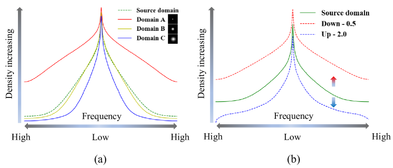
We observe the evidence that frequency density of LR images is related to the corresponding degradation shown in Figure 4 (a). We calculate frequency density as

$$\mathcal{F}_{X}(l) =\frac{1}{N}\Sigma_{x\in X}{|F_{l}(x)|},$$ (3)

where $\mathcal{F}_{X}(l)$ denotes density of frequency $l$ on domain $X$ with $N$ images. We average the two-dimensional Fourier transform along a certain dimension to get $F_{l}(\cdot)$. The relationship between degradation and frequency density motivates us to keep frequency consistency between ${\mathbf{I}}_{LR}$ and source image ${\mathbf{x}}$. We focus on estimating ${\mathbf{k}}$ with frequency domain regularization, which can be formulated as

$${\mathbf{k}}^{*}=\arg\min_{\mathbf{k}}\Phi(({\mathbf{I}}_{HR}{\downarrow}_{s})~{}\otimes{\mathbf{k}},{\mathbf{x}}),$$ (4)

where ${\mathbf{x}}$ indicates image from source domain, and $\Phi$ represents frequency regularization. However, it is hard to directly involve Fourier transform into networks. Guided by the proposed frequency consistency losses, FCA provides LR images that are frequency-consistent with images in source domain $S$. The HR images can be obtained directly from the source images ${\mathbf{x}}\in S$ or by performing down-sampling or deblurring. Those constructed HR-LR training pairs can then be used to train SR models specifically for $S$.

Figure 5: Framework of the proposed frequency consistent adaptation. The adaptation generator takes the unknown degraded image as input, and generates LR image G(x), while the frequency density comparator and the wavelet discriminator provide frequency consistency losses to guide the adaptation generator.

Overall Framework

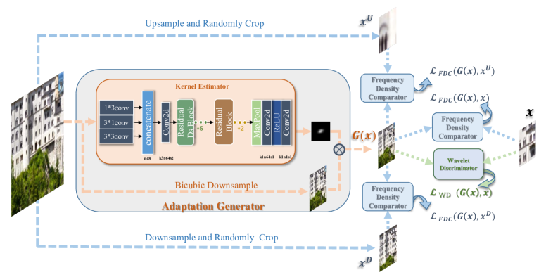
Our FCA shown in Figure 5 consists of three components: the adaptation generator, FDC, and the wavelet discriminator. The adaptation generator generates degraded LR with the same frequency density according to the input image, which is optimized by the guidance of FDC module and the wavelet discriminator module.

Adaptation Generator

For an input source image ${\mathbf{x}}$, the adaptation generator first analyzes the degradation and outputs an anisotropic Gaussian kernel. Then the kernel is convolved with the down-sampled image of ${\mathbf{x}}$ with scale factor $s$ to generate LR image $G(x)$, which is formulated as

$$G(x)=({\mathbf{x}}\downarrow_{s})\otimes{\mathbf{k}}({\mathbf{x}}),$$ (5)

where ${\mathbf{k}}({\cdot})$ means the kernel estimator. More precisely, we describe the estimated kernel with three parameters:

$${\mathbf{k}}({\mathbf{x}})=g(r_{1}({\mathbf{x}}),r_{2}({\mathbf{x}}),\theta({\mathbf{x}})),$$ (6)

where $r_{1}$, $r_{2}$, $\theta$ indicate the horizontal, vertical radius and the angle of rotation respectively. $g(\cdot)$ denotes anisotropic Gaussian kernel.

Frequency Density Comparator

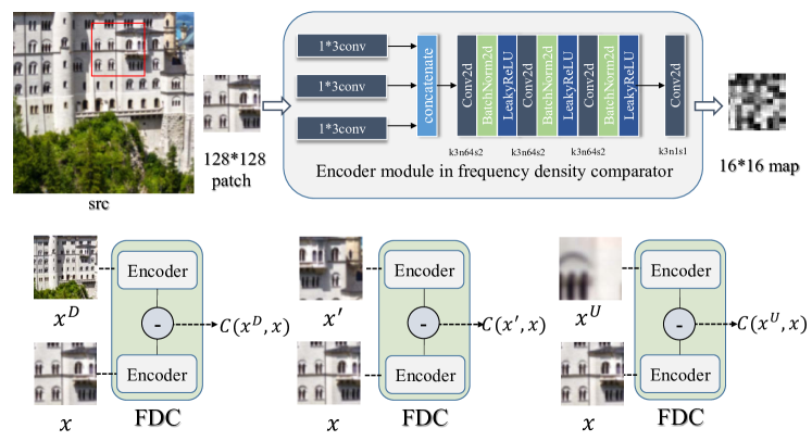
As illustrated in Figure 6, FDC is designed to capture the frequency density relationship of two input patches. For a real image ${\mathbf{x}}$, both down-sampling and up-sampling might change its frequency distribution as shown in Figure 4 (b). The density relations are as follows:

$$C({\mathbf{x}}^{D},~{}{\mathbf{x}}) >0$$ (7)

$$C({\mathbf{x}}^{{}^{\prime}}~{},~{}{\mathbf{x}}) =0$$

$$C({\mathbf{x}}^{U},~{}{\mathbf{x}}) <0$$

where $D$ and $U$ indicate down-sampling and up-sampling respectively. $C$ is the proposed comparator. ${\mathbf{x}}^{{}^{\prime}}$ is another patch from source image. The optimization of $C$ can be formulated as:

$$\arg\min_{C}\{~{}\mathbb{E}_{{\mathbf{x}}\in S}[~{}\|C({\mathbf{x}}^{D},{\mathbf{x}})-1\|$$ (8)

$$+\|C({\mathbf{x}}^{{}^{\prime}},{\mathbf{x}})\|+\|C({\mathbf{x}}^{U},{\mathbf{x}})+1\|~{}]~{}\},$$

where $S$ represents images from source domain. At the beginning, FDC acquires the ability of comparing frequency density on coarse-grain according to the three kinds of patches. To gradually obtain a fine-grained FDC, we dynamically narrow the classification boundary by adjusting the scales of up- and down-sampling during training.

Figure 6: Illustration of our frequency density comparator. FDC has two encoder modules with shared weights. The encoder encodes the two input patches into latent space and outputs the embedding of frequency density. FDC then returns the substruction value of the two embeddings.

Frequency Consistency Loss

FDC provides frequency consistency loss $\mathcal{L}_{FDC}$ for training the generator, which consists of three parts:

$$\mathcal{L}_{FDC} =\mathbb{E}_{{\mathbf{x}}\in S}[~{}\|C(G({\mathbf{x}}),{\mathbf{x}}^{D})+1\|$$ (9)

$$+\|C(G({\mathbf{x}}),{\mathbf{x}})\|+\|C(G({\mathbf{x}}),{\mathbf{x}}^{U})-1\|~{}].$$

$\mathcal{L}_{FDC}$ ensures $G({\mathbf{x}})$ lies between the upper frequency boundary ${\mathbf{x}}^{D}$ and the lower boundary ${\mathbf{x}}^{U}$. Furthermore, the distance measurement between $G({\mathbf{x}})$ and ${\mathbf{x}}$ makes the kernel estimation closer to the real degradation.

Curriculum Learning Strategy

In order to provide stable and accurate gradient information for the adaptation generator, we take the idea of curriculum learning  (Bengio 2013). The training process of frequency density comparator is divided into different stages with increasing difficulty. The up- and down-sampling scale factors of source image for FDC training are set to multiple intermediate values dynamically approaching $1.0$. We train FDC and adaptation generator simultaneously to ensure that the input patches of them share the similar frequency domain for each mini batch.

Wavelet Discriminator

In addition to $\mathcal{L}_{FDC}$, we also use adversarial loss to push LR closer to the source high-frequency domain. Maintaining high-frequency information is very important for recovering image details. We adopt a similar idea with (Fritsche, Gu, and Timofte 2019) and (Wei et al. 2020), imposing adversarial loss only in the high-frequency space. High-frequency and low-frequency components are obtained by wavelet transform, but only the former is input into the discriminator. Since only the non-semantic information of the image needs to be captured, the discriminator network has a shallow depth of only $4$ layers. Moreover, we use LSGAN (Mao et al. 2017) instead of original GAN. Denote the discriminator as $WD$, we optimize it as

$$\arg\min_{WD}\{\mathbb{E}_{{\mathbf{x}}\in S}[(WD(G({\mathbf{x}})))^{2}+(WD({\mathbf{x}})-1)^{2}]\}.$$ (10)

The adversarial loss fed back by the discriminator to the generator can be expressed as:

$$\mathcal{L}_{WD}=\mathbb{E}_{{\mathbf{x}}\in S}[(WD(G({\mathbf{x}}))-1)^{2}],$$ (11)

where $\mathcal{L}_{WD}$ denotes the wavelet discriminator loss.

Overall Loss

As mentioned above, the overall loss $L_{total}$ contains two parts including frequency consistency loss $L_{FDC}$ and adversarial loss $L_{WD}$, which can be expressed as

$$\mathcal{L}_{total} ={\lambda}_{1}\cdot\mathcal{L}_{FDC}+{\lambda}_{2}\cdot\mathcal{L}_{WD},$$ (12)

where ${\lambda}_{1}$/${\lambda}_{2}$ denotes weight of $\mathcal{L}_{FDC}$/$\mathcal{L}_{WD}$, respectively.

Experiments

Type	Method	ISO.1	ISO.3	ISO.[1, 3]	ANI.
Ideal SR	ESRGAN finetuned	23.52 / 0.6333 / 0.5627	21.73 / 0.5773 / 0.6619	22.48 / 0.5981 / 0.6142	22.38 / 0.5960 / 0.6228
	RCAN finetuned	23.56 / 0.6349 / 0.5911	21.74 / 0.5789 / 0.6915	22.51 / 0.6011 / 0.6512	22.45 / 0.5991 / 0.6538
	ZSSR*	23.54 / 0.6348 / 0.5811	21.73 / 0.5783 / 0.6779	22.49 / 0.6002 / 0.6400	22.40 / 0.5977 / 0.6444
Correction SR	DeblurGANv2 w. RCAN	23.69 / 0.6406 / 0.5791	21.74 / 0.5787 / 0.6895	22.74 / 0.6078 / 0.6351	22.73 / 0.6071 / 0.6357
	DeblurGANv2 w. ESRGAN	23.61 / 0.6356 / 0.5538	21.98 / 0.5813 / 0.6399	22.65 / 0.6023 / 0.6057	22.63 / 0.6011 / 0.6070
	Correction Filter w. RCAN	23.06 / 0.6258 / 0.5791	21.59 / 0.5762 / 0.6769	22.23 / 0.5959 / 0.6386	22.19 / 0.5942 / 0.6406
Blind SR	KernelGAN*	24.93 / 0.6787 / 0.4806	22.11 / 0.5847 / 0.6347	23.20 / 0.6192 / 0.5764	23.02 / 0.6133 / 0.5843
	IKC	26.74 /  0.7513 / 0.3667	22.15 / 0.5890 / 0.6700	23.77 / 0.6399 / 0.5673	23.57 / 0.6368 / 0.5754
FCA (ours)	FCA w. ESRGAN*	24.30 / 0.6784 /  0.2533	22.01 / 0.5770 /  0.3795	20.47 / 0.5395 /  0.4008	20.80 / 0.5569 /  0.3739
	FCA w. RCAN*	27.35 / 0.7588 / 0.3629	25.50 /  0.6882 / 0.4589	24.84 /  0.6941 / 0.4495	24.93 /  0.6873 / 0.4584
Upperbound	ESRGAN upperbound	25.75 / 0.7034 / 0.1840	22.62 / 0.5826 / 0.3071	22.56 / 0.5853 / 0.2922	22.70 / 0.5965 / 0.2960
	RCAN upperbound	27.77 / 0.7738 / 0.3263	25.62 / 0.6932 / 0.4415	26.41 / 0.7236 / 0.3970	26.23 / 0.7175 / 0.4072

Table 1: Quantitative comparison results with $\mathbf{4\times}$ on various blur images. The LR images are degraded with four different types of Gaussian kernels. The averaged [PSNR$\uparrow$  / SSIM$\uparrow$  / LPIPS$\downarrow$] measurement are reported. Unsupervised methods are marked with $*$. The best performance is shown in red and the second best in blue.

Experiment Setup

Training Setting

We report training parameters setting here. The network architecture is described as in Figure 5 and Figure 6, where ‘k3n64s2’ indicates that convolution kernel size, number of filters, and stride are set as $3,64,2$, respectively. The input size of adaptation generator is $512\times 512$, and the scale factor is $4\times$ which is the same as the SR factor. Gaussian kernels are of size $13\times 13$ with maximum variance $9$. The down-/up-sampling scale factor during curriculum learning is decreasing from $3.5$ to $1.2$. In $\mathcal{L}_{total}$, we set $\lambda_{1}=1,\lambda_{2}=0.001$. We generate the HR images by bicubically downscaling the source images with $2\times$, which can reduce blur effect (Fritsche, Gu, and Timofte 2019).

Datasets and Evaluation Metrics

For synthetic experiments, we select the widely used DIV2K (Timofte et al. 2017) dataset, including $800$ training samples and $100$ validation samples as benchmark. For real-world experiment, we use the DPED (Ignatov et al. 2017) dataset containing $5,614$ training and $100$ testing images. Images in this dataset are more challenging due to its low-quality. For synthetic images, we calculate PSNR, SSIM and LPIPS (Zhang et al. 2018a) of different methods. PSNR and SSIM focus on the fidelity of the image rather than visual quality, while LPIPS pays more attention to the similarity of the visual features. For the case of real-world images, we mainly provide visual comparison due to no corresponding ground-truth images.

Experiments on Various Blur Kernels

In order to verify the effectiveness of our FCA, we use Gaussian blur kernel to generate non-ideal LR images. Note that the same degradation is performed on origin training images and down-sampled test images. We use four different types of degradation kernels with the same size $19\times 19$:

• ISO.1: Isotropic Gaussian kernel with the fixed variance ($\sigma^{2}=1$) ;

• ISO.3: Isotropic Gaussian kernel with the fixed variance ($\sigma^{2}=3$) ;

• ISO.[1, 3]: Isotropic Gaussian kernel with unfixed variances ($\sigma^{2}\in[1,\ 3]$);

• ANI.: Anisotropic Gaussian kernel ($\sigma_{x}^{2},\sigma_{y}^{2}\in[1,\ 3],\theta\in[0,\ 2\pi]$).

Figure 7: Visual results with $\mathbf{4\times}$ compared with state-of-the-art SR methods on blur images with ISO.1.

We train FCA on four types of dataset synthesized with kernels above, then construct HR-LR pairs for RCAN (Zhang et al. 2018b) and ESRGAN (Wang et al. 2018b). Our method is noted as ‘FCA w.’. For comparison, we also show the SR performance upper bound noted as ‘Upperbound’. Under this setting, training pairs are undegraded HRs and LRs degraded using the ground-truth kernels. Since FCA is to obtain domain-consistent training LRs, ‘Upperbound’ is the performance upper bound it can reach.

Comparison with Ideal SR

In this comparison, we verify that the proposed FCA improves the performance of ideal SR model (i.e., RCAN and ESRGAN). We finetune the pretrained model on the pairs constructed according to their original way (i.e. bicubic) from source datasets, and note this method as ‘finetuned’. Experimental results in Table 1 show that ‘FCA w. RCAN’ achieves the best PSNR/SSIM performance and ‘FCA w. ESRGAN’ achieves the best LPIPS on all the four types of degradation kernels. The proposed FCA improves RCAN/ESRGAN with a large margin indicating its consistent adaptation into source domain is effective.

Comparison with Correction SR

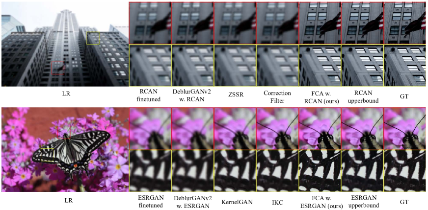
In this part, we compare our FCA with deblurring method (i.e., DeblurGANv2 (Kupyn et al. 2019)) and domain correction method (i.e., Correction Filter (Hussein, Tirer, and Giryes 2020)). Different from estimating internal degradation of image, these methods try to remove degradation from LR image and restore it to ideal state. We then classify these methods as ‘Correction SR’. As described in (Zhang, Zuo, and Zhang 2019), deblurring first works better than doing SR first. We then combine DeblurGANv2 with RCAN and ESRGAN, Correction Filter with RCAN respectively for comparison. Quantitative results in Table 1 show that these methods fail to reduce the domain gap. It is harder to recover the high-frequency components from the LR than degrading a clean one. Visual results in Figure 7 also confirms that FCA succeeds to recover realistic details with higher perceptual quality by accurate frequency adaptation.

Comparison with Blind SR

Among blind SR methods, KernelGAN (Bell-Kligler, Shocher, and Irani 2019) and IKC (Gu et al. 2019) are representative methods. KernelGAN estimates the specific degradation kernel for ZSSR (Shocher, Cohen, and Irani 2018) to generate SR results. For comparison, we run ZSSR with the bicubic kernel and put it under the type ‘Ideal SR’. IKC predicts the kernel and generates SR results in an iterative way. Quantitative and qualitative results are displayed in Table 1 and Figure 7. KernelGAN promotes the PSNR performance about $1.0$ compared with ZSSR. However, its degradation kernel estimation is not accurate, thus the SR process still suffers from frequency domain gap. Benefiting from correct guidance of the proposed FDC, our method achieves much better quality metric results than these representative blind methods. From the visual results, we can see that important low-frequency structures and realistic high-frequency details are reconstructed successfully.

Figure 8: Visual results with $\mathbf{4\times}$ compared with state-of-the-art SR methods on real images.

Ablation Study

Kernels	$\mathcal{L}_{WD}$	$\mathcal{L}_{FDC}$	$\mathcal{L}_{WD}\ \&\ \mathcal{L}_{FDC}$
ISO.1	27.07 / 0.7543 / 0.3688	27.59 / 0.7680 / 0.3448	27.35 / 0.7588 / 0.3629
ISO.3	23.23 / 0.6275 / 0.5361	25.45 / 0.6861 / 0.4647	25.50 / 0.6882 / 0.4589
ISO.[1,3]	23.98 / 0.6520 / 0.5199	24.63 / 0.6888 / 0.4446	24.84 / 0.6940 / 0.4500
ANI.	24.44 / 0.6590 / 0.5100	24.82 / 0.6850 / 0.4630	24.93 / 0.6870 / 0.4580

Table 2: Ablation study of the proposed frequency consistency loss and the adversarial loss. [PSNR/SSIM/LPIPS] results of three different models trained with different loss functions setting on $4\times$ synthetic images are listed. The best performances are marked in bold.

Furthermore, in order to analyze the effects of the proposed frequency consistency loss and the adversarial loss on the performance of the estimator, we conduct ablation experiments under the condition that only one loss is introduced into the generator on synthetic LR images. The results in Table 2 show that FDC plays a key role in the domain adaptation. Meanwhile, the final performance is improved from good cooperation with wavelet discriminator.

Experiments on Real World Images

Figure 9: Frequency density distributions of degraded LR and SR results by different methods on real-world images. The frequency distribution distance indicates that ESRGAN and KernelGAN generate inconsistent degraded images. Our FCA estimates proper kernels, thus obtaining LRs whose domain is closer to source domain.

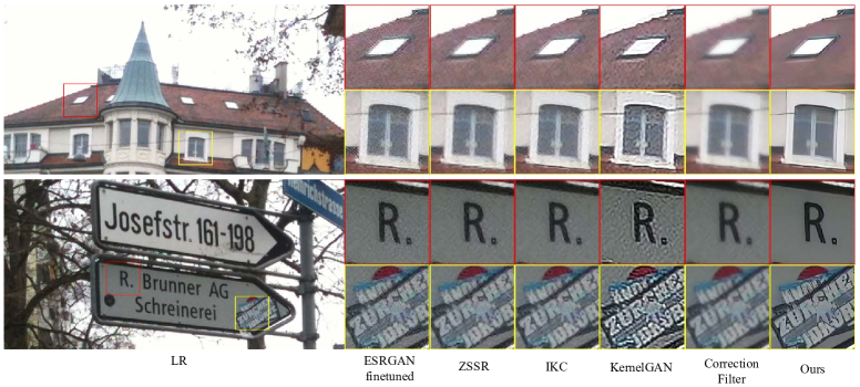
In the experiment on real-world dataset, we combine FCA with ESRGAN because its perception-oriented loss function helps to reconstruct richer details. For fair comparison, we finetune ESRGAN for the same iterations. Other comparative methods include ZSSR, KernelGAN, IKC, and Correction Filter. From the visual comparison in Figure 8, we notice that ESRGAN finetuned, ZSSR, IKC, Correction Filter generate over-smoothing results, while KernelGAN generates over-sharpening results. These blurry results that lacks of high-frequency details fail to enhance important edges (e.g., windows and letters). In contrast, our results show clear dividing line between two different surfaces. On the other hand, KernelGAN produces many undesirable artifacts though it looks good at first, which suggests its inaccurate estimation of degradation. We also provide no-reference assessment comparison results with the winning method (Impressionism (Ji et al. 2020)) in NTIRE 2020 Challenge on Real-World Image Super-Resolution (Lugmayr, Danelljan, and Timofte 2020). Our result is $14.5$ on PIQE (Venkatanath et al. 2015), $17.6\%$ lower than $17.6$ of Impressionism.

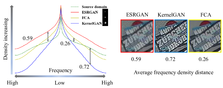
To provide quantitative measurement of frequency density distance, we propose to calculate it as follows:

$$\bar{\mathcal{D}}(X,Y) =\frac{1}{n}\Sigma_{l}[|\mathcal{F}_{X}(l)-\mathcal{F}_{Y}(l)|],$$ (13)

where $\bar{\mathcal{D}}(X,Y)$ denotes the distance between domain $X$ and $Y$, $n$ is the number of frequency. By FCA’s accurate estimation, the degraded LRs are close to source domain as shown in Figure 9, thus obtaining more natural result.

Conclusion

In this paper, we propose a novel frequency consistent adaptation for real-world super-resolution, which keeps the degraded images and the original ones consistent in the frequency domain. In the proposed FCA, we carefully design a frequency domain density comparator to estimate the degradation of the source domain through an unsupervised training method. Experiments on synthetic and real-world datasets show that the proposed FCA is effective in real-world SR, avoiding performance dropped caused by incorrect degradation. As a general unsupervised degradation estimation method, FCA can be combined with easy-implemented SR models and achieves state-of-the-art performance on real images. Experiments show our SR results achieve higher fidelity and better visual perception.

References

- Bell-Kligler, Shocher, and Irani (2019) Bell-Kligler, S.; Shocher, A.; and Irani, M. 2019. Blind Super-Resolution Kernel Estimation Using an Internal-GAN. In Advances in Neural Information Processing Systems (NeurIPS), 284–293.
- Bengio (2013) Bengio, Y. 2013. Deep Learning of Representations: Looking Forward. In International Conference on Statistical Language and Speech Processing, 1–37. Springer.
- Chen et al. (2018) Chen, Y.; Tai, Y.; Liu, X.; Shen, C.; and Yang, J. 2018. FSRNet: End-to-End Learning Face Super-Resolution with Facial Priors. In Proceedings of the IEEE Conference on Computer Vision and Pattern Recognition (CVPR), 2492–2501.
- Dong et al. (2015) Dong, C.; Loy, C. C.; He, K.; and Tang, X. 2015. Image Super-Resolution Using Deep Convolutional Networks. IEEE Transactions on Pattern Analysis and Machine Intelligence (TPAMI) 38(2): 295–307.
- Freeman, Jones, and Pasztor (2002) Freeman, W. T.; Jones, T. R.; and Pasztor, E. C. 2002. Example-based Super-Resolution. IEEE Computer Graphics and Applications 22(2): 56–65.
- Fritsche, Gu, and Timofte (2019) Fritsche, M.; Gu, S.; and Timofte, R. 2019. Frequency Separation for Real-World Super-Resolution. arXiv preprint arXiv:1911.07850 .
- Glasner, Bagon, and Irani (2009) Glasner, D.; Bagon, S.; and Irani, M. 2009. Super-Resolution From a Single Image. In Proceedings of the 12th International Conference on Computer Vision (ICCV), 349–356. IEEE.
- Goodfellow et al. (2014) Goodfellow, I.; Pouget-Abadie, J.; Mirza, M.; Xu, B.; Warde-Farley, D.; Ozair, S.; Courville, A.; and Bengio, Y. 2014. Generative Adversarial Nets. In Advances in Neural Information Processing Systems (NeurIPS), 2672–2680.
- Gu et al. (2019) Gu, J.; Lu, H.; Zuo, W.; and Dong, C. 2019. Blind Super-Resolution with Iterative Kernel Correction. In Proceedings of the IEEE Conference on Computer Vision and Pattern Recognition (CVPR), 1604–1613.
- Haris, Shakhnarovich, and Ukita (2018) Haris, M.; Shakhnarovich, G.; and Ukita, N. 2018. Deep Back-Projection Networks for Super-Resolution. In Proceedings of the IEEE Conference on Computer Vision and Pattern Recognition (CVPR), 1664–1673.
- He et al. (2019) He, X.; Mo, Z.; Wang, P.; Liu, Y.; Yang, M.; and Cheng, J. 2019. Ode-Inspired Network Design for Single Image Super-Resolution. In Proceedings of the IEEE Conference on Computer Vision and Pattern Recognition (CVPR), 1732–1741.
- Hu et al. (2019) Hu, X.; Mu, H.; Zhang, X.; Wang, Z.; Tan, T.; and Sun, J. 2019. Meta-SR: A Magnification-Arbitrary Network for Super-Resolution. In Proceedings of the IEEE Conference on Computer Vision and Pattern Recognition (CVPR), 1575–1584.
- Hussein, Tirer, and Giryes (2020) Hussein, S. A.; Tirer, T.; and Giryes, R. 2020. Correction Filter for Single Image Super-Resolution: Robustifying Off-the-Shelf Deep Super-Resolvers. In Proceedings of the IEEE/CVF Conference on Computer Vision and Pattern Recognition (CVPR), 1428–1437.
- Ignatov et al. (2017) Ignatov, A.; Kobyshev, N.; Timofte, R.; Vanhoey, K.; and Van Gool, L. 2017. DSLR-Quality Photos on Mobile Devices with Deep Convolutional Networks. In Proceedings of the IEEE International Conference on Computer Vision (ICCV), 3277–3285.
- Ji et al. (2020) Ji, X.; Cao, Y.; Tai, Y.; Wang, C.; Li, J.; and Huang, F. 2020. Real-World Super-Resolution via Kernel Estimation and Noise Injection. In Proceedings of the IEEE/CVF Conference on Computer Vision and Pattern Recognition (CVPR) Workshops, 466–467.
- Johnson, Alahi, and Fei-Fei (2016) Johnson, J.; Alahi, A.; and Fei-Fei, L. 2016. Perceptual Losses for Real-Time Style Transfer and Super-Resolution. In Proceedings of the European Conference on Computer Vision (ECCV), 694–711. Springer.
- Kim, Kwon Lee, and Mu Lee (2016) Kim, J.; Kwon Lee, J.; and Mu Lee, K. 2016. Accurate Image Super-Resolution Using Very Deep Convolutional Networks. In Proceedings of the IEEE Conference on Computer Vision and Pattern Recognition (CVPR), 1646–1654.
- Kupyn et al. (2019) Kupyn, O.; Martyniuk, T.; Wu, J.; and Wang, Z. 2019. Deblurgan-v2: Deblurring (Orders-of-Magnitude) Faster and Better. In Proceedings of the IEEE International Conference on Computer Vision (ICCV), 8878–8887.
- Lai et al. (2017) Lai, W.-S.; Huang, J.-B.; Ahuja, N.; and Yang, M.-H. 2017. Deep Laplacian Pyramid Networks for Fast and Accurate Super-Resolution. In Proceedings of the IEEE Conference on Computer Vision and Pattern Recognition (CVPR), 624–632.
- Ledig et al. (2017) Ledig, C.; Theis, L.; Huszár, F.; Caballero, J.; Cunningham, A.; Acosta, A.; Aitken, A.; Tejani, A.; Totz, J.; Wang, Z.; et al. 2017. Photo-Realistic Single Image Super-Resolution Using a Generative Adversarial Network. In Proceedings of the IEEE Conference on Computer Vision and Pattern Recognition (CVPR), 4681–4690.
- Li et al. (2019) Li, Z.; Yang, J.; Liu, Z.; Yang, X.; Jeon, G.; and Wu, W. 2019. Feedback Network for Image Super-Resolution. In Proceedings of the IEEE Conference on Computer Vision and Pattern Recognition (CVPR), 3867–3876.
- Lim et al. (2017) Lim, B.; Son, S.; Kim, H.; Nah, S.; and Mu Lee, K. 2017. Enhanced Deep Residual Networks for Single Image Super-Resolution. In Proceedings of the IEEE conference on Computer Vision and Pattern Recognition (CVPR) Workshops, 136–144.
- Lugmayr, Danelljan, and Timofte (2020) Lugmayr, A.; Danelljan, M.; and Timofte, R. 2020. NTIRE 2020 Challenge on Real-World Image Super-Resolution: Methods and Results. In Proceedings of the IEEE/CVF Conference on Computer Vision and Pattern Recognition (CVPR) Workshops, 494–495.
- Mao et al. (2017) Mao, X.; Li, Q.; Xie, H.; Lau, R. Y.; Wang, Z.; and Paul Smolley, S. 2017. Least Squares Generative Adversarial Networks. In Proceedings of the IEEE international Conference on Computer Vision (ICCV), 2794–2802.
- Pan et al. (2018) Pan, J.; Liu, S.; Sun, D.; Zhang, J.; Liu, Y.; Ren, J.; Li, Z.; Tang, J.; Lu, H.; Tai, Y.-W.; et al. 2018. Learning Dual Convolutional Neural Networks for Low-Level Vision. In Proceedings of the IEEE Conference on Computer Vision and Pattern Recognition (CVPR), 3070–3079.
- Qiu et al. (2019) Qiu, Y.; Wang, R.; Tao, D.; and Cheng, J. 2019. Embedded Block Residual Network: A Recursive Restoration Model for Single-Image Super-Resolution. In Proceedings of the IEEE International Conference on Computer Vision (CVPR), 4180–4189.
- Shocher, Cohen, and Irani (2018) Shocher, A.; Cohen, N.; and Irani, M. 2018. “Zero-Shot” Super-Resolution Using Deep Internal Learning. In Proceedings of the IEEE Conference on Computer Vision and Pattern Recognition (CVPR), 3118–3126.
- Soh et al. (2019) Soh, J. W.; Park, G. Y.; Jo, J.; and Cho, N. I. 2019. Natural and Realistic Single Image Super-Resolution with Explicit Natural Manifold Discrimination. In Proceedings of the IEEE Conference on Computer Vision and Pattern Recognition (CVPR), 8122–8131.
- Tai, Yang, and Liu (2017) Tai, Y.; Yang, J.; and Liu, X. 2017. Image Super-Resolution via Deep Recursive Residual Network. In Proceedings of the IEEE Conference on Computer Vision and Pattern Recognition (CVPR), 3147–3155.
- Tai et al. (2017) Tai, Y.; Yang, J.; Liu, X.; and Xu, C. 2017. Memnet: A Persistent Memory Network for Image Restoration. In Proceedings of the IEEE International Conference on Computer Vision (ICCV), 4539–4547.
- Timofte et al. (2017) Timofte, R.; Agustsson, E.; Van Gool, L.; Yang, M.-H.; and Zhang, L. 2017. NTIRE 2017 Challenge on Single Image Super-Resolution: Methods and Results. In Proceedings of the IEEE Conference on Computer Vision and Pattern Recognition (CVPR) Workshops, 114–125.
- Venkatanath et al. (2015) Venkatanath, N.; Praneeth, D.; Bh, M. C.; Channappayya, S. S.; and Medasani, S. S. 2015. Blind Image Quality Evaluation Using Perception Based Features. In 2015 Twenty First National Conference on Communications (NCC), 1–6. IEEE.
- Wang et al. (2018a) Wang, X.; Yu, K.; Dong, C.; and Change Loy, C. 2018a. Recovering Realistic Texture in Image Super-Resolution by Deep Spatial Feature Transform. In Proceedings of the IEEE Conference on Computer Vision and Pattern Recognition (CVPR), 606–615.
- Wang et al. (2018b) Wang, X.; Yu, K.; Wu, S.; Gu, J.; Liu, Y.; Dong, C.; Qiao, Y.; and Change Loy, C. 2018b. ESRGAN: Enhanced Super-Resolution Generative Adversarial Networks. In Proceedings of the European Conference on Computer Vision (ECCV).
- Wei et al. (2020) Wei, Y.; Gu, S.; Li, Y.; and Jin, L. 2020. Unsupervised Real-World Image Super Resolution via Domain-Distance Aware Training. arXiv preprint arXiv:2004.01178 .
- Yin et al. (2019) Yin, X.; Tai, Y.; Huang, Y.; and Liu, X. 2019. FAN: Feature Adaptation Network for Surveillance Face Recognition and Normalization. arXiv:1911.11680v1 .
- Zhang, Zuo, and Zhang (2018) Zhang, K.; Zuo, W.; and Zhang, L. 2018. Learning a Single Convolutional Super-Resolution Network for Multiple Degradations. In Proceedings of the IEEE Conference on Computer Vision and Pattern Recognition (CVPR), 3262–3271.
- Zhang, Zuo, and Zhang (2019) Zhang, K.; Zuo, W.; and Zhang, L. 2019. Deep Plug-and-Play Super-Resolution for Arbitrary Blur Kernels. In Proceedings of the IEEE Conference on Computer Vision and Pattern Recognition (CVPR), 1671–1681.
- Zhang et al. (2018a) Zhang, R.; Isola, P.; Efros, A. A.; Shechtman, E.; and Wang, O. 2018a. The Unreasonable Effectiveness of Deep Features as a Perceptual Metric. In Proceedings of the IEEE Conference on Computer Vision and Pattern Recognition (CVPR), 586–595.
- Zhang et al. (2019a) Zhang, W.; Liu, Y.; Dong, C.; and Qiao, Y. 2019a. RankSRGAN: Generative Adversarial Networks with Ranker for Image Super-Resolution. In Proceedings of the IEEE International Conference on Computer Vision (ICCV), 3096–3105.
- Zhang et al. (2018b) Zhang, Y.; Li, K.; Li, K.; Wang, L.; Zhong, B.; and Fu, Y. 2018b. Image Super-Resolution Using Very Deep Residual Channel Attention Networks. In Proceedings of the European Conference on Computer Vision (ECCV), 286–301.
- Zhang et al. (2019b) Zhang, Z.; Wang, Z.; Lin, Z.; and Qi, H. 2019b. Image Super-Resolution By Neural Texture Transfer. In Proceedings of the IEEE Conference on Computer Vision and Pattern Recognition (CVPR), 7982–7991.
- Zheng et al. (2018) Zheng, H.; Ji, M.; Wang, H.; Liu, Y.; and Fang, L. 2018. CrossNet: An End-to-End Reference-based Super Resolution Network Using Cross-Scale Warping. In Proceedings of the European Conference on Computer Vision (ECCV), 88–104.
- Zhou and Susstrunk (2019) Zhou, R.; and Susstrunk, S. 2019. Kernel Modeling Super-Resolution on Real Low-Resolution Images. In Proceedings of the IEEE International Conference on Computer Vision (ICCV), 2433–2443.