The updated BaSTI stellar evolution models and isochrones: II. $\alpha-$enhanced calculations

Abstract

This is the second paper of a series devoted to present an updated release of the BaSTI (a Bag of Stellar Tracks and Isochrones) stellar model and isochrone library. Following the publication of the updated solar scaled library, here we present the library for a $\alpha-$enhanced heavy element distribution. These new $\alpha-$enhanced models account for all improvements and updates in the reference solar metal distribution and physics inputs, as in the new solar scaled library. The models cover a mass range between 0.1 and $15~{}M_{\odot}$, 18 metallicities between [Fe/H]=$-$3.20 and $+$0.06 with $[\alpha/Fe]=+0.4$ , and a helium to metal enrichment ratio $\Delta{Y}$/$\Delta{Z}$=1.31. For each metallicity, He-enhanced stellar models are also provided. The isochrones cover (typically) an age range between 20 Myr and 14.5 Gyr, including consistently the pre-main sequence phase. Asteroseismic properties of the theoretical models have also been calculated. Models and isochrones have been compared with results from independent calculations, with the previous BaSTI release, and also with selected observations, to test the accuracy/reliability of these new calculations. All stellar evolution tracks, asteroseismic properties and isochrones are made publicly available at http://basti-iac.oa-teramo.inaf.it

1 Introduction

Accurate sets of stellar model calculations and isochrones are necessary to interpret a vast array of spectroscopic and photometric observations of individual stars, star clusters, and galaxies, both resolved and unresolved.

Between 2004 and 2013 we have built and made publicly available the BaSTI (a Bag of Stellar Tracks and Isochrones) stellar models and isochrones library (Pietrinferni et al., 2004, 2006; Cordier et al., 2007; Pietrinferni et al., 2009; Salaris et al., 2010; Pietrinferni et al., 2013), which has been extensively employed by the astronomical community. This library covers a wide range of masses, evolutionary phases, chemical compositions, and also provides integrated magnitudes and spectra of single-age, single-metallicity populations.

In the intervening years, improvements in the physics and chemical inputs of stellar model calculations have become available, most notably the revision of the solar metal composition (e.g., Bergemann & Serenelli, 2014, and references therein), plus new electron conduction opacities and some improved reaction rates. We have therefore embarked in an update of the BaSTI library, starting with models and isochrones for solar scaled chemical compositions, presented in Hidalgo et al. (2018). In this new BaSTI release we have extended the mass range both towards lower and higher masses, and we also provide some basic asteroseismic properties of the models.

This second paper presents the new BaSTI release of models and isochrones for a $\alpha-$enhanced metal distribution, suitable to study populations in galactic haloes, spheroids and dwarf galaxies. Our calculations are the latest addition to the list of $\alpha-$enhanced model sets computed over the last 22 years by various authors, sometimes restricted to the mass and metallicity range of Galactic halo stars (Salaris & Weiss, 1998; VandenBerg et al., 2000; Salasnich et al., 2000; Kim et al., 2002; Dotter et al., 2008a; VandenBerg et al., 2012; Fu et al., 2018).

The plan of the paper is as follows. Section 2 briefly summarises the physics inputs adopted in the new computations, and the heavy element distribution. Section 3 presents the stellar model grid, including the mass and chemical composition parameter space. Section 4 shows comparisons between these new models and previous calculations available in the literature, whilst Sect. 5 compares the models with selected observational benchmarks. Final remarks follow in Sect. 6.

2 Stellar evolution code, metal distribution and physics inputs

We have employed the same stellar evolution code as in Hidalgo et al. (2018) –hereafter Paper I– and the reader is referred to that paper for more information about the technical improvements since the first release of the BaSTI database.

The adopted $\alpha$-enhanced heavy element distribution is listed in Table 1: The $\alpha$-elements O, Ne, Mg, Si, S, Ca, and Ti have been uniformly enhanced with respect to Fe by [$\alpha$/Fe]$=+0.4$, compared to the Caffau et al. (2011) solar metal distribution employed in Paper I. A uniform enhancement of all these $\alpha$-elements has been adopted also in other large stellar model grids (see, e.g., Kim et al., 2002; Dotter et al., 2008a; VandenBerg et al., 2014) and is generally consistent with results from spectroscopy (see, e.g., Cayrel de Strobel et al., 1997; Hayes et al., 2018; Mashonkina et al., 2019; Ramírez et al., 2012). Just oxygen might be slightly more enhanced than the other $\alpha$-elements, by approximately an extra 0.1-0.15 dex. An extra enhancement of oxygen makes isochrones of a given age and [Fe/H] slightly fainter and cooler in the main sequence turn-off region. This effect is mimicked by considering a slightly older age for isochrones without the extra oxygen, at the level of at most just 3-4% percent if [O/Fe] is increased by 0.1-0.15 dex (see Dotter et al., 2007; VandenBerg et al., 2012). Also, the $T_{\mathrm{e}ff}$ of the lower main sequence in the regime of very low-mass stars would become slightly cooler, at the level of about just 2% (see Dotter et al., 2007).

The value [$\alpha$/Fe]$=+0.4$ adopted in our calculations is close to the upper limits measured in the Galaxy; an interpolation in [$\alpha$/Fe] between our solar scaled models and these new ones can provide accurate evolutionary tracks and isochrones for any intermediate $\alpha$-enhancement, as verified with the DSEP model library, that includes several different values of [$\alpha$/Fe] between $-$0.2 and +0.8 (Dotter et al., 2008a).

Our adopted $\alpha$-enhanced distribution has been used consistently in the nuclear reaction network, in the calculation of radiative and electron conduction opacities, as well as in the equation of state (EOS). The sources for opacities and EOS are the same as described in Paper I.

Table 1: The adopted $\alpha-$enhanced heavy element distribution.

Element	Number fraction	Mass fraction
C	0.132021	0.089896
N	0.030250	0.024020
O	0.603476	0.547368
Ne	0.123221	0.140962
Na	0.000850	0.001108
Mg	0.038070	0.052456
Al	0.001260	0.001927
Si	0.037210	0.059246
P	0.000120	0.000211
S	0.014810	0.026918
Cl	0.000070	0.000141
Ar	0.001380	0.003125
K	0.000050	0.000111
Ca	0.002240	0.005090
Ti	0.000090	0.000244
Cr	0.000200	0.000590
Mn	0.000130	0.000405
Fe	0.013830	0.043787
Ni	0.000720	0.002396

The nuclear reaction and neutrino energy loss rates, treatment of superadiabatic convection (all calculations employ a mixing length ${\rm\alpha_{ML}=2.006}$ obtained from a solar model calibration), outer boundary conditions, treatment of overshooting from the convective cores and atomic diffusion (without radiative levitation), are all as described in detail in Paper I.

Regarding the outer boundary conditions, for models with masses ${\rm M\leq 0.45M_{\odot}}$ we use outer boundary conditions provided by the PHOENIX non-gray model atmospheres (see, Hidalgo et al., 2018, and references therein) described in Allard et al. (2012). More precisely, we employ the so-called BT-Settl model set.

As in Paper I, mass loss is included with the Reimers (1975) formula, and the free parameter $\eta$ is set to 0.3, following the asteroseismic constraints discussed in Miglio et al. (2012). We continue to use the Reimers (1975) formula because its free parameter has been calibrated through asteroseismology in nearby open clusters, and also to be homogeneous with our solar scaled calculations. Prompted by our referee, we have calculated test models with masses equal to 0.8, 1.8 and 4$M_{\odot}$ at a representative [Fe/H]=$-$1.2, employing the more modern (Schröder & Cuntz, 2005) mass loss formula. We have implemented equation 4 in (Schröder & Cuntz, 2005) with the free parameter $\eta_{SC}$ set to $8\times 10^{-14}~{}M_{\odot}~{}yr^{-1}$ as recommended by the authors, multiplied by another free parameter $\eta_{1}$, as done in Valcarce et al. (2012). We have then determined the value of $\eta_{1}$ that provides the best agreement with our calculations based on the Reimers formula. We found that for the 0.8 and 1.8 $M_{\odot}$ models a value $\eta_{1}$=0.6 matches our Reimers calculations in terms of both HRD tracks and amount of mass lost. For the 4$M_{\odot}$ a value $\eta_{1}$=0.3 gives the best match.

For the 10 and 15$M_{\odot}$ models we have experimented using the Nieuwenhuijzen & de Jager (1990) mass loss formula instead of the Reimers one. Main sequence HRD and lifetimes are identical for both masses and both mass loss choices, despite the fact that models calculated with the Nieuwenhuijzen & de Jager (1990) formula lose 0.1 and 0.3$M_{\odot}$ respectively, against 0.01 and 0.02$M_{\odot}$ for the reference Reimers calculations. The HRD and lifetimes of the following evolution are also barely affected by the choice of the mass loss, even though by the end of core He-burning the calculations with Nieuwenhuijzen & de Jager (1990) formula have lost 0.32 and 0.62$M_{\odot}$ respectively, against 0.03$M_{\odot}$ for both Reimers computations.

Table 2: Initial values of the heavy element mass fraction $Z$, helium mass fraction $Y$, the corresponding [Fe/H] and [M/H], and the additional (enhanced) values of $Y$ at fixed $Z$, of our model grid.

Z	Y	[Fe/H]	[M/H]	${\rm Y_{enh,1}}$	${\rm Y_{enh,2}}$
0.0000199	0.247013	$-3.20$	$-2.90$	0.275	0.30
0.0000996	0.247117	$-2.50$	$-2.20$	0.275	0.30
0.0001988	0.247247	$-2.20$	$-1.90$	0.275	0.30
0.0003974	0.247506	$-1.90$	$-1.60$	0.275	0.30
0.0006275	0.247807	$-1.70$	$-1.40$	0.275	0.30
0.0008860	0.248146	$-1.55$	$-1.25$	0.275	0.30
0.0012500	0.248620	$-1.40$	$-1.10$	0.275	0.30
0.0015720	0.249040	$-1.30$	$-1.00$	0.275	0.30
0.0019750	0.249569	$-1.20$	$-0.90$	0.275	0.30
0.0027850	0.250628	$-1.05$	$-0.75$	0.275	0.30
0.0039200	0.252112	$-0.90$	$-0.60$	0.275	0.30
0.0061700	0.255054	$-0.70$	$-0.40$	0.275	0.30
0.0077300	0.257100	$-0.60$	$-0.30$	0.275	0.30
0.0120800	0.262790	$-0.40$	$-0.10$	$\cdots$	0.30
0.0150700	0.266905	$-0.30$	0.00	$\cdots$	0.30
0.0187500	0.271502	$-0.20$	0.10	$\cdots$	0.30
0.0242700	0.278717	$-0.08$	0.22	$\cdots$	0.30
0.0325800	0.289584	0.06	0.36	$\cdots$	0.32

3 The $\alpha$-enhanced model library

This new BaSTI $\alpha$-enhanced model library includes calculations for 18 values of the initial metallicity –a larger number than in the previous BaSTI release (Pietrinferni et al., 2006)– ranging from ${\rm Z\approx 2\times 10^{-5}}$ (${\rm[Fe/H]=-3.20}$) to ${\rm Z\approx 0.033}$ (${\rm[Fe/H]=+0.06}$). The initial values of $Y$ at a given $Z$ have been fixed assuming a primordial $Y$=0.247 and a helium-enrichment ratio $\Delta{Y}/\Delta{Z}=1.31$, as discussed in Paper I.

This $\alpha$-enhanced grid has been calculated for the same [Fe/H] values of the solar scaled one of Paper I, therefore at a given [Fe/H] the values of $Z$ are higher than for the solar scaled grid, because of the different metal mixture.

An important difference with respect to the solar scaled grid of Paper I is that this new $\alpha-$enhanced release includes multiple values of the initial He abundance, at a given $Z$. The complete list of available chemical compositions is given in Table 2.

The purpose of these calculations with several initial He abundances is to study stellar populations in environments hosting He-rich stars, such as the Galactic bulge, elliptical galaxies, and also globular clusters. In the case of individual globular clusters, He-enhanced stellar populations display specific patterns of variations of C, N, O, Na, Mg and Al with respect to the standard $\alpha$-enhanced composition of the helium normal component (see, e.g. Bastian & Lardo, 2018; Gratton et al., 2019; Cassisi & Salaris, 2020, for recent reviews). As long as the sum C+N+O is unchanged by these abundance patterns (which seems to be the case for most of the clusters) $\alpha$-enhanced calculations are appropriate to study globular clusters’ multiple populations in the HRD, in optical and generally in infrared colour-magnitude-diagrams (CMDs) (see, e.g. Salaris et al., 2006; Pietrinferni et al., 2009; Cassisi & Salaris, 2020, and references therein). For CMDs involving wavelengths shorter than the optical range, and for the very low-mass stars in the infrared, appropriate bolometric corrections that account for the specific metal abundance patterns need to be calculated and applied to our isochrones (see Cassisi & Salaris, 2020).

For each composition – but for the He-enhanced ones (see below) – we have computed 56 evolutionary sequences, in the mass range between $0.1~{}M_{\odot}$ and $15~{}M_{\odot}$). For initial masses below $0.2~{}M_{\odot}$ we computed evolutionary tracks for masses equal to 0.10, 0.12, 0.15 and $0.18~{}M_{\odot}$. In the range between 0.2 and $0.7~{}M_{\odot}$ we employed a mass step equal to $0.05~{}M_{\odot}$. Mass steps equal to $0.1~{}M_{\odot}$, $0.2~{}M_{\odot}$, 0.5 $M_{\odot}$ and 1 $M_{\odot}$ have been adopted for the mass ranges $0.7-2.6~{}M_{\odot}$, $2.6-3.0~{}M_{\odot}$, $3.0-10.0~{}M_{\odot}$, and masses larger than $10.0M_{\odot}$, respectively. For the He-enhanced chemical compositions, the upper mass limit was set to $2.0M_{\odot}$, to cover the observed age range of the massive clusters that display multiple stellar populations, which has a lower limit around $\sim 1.2-1.4$ Gyr (see, e.g. Cabrera-Ziri et al., 2020, and references therein) .

All models less massive than $4.0~{}M_{\odot}$ have been computed from the pre-main sequence (pre-MS), whereas more massive model calculations started from the zero age MS. Relevant to the pre-MS calculations, the initial mass fractions of D, ${\rm{}^{3}He}$ and ${\rm{}^{7}Li}$ are set to $3.9\times 10^{-5}$, $2.3\times 10^{-5}$, and $2.6\times 10^{-9}$ respectively (see Paper I).

As in Paper I, all evolutionary models –but the very low-mass ones whose core H-burning lifetime is much longer than the Hubble time– have been calculated until the start of the thermal pulses on the asymptotic giant branch, or C-ignition for the more massive ones. In case of the long-lived lower mass models, we have stopped the calculations when the central H mass fraction is $\sim$0.3 (corresponding to ages already much larger than the Hubble time).

For each initial chemical composition we provide also an extended set of core He-burning models suited to study the horizontal branch (HB) in old stellar populations. For each pair ($Z$, $Y$) we have computed models of varying total mass (with small mass steps) and fixed He-core mass. Both He-core mass and chemical abundances in the envelope of the HB models are taken from the model of a red giant branch (RGB) progenitor at the He-flash, with an age of $\sim 12.5$ Gyr.

Prompted by the referee and the results by Valcarce et al. (2012), we have quantified the effect of changing the age of the RGB progenitors by performing numerical experiments at [Fe/H]=$-$1.2. A decrease of the progenitor age from the reference 12.5 Gyr to 6 Gyr lowers the He-core mass at helium ignition by 0.004$M_{\odot}$ (from 0.4865$M_{\odot}$ to 0.4822$M_{\odot}$) but increases the helium abundance in the envelope by $\Delta Y$=0.01 (from $Y$=0.26 to $Y$=0.27) due to the variation of the efficiency of the first dredge-up. As a consequence, the luminosity of the zero age HB (ZAHB) is roughly unchanged, and all tracks for masses above 0.5$M_{\odot}$ are essentially identical to the case of 12.5 Gyr progenitors. Only HB models with mass below this threshold –unlikely to be found in 6 Gyr old stellar populations– are affected by this large change of the progenitor age. These tracks are increasingly shifted to lower $T_{\mathrm{e}ff}$ with decreasing mass, by up to 15% for the lowest HB mass (equal to 0.487$M_{\odot}$, with a ZAHB effective temperature of 30,000 K for the model with a 12.5 Gyr progenitor) but their ZAHB luminosity is unchanged.

When the age changes from 12.5 to 10 Gyr the variations of the He-core mass and surface helium abundance are about half these values, whilst an increase of the age from 12.5 to 14 Gyr leaves core masses and helium abundances unaffected.

We have also performed a second test along the following lines. Our HB models are computed considering He-core mass and envelope composition of a progenitor whose evolution is calculated with our reference choice of mass loss efficiency –Reimers formula with $\eta$=0.3. This means that, for example, a HB model with total mass equal to 0.5$M_{\odot}$ has been computed with core mass and envelope composition of a progenitor that at He ignition had a mass larger than this value. To check whether this procedure introduces any systematics in our HB calculations, we have computed the evolution of several 0.8$M_{\odot}$ RGB progenitor models at [Fe/H]=$-$1.2 (with an age at the tip of the RGB equal to about 12.5 Gyr) varying $\eta$ from 0 to 0.63, to reach masses between 0.8 and 0.487$M_{\odot}$ at the He-flash. We have then calculated the HB evolution of these masses, to compare with the corresponding results obtained with our reference method to calculate HB models. Also in this case, only HB models with mass below 0.5$M_{\odot}$ –with very thin envelopes and inefficient H-burning shell– are affected. In this mass range the He-core mass has decreased by 0.001$M_{\odot}$ compared to calculations for $\eta$=0.3, and the tracks are shifted to temperatures lower by at most 7% for the lowest mass. The ZAHB luminosities are unchanged.

As for all evolutionary sequences available in the BaSTI library, also these new tracks have been ‘normalized’to the same number of points to calculate isochrones, and more in general for ease of interpolation and implementation in stellar population synthesis tools. As extensively discussed in Pietrinferni et al. (2004) and Paper I, this normalization is based on the identification of some characteristic homologous points (key points) corresponding to well-defined evolutionary stages along each track. The choice of the key points, and the number of points distributed between two consecutive key points are as described in Paper I. For each chemical composition, these normalized evolutionary tracks are used to compute extended sets of isochrones for ages between 20 Myr and 14.5 Gyr (older isochrones can be computed upon request from the authors). For the He-enhanced compositions the isochrone age range is between $\sim 600$ Myr and 14.5 Gyr.

The solar scaled calculations of Paper I included four model grids, computed with different choices regarding whether convective core overshooting, atomic diffusion and mass loss are included or neglected in the calculations (see Table 3 in Paper I). For these $\alpha$-enhanced calculations we provide just one grid, corresponding to what we consider to be a best physics scenario, that corresponds to Case a of Table 3 in Paper I. This means that these models all include convective core overshooting, atomic diffusion and mass loss.

Bolometric luminosities and effective temperatures along evolutionary tracks and isochrones have been translated to magnitudes and colours using sets of bolometric corrections (BCs) calculated as described in Paper I. More specifically, we calculated BCs with the ATLAS 9 suite of programs (Kurucz, 1970), for the same $\alpha$-enhanced metal distribution of the stellar evolution models. As in Paper I, these BCs have been complemented in the low $T_{\mathrm{e}ff}$ and high-gravity regime with the spectral library by Husser et al. (2013) for [$\alpha$/Fe]=0.4, calculated with the PHOENIX code (Hauschildt & Baron, 1999).

Table 3 lists all photometric systems presently available in the library, and provides all the relevant information about the source for the response curve of each filter, and the zero-points calibration.

Table 3: The photometric systems presently available in the library.

Photometric system	Calibration	Passbands	Zero-points
2MASS	Vegamag	Cohen et al. (2003)	Cohen et al. (2003)
DECam	ABmag	CTIO	0
Euclid (VIS $+$ NISP)	ABmag	Euclid mission database	0
Gaia DR1	Vegamag	Jordi et al. (2010)	Jordi et al. (2010)
Gaia DR2	Vegamag	Maíz Apellániz & Weiler (2018)(MAW)	MAW
Gaia DR3	Vegamag	Gaia Collaboration et al. (2020)	Gaia Collaboration et al. (2020)
GALEX	ABmag	NASA	0
Hipparcos + Tycho	ABmag	Bessell & Murphy (2012)	Bessell & Murphy (2012)
HST (WFPC2)	Vegamag	SYNPHOT	SYNPHOT
HST ( WFC3)	Vegamag	HST User Documentation	WFC3 webpage
HST (ACS)	Vegamag	HST User Documentation	ACS webpage
J-PLUS	ABmag	J-PLUS collab.	0
JWST (NIRCam)	Vegamag	JWST User Documentation	SYNPHOT
JWST (NIRISS)	Vegamag	JWST User Documentation	SYNPHOT
Kepler	ABmag	Kepler collab.	0
PanSTARSS1	ABmag	Tonry et al. (2012)	0
SAGE	ABmag	SAGE collab.	0
Skymapper	ABmag	Bessell (2011)	0
Sloan	ABmag	Doi et al. (2010)	Dotter et al. (2008b)
Spitzer (IRAC)	Vegamag	NASA	Groenewegen (2006)
Strömgren	Vegamag	Maíz Apellániz (2006)	Maíz Apellániz (2006)
Subaru (HSC)	ABmag	HSC collab.	0
SWIFT (UVOT)	Vegamag	NASA	Poole et al. (2008)
TESS	ABmag	NASA	0
UBVRIJHKLM	Vegamag	Bessell & Brett (1988); Bessell (1990)	Bessell et al. (1998)
UVIT (FUV+NUV+VIS)	ABmag	UVIT collab.	Tandon et al. (2017)
Vera C. Rubin Obs.	ABmag	LSST collaboration	0
VISTA	Vegamag	ESO	Rubele et al. (2012)
WFIRST (WFI)	Vegamag	WFIRST reference information	SYNPHOT
WISE	Vegamag	WISE collab.	Wright et al. (2010)

Finally, adiabatic oscillation frequencies for p-modes for all models have been computed by using the Aarhus adiabatic oscillation package (Christensen-Dalsgaard, 2008) as described in Paper I. We do not calculate g-mode frequencies because they have limited applications due to the mode identification issue, and the computation is expensive. We provide radial, dipole, quadrupole, and octupole p-mode frequencies for the models with central hydrogen mass fraction larger than $10^{-4}$, and only the radial mode frequencies for more evolved models. We note that non-radial modes can have mixed character in evolved models, i.e. they behave like p- and g-modes depending on the depth. Although mixed modes have been observed in subgiant branch and RGB stars, their analysis as well as the comparison with stellar models are still challenging. We have also calculated the frequency of maximum power ($\nu_{\rm max}$), the large frequency separation for the radial mode frequencies ($\Delta\nu_{0}$), and the asymptotic period spacing for the dipole mode frequencies ($\Delta P_{1}$).

3.1 A note on atomic diffusion

All currently available public stellar model libraries that include atomic diffusion (as our new calculations), do account for the effect of pressure gradients (gravitational settling), temperature and chemical gradients, but neglect radiative levitation. As shown by Turcotte et al. (1998), radiative levitation does not have any major impact on the solar model, on the solar calibration of the mixing length and the initial helium abundance of the Sun (see their Table  6), but it is expected to have a more relevant effect on models with less massive convective envelopes, like low-mass metal poor models around the main sequence turn off (see Richard et al., 2002). To this purpose, Fig. 7 of Richard et al. (2002) compares selected evolutionary properties of models with 0.8$M_{\odot}$, and initial [Fe/H]=$-$2.31, with and without the inclusion of radiative levitation. This comparison shows that the evolutionary track with radiative levitation is almost identical to the one calculated with atomic diffusion without levitation. There is just a small difference in $T_{\mathrm{e}ff}$ around the main sequence turn off, the track with levitation being cooler by less than 50 K: Luminosities and evolutionary timescales are identical. The major difference is the surface abundance of Fe, that is enhanced compared to the initial value in the models with levitation, and severely depleted in the models without levitation. In conclusion, evolutionary tracks and isochrones with atomic diffusion without radiative levitation should be a very good approximation to calculations that include also the effect of radiative accelerations, apart from the values of (at least some) surface chemical abundances.

An additional issue with atomic diffusion has emerged from spectroscopic observations of surface chemical abundances in stars with thin (in mass) convective envelopes (see, e.g. the review by Salaris & Cassisi, 2017). These observations clearly show that the atomic diffusion efficiency (including radiative levitation) in real stars is at least partially reduced compared to the predictions from theory (see, e.g. Korn et al., 2007; Mucciarelli et al., 2011, for the case of two Galactic globular clusters with different initial metallicity), even though this does not seem to be the case for the Sun.

These results point to a partial inhibition of diffusion from/into the convective envelopes caused by some unspecified competing mechanism, that may be dependent on the mass size of the surface convective regions. Nothing of course can be said about the efficiency of diffusion in the inner layers. The same Fig. 7 of Richard et al. (2002) shows the case of reducing the effect of diffusion from/into the envelope of the same 0.8$M_{\odot}$, [Fe/H]=$-$2.31 calculations. The effect is mainly to make the tracks around the turn off increasingly hotter when diffusion gets progressively less efficient (and surface abundance variations smaller, compared to the initial abundance values), but luminosities and evolutionary timescales are unaffected. We found a similar result after calculations of some test low-mass, metal poor models, switching off diffusion just from below the convective envelopes. Tracks and evolutionary timescales are identical to the case of full diffusion, apart from a hotter $T_{\mathrm{e}ff}$ around the turn off, which changes by up to 90-100 K.

3.2 Comparison with solar scaled calculations

Salaris et al. (1993) have shown that $\alpha$-enhanced stellar evolution tracks and isochrones can be well mimicked in the HRD and CMDs by solar scaled ones with the same total metallicity [M/H]. In their analysis they couldn’t assess the effect of an $\alpha$-enhancement on the bolometric corrections, and used the same solar scaled BCs also for their $\alpha$-enhanced calculations. Cassisi et al. (2004) investigated the effect of an $\alpha$-enhancement on BCs and colours, finding that the good agreement between solar scaled and $\alpha$-enhanced isochrones with the same [M/H] is preserved in $VI$ and infrared CMDs, but is less satisfactory in $BV$ and shorter wavelength CMDs. Similar conclusions are found when considering the DSEP isochrones.

Here we have compared these new $\alpha$-enhanced isochrones with our Hidalgo et al. (2018) solar scaled ones, to check whether previous results are confirmed. Indeed we find that in the HRD Salaris et al. (1993) results are confirmed for ages above about 1 Gyr, and across the whole range of [M/H] of our calculations. The formula given in Eq. 3 of Salaris et al. (1993) that relates the model [M/H] to [Fe/H] and [$\alpha$/Fe] is consistent with our new calculations at the level of 0.01 dex, despite the different reference solar metal distribution.

Figure 1 shows a representative comparison between selected $\alpha$-enhanced and solar scaled isochrones from Hidalgo et al. (2018), for [M/H]=$-$1.40 and $Y$=0.2478. These results are farly independent of the chosen age (above 1 Gyr) and [M/H].

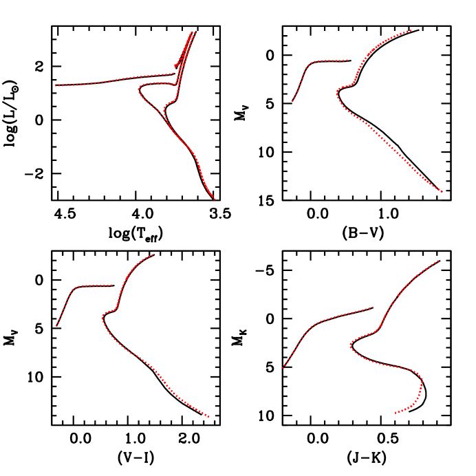
Figure 1: Top-left panel: HRD of solar scaled (solid lines) and $\alpha$-enhanced (dotted lines) isochrones for [M/H]=$-$1.40, $Y$=0.2478, and ages equal to 2 and 12 Gyr, respectively. The 12 Gyr isochrones are plotted up to the tip of the RGB, together with the corresponding ZAHBs. Top-right panel: Optical $BV$ CMD of the 12 Gyr, [M/H]=$-$1.40 solar scaled (solid lines) and $\alpha$-enhanced (dotted lines) isochrones and ZAHBs. Bottom-left panel: Optical $VI$ CMD of the 12 Gyr, [M/H]=$-$1.40 solar scaled (solid lines) and $\alpha$-enhanced (dotted lines) isochrones and ZAHBs. Bottom-right panel: Infrared $JK$ CMD of the 12 Gyr, [M/H]=$-$1.40 solar scaled (solid lines) and $\alpha$-enhanced (dotted lines) isochrones and ZAHBs.

Differences in the HRD are at most equal to 1% in $T_{\mathrm{e}ff}$, and about 5% in luminosity (0.02 dex) around the TO and along the ZAHB ($\alpha$-enhanced isochrones being hotter and brighter). This good agreement is preserved in the $VI$ and $JK$ CMDs, apart from the MS for masses below about 0.5$M_{\odot}$, where the $\alpha$-enhanced isochrones are systematically redder than the solar scaled ones by at most 0.07 mag in $(V-I)$, and bluer by at most 0.03 mag in $(J-K)$ (the lower MS wasn’t explored by Cassisi et al. (2004)). The TO and ZAHB magnitudes of the $\alpha$-enhanced isochrones are typically just about 0.04-0.05 mag brighter. In the $BV$ CMD the $\alpha$-enhanced isochrones are systematically bluer by about 0.04 mag on average.

We also find that these colour differences increase when moving to CMDs involving shorter wavelength filters like $U$, consistent with the results by Cassisi et al. (2004).

4 Comparison with other model libraries

We compare here our new $\alpha$-enhanced isochrones to the previous $\alpha$-enhanced BaSTI release (more specifically, the isochones calculated with the Reimers parameter $\eta$=0.4 Pietrinferni et al., 2006) and the DSEP (Dotter et al., 2008a) $\alpha$-enhanced models (comparisons of the previous BaSTI release with earlier $\alpha$-enhanced model libraries are discussed in Pietrinferni et al., 2006). Comparisons are made in the theoretical HRD, to avoid additional differences introduced by the choice of the BCs, and we focus on old ages, typical of $\alpha$-enhanced stellar populations.

Figures 2 and  3 show the HRD of isochrones with ages equal to 10 and 14 Gyr and, respectively, [Fe/H]=$-1.9$ and [Fe/H]=$-0.7$, from both our new calculations and Pietrinferni et al. (2006). At each [Fe/H] the initial $Y$ of the two sets of isochrones is the same within less than 1%; the values of $Z$ are however much less similar, due to the different solar heavy element distributions. At [Fe/H]=$-1.9$ our new models have an initial $Z=0.0004$, compared to $Z=0.0006$ in Pietrinferni et al. (2006) calculations, while at [Fe/H]=$-0.7$ the new calculations have an initial $Z$=0.006, compared to $Z$=0.008 in the old BaSTI release. Another difference between the two sets of isochrones arises from the inclusion of atomic diffusion in these new calculations, which wasn’t accounted for in Pietrinferni et al. (2006) models, with the exception of the solar model computation to calibrate the mixing length and the initial solar helium abundance (see, Pietrinferni et al., 2004, 2006, for more details).

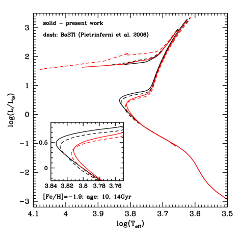
Figure 2: HRD of 10 and 14 Gyr, [Fe/H]=$-1.9$ isochrones for our new calculations (solid lines) and the previous BaSTI $\alpha$-enhanced release (Pietrinferni et al., 2006). The inset shows an enlargement of the MS turn off region.

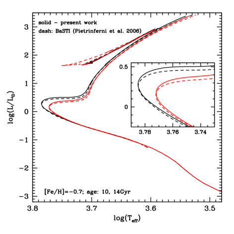
Figure 3: As Fig. 2 but for [Fe/H]=$-0.7$ isochrones.

The MS section of the new isochrones (extended to much lower masses compared to Pietrinferni et al., 2006) is slightly hotter, due to the lower initial $Z$, but around the MS turn off (TO) the differences increase and are metallicity- and age-dependent: This is due to the combined effect of the inclusion of atomic diffusion in our new calculations, differences in the nuclear cross sections for the H-burning discussed in Hidalgo et al. (2018), and the different initial $Z$. As a result, the isochrone TO luminosity is generally higher in these new calculations, whilst the TO effective temperature is higher at the younger age and cooler at the older age displayed. These differences decrease with increasing metallicity (a higher metallicity decreases the effect of atomic diffusion from the convective envelopes, because of the more massive outer convective region).

As for the RGB, the new isochrones are systematically hotter than Pietrinferni et al. (2006), mainly due to the lower initial $Z$, a result consistent with the comparisons of the solar scaled isochrones (Hidalgo et al., 2018). The difference in $T_{\mathrm{e}ff}$ increases with increasing [Fe/H]: It is on the order of 20-30 K at [Fe/H]=$-$1.9, increasing up to $\sim$120 K at [Fe/H]=$-$0.7.

The core He-burning stage in the new isochrones is generally shifted to hotter $T_{\mathrm{e}ff}$ and higher luminosities. These differences are caused by the lower mass in Pietrinferni et al. (2006) isochrones, caused by a larger value of the Reimers parameter $\eta$ ($\eta$=0.4 against $\eta=0.3$ in the new calculations) and a brighter tip of the RGB (TRGB), that increases further the amount of mass lost along the RGB.

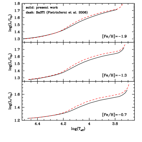
Figure 4: HRD of ZAHB models from our new calculations and from Pietrinferni et al. (2006) –solid and dashed lines, respectively– for the three labelled values of [Fe/H]. The minimum and maximum mass of the ZAHB models is the same in the two datasets (see text for more details).

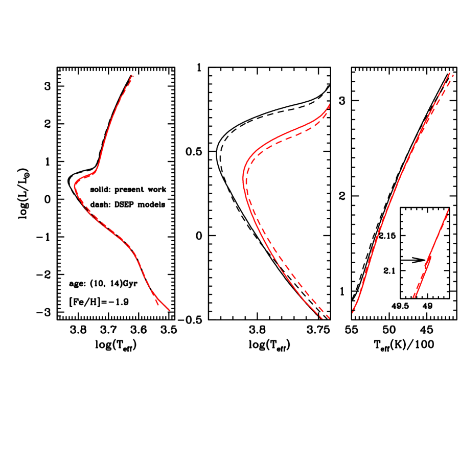
Figure 5: Left panel: HRD of 10 and 14 Gyr, [Fe/H]=$-1.9$ isochrones from the DSEP database, (dashed lines – Dotter et al., 2008a) and our new calculations (solid lines). Middle panel: An enlargement of the TO region of the isochrones. Right panel: Enlargement of the RGB portion of the isochrones. The inset shows the RGB bump region in the 14 Gyr isochrones; the arrow marks the location of the RGB bump in our calculations.

To explain more thoroughly the results of this comparison of core He-burning isochrones, it is helpful to study the corresponding ZAHB models. Figure 4 shows the HRD of ZAHB models (obtained from progenitors with an age of 12.5 Gyr at the TRGB) in our new calculations and Pietrinferni et al. (2006). A lower total mass shifts the ZAHB models towards hotter effective temperatures, hence lower luminosities, and this explains why the core He-burning Pietrinferni et al. (2006) isochrones, with a lower evolving mass, are fainter than our new isochrones despite a generally brighter ZAHB at fixed $T_{\mathrm{e}ff}$.

To understand why the ZAHB luminosities of new and old calculations are different, three points need to be taken into account. First, the new calculations include atomic diffusion, whose impact on ZAHB models has been extensively investigated by Cassisi et al. (1998) (see also Cassisi & Salaris, 2013, and references therein). Atomic diffusion increases the mass of the He-core at He ignition for a given initial chemical composition, and decreases the He abundance in the envelope. The second point is that the improved electron conduction opacities employed in these new calculations decrease the size of the He-core at He ignition, compared to Pietrinferni et al. (2006) models (for a detailed discussion on this point we refer to Cassisi et al., 2007; Hidalgo et al., 2018). Finally, at a given [Fe/H], the new ZAHB models have a lower initial $Z$, because of the different solar metal distribution.

At the hot end of the ZAHB, above about 16,000 K, it is the He-core mass that controls the luminosity, and here old and new calculations have roughly the same luminosity; this happens because the increase of the He-core mass due to the inclusion of diffusion in the new models, approximately balances the decrease caused by the updated electron conduction opacities. At lower effective temperatures the H-burning shell also contributes to the ZAHB luminosity, and the situation is different: In this regime, despite the higher metallicity that tends to make the ZAHB fainter, the old BaSTI calculations are systematically brighter than the new models, by about $\Delta\log(L/L_{\odot})=0.02-0.04$ dex at the level of the RR Lyrae instability strip. This difference is driven by the reduction of the helium content of the envelope due to the inclusion of atomic diffusion (that decreases the energy generation efficiency of the H-burning shell) in the new models, together with the reduced He-core mass caused by the improved electron conduction opacities.

The average mass of the new ZAHB models within the RR Lyrae instability strip ($M_{RR}$) taken at $\log(T_{\mathrm{e}ff})=3.83$, is also different from Pietrinferni et al. (2006) models. At [Fe/H]=$-1.9$ our new models give $M_{RR}$=$0.675M_{\odot}$ compared to $0.72M_{\odot}$ in Pietrinferni et al. (2006), whilst at [Fe/H]=$-1.3$, the new calculations provide $M_{RR}$=$0.635M_{\odot}$ against $\sim 0.615M_{\odot}$ for the old release. At [Fe/H]=$-0.7$ we get $M_{RR}=0.58M_{\odot}$, while $M_{RR}=0.568M_{\odot}$ in Pietrinferni et al. (2006) models.

Next, we compare our new isochrones up to the TRGB with the DSEP ones (Dotter et al., 2008a), for the same [Fe/H] and age values of the comparison with Pietrinferni et al. (2006). These isochrones have been downloaded from the DSEP web tool, 2012 version, choosing the models with [$\alpha$/Fe]=+0.4, as in our calculations. DSEP models also include atomic diffusion without radiative levitation, but there are differences in the physics inputs, most notably boundary conditions, electron conduction opacities, and also the details of the EOS. Despite also a different reference solar heavy element distribution (Grevesse & Sauval, 1998) and a higher $\Delta{Y}/\Delta{Z}$, initial metallicities ($Z$=0.00041 and $Z$=0.0065) and helium mass fractions ($Y$=0.2457 and $Y$=0.2555, respectively) are very close to our values in these comparisons.

At [Fe/H]=$-1.9$ the two sets of isochrones are very similar, as shown in Fig. 5. The MS of DSEP calculations is slightly cooler, the TO luminosity is essentially the same, while the subgiant branch of our calculations is slightly brighter. Along the RGB the DSEP isochrones have a different slope; they start hotter than ours at the base of the RGB, to become cooler than our isochrones at higher luminosities, but $T_{\mathrm{e}ff}$ differences are small, within $\pm$50 K. The inset in the right panel of Fig. 5 shows the RGB bump region along the 14 Gyr old isochrones, that cannot be detected in the DSEP isochrone, likely due to the sparse sampling of the RGB.

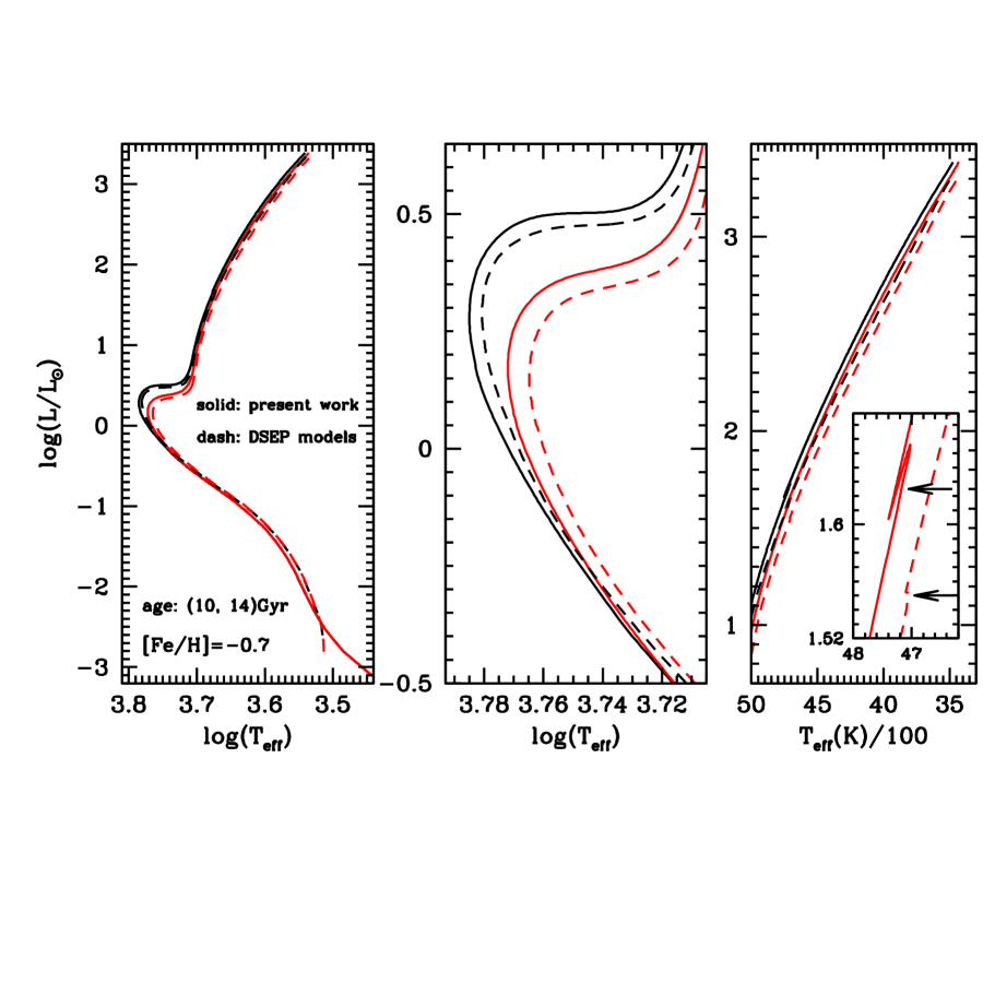
Figure 6: As Fig. 5 but for [Fe/H]=$-0.7$. At this metallicity, the RGB bump can be identified also in the DSEP isochrone, and it is marked by an arrow.

The situation is similar at [Fe/H]=$-$0.7, as shown by Fig.6, but the $T_{\mathrm{e}ff}$ differences along the MS and at the TO are slightly amplified at this higher metallicity. On the RGB the DSEP isochrones are this time systematically cooler than ours, by $\sim 60-80$ K, and the RGB bump in the 14 Gyr old isochrone is fainter than our results by $\Delta\log(L/L_{\odot})\sim 0.06$ dex.

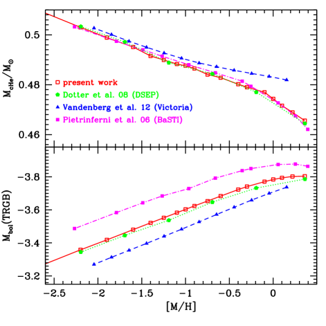
Figure 7: Upper panel: TRGB He-core mass (${M_{cHe}}$) as a function of the total metallicity [M/H] for an age of $\sim 12.5$ Gyr, taken from the labelled model libraries. Lower panel: As the upper panel but for the bolometric luminosity of the TRGB. The value $M_{Bol,\odot}=4.74$ of the absolute bolometric magnitude of the Sun has been adopted for all model libraries.

Table 4: Initial mass $M_{ini}$, actual mass $M_{fin}$, bolometric luminosity, effective temperature, He-core mass, and absolute magnitudes in the $I$, $J$, $H$, $K$ filters as a function of [Fe/H], for the TRGB of our 12.5 Gyr isochrones.

[Fe/H]	$M_{ini}(M_{\odot})$	$M_{fin}(M_{\odot})$	$\log(L_{\mathrm{T}RGB}/L_{\odot})$	$\log{T_{\mathrm{e}ff}}$	$M_{cHe}(M_{\odot})$	$M_{I}$	$M_{J}$	$M_{H}$	$M_{K}$
$-3.20$	0.801	0.715	3.180	3.651	0.5130	$-3.88$	$-4.69$	$-5.32$	$-5.42$
$-2.50$	0.800	0.706	3.239	3.646	0.5030	$-4.02$	$-4.85$	$-5.51$	$-5.60$
$-2.20$	0.801	0.701	3.264	3.637	0.4989	$-4.07$	$-4.93$	$-5.62$	$-5.72$
$-1.90$	0.806	0.699	3.288	3.623	0.4951	$-4.09$	$-5.01$	$-5.77$	$-5.87$
$-1.70$	0.812	0.699	3.305	3.612	0.4915	$-4.09$	$-5.07$	$-5.87$	$-5.98$
$-1.55$	0.818	0.701	3.317	3.603	0.4899	$-4.10$	$-5.11$	$-5.96$	$-6.07$
$-1.40$	0.826	0.703	3.329	3.592	0.4883	$-4.08$	$-5.15$	$-6.04$	$-6.17$
$-1.30$	0.833	0.707	3.337	3.585	0.4876	$-4.07$	$-5.18$	$-6.10$	$-6.24$
$-1.20$	0.840	0.711	3.345	3.577	0.4865	$-4.06$	$-5.21$	$-6.16$	$-6.31$
$-1.05$	0.855	0.720	3.357	3.566	0.4841	$-4.04$	$-5.26$	$-6.24$	$-6.41$
$-0.90$	0.874	0.735	3.369	3.555	0.4828	$-4.01$	$-5.31$	$-6.32$	$-6.50$
$-0.70$	0.905	0.759	3.385	3.537	0.4802	$-3.95$	$-5.39$	$-6.44$	$-6.65$
$-0.60$	0.923	0.775	3.392	3.528	0.4790	$-3.91$	$-5.43$	$-6.50$	$-6.72$
$-0.40$	0.967	0.818	3.404	3.511	0.4770	$-3.81$	$-5.52$	$-6.61$	$-6.86$
$-0.30$	0.981	0.830	3.410	3.501	0.4743	$-3.75$	$-5.57$	$-6.67$	$-6.93$
$-0.20$	1.003	0.853	3.414	3.492	0.4716	$-3.68$	$-5.61$	$-6.72$	$-7.00$
$-0.08$	1.027	0.879	3.417	3.481	0.4689	$-3.59$	$-5.67$	$-6.78$	$-7.07$
$+0.06$	1.054	0.908	3.418	3.468	0.4656	$-3.46$	$-5.72$	$-6.83$	$-7.15$

Figure 7 shows bolometric magnitude and He-core mass at the TRGB (${M_{cHe}}$) of our new isochrones, compared with the values from Pietrinferni et al. (2006), DSEP, and Victoria (VandenBerg et al., 2012) models at a reference age of 12.5 Gyr, as a function of the total metallicity [M/H]. We use [M/H] in this comparison to minimize the effect of different reference solar heavy element distributions and [$\alpha$/Fe]. There are however several differences in physics inputs and initial $Y$ among these sets of models.

The values of $M_{cHe}$ in our new models and Pietrinferni et al. (2006) results are very similar, with a difference of only about 0.002 $M_{\odot}$ between [M/H]$\sim-$1.6 and [M/H]$\sim-$0.3, the previous BaSTI values being higher. In general, the models compared in Fig. 7 display $M_{cHe}$ values within about $\pm$0.004 $M_{\odot}$ around our results, the exception being Victoria models, which for [M/H]$>-$0.9 provide increasingly higher values compared to ours. This latter behaviour is likely due to the assumption of constant $Y$ at all metallicities in the Victoria models, while all other calculations have $Y$ increasing with $Z$. An increase of $Y$ at fixed $Z$ tends to decrease ${M_{cHe}}$, and this explains at least qualitatively the comparison with Victoria models .

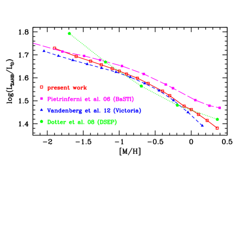
Figure 8: The luminosity of ZAHB models at the RR Lyrae instability strip (taken at $\log{T_{\mathrm{e}ff}}=3.83$), as a function of the total metallicity [M/H], from the labelled model libraries.

Regarding the TRGB, Fig. 7 shows that our new models are significantly fainter – by about $\sim 0.15$ mag at [M/H]=$-1.3$ – than the previous BaSTI predictions. This is partially due to the smaller He-core mass in the new calculations, but the main reason is the different reference solar metal distribution, and the inclusion of atomic diffusion. DSEP models are only slightly underluminous, and Victoria models are consistently fainter by about 0.1 mag, despite their larger ${M_{cHe}}$. This is partially due the different definition concerning $M_{cHe}$ as well as to the lower initial He abundance adopted in the Victoria model library.

As a reference, Table 4 reports several quantities at the TRGB as a function of [Fe/H] from our calculations, including ${M_{cHe}}$, the bolometric luminosity of the TRGB and absolute magnitudes in selected filters used for the TRGB distance scale (see next section).

Figure 8 compares the luminosity of our new ZAHB models at the RR Lyrae instability strip (taken at $\log{T_{\mathrm{e}ff}}=3.83$) with (Pietrinferni et al., 2006), DSEP and Victoria results, again as a function of the total metallicity [M/H]. Victoria models give results very close to ours (only slightly underluminous), whilst luminosities from the older BaSTI models are typically higher, with differences increasing for increasing [M/H]. DSEP models are much brighter at the lowest metallicities, then become close to our calculations. On the whole, at [M/H] between $\sim-$1.2 and 0.0, DSEP and Victoria models are consistent with our new results within about $\pm$0.02 dex. Table 5 summarizes some main properties of our ZAHB models at the RR Lyrae instability strip.

Table 5: Bolometric luminosity, absolute magnitudes in the $BVRIJHK$ filters, and the mass $M_{RR}$ of the ZAHB model at $\log{T_{\mathrm{e}ff}}=3.83$ –taken as representative of the average $T_{\mathrm{e}ff}$ within the RR Lyrae instability strip (Marconi et al., 2015)– as a function of [Fe/H].

[Fe/H]	$M_{RR}(M_{\odot})$	$\log(L_{\mathrm{Z}AHB}/L_{\odot})$	$M_{B}$	$M_{V}$	$M_{R}$	$M_{I}$	$M_{J}$	$M_{H}$	$M_{K}$
$-2.20$	0.791	1.728	0.709	0.42	0.20	$-0.03$	$-0.31$	$-0.52$	$-0.54$
$-1.90$	0.723	1.691	0.794	0.50	0.28	$~{}0.06$	$-0.22$	$-0.43$	$-0.45$
$-1.70$	0.687	1.670	0.847	0.55	0.33	$~{}0.11$	$-0.17$	$-0.38$	$-0.40$
$-1.55$	0.665	1.654	0.886	0.58	0.37	$~{}0.15$	$-0.13$	$-0.34$	$-0.37$
$-1.40$	0.646	1.641	0.915	0.61	0.39	$~{}0.17$	$-0.10$	$-0.31$	$-0.33$
$-1.30$	0.635	1.627	0.950	0.64	0.43	$~{}0.21$	$-0.07$	$-0.27$	$-0.30$
$-1.20$	0.624	1.615	0.979	0.67	0.45	$~{}0.23$	$-0.04$	$-0.24$	$-0.27$
$-1.05$	0.608	1.596	1.023	0.71	0.49	$~{}0.27$	$~{}0.00$	$-0.20$	$-0.23$
$-0.90$	0.596	1.574	1.086	0.76	0.54	$~{}0.33$	$~{}0.06$	$-0.15$	$-0.17$
$-0.70$	0.580	1.541	1.155	0.83	0.61	$~{}0.39$	$~{}0.13$	$-0.07$	$-0.09$
$-0.60$	0.573	1.520	1.227	0.88	0.66	$~{}0.45$	$~{}0.18$	$-0.01$	$-0.04$
$-0.40$	0.562	1.475	1.334	0.98	0.75	$~{}0.55$	$~{}0.28$	$~{}0.09$	$~{}0.06$
$-0.30$	0.555	1.458	1.404	1.03	0.81	$~{}0.60$	$~{}0.33$	$~{}0.14$	$~{}0.11$
$-0.20$	0.547	1.439	1.424	1.06	0.83	$~{}0.62$	$~{}0.36$	$~{}0.18$	$~{}0.15$
$-0.08$	0.539	1.413	1.483	1.11	0.88	$~{}0.67$	$~{}0.42$	$~{}0.24$	$~{}0.21$
$+0.06$	0.531	1.381	1.571	1.18	0.95	$~{}0.75$	$~{}0.49$	$~{}0.31$	$~{}0.29$

5 Comparisons with observations

In this section, we discuss results of a few tests to assess the general consistency of our new models and isochrones with selected observational constraints. In all of these comparisons, we have included the effect of extinction according to the standard Cardelli et al. (1989) reddening law, with $R_{V}\equiv A_{V}/E(B-V)$ = 3.1, and have calculated the ratios $A_{\lambda}/A_{V}$ for the relevant photometric filters, as described in Girardi et al. (2002)

The first test is shown in Fig. 9, which displays a comparison between the new theoretical $IJHK$ TRGB absolute magnitudes of Table 4, and the empirical results for 47 Tuc and $\omega$ Centauri by Bellazzini et al. (2004). Their derived absolute magnitudes for the TRGB of 47 Tuc have been shifted by +0.04 mag, to account for the new eclipsing binary distance by Thompson et al. (2020). The values for $\omega$ Centauri are unchanged, because already based on an eclipsing binary distance to this cluster (see discussion in Bellazzini et al., 2004). The metallicity assigned to $\omega$ Centauri is the [Fe/H] of the main cluster population, as discussed in Bellazzini et al. (2004). Our theoretical TRGB magnitudes appear nicely consistent with these results in all filters, within the corresponding error bars.

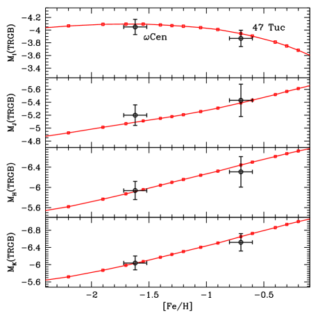
Figure 9: Comparison of the TRGB absolute magnitudes of our new calculations (see Table 4) with the $IJHK$ empirical results by Bellazzini et al. (2004) for the Galactic globular clusters 47 Tuc and $\omega$ Centauri (see text for details).

The following Fig.10 displays a comparison of the model ZAHB luminosities reported in Table 5 with the semiempirical results by de Santis & Cassisi (1999), based on the pulsational properties of RR Lyrae stars in GCs. Also in this case we find a general consistency with our models

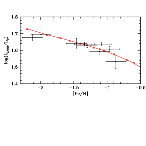
Figure 10: As Fig. 8, but showing our new calculations compared to the semiempirical results by de Santis & Cassisi (1999).

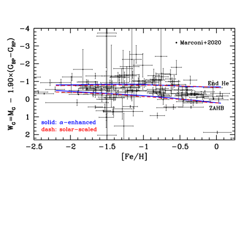
Figure 11: Wesenheit $W_{G}$ - [Fe/H] diagram of field RR Lyrae stars from Gaia data Release 2 Marconi et al. (2020) compared to the ZAHB and the sequence corresponding to the exhaustion of He in the center, for our $\alpha$-enhanced (solid lines) and solar scaled models (dashed lines – see text for details).

We have also compared our HB models with Gaia Data Release 2 results for a sample of Galactic field RR Lyrae stars with accurate parallaxes, magnitudes, and high-resolution spectroscopic measurements of [Fe/H], taken from Marconi et al. (2020) (their table A1). To remove uncertainties associated with both the poorly constrained extinction and $\alpha-$element enhancement, Fig. 11 shows the relation between the measured values of the reddening-free Wesenheit index $W_{G}=M_{G}-1.90\times(G_{BP}-G_{RP})$ (see Ripepi et al., 2019) and the iron abundance of the stars in the sample. This data is compared to the corresponding relationship - taken at $\log{T_{\mathrm{e}ff}}=3.83$ (see previous discussion) - predicted by both $\alpha$-enhanced and solar scaled (from Hidalgo et al., 2018) ZAHB models, that display almost identical $W_{G}$ values at fixed [Fe/H]. The evolution off-ZAHB of the tracks in the instability strip display a small increase of $W_{G}$ by at most $\sim$0.2 mag at intermediate and high [Fe/H], followed by a steady decrease until the exhaustion of central He (the sequences corresponding to the exhaustion of central He are also displayed). But for a few peculiar cases that would need to be analyzed individually, the large majority of the stars across the whole [Fe/H] range lie either slightly below (fainter $W_{G}$) the ZAHB –consistent with the evolutionary path of the tracks– or above it, as expected from the models. There are also several objects located above the sequences corresponding to the exhaustion of central He, but we refrain from speculating about their origin, given the large errors on $W_{G}$ that affect most of these stars.

A test with CMDs of the metal poor Galactic globular clusters (GGC) NGC 6397 ([Fe/H]=$-2.03\pm 0.05$,[$\alpha$/Fe]=0.34$\pm$0.02) (see Gratton et al., 2003) follows in Figs. 12 and  13. The first comparison is between our [Fe/H]=$-$1.9, $Y$=0.248 isochrones and ZAHB models, and the Johnson-Cousins $VI$ photometry by Stetson (2000), as shown in Fig. 12. The fit of the theoretical ZAHB and the lower MS to the observed CMD constrain distance modulus and reddening to $E(B-V)$=0.19 and $(m-M)_{0}$=11.96, respectively. The TO region is matched by a 13.5 Gyr isochrone, that is also nicely consistent with the observed RGB. These values of reddening and distance well agree with $E(B-V)=0.183\pm 0.005({\rm stat})\pm 0.011({\rm syst})$ estimated by Gratton et al. (2003), and $(m-M)_{0}=11.89\pm 0.07({\rm stat})\pm 0.09({\rm syst})$ determined by Brown et al. (2018), from measurements of the cluster parallax distance using the HST/WFC3 spatial-scanning mode.

Like most GGCs, stars in this cluster displays the well known O-Na and C-N abundance anticorrelations (see, e.g., Bastian & Lardo, 2018, for a review on the topic), usually associated also to a range of helium abundances. The anticorrelations do not affect isochrones and bolometric corrections in optical filters, but the initial helium abundance does, through its effect on model luminosities, lifetimes and $T_{\mathrm{e}ff}$ (see, e.g., Cassisi & Salaris, 2020, for a review). However, the He abundance spread is negligible in this cluster (as derived by Milone et al., 2018) and isochrones for a single, standard value of $Y$ are appropriate to match the observed CMD.

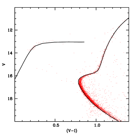
Figure 12: Comparison of a [Fe/H]=$-$1.9, 13.5 Gyr isochrone and ZAHB with $Y$=0.248 (solid line) with the Stetson (2000) $VI$ CMD of NGC 6397 (see text for details).

The deep HST/ACS optical CMD from Richer et al. (2008) is displayed in Fig. 13, together with the same isochrone of Fig. 12 but in the filter system of the ACS camera on board of HST, using the same distance moduls and reddening of the comparison in the Johnson-Cousins CMD. In this case, we note that between $\sim$1 and $\sim$5 $F606W$ magnitudes below the TO the isochrone is systematically bluer than the data; the same happens when $F606W$ is fainter than $\sim$7 magnitudes below the TO. While this latter discrepancy is found also for the higher metallicity example discussed below (see the discussion on 47 Tuc that will follow) the same is not true for the brighter magnitude range. The reason might be related to possible metallicity-dependent offsets of the bolometric corrections for the HST/ACS system, but comparisons with more clusters are required to reach a definitive conclusion.

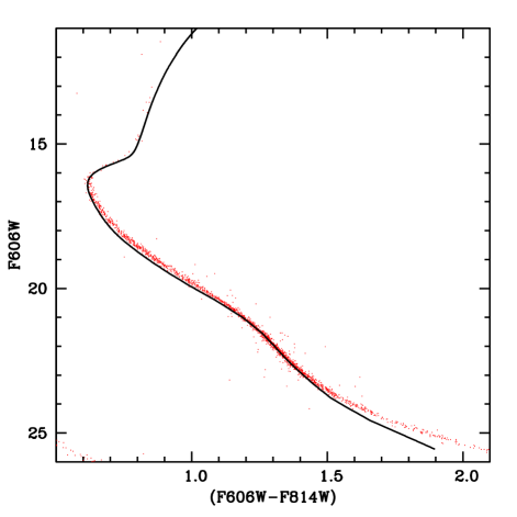
Figure 13: Comparison of a [Fe/H]=$-$1.9, 13.5 Gyr isochrone with $Y$=0.248 (solid line) with the HST/ACS CMD of NGC 6397 by Richer et al. (2008) (see text for details).

The next comparison is with the $BV$ CMD (from Bergbusch & Stetson, 2009) of the metal rich GGC 47 Tuc ([Fe/H]=$-0.66\pm 0.04$, [$\alpha$/Fe]=0.30$\pm$0.02) (see Gratton et al., 2003). This cluster has an internal He abundance spread with a range $\Delta Y\sim$0.03-0.05 (di Criscienzo et al., 2010; Salaris et al., 2016; Milone et al., 2018), and we use ZAHB and isochrones for both normal $Y$=0.255 and enhanced $Y$=0.300 helium. We fix simultaneously the distance modulus $(m-M)_{0}=13.30$ and reddening $E(B-V)$=0.02, by matching the lower envelope of the red HB and approximately the red edge of the lower MS, with ZAHB and isochrones for $Y$=0.255. We then tested that, for the same reddening and distance, the helium enhanced isochrones and ZAHB are still consistent with the observed sequences in the CMD. Figure 14 displays a comparison between the cluster CMD and 12.3 Gyr, [Fe/H]=$-$0.7, $Y$=0.255 and $Y$=0.300 isochrones, which match the position of the cluster TO, together with ZAHB models for both helium abundances. The derived value of $E(B-V)$ is in excellent agreement with $E(B-V)=0.024\pm 0.004({\rm stat})\pm 0.011({\rm syst})$ estimated by Gratton et al. (2003); the distance is fully consistent with the average $(m-M)_{0}=13.27\pm 0.07$ obtained from two cluster eclipsing binaries (Thompson et al., 2010, 2020).

Another empirical and independent distance determination for this cluster, based on Gaia Data Release 2 results, provides $(m-M)_{0}=13.24\pm 0.005({\rm stat})\pm 0.058({\rm sys})$ mag  (Chen et al., 2018), consistent with both our result and the eclipsing binary analysis.

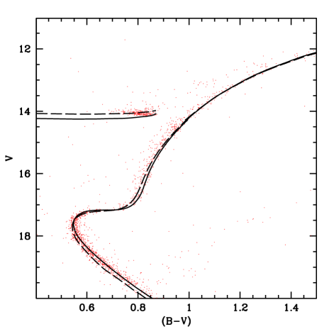
Figure 14: Fit of two [Fe/H]=$-$0.7, 12.3 Gyr isochrones and ZAHBs with $Y$=0.255 (solid line) and 0.300 (dashed line), respectively, to the Bergbusch & Stetson (2009) $BV$ CMD of 47 Tuc (see text for details).

Figure 15 displays the much deeper HST/ACS optical CMD by Kalirai et al. (2012) compared to the same isochrones of Fig. 14, using the same distance modulus and extinction. As for the case of the more metal poor cluster NGC 6397, the fainter part of the isochrone MS (for both values of the initial helium) is systematically bluer than the observations. To investigate this issue, we show in Fig. 16 the HST/WFC3 infrared CMD by Kalirai et al. (2012), compared only to the $Y$=0.255 isochrone, using again the same distance modulus and extinction of Fig. 14. In this CMD the isochrone does not appear systematically bluer than the data along the lower MS, and follows well the observed changing shape, due to the competition between the collision induced absorption of the ${\rm H_{2}}$ molecule in the infrared (that shifts the colours to the blue) and the increase of the radiative opacity with decreasing $T_{\mathrm{e}ff}$ (see, e.g., Cassisi & Salaris, 2013, and references therein). This suggests that the systematic difference between theory and observations found in optical colours might be due to the adopted bolometric corrections. Below $F160W\sim$18.5 the ($F110W-F160W$) colour is sensitive to the specific metal abundance patterns of the He-enhanced multiple populations hosted by the cluster, that affect the bolometric corrections. As shown by Milone et al. (2012), the result is to have redder colours at fixed $F160W$, compared to models with standard $\alpha$-enhanced composition.

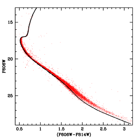
Figure 15: As Fig. 14 but for Kalirai et al. (2012) HST/ACS CMD (see text for details).

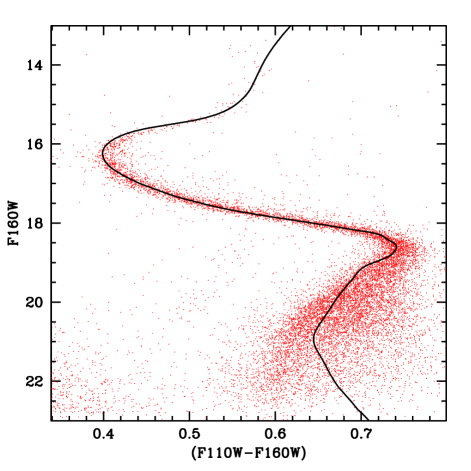
Figure 16: As Fig. 14 but for the HST/WFC3 infrared CMD by Kalirai et al. (2012). Only the $Y$=0.255 isochrone is shown (see text for details).

Figure 17 shows the 12.3 Gyr $Y$=0.255 isochrone in a mass-radius diagram, compared to the masses and radii of the components of the two cluster eclipsing binaries. The age determined from the CMD is nicely consistent with the radius of the eclipsing binary components. The isochrone for $Y$=0.300 lies outside the boundaries of this diagram, shifted to masses too low to be consistent with the data.

Figure 17: Comparison of an isochrone for a [Fe/H]=$-$0.7, $Y$=0.255, 12.3 Gyr, with data for the cmponents of two eclipsing binaries in 47 Tuc, in a mass-radius diagram (see text for details).

6 Conclusions

We have presented an overview of the updated BaSTI $\alpha$-enhanced models, whose input physics and reference solar metal mixture are consistent with the updated solar scaled models of Paper I. Like for the new solar scaled models, the updated $\alpha$-enhanced library increases significantly the number of available metallicities, includes the very low-mass star regime, accounts consistently for the pre-MS evolution in the isochrone calculations, and also provides the asteroseismic properties of the models.

We successfully tested these new calculations against the luminosities of the ZAHB and TRGB in selected GGCs. We also compared the isochrones with CMDs of one metal rich (47 Tuc) and one metal poor (NGC 6397) GGC; they provide a good fit to the observed CMDs, for distance moduli consistent with both the parallax and eclipsing binary distance to 47 Tuc, and the parallax distance to NGC 6397. The best fit isochrone for 47 Tuc can also nicely match the mass-radius diagram of the components of two cluster eclipsing binaries.

Like for the updated solar scaled library, the entire $\alpha$-enhanced database is publicly available at the following dedicated websites: http://basti-iac.oa-abruzzo.inaf.it and https://basti-iac.iac.es. Here we include stellar evolution tracks and isochrones in several photometric systems, and the asteroseismic properties of our grid of stellar evolution calculations. We can also provide, upon request, additional calculations (both evolutionary and asteroseismic outputs) for masses not included in our standard grids. These websites include also a web-tool to calculate online synthetic CMDs for any arbitrary star formation history and age metallicity relation, using the updated BaSTI isochrones. Details about the inputs to specify when running this web-tool, as well as a detailed discussion of the outputs, are provided in the Appendix.

Appendix A Synthetic color-magnitude diagram tool at BaSTI web site.

As for the previous release of the library, the new BaSTI website contains a tool for the computation of synthetic CMDs (http://basti-iac.oa-teramo.inaf.it/syncmd.html). This tool can be used after requesting a user ID to the BaSTI-IAC team members by using the link http://basti-iac.oa-abruzzo.inaf.it/requests.html. Here we provide information about the inputs and how the code works. The user has to select among a combination of heavy element mixtures (solar scaled or $\alpha$-enhanced) and available grids of models (various options about overshooting, diffusion and mass loss). Variations of the He abundance at fixed metallicity cannot yet be considered, but this is a feature that will be implemented in the near future. The user can also choose to identify the radial pulsators in the synthetic population, and determine their type and pulsation periods.

After this selection, two sets of input parameters are requested: Star-formation history (SFH) and photometric input parameters. SFH input parameters are as follows:

• Age: A list of ages $t_{i}$ (in Myr, older age first, with age = 0 denoting stars that are forming now). A maximum of 50 age values are allowed.

• SFR: Relative star formation rate at each age. The code rescales the individual values to the maximum one provided.

• Metallicity: [Fe/H] of stars formed at each $t_{i}$.

• Metallicity spread: 1 sigma Gaussian spread (in dex) around each metallicity.

• SFR scale: This number (the maximum value allowed is equal to $2\times 10^{6}$) is multiplied by the value of the SFR to provide the number of stars formed between age $t_{i}$ and age $t_{i+1}$.

• Low mass: Lower stellar mass mass (in units of $\rm M_{\odot}$) to be included in the calculations (between $0.1~{}\rm M_{\odot}$ and $120~{}\rm M_{\odot}$).

• Binaries: Fraction of unresolved binaries. If the fraction is different from zero the mass of the second component is selected randomly following Woo et al. (2003), and the fluxes of the two unresolved components are properly added.

• Mass ratio: Minimum mass ratio for binary systems (upper value is 1.0).

• IMF: Initial mass function type (0 for a single power law, 1 for Kroupa et al. (1993)). If a single power law is selected, the slope must be given (e.g.: -2.35).

• Variables: If a value equal to 1 is assigned to this parameter, the code identifies the radial pulsators in the synthetic population, and calculates their properties. A value equal to 0 makes the code skip the identification of radial pulsators.

• Random 1 and 2: Seeds for the Monte Carlo number generator. The system will generate these numbers automatically if none are given.

The photometric input parameters are:

• Photometric error: Mean photometric error (mag.)

• Photometric error type: None, constant, or error table.

• Photometric system: Select one of the photometric systems available.

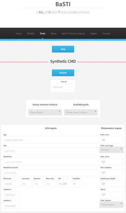
Figure 18: Synthetic CMD web-tool at BaSTI website.

The code computes the synthetic CMD as follows: For each age $t_{i}$, the number of stars formed between $t_{i}$ and $t_{i+1}$ is obtained by the multiplying the SFR scale by the value of the SFR at $t_{i}$. For each star born in this age interval, a random age t ($t_{i}\leq t<t_{i+1}$) is drawn from a flat probability distribution, together with a mass $m$ selected according to the specified IMF, and the corresponding value of $\rm[Fe/H]_{i}$. If a value different from zero for $\rm\sigma([Fe/H]_{i})$ is specified, then $\rm[Fe/H]_{i}$is perturbed using a Gaussian probability distribution centered in $\rm[Fe/H]_{i}$ and sigma = $\rm\sigma([Fe/H]_{i})$. With these three values of $t$, $m$, and [Fe/H] the program interpolates quadratically in age, metallicity and mass among the isochrones in the grid, to calculate the star’s photometric properties, plus luminosity and effective temperature. The code also checks whether the synthetic star is located within the instability strip (IS) for radial pulsations, by comparing its position in the HRD with the boundaries of the IS predicted by accurate pulsation models of RR Lyrae stars (see, Marconi et al., 2015, and references therein), anomalous Cepheids (Fiorentino et al., 2006), and classical Cepheids (Fiorentino et al., 2007; De Somma et al., 2020). If the star is located within a given IS, the corresponding pulsation period is calculated by using the appropriate theoretical relationship (see the previous references) between period, luminosity, effective temperature, mass and metallicity.

Once all stars formed between ages $t_{i}$ and $t_{i+1}$ are generated, the next time interval is considered and the cycle is repeated, ending when all stars in the final age bin between $t_{n-1}$ and $t_{n}$ are generated. The values of the SFR and [Fe/H] at $t_{n}$ are not considered and can be set to any arbitrary number. To compute the synthetic CMD of a single-age stellar population, just one age value needs to be provided as input. The BaSTI website provides some examples of SFHs and the corresponding web-tool inputs.

Once a run is completed, the user will receive an email with instructions to download two files: One with the synthetic stars, and another with the integrated properties of the population. The content of the first file is as follows:

• column 1: Star number (+2 if unresolved binary);

• column 2: Logarithm of the age in years;

• column 3: [Fe/H];

• column 4: Value of the current stellar mass in $\rm M_{\odot}$;

• column 5: log($L/L_{\odot}$);

• column 6: log($T_{\mathrm{e}ff}$);

• column 7: Initial mass of the unresolved secondary star ($\rm M_{\odot}$) if different from 0.0;

• column 8: Index that denotes the type of radial pulsator. A value equal to 0 stands for no pulsations, 1 corresponds to fundamental-mode RR Lyraes, 2 identifies the first overtone RR Lyraes, 3 corresponds to fundamental-mode anomalous Cepheids, 4 labels the first overtone anomalous Cepheids,; 5 denotes fundamental-mode classical Cepheids;

• column 9: log(P), with $P$ being the period of pulsations (in days). It is set to 99.99 if the synthetic star does not pulsate (see previous discussion);

• column 10 to the end: Absolute magnitudes in the selected photometric system.

The integrated properties file contains the following information:

• Integrated magnitudes in all bands for the selected photometric system.

• Total mass of formed stars ($\rm M_{\odot}$).

• Number of stars evolving in the synthetic CMD, including unresolved stars companions.

• Number of fundamental-mode RR-Lyrae stars.

• Number of first overtone RR-Lyrae stars.

• Number of fundamental-mode anomalous Cepheids.

• Number of first overtone anomalous Cepheids.

• Number of fundamental-mode classical Cepheids

References

- Allard et al. (2012) Allard, F., Homeier, D., & Freytag, B. 2012, Philosophical Transactions of the Royal Society of London Series A, 370, 2765
- Bastian & Lardo (2018) Bastian, N., & Lardo, C. 2018, ARA&A, 56, 83
- Bellazzini et al. (2004) Bellazzini, M., Ferraro, F. R., Sollima, A., Pancino, E., & Origlia, L. 2004, A&A, 424, 199
- Bergbusch & Stetson (2009) Bergbusch, P. A., & Stetson, P. B. 2009, AJ, 138, 1455
- Bergemann & Serenelli (2014) Bergemann, M., & Serenelli, A. 2014, Solar Abundance Problem, ed. E. Niemczura, B. Smalley, & W. Pych, 245–258
- Bessell & Murphy (2012) Bessell, M., & Murphy, S. 2012, PASP, 124, 140
- Bessell (1990) Bessell, M. S. 1990, PASP, 102, 1181
- Bessell (2011) —. 2011, Astronomical Society of the Pacific Conference Series, Vol. 451, Science with the Skymapper Telescope, ed. S. Qain, K. Leung, L. Zhu, & S. Kwok, 323
- Bessell & Brett (1988) Bessell, M. S., & Brett, J. M. 1988, PASP, 100, 1134
- Bessell et al. (1998) Bessell, M. S., Castelli, F., & Plez, B. 1998, A&A, 333, 231
- Brown et al. (2018) Brown, T. M., Casertano, S., Strader, J., et al. 2018, ApJ, 856, L6
- Cabrera-Ziri et al. (2020) Cabrera-Ziri, I., Speagle, J. S., Dalessandro, E., et al. 2020, MNRAS, 495, 375
- Caffau et al. (2011) Caffau, E., Ludwig, H.-G., Steffen, M., Freytag, B., & Bonifacio, P. 2011, Sol. Phys., 268, 255
- Cardelli et al. (1989) Cardelli, J. A., Clayton, G. C., & Mathis, J. S. 1989, ApJ, 345, 245
- Cassisi et al. (1998) Cassisi, S., Castellani, V., degl’Innocenti, S., & Weiss, A. 1998, A&AS, 129, 267
- Cassisi et al. (2007) Cassisi, S., Potekhin, A. Y., Pietrinferni, A., Catelan, M., & Salaris, M. 2007, ApJ, 661, 1094
- Cassisi & Salaris (2013) Cassisi, S., & Salaris, M. 2013, Old Stellar Populations: How to Study the Fossil Record of Galaxy Formation
- Cassisi & Salaris (2020) —. 2020, A&A Rev., 28, 5
- Cassisi et al. (2004) Cassisi, S., Salaris, M., Castelli, F., & Pietrinferni, A. 2004, ApJ, 616, 498
- Cayrel de Strobel et al. (1997) Cayrel de Strobel, G., Crifo, F., & Lebreton, Y. 1997, in ESA Special Publication, Vol. 402, Hipparcos - Venice ’97, ed. R. M. Bonnet, E. Høg, P. L. Bernacca, L. Emiliani, A. Blaauw, C. Turon, J. Kovalevsky, L. Lindegren, H. Hassan, M. Bouffard, B. Strim, D. Heger, M. A. C. Perryman, & L. Woltjer, 687–688
- Chen et al. (2018) Chen, S., Richer, H., Caiazzo, I., & Heyl, J. 2018, ApJ, 867, 132
- Christensen-Dalsgaard (2008) Christensen-Dalsgaard, J. 2008, Ap&SS, 316, 113
- Cohen et al. (2003) Cohen, M., Wheaton, W. A., & Megeath, S. T. 2003, AJ, 126, 1090
- Cordier et al. (2007) Cordier, D., Pietrinferni, A., Cassisi, S., & Salaris, M. 2007, AJ, 133, 468
- de Santis & Cassisi (1999) de Santis, R., & Cassisi, S. 1999, MNRAS, 308, 97
- De Somma et al. (2020) De Somma, G., Marconi, M., Molinaro, R., et al. 2020, ApJS, 247, 30
- di Criscienzo et al. (2010) di Criscienzo, M., Ventura, P., D’Antona, F., Milone, A., & Piotto, G. 2010, MNRAS, 408, 999
- Doi et al. (2010) Doi, M., Tanaka, M., Fukugita, M., et al. 2010, AJ, 139, 1628
- Dotter et al. (2007) Dotter, A., Chaboyer, B., Ferguson, J. W., et al. 2007, ApJ, 666, 403
- Dotter et al. (2008a) Dotter, A., Chaboyer, B., Jevremović, D., et al. 2008a, ApJS, 178, 89
- Dotter et al. (2008b) —. 2008b, ApJS, 178, 89
- Fiorentino et al. (2006) Fiorentino, G., Limongi, M., Caputo, F., & Marconi, M. 2006, A&A, 460, 155
- Fiorentino et al. (2007) Fiorentino, G., Marconi, M., Musella, I., & Caputo, F. 2007, A&A, 476, 863
- Fu et al. (2018) Fu, X., Bressan, A., Marigo, P., et al. 2018, MNRAS, 476, 496
- Gaia Collaboration et al. (2020) Gaia Collaboration, Brown, A. G. A., Vallenari, A., et al. 2020, arXiv e-prints, arXiv:2012.01533
- Girardi et al. (2002) Girardi, L., Bertelli, G., Bressan, A., et al. 2002, A&A, 391, 195
- Gratton et al. (2019) Gratton, R., Bragaglia, A., Carretta, E., et al. 2019, A&A Rev., 27, 8
- Gratton et al. (2003) Gratton, R. G., Bragaglia, A., Carretta, E., et al. 2003, A&A, 408, 529
- Grevesse & Sauval (1998) Grevesse, N., & Sauval, A. J. 1998, Space Sci. Rev., 85, 161
- Groenewegen (2006) Groenewegen, M. A. T. 2006, A&A, 448, 181
- Hauschildt & Baron (1999) Hauschildt, P. H., & Baron, E. 1999, Journal of Computational and Applied Mathematics, 109, 41
- Hayes et al. (2018) Hayes, C. R., Majewski, S. R., Shetrone, M., et al. 2018, ApJ, 852, 49
- Hidalgo et al. (2018) Hidalgo, S. L., Pietrinferni, A., Cassisi, S., et al. 2018, ApJ, 856, 125
- Husser et al. (2013) Husser, T.-O., Wende-von Berg, S., Dreizler, S., et al. 2013, A&A, 553, A6
- Jordi et al. (2010) Jordi, C., Gebran, M., Carrasco, J. M., et al. 2010, A&A, 523, A48
- Kalirai et al. (2012) Kalirai, J. S., Richer, H. B., Anderson, J., et al. 2012, AJ, 143, 11
- Kim et al. (2002) Kim, Y.-C., Demarque, P., Yi, S. K., & Alexand er, D. R. 2002, ApJS, 143, 499
- Korn et al. (2007) Korn, A. J., Grundahl, F., Richard, O., et al. 2007, ApJ, 671, 402
- Kroupa et al. (1993) Kroupa, P., Tout, C. A., & Gilmore, G. 1993, MNRAS, 262, 545
- Kurucz (1970) Kurucz, R. L. 1970, SAO Special Report, 309
- Maíz Apellániz (2006) Maíz Apellániz, J. 2006, AJ, 131, 1184
- Maíz Apellániz (2017) Maíz Apellániz, J. 2017, A&A, 608, L8
- Maíz Apellániz & Weiler (2018) Maíz Apellániz, J., & Weiler, M. 2018, A&A, 619, A180
- Marconi et al. (2020) Marconi, M., Molinaro, R., Ripepi, V., et al. 2020, arXiv e-prints, arXiv:2011.06675
- Marconi et al. (2015) Marconi, M., Coppola, G., Bono, G., et al. 2015, ApJ, 808, 50
- Mashonkina et al. (2019) Mashonkina, L. I., Neretina, M. D., Sitnova, T. M., & Pakhomov, Y. V. 2019, Astronomy Reports, 63, 726
- Miglio et al. (2012) Miglio, A., Brogaard, K., Stello, D., et al. 2012, MNRAS, 419, 2077
- Milone et al. (2012) Milone, A. P., Marino, A. F., Cassisi, S., et al. 2012, ApJ, 754, L34
- Milone et al. (2018) Milone, A. P., Marino, A. F., Renzini, A., et al. 2018, MNRAS, 481, 5098
- Mucciarelli et al. (2011) Mucciarelli, A., Salaris, M., Lovisi, L., et al. 2011, MNRAS, 412, 81
- Nieuwenhuijzen & de Jager (1990) Nieuwenhuijzen, H., & de Jager, C. 1990, A&A, 231, 134
- Pietrinferni et al. (2004) Pietrinferni, A., Cassisi, S., Salaris, M., & Castelli, F. 2004, ApJ, 612, 168
- Pietrinferni et al. (2006) —. 2006, ApJ, 642, 797
- Pietrinferni et al. (2013) Pietrinferni, A., Cassisi, S., Salaris, M., & Hidalgo, S. 2013, A&A, 558, A46
- Pietrinferni et al. (2009) Pietrinferni, A., Cassisi, S., Salaris, M., Percival, S., & Ferguson, J. W. 2009, ApJ, 697, 275
- Poole et al. (2008) Poole, T. S., Breeveld, A. A., Page, M. J., et al. 2008, MNRAS, 383, 627
- Ramírez et al. (2012) Ramírez, I., Meléndez, J., & Chanamé, J. 2012, ApJ, 757, 164
- Reimers (1975) Reimers, D. 1975, Memoires of the Societe Royale des Sciences de Liege, 8, 369
- Richard et al. (2002) Richard, O., Michaud, G., Richer, J., et al. 2002, ApJ, 568, 979
- Richer et al. (2008) Richer, H. B., Dotter, A., Hurley, J., et al. 2008, AJ, 135, 2141
- Ripepi et al. (2019) Ripepi, V., Molinaro, R., Musella, I., et al. 2019, A&A, 625, A14
- Rubele et al. (2012) Rubele, S., Kerber, L., Girardi, L., et al. 2012, A&A, 537, A106
- Salaris & Cassisi (2017) Salaris, M., & Cassisi, S. 2017, Royal Society Open Science, 4, 170192
- Salaris et al. (2016) Salaris, M., Cassisi, S., & Pietrinferni, A. 2016, A&A, 590, A64
- Salaris et al. (2010) Salaris, M., Cassisi, S., Pietrinferni, A., Kowalski, P. M., & Isern, J. 2010, ApJ, 716, 1241
- Salaris et al. (1993) Salaris, M., Chieffi, A., & Straniero, O. 1993, ApJ, 414, 580
- Salaris & Weiss (1998) Salaris, M., & Weiss, A. 1998, A&A, 335, 943
- Salaris et al. (2006) Salaris, M., Weiss, A., Ferguson, J. W., & Fusilier, D. J. 2006, ApJ, 645, 1131
- Salasnich et al. (2000) Salasnich, B., Girardi, L., Weiss, A., & Chiosi, C. 2000, A&A, 361, 1023
- Schröder & Cuntz (2005) Schröder, K. P., & Cuntz, M. 2005, ApJ, 630, L73
- Stetson (2000) Stetson, P. B. 2000, PASP, 112, 925
- Tandon et al. (2017) Tandon, S. N., Hutchings, J. B., Ghosh, S. K., et al. 2017, Journal of Astrophysics and Astronomy, 38, 28
- Thompson et al. (2010) Thompson, I. B., Kaluzny, J., Rucinski, S. M., et al. 2010, AJ, 139, 329
- Thompson et al. (2020) Thompson, I. B., Udalski, A., Dotter, A., et al. 2020, MNRAS, 492, 4254
- Tonry et al. (2012) Tonry, J. L., Stubbs, C. W., Lykke, K. R., et al. 2012, ApJ, 750, 99
- Turcotte et al. (1998) Turcotte, S., Richer, J., Michaud, G., Iglesias, C. A., & Rogers, F. J. 1998, ApJ, 504, 539
- Valcarce et al. (2012) Valcarce, A. A. R., Catelan, M., & Sweigart, A. V. 2012, A&A, 547, A5
- VandenBerg et al. (2012) VandenBerg, D. A., Bergbusch, P. A., Dotter, A., et al. 2012, ApJ, 755, 15
- VandenBerg et al. (2014) VandenBerg, D. A., Bergbusch, P. A., Ferguson, J. W., & Edvardsson, B. 2014, ApJ, 794, 72
- VandenBerg et al. (2000) VandenBerg, D. A., Swenson, F. J., Rogers, F. J., Iglesias, C. A., & Alexander, D. R. 2000, ApJ, 532, 430
- Woo et al. (2003) Woo, J.-H., Gallart, C., Demarque, P., Yi, S., & Zoccali, M. 2003, AJ, 125, 754
- Wright et al. (2010) Wright, E. L., Eisenhardt, P. R. M., Mainzer, A. K., et al. 2010, AJ, 140, 1868