Unraveling the complex structure of AGN-driven outflows:
V. Integral-field spectroscopy of 40 moderate-luminosity Type-2 AGNs

Abstract

There is an ongoing debate on whether feedback from active galactic nuclei (AGNs) can effectively regulate the star formation activities in their host galaxies. To investigate the feedback effect of AGN-driven outflows, we perform integral-field spectroscopic observations of 40 moderate-luminosity ($10^{41.5}<L_{\mathrm{\mbox{[O\,{iii}]};cor}}<10^{43.1}$ erg s^-1 ) Type-2 AGNs at z $<$ 0.1, which present strong outflow signatures in the integrated [O iii] kinematics. Based on the radial profile of the normalized [O iii] velocity dispersion by stellar velocity dispersion, we measure the kinematic outflow size and extend the kinematic outflow size-luminosity relation reported in Kang & Woo (2018) into a wider luminosity range (over four orders of magnitude in [O iii] luminosity). The shallow slope of the kinematic outflow size-luminosity relation indicates that while ionizing photons can reach out further, kinetic energy transfer is much less efficient due to various effects, demonstrating the importance of kinematical analysis in quantifying the outflow size and energetics. By comparing the outflow kinematics with the host galaxy properties, we find that AGNs with strong outflows have higher star formation rate and higher HI gas fraction than those AGNs with weak outflows. These results suggest that the current feedback from AGN-driven outflows do not instantaneously suppress or quench the star formation in the host galaxies while its effect is delayed.

1. Introduction

The energy output from active galactic nucleus (AGN) can be very high and if efficiently coupled with the ISM, it has the potential of significantly affecting the star formation in the host galaxies. AGN-driven outflows have been considered as an important channel to study the detailed feedback process (see Elvis 2000; Veilleux et al. 2005; Fabian 2012 and Heckman & Best 2014 for reviews). Many statistical works have observed the signatures of non-gravitational kinematics in the narrow line regions (NLRs) and indicate the prevalent existence of gaseous outflows among AGNs (e.g., Nesvadba et al. 2008; Wang et al. 2011; Zhang et al. 2011; Harrison et al. 2012; Mullaney et al. 2013; Bae & Woo 2014; Genzel et al. 2014; Woo et al. 2016; Harrison et al. 2016; Wang et al. 2018; Rakshit & Woo 2018; Förster Schreiber et al. 2019; Leung et al. 2019).

Spatially resolved observations can be used to map the detailed kinematics of gaseous outflows and provide the measurements of outflow properties in different gas phases. Integral-field-spectroscopy (IFS) and radio interferometry observations have been used to traced the massive outflows of neutral and molecular gas as well as characterized their structures and kinematics in different objects and samples (e.g. Cicone et al. 2012; Maiolino et al. 2012; Davies et al. 2014; Cazzoli et al. 2016; Rupke et al. 2017). Outflows are found to be dominated by the molecular phase in term of mass (Feruglio et al., 2010; Rupke & Veilleux, 2013; Cicone et al., 2014; García-Burillo et al., 2015; Fiore et al., 2017) and might be able to clean the gas content and quench star formation in the central region of galaxies (Fluetsch et al., 2019). Several studies have also shown enhanced star formation at the edge of and within AGN-driven outflows, suggesting a positive feedback effect (Cresci et al., 2015a, b; Maiolino et al., 2017; Carniani et al., 2016; Karouzos et al., 2016b; Shin et al., 2019).

Adopting optical forbidden lines as a tracer of outflows, many spatially-resolved studies have begun to measure the detailed properties (e.g., geometry, kinematics, and energy) of ionized gas outflows in local AGNs and high-z QSOs (e.g.,Sharp & Bland-Hawthorn 2010; Storchi-Bergmann et al. 2010; Liu et al. 2013a, b; Rupke & Veilleux 2013; Harrison et al. 2014; Carniani et al. 2015; McElroy et al. 2015; Husemann et al. 2016; Rupke et al. 2017; Revalski et al. 2018; Fischer et al. 2018; Freitas et al. 2018; Venturi et al. 2018; Circosta et al. 2018; Husemann et al. 2019; Davies et al. 2020; Scholtz et al. 2020). However, these studies mainly focused on the individual targets or small samples, there is a lack of systematic investigation on the ionized phase of AGN-driven outflows and their feedback effect based on the spatially resolved observations.

To further characterize the properties of AGN-driven outflows and understand their feedback effect on the star formation processes in the host galaxies, Karouzos et al. (2016a, b), Bae et al. (2017), Kang & Woo (2018) and Luo et al. (2019) have performed a series of spatially resolved studies of ionized gas outflows in a luminosity-limited sample of local Type-2 AGNs. These targets are selected from a large sample of $\sim$ 39,000 Type-2 AGNs at z $<$ 0.3, which are used in our previous statistical study of outflow properties (Woo et al., 2016). This large sample focuses on the optically-selected AGNs, which are required to have high-quality Sloan Digital Sky Survey (SDSS) spectra and identified as AGN in the emission-line diagnostic diagrams. Using the Gemini/GMOS-IFU data, Karouzos et al. (2016a, b) quantified the outflow properties and studied the excitation mechanism of ionized gas in six AGNs. They found the outflows are concentrated and detected circumnuclear star formation, suggesting the feedback effect of the outflow is limited and may not significantly impact the host galaxies. Based on the observations of Magellan/IMACS-IFU and VLT/VIMOS-IFU, Bae et al. (2017) extended the similar studies to a larger sample of 20 AGNs and found there is no clear evidence of instantaneous negative effect of the outflows. By combining the GMOS data in Harrison et al. (2014) and obtained from their own observations, Kang & Woo (2018) performed a detailed measurement of the kinematic outflow size (see Section 4.2) in 23 AGNs and found it is well correlated with the [O iii] luminosity of AGNs. Luo et al. (2019) studied the kinematic properties of ionized gas in six AGNs with weak outflows and find that gas content in the host galaxies may play an important role to determine the occurrence of outflows.

In this paper, we present a spatially resolved study of 40 moderate-luminosity Type-2 AGNs at z $<$ 0.1, which have strong outflow signatures in the integrated [O iii] kinematics. Using the data observed with the SuperNova Integral Field Spectrograph (SNIFS; Aldering et al. (2002); Lantz et al. (2004)), we measure the outflow size and kinematic properties and investigate their relations with the physical properties of AGN as well as the host galaxy, which can improve our understanding of the impact of AGN feedback. We describe the sample and observations in Section 2, and data reduction and analysis in Section 3. We present the main results in Section 4. Discussion and summary follow in Section 5 and 6.

Table 1Properties of the sample based on the SDSS spectra

ID	V${}_{\mbox{[O\,{iii}]}}$	$\sigma_{\mbox{[O\,{iii}]}}$	$\log(\mbox{L}_{\mbox{[O\,{iii}]}})$	$\log(\mbox{L}_{\mbox{\mbox{[O\,{iii}]};cor}})$	mr	b/a	Morphology Type
	[km s-1]		[erg s-1]		[AB]
(1)	(2)	(3)	(4)	(5)	(6)	(7)	(8)
J1042+1808	86	456	39.8	41.8	15.25	0.84	tidal
J1106+4530	81	429	40.0	42.0	14.76	0.90	spiral
J0952+1937	-204	477	40.1	41.6	14.27	0.84	spiral
J1121+2825	-283	292	40.1	42.3	17.09	0.82	elliptical
J2328+1446	-216	422	40.2	41.9	16.91	0.93	elliptical
J1625+2228	-83	417	40.2	42.5	15.34	0.35	spiral
J0758+3747	70	380	40.2	41.7	12.94	0.60	elliptical
J1236+1135	-165	416	40.4	42.3	16.53	0.63	spiral
J1040+3907	12	420	40.5	41.6	13.55	0.66	spiral
J1208+5538	-233	584	40.5	42.1	14.54	0.71	spiral
J1019+5857	-83	403	40.5	41.7	15.77	0.63	elliptical
J1339+0853	-258	435	40.6	42.1	15.48	0.64	spiral
J0144-0110	-18	351	40.6	41.8	16.25	0.77	spiral
J1630+2434	-164	442	40.6	42.1	15.32	0.42	spiral
J1632+2622	-73	379	40.6	42.0	14.67	0.52	spiral
J1446+1122	-46	371	40.6	42.0	14.88	0.99	spiral
J1154+4555	-66	404	40.6	41.8	15.34	0.66	spiral
J0130+1312	-218	165	40.7	42.0	16.61	0.52	merger
J1301+2918	-124	385	40.7	42.3	13.98	0.68	merger
J1200+0001	85	425	40.7	41.5	16.68	0.47	spiral
J1443+4759	-215	266	40.9	42.4	…	0.75	elliptical
J1442+2201	-249	438	40.9	42.0	16.24	0.96	spiral
J1520+2846	-37	438	40.9	42.2	16.59	0.70	elliptical
J1023+1251	-59	369	41.0	42.1	15.63	0.59	spiral
J0836+4401	121	311	41.0	41.5	15.28	0.82	elliptical
J0753+1421	1	390	41.0	42.3	15.06	0.92	spiral
J1344+5553	-35	384	41.0	42.8	14.23	0.55	merger
J1550+2749	-243	285	41.1	42.4	16.41	0.91	elliptical
J1327+1601	-34	491	41.1	42.4	16.18	0.76	spiral
J1037+5950	-211	257	41.2	42.6	16.29	0.89	spiral
J1654+1946	97	351	41.2	42.2	14.33	0.60	elliptical
J1532+2333	-65	359	41.2	42.3	16.29	0.59	elliptical
J1632+2349	29	386	41.3	43.1	15.35	0.95	elliptical
J1540+1049	-78	443	41.3	42.6	17.01	0.73	uncertain
J1217+0346	-92	398	41.3	42.3	15.78	0.93	spiral
J1018+3613	155	484	41.4	42.8	14.67	0.90	tidal
J1213+5138	-159	438	41.4	42.5	…	0.82	merger
J1434+0530	-250	347	41.5	42.8	16.20	0.85	spiral
J1304+3615	-222	354	41.5	42.8	15.43	0.77	elliptical
J1147+5226	7	357	41.6	42.8	14.70	0.82	spiral

Note. — Col. 1: Target ID; Col. 2: [O iii] velocity shift with respect to the systemic velocity; Col. 3: [O iii] velocity dispersion; Col. 4: Extinction-uncorrected [O iii] luminosity; Col. 5: Extinction-corrected [O iii] luminosity (see Woo et al. 2016); Col. 6: r-band magnitude from the SDSS photometry; Col. 7: Minor-to-major axis ratio; Col. 8: Morphology classification;

2. Sample and observations

2.1. Sample selection

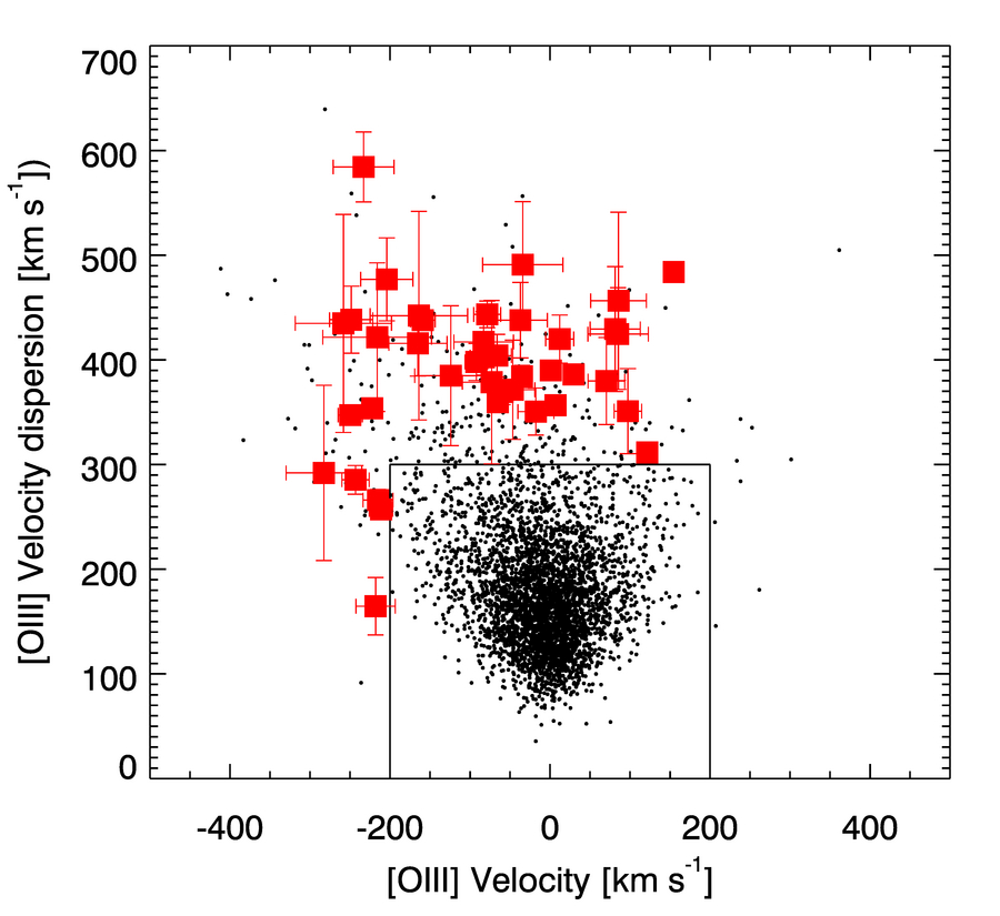
Figure 1.— [O iii] velocity versus velocity dispersion (VVD) diagram of the sample of 40 AGNs observed with SNIFS (red circles). The [O iii] velocity and velocity dispersion of these AGNs are measured from the SDSS spectra. The selection criteria of these targets are indicated with the solid box. The luminosity-limited sample of local AGNs are denoted with black dots (Woo et al., 2016).

Based on the archival spectra of the SDSS Data Release 7, Woo et al. (2016) uniformly selected a large sample ($\sim$ 39,000) of Type-2 AGNs at z $<$ 0.3 and studied the properties and fraction of ionized gas outflows. Using a sample of 235,922 emission line galaxies from the MPA-JHU Catalog, a parent sample of 106,971 Type-2 AGNs was identified in the BPT diagram (Baldwin et al., 1981; Veilleux & Osterbrock, 1987) based on the classification scheme by Kauffmann et al. (2003). Then, a sample of 38,948 Type-2 AGNs with well-defined emission line profiles was further selected based on two criteira, i.e., all targets were required to have a signal-to-noise ratio (S/N) $\geq$ 10 in the continuum, and with S/N $\geq$ 3 in the H$\beta$, [O iii]$\lambda$5007, H$\alpha$, and [N ii]$\lambda$6584 emission lines, and the amplitude-to-noise (A/N) ratios were also required to be larger than 5 for the [O iii]$\lambda$5007 and H$\alpha$ emission lines. Note that AGNs with a very weak [O iii] line are not included in this sample, suggesting that the sample is biased against low-luminosity AGNs.

We started our target selection from this sample for follow-up observations. Our selection criteria are listed as below. First, we limited the extinction-corrected [O iii] luminosity as $L_{\mathrm{\mbox{[O\,{iii}]};cor}}>10^{41.5}$ erg s^-1 and set a redshift cut of z $<0.1$, which provide us a sample of luminous AGNs to perform spatially-resolved studies of the gas kinematic in the NLRs. Woo et al. (2016) adopted the Balmer decrement (i.e., the H$\alpha$-to-H$\beta$ flux ratio of 2.86; Netzer, 2009) to correct for the extinction of [O iii] luminosity. In this case, the [O iii] luminosity increases by an average factor of $\sim$ 7 and the $L_{\mathrm{\mbox{[O\,{iii}]};cor}}>10^{41.5}$ erg s^-1 is corresponding to $L_{\mathrm{\mbox{[O\,{iii}]}}}>10^{40.7}$ erg s^-1. Following our previous studies (Karouzos et al., 2016a, b; Bae et al., 2017; Kang & Woo, 2018), we adopted the velocity shift and velocity dispersion measured from the [O iii] emission line of SDSS spectra to trace the extreme kinematic signatures of ionized gas. We limited the [O iii] velocity shift $|v_{\mbox{[O\,{iii}]}}|>200$ km s^-1 (with respect to the systemic velocity) and [O iii] velocity dispersion as $\sigma_{\mbox{[O\,{iii}]}}>300$ km s^-1. The systemic velocity and stellar velocity dispersion ($\sigma_{\ast}$) were measured from stellar absorption lines in the SDSS spectrum (Woo et al., 2016). We finally selected 40 objects out of 902 Type-2 AGNs, which satisfy the selection criteria and the visibility of SNIFS. Note that our previous GMOS studies (Karouzos et al., 2016a, b; Kang & Woo, 2018) focused on the AGNs with stronger outflow signatures (e.g., $\sigma_{\mbox{[O\,{iii}]}}>400$ km s^-1 and/or $L_{\mathrm{\mbox{[O\,{iii}]};cor}}>10^{42}$ erg s^-1).

As shown in Table 1, our SNIFS sample is dominated by spirals (21 objects) and ellipticals (12 objects) while the number of galaxies with merger or tidal features is five. Based on the comparison of larger samples of AGNs with and without outflow signatures, Luo et al. (2019) find that the presence of outflows may depend on the gas fraction in the host galaxies. Since the SNIFS sample focuses on the AGNs with strong outflow signatures, the gas fraction of their host galaxies could be different from those of the AGNs without outflow signatures. In addition, since the SNIFS sample is relatively small, it is difficult to directly compare with the un-biased sample of the hard X-ray selected AGNs, which have a higher fraction of spiral/merger morphologies in their massive host galaxies (Koss et al., 2010, 2011).

The properties of the selected AGNs measured from the integrated SDSS spectra are presented in Table 1. As shown in Fig. 4a and 4b, the radial profiles of the ratio between [O iii] velocity dispersion and stellar velocity dispersion become clearer as the extinction-uncorrected [O iii] luminosity of these AGNs increase, thus we order them by this quantity in Table 1 as well as in the following tables and figures. In Fig. 1, we present the [O iii] velocity-velocity dispersion (VVD) diagram of the total luminosity-limited sample of the SDSS AGNs.

2.2. Observations

We used the SuperNova Integral Field Spectrograph (SNIFS) at the University of Hawaii’s 2.2 m telescope (UH88) to observe the sample. SNIFS possesses a $6\farcs 4\times 6\farcs 4$ field of view, which can cover 3-12 kpc scale at the redshifts of our targets. The field of view is subdivided into a grid of $15\times 15$ spaxels, with a spaxel scale of $\sim 0\farcs 43$ ($\sim$ 200-800 pc for our targets). The dual-channel spectrograph of SNIFS simultaneously covers the wavelength range of 3200-5200 Å and 5100-10000 Å, with the spectral resolution $R\sim 1000$ and 1300, respectively. For each target, the exposure time ranges from 1200 to 8400 seconds, which were determined based on the surface brightness of SDSS images. The observations were carried out under stable weather conditions (low wind, moderate humidity, and pressure values) in four observing runs in 2014 and 2015. The seeing values varied from $0\farcs 9$ to $2\farcs 1$ with a median of $1\farcs 2$, corresponding to sub-kpc or kpc scale spatial resolution. The observation details are summarised in Table 2.

Table 2Observational log of the tagets

ID	$\alpha_{2000}$	$\delta_{2000}$	z	Obs. Date	$t_{exp}$	Seeing
	[hh mm ss.ss]	[dd mm ss.ss]			[sec]	[″]
(1)	(2)	(3)	(4)	(5)	(6)	(7)
J1042+1808	10 42 22.36	+18 08 06.72	0.0518	2015 Apr. 11	6000	1.1
J1106+4530	11 06 23.94	+45 30 39.96	0.0635	2015 Apr. 12	6000	1.2
J0952+1937	09 52 59.03	+19 37 55.41	0.0244	2015 Jan. 23	6000	1.5
J1121+2825	11 21 12.99	+28 25 10.92	0.0694	2015 Jan. 23	6000	1.8
J2328+1446	23 28 06.06	+14 46 24.96	0.0689	2014 Dec. 30	5400	1.0
J1625+2228	16 25 07.18	+22 28 53.76	0.0607	2015 Apr. 12	5400	1.0
J0758+3747	07 58 28.11	+37 47 11.84	0.0408	2014 Dec. 30	5400	1.1
J1236+1135	12 36 34.51	+11 35 34.08	0.0672	2015 Apr. 11,26	8400	1.1
J1040+3907	10 40 00.57	+39 07 19.99	0.0308	2015 Jan. 24,Apr. 25	7200	1.6
J1208+5538	12 08 18.95	+55 38 33.72	0.0513	2014 Dec. 30	5400	1.3
J1019+5857	10 19 31.71	+58 57 18.61	0.0420	2015 Jan. 25	6000	1.1
J1339+0853	13 39 15.96	+08 53 10.29	0.0662	2015 Apr. 12	6000	1.2
J0144-0110	01 44 29.17	-01 10 47.10	0.0604	2015 Jan. 24	6000	1.7
J1630+2434	16 30 02.27	+24 34 05.16	0.0619	2015 Apr. 12,13	6600	0.9
J1632+2622	16 32 33.80	+26 22 50.59	0.0587	2015 Apr. 25	5400	0.9
J1446+1122	14 46 53.53	+11 22 47.10	0.0519	2015 Apr. 26	3000	1.3
J1154+4555	11 54 36.02	+45 55 36.81	0.0431	2015 Jan. 24,Apr. 27	8400	1.3
J0130+1312	01 30 37.76	+13 12 51.99	0.0728	2015 Jan. 23,25	6000	1.2
J1301+2918	13 01 25.27	+29 18 49.43	0.0237	2015 Apr. 26	4200	1.2
J1200+0001	12 00 37.69	+00 01 26.04	0.0948	2015 Apr. 13	6000	0.9
J1443+4759	14 43 54.85	+47 59 24.36	0.0920	2015 Apr. 27	7200	1.4
J1442+2201	14 42 32.21	+22 01 16.46	0.0798	2015 Apr. 13	7200	0.9
J1520+2846	15 20 14.44	+28 46 11.28	0.0826	2015 Apr. 11	6000	1.5
J1023+1251	10 23 06.98	+12 51 00.36	0.0470	2015 Apr. 27	4800	1.0
J0836+4401	08 36 37.84	+44 01 09.58	0.0554	2015 Jan. 24,25	8400	1.3
J0753+1421	07 53 28.28	+14 21 40.97	0.0488	2015 Jan. 23	6000	1.5
J1344+5553	13 44 42.15	+55 53 13.81	0.0374	2015 Apr. 26	2400	1.3
J1550+2749	15 50 01.60	+27 49 00.48	0.0781	2015 Apr. 25	5400	0.9
J1327+1601	13 27 34.65	+16 01 11.28	0.0859	2015 Jan. 23	6000	2.1
J1037+5950	10 37 41.50	+59 50 50.02	0.0908	2015 Apr. 25	5400	1.5
J1654+1946	16 54 30.73	+19 46 15.53	0.0535	2015 Apr. 27	3600	1.4
J1532+2333	15 32 22.32	+23 33 24.98	0.0465	2015 Apr. 26	2400	1.3
J1632+2349	16 32 13.44	+23 49 09.73	0.0630	2015 Apr. 26	4800	1.3
J1540+1049	15 40 55.43	+10 49 09.48	0.0962	2015 Apr. 11,12,13	5400	1.2
J1217+0346	12 17 41.99	+03 46 31.01	0.0799	2015 Apr. 27	4800	1.0
J1018+3613	10 18 33.63	+36 13 26.40	0.0541	2014 Dec. 30	5400	1.1
J1213+5138	12 13 03.35	+51 38 54.97	0.0851	2015 Jan. 24	6000	1.7
J1434+0530	14 34 37.87	+05 30 16.16	0.0851	2015 Apr. 25	4800	0.9
J1304+3615	13 04 22.17	+36 15 43.12	0.0447	2015 Apr. 25	1200	1.5
J1147+5226	11 47 21.60	+52 26 58.78	0.0486	2015 Apr. 26	3600	1.2

Note. — Col. 1: Target ID; (2) Right ascension (J2000); (3) Declination (J2000); Col. 4: Redshift; Col. 5: Date of observation; Col. 6: Exposure time; Col. 7: Seeing size

3. Data reduction and analysis

3.1. Data reduction

All the data were pre-reduced at the observatory by using the standard pipeline for the Nearby Supernova Factory (SNfactory) project (see Aldering et al. 2006 for details). Since our targets are AGNs, we adopted a special strategy for the data reduction and started from the intermediate data products of the SNfactory pipeline. These data products were overscan and bias subtracted, flat-field and cosmic ray corrected, wavelength calibrated, and telluric feature removed. First, we adopted the IDL wrapper SLA_MOP to calculate the atmospheric differential refraction offsets and used them to recenter the data cubes. Then we masked the AGN for each data cube and measured the corresponding sky background as the average flux in the rest region of the field of view. The sky background was further subtracted from all the data cubes. During the processing of the SNfactory pipeline, all the data have been converted to units of erg s^-1 cm^-2 Å^-1. We further performed the flux calibration by matching the flux in the SDSS spectra. The red and blue spectra were calibrated separately and then combined into a uniform wavelength range of 3300-9700 Å. In order to increase the S/N, we used a 2 spaxels $\times$ 2 spaxels moving box to smooth the data and obtained the final data cube with a format of $14\times 14$ spaxels (corresponding to $6\farcs 0\times 6\farcs 0$ field of view). The smoothing scheme did not change the initial spaxel scale of the data cube. With the spaxel scale of $\sim 0\farcs 43$, we were able to Nyquist sample the seeing size (i.e. spatial resolution) and retain the spatial information of the targets.

3.2. Data analysis

We followed the method as we previously adopted (Karouzos et al., 2016a; Bae et al., 2017; Kang & Woo, 2018; Luo et al., 2019) to perform the spectral analysis, which includes the subtraction of the stellar continuum and the extraction of the ionized gas kinematics. For each spaxel, we first fitted the continuum and measure the stellar velocity shift (with respect to the systemic velocity) and velocity dispersion by using the software pPXF (Cappellari & Emsellem, 2004). In this process, the continuum was modeled with 47 MILES simple-stellar population templates, which have solar metallicity and different ages ranging from 0.63 to 12.6 Gyr (Falcón-Barroso et al., 2011). In order to determine the systemic velocity of the host galaxy, we derived the spatially integrated spectra within the central 3″ spaxels and measured the velocity shift of the stellar absorption lines in them.

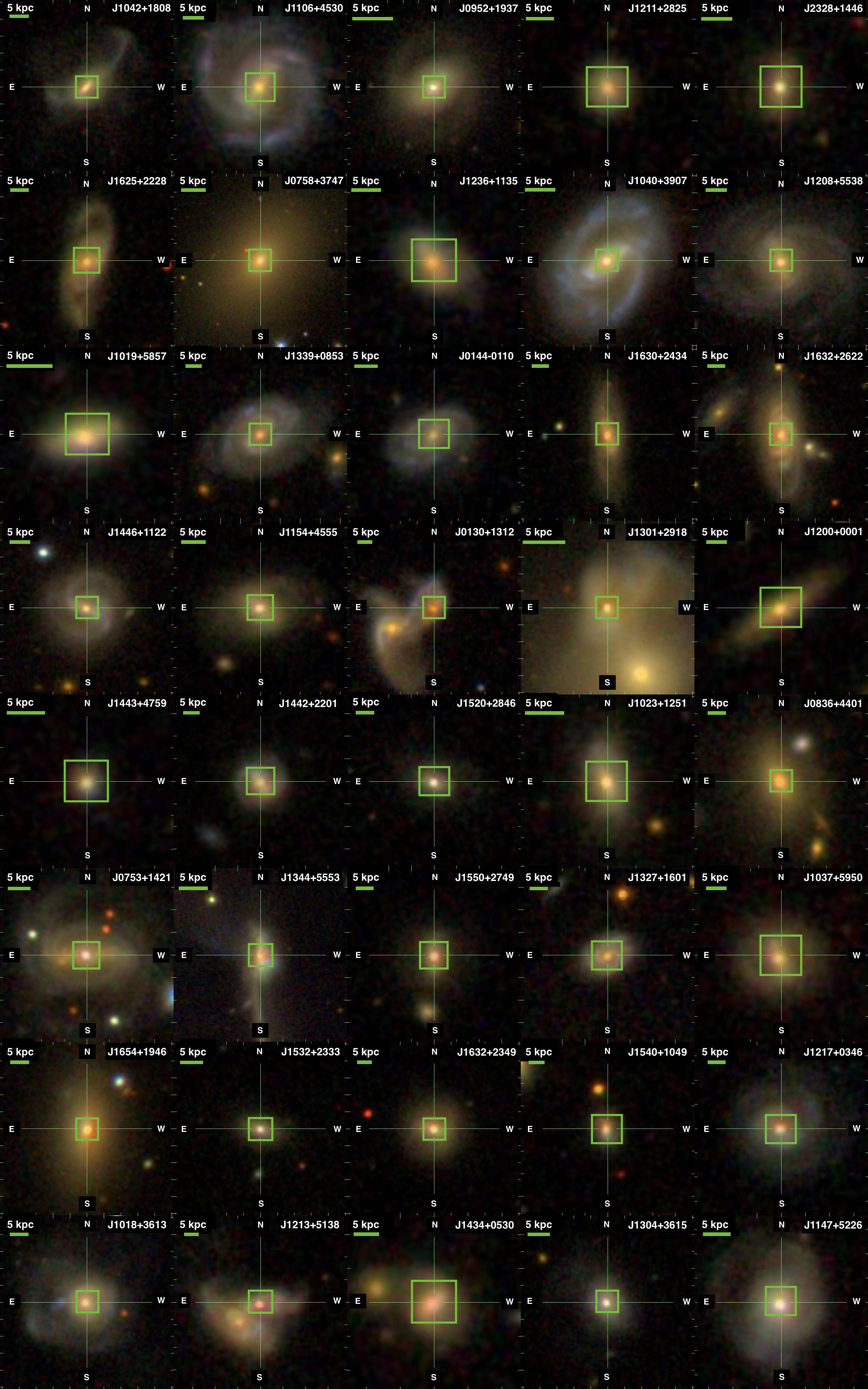
Figure 2.— SDSS gri-composite images. The field of view of SNIFS IFU ($6\farcs 4\times 6\farcs 4$) is shown with green boxes, while the horizontal green bars show 5 kpc scale.

Figure 3a.— Examples of two dimensional maps ($6\farcs 0\times 6\farcs 0$) of eight targets, from left to right column: continuum (5030 – 5170Å) flux, [O iii] flux, velocity and velocity dispersion, [O iii]/H$\beta$ flux ratio, BPT classification. The last column shows the spatially-resolved BPT diagrams ([N ii]/H$\alpha$ vs [O iii]/H$\beta$), with color-coded distance information. The horizontal white bars show 1 kpc scale. Black contours denote continuum flux levels from 10% to 90% of the peak flux in steps of 10% of the peak flux. The dotted, dashed and solid lines show the demarcation lines defined by Kewley et al. (2001), Kauffmann et al. (2003) and Cid Fernandes et al. (2010), respectively.

Figure 3b.—

Figure 4a.— Radial distributions of the ratio between [O iii] velocity dispersion and stellar velocity dispersion. The error-weighted mean (large blue circles) of $\sigma_{\mbox{[O\,{iii}]}}/\sigma_{\ast}$ in each distance bin and the measurements of each spaxel (dark gray points) are presented as a function of the radial distance. The kinematic outflow size is defined when the mean of $\sigma_{\mbox{[O\,{iii}]}}/\sigma_{\ast}$ becomes unity and equals to 1 (red solid line). The range of the outflow boundary is represented by the shaded pink region.

Figure 4b.—

For the continuum-subtracted spectra, we used the IDL procedure MPFIT (Markwardt, 2009) to fit H$\beta$, [O iii], [N ii], H$\alpha$, and [S ii] emission lines. Each line was fitted with up to two Gaussian components, including one narrow component and one broad wing component. We adopted two criteria to accept the fitting of the broad wing component: (1) Its peak amplitude is at least 2 times the continuum noise, which is determined as the standard deviation of the continuum-subtracted spectra at 5100 – 5200Å. (2) The distance between the peaks of the two Gaussian components should be smaller than the sum of their widths ($\sigma$). For the H$\alpha$+[N ii] and [S ii] regions, to reduce the freedom degrees of the fitting, we assumed the same velocity shift and velocity dispersion for the doublets ([N ii] and [S ii]), while the velocity dispersion is in turn tied to the velocity dispersion of individual H$\alpha$ components.

Based on the best-fitted line profiles, we measured the first moment $\lambda_{0}$ and second moment $\Delta\lambda^{2}$ for each emission line in each spaxel, which are defined as

$$\mathrm{\lambda_{0}}=\frac{\int\lambda f_{\lambda}d\lambda}{\int f_{\lambda}d\lambda},\;\mathrm{\Delta\lambda^{2}}=\frac{\int\lambda^{2}f_{\lambda}d\lambda}{\int f_{\lambda}d\lambda}-\mathrm{\lambda_{0}}^{2}.$$ (1)

Then we calculated the line flux, the velocity shift (with respect to the systemic velocity), and the velocity dispersion. We corrected the instrumental spectral resolution ($\sigma_{inst}\sim 110$ km s^-1) by subtracting it in quadrature from the observed velocity dispersion. In addition, we performed Monte Carlo simulations to estimate the uncertainties of the measurements. By randomizing the flux using the flux error, we produced 100 mock spectra and fitted each of them. The standard deviation of the resulting distributions was adopted as the uncertainty. An iterative 4$\sigma$ clipping algorithm was used to exclude the bad fits in this process.

Based on the above spectral analysis, we obtained the two-dimensional maps of continuum flux and emission-line flux, ionized gas velocity and velocity dispersion of each target. The continuum flux is determined as the median value of the best-fitted continuum at 5030 – 5170Å. For the [O iii] emission line, we employed an S/N limit of 3 (based on the peak S/N) to exclude spaxels with weak lines or bad measurements. Spaxels with lower S/N are masked as gray regions in the two-dimensional maps.

4. Results

In Figure 2, we present the SDSS gri-composite images of our sample and overlay the SNIFS field of view. These targets have a variety of inclinations, with the minor-to-major axis ratio ranging from 0.35 to 0.99. We collect the information of morphology classification from the Galaxy Zoo project (Lintott et al., 2011). For the targets without classification in the Galaxy Zoo project, we perform visual morphological classification based on the SDSS gri-composite images. In summary, twenty-one galaxies are classified as spiral galaxies, which show spiral arms, bars, or ring structures. Six galaxies present clear tidal or merger signatures. There are also twelve elliptical galaxies and one galaxy (J1540+1049) without clear morphology classification. The detailed morphology classifications are presented in Table 1.

4.1. Emission Line Properties

In Figure 3a and 3b, we present the two-dimensional maps of eight targets, which include the maps of continuum flux, [O iii] flux, velocity and velocity dispersion, [O iii]/H$\beta$ flux ratio, and BPT classification. The spatially resolved BPT diagrams are also shown. These targets are selected as examples of the low and high luminosity AGNs in our sample. Two-dimensional maps and spatially resolved BPT diagrams for other objects are shown in the appendix. In general, the spatial distribution of continuum flux shows a central-concentrated shape, indicating the bright nuclei of these AGNs. The [O iii] flux is less extended than the continuum flux, while it presents an equally central-concentrated shape. Note that the less-extended distribution of [O iii] flux is likely due to the observational constraints, since we require an S/N limit of 3 for the fitting of this emission line. In other words, the [O iii] region could be more extended if we consider much weak [O iii] fluxes. In the central region, the [OIII] velocity appears blue- or redshifted and the [OIII] velocity dispersion increases, both signatures of AGN-driven outflows. We use the BPT diagram to investigate the ionization mechanisms. The criteria from Kewley et al. (2001) and Kauffmann et al. (2003) are adopted to classify the AGN, composite, and star-forming regions. For dividing Seyfert and LINER regions, we use the demarcation of Cid Fernandes et al. (2010). For all the targets, the central part is classified as Seyfert and/or LINER, indicating AGN-dominated photoionization. In fifteen targets, we also find signatures of both AGN and star-formation at the outer part of the emission regions, which is shown by the BPT classification of composite and star-forming regions.

4.2. Kinematic Outflow Size

The information of spatially-resolved gas kinematics is very useful to quantify the outflow size. As shown in our previous studies (Karouzos et al., 2016a; Woo et al., 2016; Kang et al., 2017; Woo et al., 2017; Kang & Woo, 2018), the [O iii] velocity dispersion can trace the turbulent motion of ionized gas and present large values in the outflow regions. Following our previous strategy, we adopt the ratio between [O iii] and stellar velocity dispersion ($\sigma_{\mbox{[O\,{iii}]}}/\sigma_{\ast}$) to quantify the kinematic outflow size. Since $\sigma_{\ast}$ is considered as an indicator of the gravitational potential of the host galaxy, this ratio indicates the relative strength of the non-gravitational influence of AGN-driven outflows, and its radial change enables us to identify the edge of outflowing gas. The S/N of the stellar continuum of our SNIFS data is not high enough, thus we use $\sigma_{\ast}$ measured from the SDSS spectrum in the following analysis, which represents the global gravitational potential of the host galaxy. Note that the stellar velocity dispersion measured from the SDSS spectra may be overestimated due to the rotational broadening. Kang & Woo (2018) performed a consistency check to compare the stellar velocity dispersions measured from spatially-resolved GMOS spectra and those from the integrated spectra for 9 Type-2 AGNs. They found that the effect of rotational broadening is only a few percent.

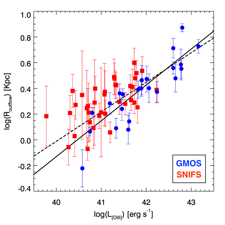
Figure 5.— Correlation between the kinematic outflow size and the [O iii] luminosity measured within the outflow size. Red points show the measurements from our sample, while blue points present the results from Kang & Woo (2018). The dashed line indicates the kinematic outflow size-luminosity relation (with the best-fitted slope of $0.230\pm 0.024$) obtained in this study, while the solid line presents the relation (with the best-fitted slope of $0.279\pm 0.035$) found in Kang & Woo (2018) for comparison.

As shown in Figure 4a and 4b, for most targets in our sample, $\sigma_{\mbox{[O\,{iii}]}}/\sigma_{\ast}$ from individual spaxels presents clearly a radial decrease and becomes unity at a large radial distance. This signature indicates that the ionized gas in the central region shows a strong non-gravitational component, while this effect becomes weak in the outer region of galaxies. To further quantify the radial behavior of the outflow kinematics, we define ten radial distance bins for each target and calculate the error-weighted mean of $\sigma_{\mbox{[O\,{iii}]}}/\sigma_{\ast}$ in each bin. The kinematic outflow size is then determined when the mean of $\sigma_{\mbox{[O\,{iii}]}}/\sigma_{\ast}$ becomes unity and equals to 1 (i.e. $\sigma_{\mbox{[O\,{iii}]}}$ becomes comparable to $\sigma_{\ast}$). We also perform a seeing correction by subtracting the half-width-at-half-maximum of seeing from the kinematic outflow size in quadrature, which is 3% on average. Considering the uncertainty of $\sigma_{\ast}$, we obtain the boundary of $\sigma_{\mbox{[O\,{iii}]}}/\sigma_{\ast}=1$ as well as the boundary of the kinematic outflow size. Note that the 2D velocity dispersion map typically shows asymmetric distribution, thus the average value in each radial bin has significant uncertainty. However, we tried to quantify a general trend as a function of radial distance. The range of this size boundary is adopted as 1$\sigma$ uncertainty of the kinematic outflow size. We exclude three targets (J0130+1312, J1042+1808, and J1208+5538) without a clear radial decrease of $\sigma_{\mbox{[O\,{iii}]}}/\sigma_{\ast}$ and measure the kinematic outflow size for 37 AGNs, which ranges from 0.9 to 4 kpc with a median value of 2 kpc (see Table 3 for details).

Table 3Host galaxy and outflow properties

ID	sSFR	Dn(4000)	H$\delta_{A}$	M${}_{\mbox{HI}}$/M∗	$\log(\mbox{M}_{\ast})$	$\sigma_{\ast}$	$\log(\mbox{L}_{\mbox{[O\,{iii}]}})$	$\log(\mbox{V}_{bulk}/\mbox{M}_{\ast})$	$\log(\mbox{V}_{bulk}/\sigma_{\ast})$	Sizeout
	[yr-1]				[M⊙]	[km s-1]	[erg s-1]			[kpc]
(1)	(2)	(3)	(4)	(5)	(6)	(7)	(8)	(9)	(10)	(11)
J1042+1808	-9.87	1.48	3.26	…	10.78	146.15	…	…	…	…
J1106+4530	-10.45	1.65	1.70	0.067	11.03	127.58	39.78	0.95	0.63	1.53$\pm$0.82
J0952+1937	…	1.16	4.30	0.135	10.38	127.09	40.83	1.46	0.66	1.24$\pm$0.46
J1121+2825	-9.60	1.47	2.45	0.042	10.32	97.980	40.43	1.39	0.73	1.87$\pm$0.48
J2328+1446	-9.97	1.40	4.22	0.091	10.15	72.480	40.36	1.36	0.81	2.40$\pm$0.72
J1625+2228	-10.32	1.67	0.50	0.037	11.04	161.13	40.31	0.87	0.49	1.62$\pm$0.50
J0758+3747	…	1.81	-0.96	0.031	11.62	263.22	40.41	0.78	0.38	1.07$\pm$0.39
J1236+1135	-9.73	1.47	1.18	0.097	10.45	97.690	40.86	1.33	0.75	2.50$\pm$0.56
J1040+3907	…	1.45	1.00	0.141	10.86	156.51	40.27	1.04	0.54	0.88$\pm$0.28
J1208+5538	-10.58	1.81	-1.28	0.047	11.07	147.44	…	…	…	…
J1019+5857	-10.03	1.49	2.23	0.083	10.35	129.98	40.75	1.39	0.62	1.37$\pm$0.46
J1339+0853	-9.62	1.48	2.79	0.127	10.77	141.94	40.70	1.02	0.55	1.83$\pm$0.58
J0144-0110	…	1.59	1.07	0.229	10.24	80.730	41.07	1.53	0.84	2.25$\pm$1.25
J1630+2434	-10.31	1.56	1.81	0.032	11.09	175.11	40.85	0.80	0.43	1.95$\pm$1.49
J1632+2622	-10.26	1.54	1.32	0.050	11.20	177.04	40.72	0.67	0.38	1.63$\pm$0.86
J1446+1122	-10.06	1.49	1.25	0.102	10.76	111.70	41.08	0.98	0.63	2.36$\pm$0.89
J1154+4555	-10.07	1.33	3.35	0.088	10.53	129.81	40.96	1.19	0.59	1.54$\pm$0.35
J0130+1312	-9.92	1.50	3.17	0.006	10.91	239.86	…	…	…	…
J1301+2918	…	1.21	2.72	0.032	10.70	174.44	41.20	0.94	0.40	1.14$\pm$0.21
J1200+0001	-10.42	1.63	1.00	0.017	10.98	170.70	40.57	0.64	0.32	2.23$\pm$1.77
J1443+4759	-9.32	1.35	7.11	…	10.10	155.10	40.68	1.43	0.49	1.76$\pm$1.19
J1442+2201	-9.76	1.32	2.39	0.139	10.60	100.60	41.29	1.12	0.69	3.08$\pm$0.98
J1520+2846	-9.77	1.26	3.93	0.345	10.44	159.35	41.29	1.38	0.55	3.00$\pm$0.83
J1023+1251	-10.27	1.57	-0.36	0.121	10.46	129.05	41.09	1.02	0.51	1.60$\pm$0.38
J0836+4401	…	2.00	-2.47	0.011	11.08	219.66	41.00	0.87	0.37	1.64$\pm$1.30
J0753+1421	-9.47	1.14	3.67	0.060	10.85	131.78	41.40	1.23	0.68	1.98$\pm$0.46
J1344+5553	…	1.25	4.38	0.134	10.86	215.03	40.70	0.89	0.33	0.85$\pm$0.17
J1550+2749	-9.50	1.33	2.11	0.045	10.68	111.44	41.33	0.96	0.61	2.66$\pm$0.62
J1327+1601	-10.16	1.51	0.83	…	10.78	131.11	41.76	1.24	0.67	3.01$\pm$0.71
J1037+5950	-9.70	1.40	3.10	0.041	10.88	130.79	41.31	0.79	0.50	2.68$\pm$0.66
J1654+1946	-10.87	1.75	-1.50	0.030	11.28	188.94	41.53	0.71	0.40	1.91$\pm$0.38
J1532+2333	-10.09	1.35	1.66	0.247	10.07	116.69	41.66	1.37	0.59	2.04$\pm$0.38
J1632+2349	-9.96	1.59	1.06	0.057	10.81	124.67	41.65	0.97	0.59	2.62$\pm$0.52
J1540+1049	-9.19	1.30	3.82	…	10.58	144.87	41.73	1.18	0.56	3.98$\pm$1.04
J1217+0346	-9.83	1.24	3.41	0.136	10.76	110.86	41.78	1.12	0.69	3.30$\pm$0.75
J1018+3613	…	1.44	2.80	0.084	10.91	183.65	41.74	1.14	0.52	1.95$\pm$0.39
J1213+5138	-9.23	1.18	3.06	…	10.91	195.21	41.69	1.06	0.46	2.58$\pm$0.82
J1434+0530	-9.28	1.25	4.53	0.041	10.90	144.05	41.91	1.06	0.59	3.44$\pm$0.86
J1304+3615	-9.03	1.20	3.84	0.268	10.39	137.46	41.81	1.50	0.63	1.79$\pm$0.50
J1147+5226	-9.61	1.24	4.75	0.310	10.69	142.94	42.23	1.03	0.53	2.45$\pm$0.57

Note. — Col. 1: Target ID; Col. 2: Specific star formation rate; Col. 3: D_n(4000); Col. 4: H$\delta_{A}$; Col. 5: HI gas fraction; Col. 6: Stellar mass; Col. 7: Stellar velocity dispersion; Col. 8 Extinction-uncorrected [O iii] luminosity measured within the outflow size: Col. 9: Bulk velocity normalized by stellar mass; Col. 10: Bulk velocity normalized by stellar velocity dispersion; Col. 11: Seeing-corrected outflow size

5. Discussion

5.1. Relation between Outflow Size and AGN Parameters

In order to understand the driving mechanism of the outflows, we examine the relation between outflow properties and AGN parameters. We first compare the kinematic outflow size with the [O iii] luminosity measured within the outflow boundary to be consistent with our previous studies performed (Karouzos et al., 2016a; Bae et al., 2017; Kang & Woo, 2018). As shown in Figure 5, the kinematic outflow size is well correlated with the [O iii] luminosity, as reported by Kang & Woo (2018). Based on the GMOS observation of 23 Type-2 AGNs over 3 orders of magnitude in [O iii] luminosity, Kang & Woo (2018) has presented the kinematic outflow size-luminosity relation with the best-fit slope of $0.279\pm 0.035$. By combining their sample with our size measurements, we can now extend the correlation with a large sample of 60 Type-2 AGNs over a broad [O iii] luminosity range. We perform a forward regression using the MPFITEXY routine (Williams et al., 2010) and obtain the best-fit relation:

$$\rm log(\frac{R_{\mathrm{out}}}{\mathrm{Kpc}})=(0.230\pm 0.024)\times\rm log(\frac{L_{\mathrm{\mbox{[O\,{iii}]}}}}{10^{42}\mathrm{ergs}^{-1}})+(0.448\pm 0.020).$$ (2)

This relation is generally consistent with that obtained by Kang & Woo (2018), which has a slightly higher slope with a smaller sample. We also compared the kinetic outflow size with black hole mass and Eddington ratio. However, we find no significant correlation. The correlation between the kinematic outflow size and [O iii] luminosity indicates that the AGNs with higher luminosity produce outflows in a larger scale, leading to more significant influence on the global kinematics of the host galaxy.

Based on the flux distribution of the [O iii] emission line, the NLR size of AGNs has been quantified using different methods and various slopes of the NLR size-luminosity relation have been reported in the literature. (Bennert et al., 2002), Schmitt et al. (2003) and Storchi-Bergmann et al. (2018) used the HST narrow-band images to measure the maximum detectable size of emitting regions in several AGN samples and obtained the best-fit slopes of $0.52\pm 0.06$, $0.33\pm 0.04$, and $0.51\pm 0.03$, respectively. Greene et al. (2011) performed a similar analysis on the long-slit data of 15 radio-quiet obscured quasars, reporting a best-fit slope of $0.22\pm 0.04$, while Fischer et al. (2018) presented a best-fit slope of $0.42\pm 0.03$ by combining the HST STIS long-slit data of 12 Type-2 quasars and the NLR size measurements from Schmitt et al. (2003). Husemann et al. (2014) and Bae et al. (2017) used an alternative definition of the NLR size and measured the flux-weighted effective radius from the IFU data of local AGN samples, reporting best-fit slopes of $0.44\pm 0.06$ and$0.41\pm 0.02$, respectively. Other studies adopted a fixed limit of the [O iii] intrinsic surface brightness to quantify the NLR size of AGNs. From the IFU and long-slit observations of radio-quiet obscured quasars, Liu et al. (2013a) obtained a best-fit slope of the NLR size-luminosity relation as $0.25\pm 0.02$, and Hainline et al. (2013) also reported a consistent result. The slope of kinematic outflow size-luminosity relation is similar or relatively shallower than those of the NLR size-luminosity relation shown as above.

As discussed in Kang & Woo (2018), the kinematic outflow size-luminosity relation is physically different from the NLR size-luminosity relation. The measurement of outflow size is based on the kinematics properties of the ionized gas, which is traced by the spatially resolved [O iii] kinematics. While the NLR size is measured from the distribution of photoionization, which is quantified from the spatial distribution of the [O iii] emission. Both outflow and photoionization processes can transfer energy from the central AGN to the host galaxy. However, the outflow process can be affected by the gas distribution and interaction as well as the gravitational potential of the host galaxy, while the photoionization process is mainly influenced by the gas distribution. Thus, the difference of the slopes between the outflow size-luminosity relation and NLR size-luminosity relation presumably indicate that the outflow and photoionization processes have different efficiencies in transferring the AGN energy. The slop of the kinetic outflow size - luminosity relation is generally shallower than that of the photoionization size -luminosity relation, implying that the kinetic energy transfer is much less efficient due to various effects including galaxy gravitational potential, local density and distribution of ISM, and the coupling efficiency between radiation and gas. For given AGN luminosity, ionizing photon can reach out a larger scale while kinetic energy is less effectively transferred, leading to a smaller kinetic outflow size than the photoionization size. We emphasize that it is important to use a proper outflow size based on kinematical information when outflow characteristics are constrained. If the photoionization size is used as a proxy of the outflow size, outflow energetics will be overestimated. Thus, it is necessary to incorporate gas kinematics in order to properly determine outflow size and outflow energetics.

Based on the [O iii] line width and surface brightness of the high-velocity gas, Sun et al. (2017) define the kinematic disturbed region (KDR) and use it to quantify the outflow properties. They find that the measured KDR size is generally lower than the NLR size, which may also support the different efficiencies between outflow and photoionization processes in transferring the AGN energy. While they obtained a KDR size-luminosity relation with a slope of 0.6, which is steeper than that of our kinematic outflow size-luminosity relation. This could be due to the difference in analysis methods: (1) they adopt a different indicator of AGN luminosity (15$\mu m$ luminosity); (2) they defined the KDR size based on an arbitrary velocity cut of 600 km s^-1 as well as surface brightness limit, which are clearly different from our definition of the kinetic outflow size. The comparison of our results with those of Sun et al. (2017) suggests that the slope is sensitive to how the outflow size is defined. As pointed out by Harrison et al. (2018), there are various definitions of outflow size, and a caution is required to compare literature results.

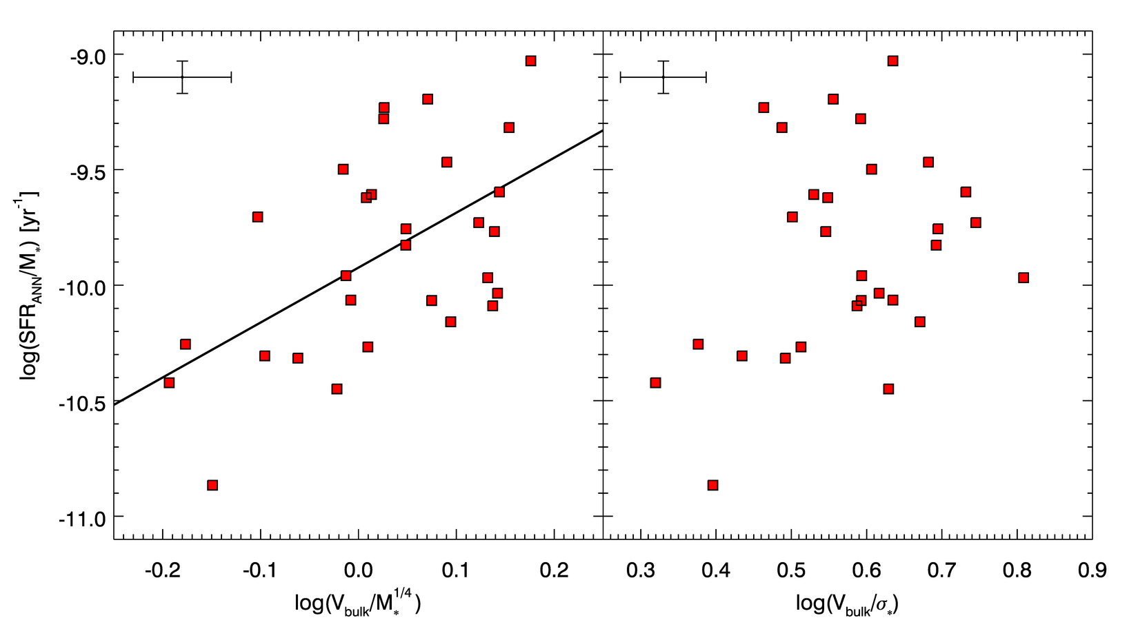
Figure 6.— Comparison of the sSFR and outflow kinematics normalized by stellar mass (left) and stellar velocity dispersion (right). The black line indicates the best-fit relation with a power-law index of 2.38. The typical error bars are shown in the upper left corners.

5.2. Relation between Outflow Kinematics and Host Galaxy Properties

We explore the feedback effect of AGN-driven outflows by comparing the outflow kinematics with the host galaxy properties, including the specific star formation rate (sSFR), D_n(4000), H${}_{\delta_{A}}$, and HI gas fraction. The direct measurement of SFR in AGN host galaxies is difficult, since the emission from AGNs contaminate the SFR tracers, i.e., the H$\alpha$ emission line, UV continuum, etc (e.g., Matsuoka & Woo 2015). We adopted the SFR from Ellison et al. (2016), which is based on artificial neural network (ANN) predictions of total infrared luminosities. Then we calculate the sSFR by dividing the SFR by stellar mass from the MPA-JHU catalog. The D_n(4000) and H${}_{\delta_{A}}$ are also adopted from the MPA-JHU catalog. The HI gas fraction can be estimated by adopting the photometric technique (e.g. Kannappan 2004; Eckert et al. 2015), which uses a broad-band color as a proxy for the cold gas mass fraction. We use the $g-i$ color from SDSS photometry for estimation and adopt the calibration by Eckert et al. (2015), as we previously applied ($log(M_{HI}/M_{*})=-0.984(2.444(g-i)+0.550(b/a))+1.881$, see for details, Luo et al. 2019). To quantify the strength of outflow kinematics, we first estimate the bulk velocity of the outflowing gas by adding the [O iii] velocity shift and dispersion of each spaxel in quadrature and calculate the flux-weighted mean within the kinematic outflow size. Then we normalize it with the stellar mass or stellar velocity dispersion which are considered as global indicators of the gravitational potential of the host galaxy. The stellar velocity dispersion is also adopted from the MPA-JHU catalog. We summarise the host galaxy and outflow properties in Table 3.

As shown in Figure 6, the sSFR of the host galaxy is positively correlated with the bulk velocity normalized by stellar mass, which indicates that AGNs with strong outflows tend to have a higher sSFR than that of the AGNs with weak outflows. The Spearman’s rank correlation coefficient is 0.5, with a p-value $<5.6\times 10^{-3}$. By removing the effect of stellar mass, the partial correlation coefficient is 0.3. The best-fitted relation between the sSFR and bulk velocity normalized by stellar mass can be quantified as a single power law with an index of 2.38. While for the bulk velocity normalized by the stellar velocity dispersion, we can not find a clear correlation with the sSFR of the host galaxy. Although the correlation is not strong, it seems that there is a broad trend between sSFR and the normalized bulk velocity by stellar velocity dispersion. Since stellar velocity dispersion suffers various effects, including inclination to the line-of-sight, and aperture size, stellar mass may better represent the host galaxy gravitational potential in normalizing gas bulk velocity. In Figure 7, we compare our AGN sample with large samples of star-forming galaxies and AGNs in the diagram of sSFR versus stellar mass. The large samples of star-forming galaxies and AGNs are adopted from (Woo et al., 2017), which are selected from the emission line galaxies at z $<$ 0.3, based on the archival spectra of the SDSS Data Release 7. The solid line indicates the median log(sSFR) of the star-forming galaxies in the main sequence. The AGNs with strong outflows have comparable sSFR as the star-forming galaxies in the main sequence, while the average sSFR of the AGNs with weak outflows is one dex lower. We also present the diagram of D_n(4000) versus H${}_{\delta_{A}}$ in Figure 8, which is color-coded by the normalized bulk velocity of the outflowing gas. The AGNs with strong outflows have relatively lower D_n(4000) and higher H${}_{\delta_{A}}$ than those with weak outflows. Since D_n(4000) and H${}_{\delta_{A}}$ are indicators of SFR, this result implies more intensive star formation in the host galaxies of AGNs with strong outflows, in agreement with the above results obtained from the IR-based SFR.

The relations between outflow kinematics and star formation are generally consistent with our previous statistical study of outflow impact in a large sample of Type-1 and Type-2 AGNs (Woo et al., 2017, 2020), which showed that star formation rate is higher for strong outflow AGNs, suggesting no instantaneous suppression or quenching of star formation while the effect of feedback is delayed. When the AGNs and star formation are triggered by enough gas supply, the AGNs are strong and can produce strong outflows, while the star formation is on-going as in regular star forming galaxies. If the outflows can only impact the ISM after a certain timescale, although the feedback effect can be observed as the SFR decrease, the AGNs will also become weak and only show weak outflows. While our study focus on AGNs in the local universe, several studies have also shown that AGNs at higher redshift (e.g. z$\sim$2 ) do not have instantaneous impact on the star formation in the host galaxies (Harrison, 2017). Scholtz et al. (2020) examine the spatial anti-correlation between the AGN-driven outflows and in-situ star formation in eight moderate-luminosity AGNs at z$=$1.4–2.6. In three targets with significant outflow signatures, they can not find a clear evidence that outflows suppress the star formation. Davies et al. (2020) find powerfull AGN-driven outflows ($V_{out}\sim$ 1500 km s^-1) in two compact star forming galaxies at z$=$2.2, which are located at the upper envelope of the star-forming main sequence, suggesting no instantaneous feedback effect of AGN in these galaxies.

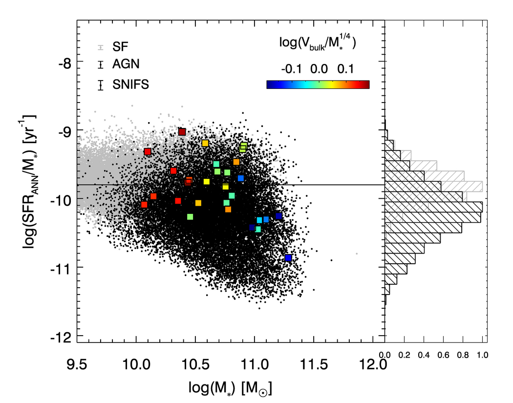
Figure 7.— The relation between the stellar mass and sSFR. Two large samples of star forming galaxies and AGNs at z $<$ 0.3 are shown in gray and black dots, respectively. The black horizontal line indicates the median log(sSFR) of the star forming galaxies in the main sequence. The typical error bars are shown in the upper left corner. Different colors represent the outflow kinematics normalized by stellar mass.

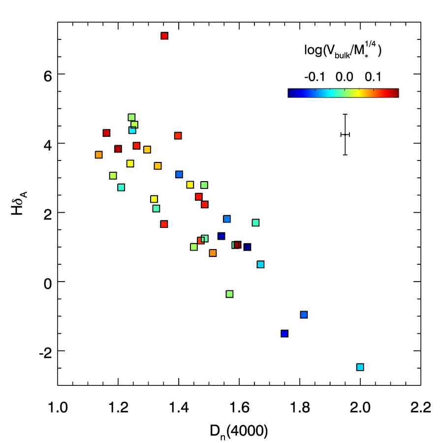
Figure 8.— The D_n(4000) vs. H$\delta_{A}$ plane. The typical error bars are shown in the upper right corner. Different colors represent the outflow kinematics normalized by stellar mass.

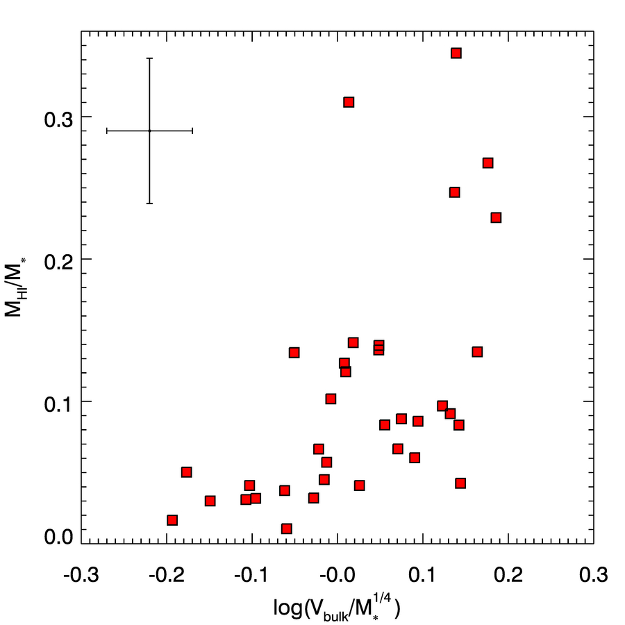
Figure 9.— Comparison of the HI gas fraction and outflow kinematics normalized by stellar mass. The typical error bars are shown in the upper left corner.

As discussed in Woo et al. (2017, 2020), the aforementioned link between AGN outflows and sSFR can also be explained as a natural consequence of gas fraction decreasing due to the internal or external mechanisms. When there is a large amount of gas in the host galaxy, both AGN and star formation are strong, which enables us to observe the strong outflows. As the supplied gas is depleted, the AGN activity and star formation will decrease, and we can only observe the weak outflows in the host galaxies with lower SFR. In addition, it is also possible that the gas fraction is intrinsically different among the host galaxies. We examine the relation between the strength of outflow kinematics and HI gas fraction in Figure 9. For the AGNs with strong outflows, the HI gas fraction tends to increase with the normalized bulk velocity and can reach the  relatively high value of 0.3, while the HI gas fraction is on average lower in the AGNs with weak outflows and does not vary with the normalized bulk velocity. This result indicates the importance of cold gas content in understanding the relation between AGN-driven outflows and sSFR. Since we can not trace the time evolution of the intrinsic gas fraction, it is difficult to test the above scenarios. Cosmological simulations like IllustrisTNG may help to investigate the time evolution of the gas content in the host galaxies of AGNs and provide hints on the exact scenario. The relation between HI gas fraction and normalized bulk velocity also suggests that the presence of outflows may depend on the gas fraction, which has been discussed in Luo et al. (2019) based on a large sample of AGNs with and without outflow. As the HI gas fraction is estimated indirectly, multiwavelength follow-up observations will provide better constraints on the intrinsic gas fraction and enable us to further study the connection between cold gas, star formation, and AGN outflows.

6. Summary

To investigate the feedback effect of AGN-driven outflows, we perform integral-field spectroscopic observations of 40 moderate-luminosity ($10^{41.5}<L_{\mathrm{\mbox{[O\,{iii}]};cor}}<10^{43.1}$ erg s^-1 ) Type-2 AGNs at z $<$ 0.1. These targets are selected from the a large sample of $\sim$39,000 Type-2 AGNs based on their integrated [O iii] kinematics, which provide us a uniform sample to quantify the outflow properties and compare them with the properties of AGN and host galaxy. We summarize the main results as below.

• Based on the radial profile of the normalized [O iii] velocity dispersion by stellar velocity dispersion, we measure the kinematic outflow size, which ranges from 0.9 to 4 kpc with a median value of 2 kpc. By including the size measurements from Kang & Woo (2018), we confirm that the kinematic outflow size is well correlated with the [O iii] luminosity. The slope of the best-fitted relation is $0.23\pm 0.02$, which is slightly lower than that obtained in Kang & Woo (2018). Our results further confirm the kinematic outflow size-luminosity relation reported in Kang & Woo (2018) and extend it into a broader [O iii] luminosity range (over four orders of magnitude in [O III] luminosity).

• We compare the outflow kinematics with the host galaxy properties, including the sSFR, D_n(4000), H${}_{\delta_{A}}$, and HI gas fraction. We find a clear correlation between the sSFR and normalized outflow velocity. The AGNs with strong outflows have comparable sSFR to the star-forming galaxies in the main sequence, while the AGNs with weak outflows present much lower sSFR. In addition, we also find that AGNs with strong outflows have higher star formation rate and HI gas fraction than those with weak outflows. These results are consistent with our previous studies of outflow impact in large samples of AGNs (Woo et al., 2017, 2020), suggesting that the current feedback from AGN-driven outflows do not instantaneously suppress or quench the star formation in the host galaxies while its effect is delayed.

Appendix A Additional Figures

Figure A.1.—

Figure A.2.—

Figure A.3.—

Figure A.4.—

Figure A.5.—

Figure A.6.—

Figure A.7.—

Figure A.8.—

References

- Aldering et al. (2002) Aldering, G., Adam, G., Antilogus, P., et al. 2002, in Society of Photo-Optical Instrumentation Engineers (SPIE) Conference Series, Vol. 4836, Survey and Other Telescope Technologies and Discoveries, ed. J. A. Tyson & S. Wolff, 61–72
- Aldering et al. (2006) Aldering, G., Antilogus, P., Bailey, S., et al. 2006, ApJ, 650, 510, doi: 10.1086/507020
- Bae & Woo (2014) Bae, H.-J., & Woo, J.-H. 2014, ApJ, 795, 30, doi: 10.1088/0004-637X/795/1/30
- Bae et al. (2017) Bae, H.-J., Woo, J.-H., Karouzos, M., et al. 2017, ApJ, 837, 91, doi: 10.3847/1538-4357/aa5f5c
- Baldwin et al. (1981) Baldwin, J. A., Phillips, M. M., & Terlevich, R. 1981, PASP, 93, 5, doi: 10.1086/130766
- Bennert et al. (2002) Bennert, N., Falcke, H., Schulz, H., Wilson, A. S., & Wills, B. J. 2002, ApJ, 574, L105, doi: 10.1086/342420
- Cappellari & Emsellem (2004) Cappellari, M., & Emsellem, E. 2004, PASP, 116, 138, doi: 10.1086/381875
- Carniani et al. (2015) Carniani, S., Marconi, A., Maiolino, R., et al. 2015, A&A, 580, A102, doi: 10.1051/0004-6361/201526557
- Carniani et al. (2016) —. 2016, A&A, 591, A28, doi: 10.1051/0004-6361/201528037
- Cazzoli et al. (2016) Cazzoli, S., Arribas, S., Maiolino, R., & Colina, L. 2016, A&A, 590, A125, doi: 10.1051/0004-6361/201526788
- Cicone et al. (2012) Cicone, C., Feruglio, C., Maiolino, R., et al. 2012, A&A, 543, A99, doi: 10.1051/0004-6361/201218793
- Cicone et al. (2014) Cicone, C., Maiolino, R., Sturm, E., et al. 2014, A&A, 562, A21, doi: 10.1051/0004-6361/201322464
- Cid Fernandes et al. (2010) Cid Fernandes, R., Stasińska, G., Schlickmann, M. S., et al. 2010, MNRAS, 403, 1036, doi: 10.1111/j.1365-2966.2009.16185.x
- Circosta et al. (2018) Circosta, C., Mainieri, V., Padovani, P., et al. 2018, A&A, 620, A82, doi: 10.1051/0004-6361/201833520
- Cresci et al. (2015a) Cresci, G., Mainieri, V., Brusa, M., et al. 2015a, ApJ, 799, 82, doi: 10.1088/0004-637X/799/1/82
- Cresci et al. (2015b) Cresci, G., Marconi, A., Zibetti, S., et al. 2015b, A&A, 582, A63, doi: 10.1051/0004-6361/201526581
- Davies et al. (2014) Davies, R. I., Maciejewski, W., Hicks, E. K. S., et al. 2014, ApJ, 792, 101, doi: 10.1088/0004-637X/792/2/101
- Davies et al. (2020) Davies, R. L., Förster Schreiber, N. M., Lutz, D., et al. 2020, ApJ, 894, 28, doi: 10.3847/1538-4357/ab86ad
- Eckert et al. (2015) Eckert, K. D., Kannappan, S. J., Stark, D. V., et al. 2015, ApJ, 810, 166, doi: 10.1088/0004-637X/810/2/166
- Ellison et al. (2016) Ellison, S. L., Teimoorinia, H., Rosario, D. J., & Mendel, J. T. 2016, MNRAS, 458, L34, doi: 10.1093/mnrasl/slw012
- Elvis (2000) Elvis, M. 2000, ApJ, 545, 63, doi: 10.1086/317778
- Fabian (2012) Fabian, A. C. 2012, ARA&A, 50, 455, doi: 10.1146/annurev-astro-081811-125521
- Falcón-Barroso et al. (2011) Falcón-Barroso, J., Sánchez-Blázquez, P., Vazdekis, A., et al. 2011, A&A, 532, A95, doi: 10.1051/0004-6361/201116842
- Feruglio et al. (2010) Feruglio, C., Maiolino, R., Piconcelli, E., et al. 2010, A&A, 518, L155, doi: 10.1051/0004-6361/201015164
- Fiore et al. (2017) Fiore, F., Feruglio, C., Shankar, F., et al. 2017, A&A, 601, A143, doi: 10.1051/0004-6361/201629478
- Fischer et al. (2018) Fischer, T. C., Kraemer, S. B., Schmitt, H. R., et al. 2018, ApJ, 856, 102, doi: 10.3847/1538-4357/aab03e
- Fluetsch et al. (2019) Fluetsch, A., Maiolino, R., Carniani, S., et al. 2019, MNRAS, 483, 4586, doi: 10.1093/mnras/sty3449
- Förster Schreiber et al. (2019) Förster Schreiber, N. M., Übler, H., Davies, R. L., et al. 2019, ApJ, 875, 21, doi: 10.3847/1538-4357/ab0ca2
- Freitas et al. (2018) Freitas, I. C., Riffel, R. A., Storchi-Bergmann, T., et al. 2018, MNRAS, 476, 2760, doi: 10.1093/mnras/sty303
- García-Burillo et al. (2015) García-Burillo, S., Combes, F., Usero, A., et al. 2015, A&A, 580, A35, doi: 10.1051/0004-6361/201526133
- Genzel et al. (2014) Genzel, R., Förster Schreiber, N. M., Rosario, D., et al. 2014, ApJ, 796, 7, doi: 10.1088/0004-637X/796/1/7
- Greene et al. (2011) Greene, J. E., Zakamska, N. L., Ho, L. C., & Barth, A. J. 2011, ApJ, 732, 9, doi: 10.1088/0004-637X/732/1/9
- Hainline et al. (2013) Hainline, K. N., Hickox, R., Greene, J. E., Myers, A. D., & Zakamska, N. L. 2013, ApJ, 774, 145, doi: 10.1088/0004-637X/774/2/145
- Harrison (2017) Harrison, C. M. 2017, Nature Astronomy, 1, 0165, doi: 10.1038/s41550-017-0165
- Harrison et al. (2014) Harrison, C. M., Alexander, D. M., Mullaney, J. R., & Swinbank, A. M. 2014, MNRAS, 441, 3306, doi: 10.1093/mnras/stu515
- Harrison et al. (2018) Harrison, C. M., Costa, T., Tadhunter, C. N., et al. 2018, Nature Astronomy, 2, 198, doi: 10.1038/s41550-018-0403-6
- Harrison et al. (2012) Harrison, C. M., Alexander, D. M., Mullaney, J. R., et al. 2012, ApJ, 760, L15, doi: 10.1088/2041-8205/760/1/L15
- Harrison et al. (2016) —. 2016, MNRAS, 456, 1195, doi: 10.1093/mnras/stv2727
- Heckman & Best (2014) Heckman, T. M., & Best, P. N. 2014, ARA&A, 52, 589, doi: 10.1146/annurev-astro-081913-035722
- Husemann et al. (2014) Husemann, B., Jahnke, K., Sánchez, S. F., et al. 2014, MNRAS, 443, 755, doi: 10.1093/mnras/stu1167
- Husemann et al. (2016) Husemann, B., Scharwächter, J., Bennert, V. N., et al. 2016, A&A, 594, A44, doi: 10.1051/0004-6361/201527992
- Husemann et al. (2019) Husemann, B., Bennert, V. N., Jahnke, K., et al. 2019, ApJ, 879, 75, doi: 10.3847/1538-4357/ab24bc
- Kang & Woo (2018) Kang, D., & Woo, J.-H. 2018, ApJ, 864, 124, doi: 10.3847/1538-4357/aad561
- Kang et al. (2017) Kang, D., Woo, J.-H., & Bae, H.-J. 2017, ApJ, 845, 131, doi: 10.3847/1538-4357/aa80e8
- Kannappan (2004) Kannappan, S. J. 2004, ApJ, 611, L89, doi: 10.1086/423785
- Karouzos et al. (2016a) Karouzos, M., Woo, J.-H., & Bae, H.-J. 2016a, ApJ, 819, 148, doi: 10.3847/0004-637X/819/2/148
- Karouzos et al. (2016b) —. 2016b, ApJ, 833, 171, doi: 10.3847/1538-4357/833/2/171
- Kauffmann et al. (2003) Kauffmann, G., Heckman, T. M., Tremonti, C., et al. 2003, MNRAS, 346, 1055, doi: 10.1111/j.1365-2966.2003.07154.x
- Kewley et al. (2001) Kewley, L. J., Dopita, M. A., Sutherland, R. S., Heisler, C. A., & Trevena, J. 2001, ApJ, 556, 121, doi: 10.1086/321545
- Koss et al. (2010) Koss, M., Mushotzky, R., Veilleux, S., & Winter, L. 2010, ApJ, 716, L125, doi: 10.1088/2041-8205/716/2/L125
- Koss et al. (2011) Koss, M., Mushotzky, R., Veilleux, S., et al. 2011, ApJ, 739, 57, doi: 10.1088/0004-637X/739/2/57
- Lantz et al. (2004) Lantz, B., Aldering, G., Antilogus, P., et al. 2004, in Society of Photo-Optical Instrumentation Engineers (SPIE) Conference Series, Vol. 5249, Optical Design and Engineering, ed. L. Mazuray, P. J. Rogers, & R. Wartmann, 146–155
- Leung et al. (2019) Leung, G. C. K., Coil, A. L., Aird, J., et al. 2019, ApJ, 886, 11, doi: 10.3847/1538-4357/ab4a7c
- Lintott et al. (2011) Lintott, C., Schawinski, K., Bamford, S., et al. 2011, MNRAS, 410, 166, doi: 10.1111/j.1365-2966.2010.17432.x
- Liu et al. (2013a) Liu, G., Zakamska, N. L., Greene, J. E., Nesvadba, N. P. H., & Liu, X. 2013a, MNRAS, 436, 2576, doi: 10.1093/mnras/stt1755
- Liu et al. (2013b) —. 2013b, MNRAS, 430, 2327, doi: 10.1093/mnras/stt051
- Luo et al. (2019) Luo, R., Woo, J.-H., Shin, J., et al. 2019, ApJ, 874, 99, doi: 10.3847/1538-4357/ab08e6
- Maiolino et al. (2012) Maiolino, R., Gallerani, S., Neri, R., et al. 2012, MNRAS, 425, L66, doi: 10.1111/j.1745-3933.2012.01303.x
- Maiolino et al. (2017) Maiolino, R., Russell, H. R., Fabian, A. C., et al. 2017, Nature, 544, 202, doi: 10.1038/nature21677
- Markwardt (2009) Markwardt, C. B. 2009, in Astronomical Society of the Pacific Conference Series, Vol. 411, Astronomical Data Analysis Software and Systems XVIII, ed. D. A. Bohlender, D. Durand, & P. Dowler, 251
- Matsuoka & Woo (2015) Matsuoka, K., & Woo, J.-H. 2015, ApJ, 807, 28, doi: 10.1088/0004-637X/807/1/28
- McElroy et al. (2015) McElroy, R., Croom, S. M., Pracy, M., et al. 2015, MNRAS, 446, 2186, doi: 10.1093/mnras/stu2224
- Mullaney et al. (2013) Mullaney, J. R., Alexander, D. M., Fine, S., et al. 2013, MNRAS, 433, 622, doi: 10.1093/mnras/stt751
- Nesvadba et al. (2008) Nesvadba, N. P. H., Lehnert, M. D., De Breuck, C., Gilbert, A. M., & van Breugel, W. 2008, A&A, 491, 407, doi: 10.1051/0004-6361:200810346
- Netzer (2009) Netzer, H. 2009, MNRAS, 399, 1907, doi: 10.1111/j.1365-2966.2009.15434.x
- Rakshit & Woo (2018) Rakshit, S., & Woo, J.-H. 2018, ApJ, 865, 5, doi: 10.3847/1538-4357/aad9f8
- Revalski et al. (2018) Revalski, M., Crenshaw, D. M., Kraemer, S. B., et al. 2018, ApJ, 856, 46, doi: 10.3847/1538-4357/aab107
- Rupke et al. (2017) Rupke, D. S. N., Gültekin, K., & Veilleux, S. 2017, ApJ, 850, 40, doi: 10.3847/1538-4357/aa94d1
- Rupke & Veilleux (2013) Rupke, D. S. N., & Veilleux, S. 2013, ApJ, 768, 75, doi: 10.1088/0004-637X/768/1/75
- Schmitt et al. (2003) Schmitt, H. R., Donley, J. L., Antonucci, R. R. J., et al. 2003, ApJ, 597, 768, doi: 10.1086/381224
- Scholtz et al. (2020) Scholtz, J., Harrison, C. M., Rosario, D. J., et al. 2020, MNRAS, 492, 3194, doi: 10.1093/mnras/staa030
- Sharp & Bland-Hawthorn (2010) Sharp, R. G., & Bland-Hawthorn, J. 2010, ApJ, 711, 818, doi: 10.1088/0004-637X/711/2/818
- Shin et al. (2019) Shin, J., Woo, J.-H., Chung, A., et al. 2019, ApJ, 881, 147, doi: 10.3847/1538-4357/ab2e72
- Storchi-Bergmann et al. (2010) Storchi-Bergmann, T., Lopes, R. D. S., McGregor, P. J., et al. 2010, MNRAS, 402, 819, doi: 10.1111/j.1365-2966.2009.15962.x
- Storchi-Bergmann et al. (2018) Storchi-Bergmann, T., Dall’Agnol de Oliveira, B., Longo Micchi, L. F., et al. 2018, ApJ, 868, 14, doi: 10.3847/1538-4357/aae7cd
- Sun et al. (2017) Sun, A.-L., Greene, J. E., & Zakamska, N. L. 2017, ApJ, 835, 222, doi: 10.3847/1538-4357/835/2/222
- Veilleux et al. (2005) Veilleux, S., Cecil, G., & Bland-Hawthorn, J. 2005, ARA&A, 43, 769, doi: 10.1146/annurev.astro.43.072103.150610
- Veilleux & Osterbrock (1987) Veilleux, S., & Osterbrock, D. E. 1987, ApJS, 63, 295, doi: 10.1086/191166
- Venturi et al. (2018) Venturi, G., Nardini, E., Marconi, A., et al. 2018, A&A, 619, A74, doi: 10.1051/0004-6361/201833668
- Wallace (1994) Wallace, P. T. 1994, in Astronomical Society of the Pacific Conference Series, Vol. 61, Astronomical Data Analysis Software and Systems III, ed. D. R. Crabtree, R. J. Hanisch, & J. Barnes, 481
- Wallace (2014) Wallace, P. T. 2014, SLALIB: A Positional Astronomy Library. http://ascl.net/1403.025
- Wang et al. (2011) Wang, J., Mao, Y. F., & Wei, J. Y. 2011, ApJ, 741, 50, doi: 10.1088/0004-637X/741/1/50
- Wang et al. (2018) Wang, J., Xu, D. W., & Wei, J. Y. 2018, ApJ, 852, 26, doi: 10.3847/1538-4357/aa9d1b
- Williams et al. (2010) Williams, M. J., Bureau, M., & Cappellari, M. 2010, MNRAS, 409, 1330, doi: 10.1111/j.1365-2966.2010.17406.x
- Woo et al. (2016) Woo, J.-H., Bae, H.-J., Son, D., & Karouzos, M. 2016, ApJ, 817, 108, doi: 10.3847/0004-637X/817/2/108
- Woo et al. (2017) Woo, J.-H., Son, D., & Bae, H.-J. 2017, ApJ, 839, 120, doi: 10.3847/1538-4357/aa6894
- Woo et al. (2020) Woo, J.-H., Son, D., & Rakshit, S. 2020, ApJ, 901, 66, doi: 10.3847/1538-4357/abad97
- Zhang et al. (2011) Zhang, K., Dong, X.-B., Wang, T.-G., & Gaskell, C. M. 2011, ApJ, 737, 71, doi: 10.1088/0004-637X/737/2/71