Investigating Ground-level Ozone Formation: A Case Study in Taiwan

Abstract

Tropospheric ozone (O3) is a greenhouse gas which can absorb heat and make the weather even hotter during extreme heatwaves. Besides, it is an influential ground-level air pollutant which can severely damage the environment. Thus evaluating the importance of various factors related to the O3 formation process is essential. However, O3 simulated by the available climate models exhibits large variance in different places, indicating the insufficiency of models in explaining the O3 formation process correctly. In this paper, we aim to identify and understand the impact of various factors on O3 formation and predict the O3 concentrations under different pollution-reduced and climate change scenarios. We employ six supervised methods to estimate the observed O3 using fourteen meteorological and chemical variables. We find that the deep neural network (DNN) and long short-term memory (LSTM) based models can predict O3 concentrations accurately. We also demonstrate the importance of several variables in this prediction task. The results suggest that while Nitrogen Oxides negatively contributes to predicting O3, solar radiation makes a significantly positive contribution. Furthermore, we apply our two best models on O3 prediction under different global warming and pollution reduction scenarios to improve the policy-making decisions in the O3 reduction.

1 Introduction

Ozone (O3) plays an essential role in the stratosphere to prevent organisms in the biosphere from exposing to excessive ultraviolet (UV) rays (Seinfeld & Pandis, 2016). However, it is also a greenhouse gas and a severe air pollutant at the ground-level. Ground-level O3 can absorb longwave radiation from the earth, further shifting the radiation balance and even heating the surrounding atmosphere (Stevenson et al., 2013). High concentrations of the ground-level O3 can also severely damage the ecological community. For instance, $4-15\%$ of global wheat yields are lost because of O3 pollution (Ainsworth, 2017). Therefore, the Environmental Protection Agency (EPA) of the United States set a National Ambient Air Quality Standards (NAAQS) for six principal pollutants including ground-level O3. According to the latest 2015 NAAQS, the standard for ground-level O3 is 0.070 ppm for an eight-hour average. Considering that tropospheric O3 is produced through complicated reactions, understanding the importance of different variables and their interactions that produce O3 is necessary. However, as an obvious model-observation disparity of tropospheric O3 still exists in current global-scale chemical models developed based on theoretical studies (Young et al., 2018), analyzing its formation with new data-driven methods becomes essential.

Several popular machine learning algorithms have been applied in the real-time prediction and down-scaling of O3 concentration  (Eslami et al., 2019; Watson et al., 2019). These methods are also used to simplify the O3 prediction process in climate models and reduce the computational expense of fully interactive atmospheric chemistry schemes (Nowack et al., 2018). However, most of them focus only on the prediction task and ignore the comparison of the importance of the features with earlier theoretical studies. It is essential to understand the importance of the factors in the complex O3 formation process to help improve policy-making and progress towards a healthier environment. In this study, we predict ground-level O3 with different machine learning models and measure the importance of several factors involved in O3 formation.

The availability of enormous data such as satellite observation images and uninterrupted surface measurements helps in understanding tropospheric O3 formation. The present modern techniques (e.g., deep learning methods) are also compatible with large-scale data and highly effective in making predictions. In this paper, we utilize large scale data and modern deep learning techniques to understand O3 formation. The meteorological parameters and the concentration of pollutants are adequate for ground-level O3 prediction. We use fourteen such variables in our analysis. The observed O3 is regarded as true values for the prediction. We aim to learn a prediction function $f$ that takes these fourteen variables as input features ($\mathbb{X}$) and predict the value ($y$) of the observed O3. Our main contributions are as follows:

• We collect a large dataset on observed O3 and corresponding important weather factors. We build several supervised learning methods to accurately predict O3 concentrations.

• We demonstrate the importance of several factors (variables) in this prediction task by applying two well-known frameworks for identifying feature importance.

• We apply our two best models under different global warming and pollution reduction scenarios to improve the policy-making decisions in the O3 reduction.

2 Data and Methods

Dataset

The dataset contains $14$ variables of three different types and a total of $3,204,710$ hourly data points observed during the span of $2014-2018$. We combine consecutive eight hourly data points which does not include any missing value to generate a new 2-dimension dataset (eight hours of 14 variables). We use data observed in $2014-2017$ ($655,850$ points) and in $2018$ ($225,478$ points) for training and testing respectively. The three different types of variables are as follows. (1) The in-site measurements: These include $12$ variables measured every hour at $36$ surface stations arranged by the Environmental Protection Agency (EPA) of Taiwan, as shown in Figure 1a. (2) The derived variable: These contains water vapor mixing ratio converted from the previous EPA information. (3) The observations from remote sensor: These are the surface downward solar radiation (rsds) data inverted from the absorption data of Himawari 8, a Japan’s geostationary meteorological satellite, by the Central Weather Bureau and National Science and Technology Center for Disaster Reduction of Taiwan (Bessho et al., 2016). Table 1 presents the details of each variable. The values of these inputs (independent) variables are observed hourly.

Variable	Unit	Data source
Air temperature (T)	∘C	Taiwan EPA
Wind speed (WS)	m/s	Taiwan EPA
Wind direction (WDIR)	degree	Taiwan EPA
Relative humidity (RH)	%	Taiwan EPA
Water vapor mixing ratio ($\textrm{e}_{w}$)	g/kg	Convert from RH and T
Surface downward solar radiation (rsds)	$\textrm{W}/m^{2}$	Calculate from Himawari 8 observation
Nitric oxide (NO)	ppb	Taiwan EPA
Nitrogen dioxide (NO2)	ppb	Taiwan EPA
Carbon monoxide (CO)	ppm	Taiwan EPA
Methane (CH4)	ppm	Taiwan EPA
Non-methane Hydrocarbon (NMHC)	ppm	Taiwan EPA
Sulfur dioxide (SO2)	ppb	Taiwan EPA
$\rm PM_{2.5}$	$\rm\mu g/m^{3}$	Taiwan EPA
$\rm PM_{10}$	$\rm\mu g/m^{3}$	Taiwan EPA
Ozone (O3)	ppb	Taiwan EPA

Table 1: The variables in the dataset: Observed O3 is regarded as true values for predictions. $WS$ is measured in meter per second (m/s). $WDIR$ is recorded in degrees from 0 to 360 with 0 as north. $T$ is measured in Celsius (^∘C). The $e_{w}$ is converted to gram per kilogram air (g/kg). Trace gases are measured in either parts-per million (ppm) or parts-per billion (ppb). Particulate matters are recorded in microgram per cubic meter air ($\rm\mu g/m^{3}$).

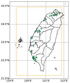
(a) EPA stations distribution

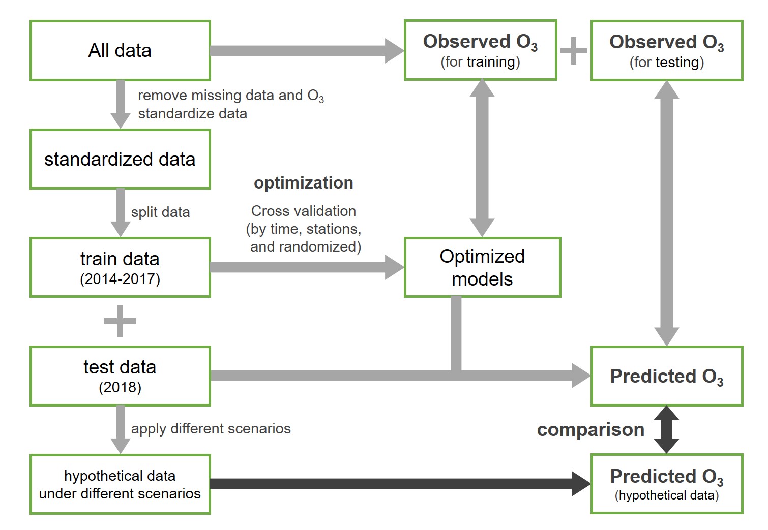
(b) Experiment procedure

Figure 1: (a) The distribution of the EPA stations in Taiwan. The orange frame is the area that we analyze from the CESM2 model, which covers most Taiwan island and outlying islands. (b) The scheme of the experiment procedures.

In addition to the observed data, monthly historical simulation (2000-2014) (Danabasoglu, 2019a) and future projection (2015-2100) (Danabasoglu, 2019b; c; d; e) from CESM2 are used to evaluate the future trend of O3. CESM2 is a global climate model developed by the US National Center for Atmospheric Research (Danabasoglu et al., 2020). The variables including temperature, relative humidity and water vapor content are analyzed in the form of an area average (longitude from 119.375 ^∘E to 121.875 ^∘E and latitude from 21.675 ^∘N to 25.445 ^∘N, as displayed in Fig. 1a).

Methods

We formulate our problem as a regression problem and use six different algorithms: linear regression (LR), random forest (RF), optimized distributed gradient boosting model (XGBoost), convolution neural network (CNN), deep neural network (DNN), and long short-term memory model (LSTM). We aim to predict the eight-hour average observed ground-level ozone. The DNN model consists of five hidden layers with 16 nodes each. The CNN model is made up of 2 convolution layers of 32 nodes with a 3x3 window, a max pooling, a flattening, and a fully-connected layer. 20% data are dropped out after the first convolution layer and the max pooling layer individually. The LSTM model consists of two LSTM layers with 25 nodes each and a fully-connected layer. The previously described consecutive 8-hour 14 variables are reshaped to the 1-dimensional input data for models including LR, RF, XGBoost, and DNN. The consecutive 8-hour 14 variables is prepared as the 2-dimension input data for the CNN and LSTM models. We describe the entire experimental setup in Figure 1b.

3 Experimental Results

We demonstrate three types of results. First, we describe the performance of all the proposed models via out of sample tests. Second, we present the importance of the input variables in predicting O3. Third, we evaluate the impact of climate change and pollution on the ground level O3 and explain how these results would help in better policy making.

3.1 Model performance comparison

We compare the performance of all six models in this experiment. The training and testing data are from the span of $2014-2017$ and $2018$ respectively. For validation, 10% of the data in $2014-2017$ is chosen in three ways: i) sample: randomly 10% selection from the entire data; ii) station: randomly selecting data from 10% stations, iii) date: randomly selecting data from 10% dates in each month. Note that the test data is always fixed and is from the year $2018$. The $\textrm{R}^{2}$ and root mean square error (RMSE) (Watson et al. (2019)) between the model-predicted eight-hour average O3 and EPA measured eight-hour average O3 are used as the performance measures. The results for all three types of validation methods and their corresponding test results are presented in Table 2. The LSTM and DNN are the best performing models with high $\textrm{R}^{2}$ ($>.84$) and low RMSE ($<6.65$) in predicting the observed O3. Furthermore, Fig. 2a presents the $\textrm{R}^{2}$ and normalized RMSE produced by all the models when the validation set is randomly 10% selected from the entire data. To further visualize the actual predictions of the DNN and LSTM models, we compare the values of predicted and observed O3 in Fig. 2b. Note that the predicted O3 by the DNN and LSTM model is correlated with the observed ones and this justifies the good performance of the model.

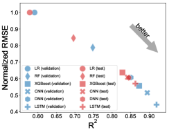
(a) Performance Results

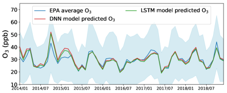
(b) Predicted vs Observed

Figure 2: (a) The performance of six models on the validation and test data. (b) The EPA monthly average O3, DNN model predicted O3 and LSTM model predicted O3 in 2014-2018.

Data	Division rule		LR	RF	XGBoost	CNN	DNN	LSTM
Validation data	sample	slope	0.592	0.710	0.872	0.856	0.872	0.923
		$\textrm{R}^{2}$	0.591	0.748	0.873	0.895	0.872	0.920
		RMSE	11.083	8.732	6.170	5.707	6.724	4.909
	station	slope	0.597	0.702	0.859	0.812	0.439	0.896
		$\textrm{R}^{2}$	0.590	0.733	0.848	0.853	0.994	0.866
		RMSE	11.196	8.942	6.828	6.763	4.148	6.424
	date	slope	0.923	0.698	1.185	0.709	0.894	0.411
		$\textrm{R}^{2}$	0.899	0.984	0.895	0.975	0.890	0.964
		RMSE	4.708	4.646	4.574	4.130	5.740	5.055
Test data	sample	slope	0.572	0.678	0.860	0.829	0.883	0.903
		$\textrm{R}^{2}$	0.578	0.696	0.828	0.842	0.845	0.863
		RMSE	10.855	9.176	6.916	6.603	6.568	6.188
	station	slope	0.576	0.686	0.858	0.826	0.875	0.896
		$\textrm{R}^{2}$	0.577	0.696	0.829	0.840	0.841	0.857
		RMSE	10.861	9.198	6.906	6.641	6.647	6.305
	date	slope	0.571	0.678	0.862	0.820	0.882	0.896
		$\textrm{R}^{2}$	0.578	0.694	0.829	0.842	0.845	0.860
		RMSE	10.856	9.213	6.903	6.606	6.573	6.257

Table 2: The performance of each model on validation and test data. Three division methods to split data for training and validating are used: (1) randomly choosing 10% samples for validation (2) randomly selecting data from 10% stations (3) randomly selecting data from 10% dates in each month. The slope, $\textrm{R}^{2}$, and RMSE for validation data are the average of results from 10-fold CV. Models which have the lowest RSME in 10-fold CV are utilized for test data evaluation. In the test data, the best two performances are in bold and underlined respectively.

3.2 Importance of different factors in predicting O3

The tropospheric O3 formation process is complex and is influenced by many variables. One of our main goals is to understand the influence of individual variables on O3 prediction. Thus, we perform a permutation importance (Altmann et al., 2010) study with the two best performing models DNN and LSTM. The idea is to make one feature randomly unavailable and then compute the drop in model’s performance. Note that this method is also model agnostic. We measure the increase in RMSE ($\rm\Delta$ RMSE) as the drop in model’s performance. The results shown in Fig. 3a suggest that solar radiation is the most significant variable among uncontrollable variables identified by both models. On the other hand, the DNN model emphasizes the significance of $\rm PM_{10}$ while the LSTM model presents the importance of nitrogen monoxide (NO) among variables that are related to human activities and controllable. These results also show that NO2 is another major important anthropogenic variable in O3 prediction. The similarity of two analyses signifies the influence of solar radiation and NO2 in the prediction of O3. Other components having high importance according to the permutation analyses include relative humidity (RH), carbon monoxide (CO), and air temperature. Note that NO, NO2, CO and $\rm PM_{10}$ can be reduced or controlled with better policies such as reduction in fuel combustion and increasing usage of electric vehicles.

We further recognize the nature (positive or negative) of the contribution of each variables in predicting O3 via a recent technique. We employ SHapley Additive exPlanations (SHAP) analysis (Lundberg & Lee, 2017) on DNN and LSTM models. The idea is to use a game theoretic approach called Shapley Values to compute contribution of each individual variable. As displayed in Fig. 3b, the results indicate that while NO and NO2 have strong negative impact, the radiation has extremely positive influence on model-predicted O3.

These results shed some light on the important mechanisms related to O3 formation, as further illustrated in Figure 3c. An interesting observation is that the negative contribution of NO and NO2 might imply that ground-level O3 in Taiwan is mainly constrained by the "NOx-saturated" condition (Sillman, 1999). In other words, reducing the emission of the volatile organic compounds (VOCs), such as benzene, formaldehyde, methanol, and isoprene, might be more efficient than NOx for curtailing the surface O3 concentration in Taiwan. However, the slightly negative contribution of CH4 and non-methane hydrocarbon indicate that reducing these VOCs might not effectively reduce ground-level O3 neither. As a result, the contradiction to the traditional theory could provide a hint for further interesting research directions towards the unrevealed mechanisms of O3 formation. Besides, the high significance of $\rm PM_{10}$ in the permutation analysis of DNN model could not only present the high correlation between $\rm PM_{10}$ and O3 but also be a notion to further explore the possible mechanism for O3 formation on the surface of $\rm PM_{10}$.

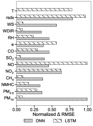
(a) Permutation importance

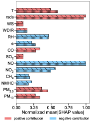
(b) SHAP value of Variables

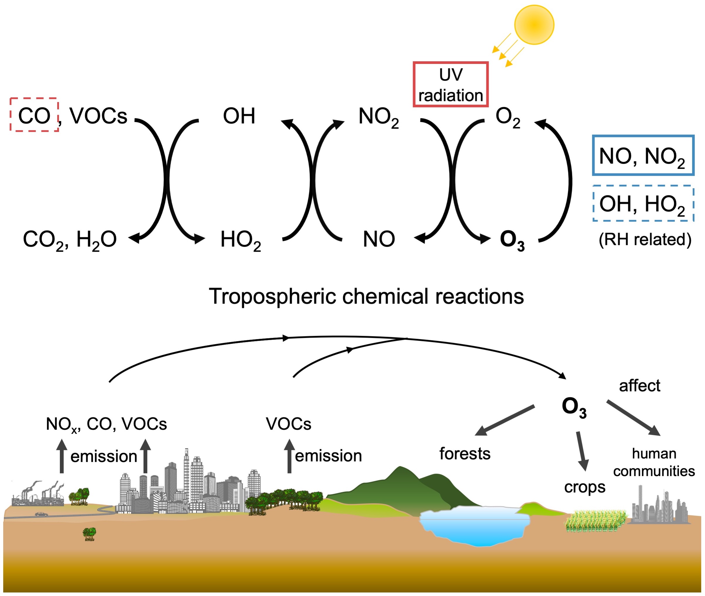
(c) Predicted vs Observed

Figure 3: Importance of variables given by the DNN and LSTM models via two techniques: (a) permutation importance (Altmann et al., 2010) and (b) SHAP (Lundberg & Lee, 2017). The SHAP values are the average values of all input hour. (c) Scheme of the simplified tropospheric O3 formation and decomposition: Anthropogenic trace gases (including NO, NO2 CO, and VOCs) and natural trace gases (some VOCs, such as isoprene and terpenes) can affect the formation and decomposition of O3 directly or indirectly. CO and VOCs can react with OH radical, a significant atmospheric oxidant, to generate HO2 which will further convert NO to NO2. Afterwards, NO2 can react with oxygen (O2) to form O3 in the presence of UV radiation. The produced O3 might get decomposed due to the reaction with NOx and HOx. The generated O3 can severely impact the environment. The most important variables related to predict O3 are solar radiation and NOx family, which contribute positively and negatively to the predicted O3. The minor essential factors are humidity and CO, which contribute negatively and positively to predict O3.

3.3 Evaluation of the impact of climate change and pollution reduction on ground-level O3 concentration

Accurate O3 projection is an important task to help in improving environment related policies that include pollutant emission reduction and damage mitigation. In particular, monitoring and evaluating the impact of O3 on agricultural crops are important since agricultural production losses might cause food crisis and even famine around the world. Here we aim to perform the O3 prediction for different scenarios by applying our proposed DNN and LSTM models. The DNN and LSTM models are able to predict the monthly average data O3 concentration quite accurately (Fig. 2b). Thus, we apply them for analyzing the impact of the pollution reduction and climate change on predicted O3.

Climate change scenarios

”Shared Socioeconomic Pathways” project four different climate change scenarios that are referred as ssp126, ssp245, ssp370, and ssp585 (O’Neill et al., 2016). The ssp126 scenario presumes people to "take the green road" that the world shifts gradually toward a more sustainable path. The ssp245 scenario is a "middle of the road" that the world nearly follows their historical patterns. The ssp370 scenario assumes a “regional rivalry” that weak action is taken on mitigating climate and reducing air pollutant emissions. The ssp585 suspects that the world chooses to accelerate their growth in economic output and energy use. The model simulations based on these four scenarios show that surface temperature over Taiwan is expected to raise 1.0, 1.6, 2.5, and 3.7 ^∘C in by the end of 2100 (2091-2100) compared to 2014-2018 (the period this study focuses). In addition, the water vapor content is supposed to increase 5%, 11%, 17% and 24% in different scenarios. The relative humidity has less change compared to near-surface temperature and water vapor content, as presented in Table 3. We apply our DNN and LSTM models on all of these four scenarios.

	$\Delta$T (∘C)	$\Delta$e (%)	$\Delta$RH (%)
ssp126	1.0	5	-0.2
ssp245	1.6	11	0.4
ssp370	2.5	17	-0.3
ssp585	3.7	24	-0.8

Table 3: The change of three major factors (variables) in CESM2 (Danabasoglu et al., 2020) under ssp126, ssp245, ssp370 and ssp585 scenarios by the end of 21 century (2091-2100) compared to the study period (2014-2018) over Taiwan. $\Delta$T is the average temperature change in degrees Celsius. $\Delta$e and $\Delta$RH are the water vapor change and relative humidity change in percentage, respectively.

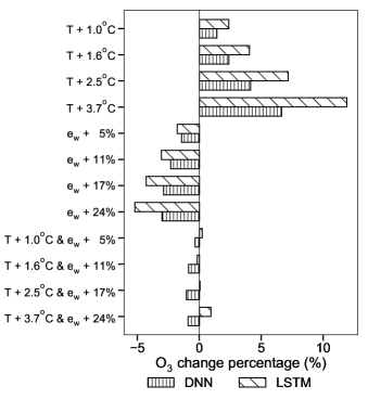
(a) Climate change scenarios

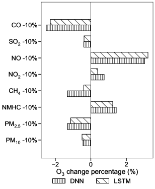
(b) Pollution controlling scenarios

Figure 4: The predicted O3 change under (a) climate change scenarios and (b) pollution controlling scenarios. (a) Significant increase in temperature and water vapor content in the different CESM2 simulation based on four SSP assumptions is considered and applied our test dataset in DNN and LSTM models. (b) Besides, we consider the reduction of 10% of each anthropogenic variables in the test dataset in DNN and LSTM models.

3.3.1 Simulation of climate change and pollution reduction

Simulation of climate change

As advised by the model simulation results, we apply the mentioned temperature and water vapor content increase to our test data (the observation during 2018) separately and together with the remaining variables unchanged and predict their effect on O3 concentration. Figure 4a presents the results. The DNN and LSTM models both indicate that increasing temperature could raise O3 concentration while increasing water vapor content could lower O3 concentration. While the positive contribution of temperature increase could significantly raise O3, the negative contribution of water content vapor increase is able to offset the effect of temperature increase. Consequently, the change in O3 becomes negligible when considering the perturbation of these two variables together (as shown in Figure 4a).

Simulation of pollution reduction

The above results indicate that the reduction of anthropogenic pollutants might be more crucial for controlling O3 in the future. Reducing pollution is always an important policy move in most countries for improving public health in general. However, controlling different pollutants can have a distinct impact on O3 concentration. Thus, we study the effect of reducing 10% of each anthropogenic pollutant value on the predicted O3 in test dataset applying DNN and LSTM models. Figure 4b shows the results which demonstrate that reducing 10 percent CO would have the most apparent effect on decreasing ground-level O3 among all anthropogenic variables found by both models. Again, though controlling the emission of CO could contribute to lower O3, reducing the amount of NO and NO2 might lead to an increment of O3. Therefore, simulations with different pollution control strategies by global climate models are still necessary to have a more comprehensive evaluation.

Discussion

As presented in Fig. 4b, reducing CO, CH4, and $\rm PM_{2.5}$ could be important for decreasing O3 concentration. Anthropogenic CO comes from the incomplete combustion of carbon-based fuel, and major CO sources include transportation and industrial activity. The generation of CH4, another major greenhouse gas, is also highly co-related to human activity, such as agriculture, fossil fuel extraction, wildfire, and biomass burning. $\rm PM_{2.5}$ are aerosols with complicated composition and can be directly emitted or formed via sophisticated chemical reactions of gases including NOx, SO2, and VOCs. To reduce CO, CH4, and $\rm PM_{2.5}$, it will be important to decrease the use of fuel vehicles and carbon-containing fuel and raise the percentage of renewable energy. However, reducing anthropogenic gases means that the concentrations of NO and NO2 would also decrease. The negative contribution of NO and NO2 must be carefully studied to evaluate the total effect of reducing anthropogenic gases to the future O3 concentration. These results clearly show the various kinds of actions where the government should have a stricter policy to make a better environment for the future.

4 Conclusions

In this study, we have predicted tropospheric O3 which is one of the greenhouse gas and an influential ground-level air pollutant that can severely damage the environment. We have compared six methods to estimate the tropospheric O3 concentration and understand the importance of some meteorological variables, trace gases and pollutants in forming the ground-level O3. The importance of solar radiation is emphasized in the best two models, DNN and LSTM models, which conform to the theoretical study. However, all NOx and volatile organic compounds (VOCs) are presented to contribute negatively to O3 prediction, which contradicts the O3 and NOx-VOCs relationship. This would promote a direction for future research about undiscovered O3 formation mechanisms. Moreover, the study regarding the importance of the variables or factors will lead to better policy makings to control the production of such materials or pollutants. We have further investigated the O3 concentration under different scenarios and shown that controlling anthropogenic gases, especially CO, could be critical for reducing O3 in the future considering the facts that the surface temperature and water vapor content may increase. Our findings clearly show the various kind of actions that the government should have stricter policies on, to make a better environment for the future.

References

- Ainsworth (2017) Elizabeth A. Ainsworth. Understanding and improving global crop response to ozone pollution. The Plant Journal, 90(5):886–897, 2017.
- Altmann et al. (2010) André Altmann, Laura Toloşi, Oliver Sander, and Thomas Lengauer. Permutation importance: a corrected feature importance measure. Bioinformatics, 26(10):1340–1347, 2010.
- Bessho et al. (2016) Kotaro Bessho, Kenji Date, Masahiro Hayashi, Akio Ikeda, Takahito Imai, Hidekazu Inoue, Yukihiro Kumagai, Takuya Miyakawa, Hidehiko Murata, Tomoo Ohno, et al. An introduction to himawari-8/9—japan’s new generation geostationary meteorological satellites. Journal of the Meteorological Society of Japan. Ser. II, 94(2):151–183, 2016.
- Danabasoglu et al. (2020) G. Danabasoglu, J.-F. Lamarque, J. Bacmeister, D. A. Bailey, A. K. DuVivier, J. Edwards, L. K. Emmons, J. Fasullo, R. Garcia, A. Gettelman, et al. The Community Earth System Model Version 2 (CESM2). Journal of Advances in Modeling Earth Systems, 12(2):e2019MS001916, 2020.
- Danabasoglu (2019a) Gokhan Danabasoglu. Ncar cesm2 model output prepared for cmip6 cmip historical, 2019a.
- Danabasoglu (2019b) Gokhan Danabasoglu. Ncar cesm2 model output prepared for cmip6 scenariomip ssp126, 2019b.
- Danabasoglu (2019c) Gokhan Danabasoglu. Ncar cesm2 model output prepared for cmip6 scenariomip ssp245, 2019c.
- Danabasoglu (2019d) Gokhan Danabasoglu. Ncar cesm2 model output prepared for cmip6 scenariomip ssp370, 2019d.
- Danabasoglu (2019e) Gokhan Danabasoglu. Ncar cesm2 model output prepared for cmip6 scenariomip ssp585, 2019e.
- Eslami et al. (2019) Ebrahim Eslami, Yunsoo Choi, Yannic Lops, and Alqamah Sayeed. A real-time hourly ozone prediction system using deep convolutional neural network. Neural Computing and Applications, pp. 1–15, 2019.
- Lundberg & Lee (2017) Scott M Lundberg and Su-In Lee. A Unified Approach to Interpreting Model Predictions. In Advances in Neural Information Processing Systems 30, pp. 4765–4774. 2017.
- Nowack et al. (2018) Peer Nowack, Peter Braesicke, Joanna Haigh, Nathan Luke Abraham, John Pyle, and Apostolos Voulgarakis. Using machine learning to build temperature-based ozone parameterizations for climate sensitivity simulations. Environmental Research Letters, 13(10):104016, 2018.
- O’Neill et al. (2016) B. C. O’Neill, C. Tebaldi, D. P. van Vuuren, V. Eyring, P. Friedlingstein, G. Hurtt, R. Knutti, E. Kriegler, J.-F. Lamarque, J. Lowe, G. A. Meehl, R. Moss, K. Riahi, and B. M. Sanderson. The scenario model intercomparison project (scenariomip) for cmip6. Geoscientific Model Development, 9(9):3461–3482, 2016.
- Seinfeld & Pandis (2016) John H. Seinfeld and Spyros N. Pandis. Atmospheric Chemistry and Physics: from air pollution to climate change. John Wiley & Sons, 2016.
- Sillman (1999) Sanford Sillman. The relation between ozone, NOx and hydrocarbons in urban and polluted rural environments. Atmospheric Environment, 33(12):1821 – 1845, 1999.
- Stevenson et al. (2013) D. S. Stevenson, P. J. Young, V. Naik, J.-F. Lamarque, D. T. Shindell, A. Voulgarakis, R. B. Skeie, S. B. Dalsoren, G. Myhre, T. K. Berntsen, G. A. Folberth, S. T. Rumbold, W. J. Collins, I. A. MacKenzie, R. M. Doherty, G. Zeng, T. P. C. van Noije, A. Strunk, D. Bergmann, P. Cameron-Smith, D. A. Plummer, S. A. Strode, L. Horowitz, Y. H. Lee, S. Szopa, K. Sudo, T. Nagashima, B. Josse, I. Cionni, M. Righi, V. Eyring, A. Conley, K. W. Bowman, O. Wild, and A. Archibald. Tropospheric ozone changes, radiative forcing and attribution to emissions in the atmospheric chemistry and climate model intercomparison project (accmip). Atmospheric Chemistry and Physics, 13(6):3063–3085, 2013.
- Watson et al. (2019) Gregory L. Watson, Donatello Telesca, Colleen E. Reid, Gabriele G. Pfister, and Michael Jerrett. Machine learning models accurately predict ozone exposure during wildfire events. Environmental Pollution, 254:112792, 2019.
- Young et al. (2018) Paul John Young, Vaishali Naik, Arlene M Fiore, Audrey Gaudel, Jean Guo, MY Lin, Jessica Neu, David Parrish, HE Reider, JL Schnell, et al. Tropospheric Ozone Assessment Report: Assessment of global-scale model performance for global and regional ozone distributions, variability, and trends. Elementa: Science of the Anthropocene, 6(1), 2018.