Testing the intrinsic scatter of the asteroseismic scaling relations with Kepler red giants

Abstract

Asteroseismic scaling relations are often used to derive stellar masses and radii, particulaly for stellar, exoplanet, and Galactic studies. It is therefore important that their precisions are known. Here we measure the intrinsic scatter of the underlying seismic scaling relations for $\Delta\nu$ and $\nu_{\rm max}$, using two sharp features that are formed in the H–R diagram (or related diagrams) by the red giant populations. These features are the edge near the zero-age core-helium-burning phase, and the strong clustering of stars at the so-called red giant branch bump. The broadening of those features is determined by factors including the intrinsic scatter of the scaling relations themselves, and therefore it is capable of imposing constraints on them. We modelled Kepler stars with a Galaxia synthetic population, upon which we applied the intrinsic scatter of the scaling relations to match the degree of sharpness seen in the observation. We found that the random errors from measuring $\Delta\nu$ and $\nu_{\rm max}$ provide the dominating scatter that blurs the features. As a consequence, we conclude that the scaling relations have intrinsic scatter of $\sim 0.5\%$ ($\Delta\nu$), $\sim 1.1\%$ ($\nu_{\rm max}$), $\sim 1.7\%$ ($M$) and $\sim 0.4\%$ ($R$), for the SYD pipeline measured $\Delta\nu$ and $\nu_{\rm max}$. This confirms that the scaling relations are very powerful tools. In addition, we show that standard evolution models fail to predict some of the structures in the observed population of both the HeB and RGB stars. Further stellar model improvements are needed to reproduce the exact distributions.

1 Introduction

The asteroseismic scaling relations for red giants have so far proved to be an extremely useful tool to obtain stellar masses and radii. A critical issue associated with the scaling relations is that their limits are poorly understood (Hekker, 2020). The intrinsic scatter of the scaling relations, originating from potential hidden dependencies not accounted for in the current relations, can cause a seemingly random fluctuation. Testing the intrinsic scatter of these relations is the aim of this paper.

The scaling relations rely on two characteristic frequencies in the power spectra of solar-like oscillations. The first one is $\Delta\nu$, the large separation of p modes, approximately proportional to the square root of mean density (Ulrich, 1986):

$$\frac{\Delta\nu}{\Delta\nu_{\astrosun}}\approx\left(\frac{M}{M_{\astrosun}}\right)^{1/2}\left(\frac{R}{R_{\astrosun}}\right)^{-3/2}.$$ (1)

The second is $\nu_{\rm max}$, which is the frequency where the power of the oscillations is strongest. It relates to the surface properties $g/\sqrt{T_{\rm eff}}$ (Brown et al., 1991; Kjeldsen & Bedding, 1995):

$$\frac{\nu_{\rm max}}{\nu_{\rm max,\astrosun}}\approx\left(\frac{M}{M_{\astrosun}}\right)\left(\frac{R}{R_{\astrosun}}\right)^{-2}\left(\frac{T_{\rm eff}}{T_{\rm eff,\astrosun}}\right)^{-1/2}.$$ (2)

Using these, the mass and radius can be determined if the effective temperature is known (Stello et al., 2008; Kallinger et al., 2010a):

$$\frac{M}{M_{\astrosun}}\approx\left(\frac{\nu_{\rm max}}{\nu_{\rm max,\astrosun}}\right)^{3}\left(\frac{\Delta\nu}{\Delta\nu_{\astrosun}}\right)^{-4}\left(\frac{T_{\rm eff}}{T_{\rm eff,\astrosun}}\right)^{3/2},$$ (3)

$$\frac{R}{R_{\astrosun}}\approx\left(\frac{\nu_{\rm max}}{\nu_{\rm max,\astrosun}}\right)\left(\frac{\Delta\nu}{\Delta\nu_{\astrosun}}\right)^{-2}\left(\frac{T_{\rm eff}}{T_{\rm eff,\astrosun}}\right)^{1/2}.$$ (4)

From a theoretical point of view, a more accurate value for $\Delta\nu$ can be calculated from oscillation frequencies given a stellar model; thus it is possible to map the departure of Eq. 1, as a function of [M/H], $M$, $T_{\text{eff}}$ and evolutionary state (White et al., 2011; Sharma et al., 2016; Guggenberger et al., 2016; Rodrigues et al., 2017; Serenelli et al., 2017; Pinsonneault et al., 2018). Improvements are seen when adopting this revised theoretical $\Delta\nu$ over the standard density scaling (e.g. Brogaard et al., 2018). However, there are some degrees of uncertainty. Christensen-Dalsgaard et al. (2020) found a 0.2% spread in the theoretical departure stemming from implementing the calculation with different codes, and the degree of model-dependency on physical processes has not been explored extensively.

The $\nu_{\rm max}$ scaling relation is much harder to assess theoretically because calculating $\nu_{\rm max}$ would require a detailed treatment of non-adiabatic processes, via either 1D or 3D stellar models (e.g. Balmforth, 1992; Houdek et al., 1999; Belkacem et al., 2019; Zhou et al., 2019). Some works concluded a possible departure could correlate with, for example, the Mach number (Belkacem et al., 2011), magnetic activity (Jiménez et al., 2011) and mean molecular weight (Jiménez et al., 2015; Yıldız et al., 2016; Viani et al., 2017). In general, it is still impossible to accurately predict $\nu_{\rm max}$ from theory.

Another way to test the scaling relations is by comparing with fundamental data from independent observations. This requires masses and radii obtained by other means, such as astrometric surveys, where radii are deduced using the Stefan-Boltzmann law, eclipsing binaries, where masses and radii are derived from dynamic modelling. So far, the radii tests based on parallaxes suggest agreement within 4% for stars smaller than 30 $R_{\astrosun}$ (Silva Aguirre et al., 2012; Huber et al., 2017; Sahlholdt & Silva Aguirre, 2018; Hall et al., 2019; Khan et al., 2019; Zinn et al., 2019). With 16 eclipsing binaries, Gaulme et al. (2016) found the asteroseismic masses and radii are systematically overestimated, by factors of 15% and 5%, respectively. This result is in disagreement with Gaia radii, possibly because the binary temperature is affected by blending (Huber et al., 2017; Zinn et al., 2019). Subsequent analyses indicate that the main source of departure could come from the $\Delta\nu$ scaling relation (Brogaard et al., 2018; Sharma et al., 2019).

As we noted earlier, the random departures of the scaling relations can be associated with unaccounted factors, for example, metallicity, rotation and magnetism, some of which are known to have a wide-ranging distribution among red giants (e.g. Mosser et al., 2012; Stello et al., 2016; Ceillier et al., 2017). They could be responsible for some intrinsic scatter in these rather simple relations.

We propose a new approach to investigate the intrinsic scatter, based on two sharp features in the H–R diagram observed among the red giant population. The first feature is the accumulation of stars at the bump of red-giant-branch (RGB). The second feature is the sharp edge formed by the zero-age sequence of core-helium-burning (HeB) stars. These features were known before seismic observations became available.

The RGB bump is an evolutionary stage where a star ascending the RGB temporarily drops in luminosity before again ascending towards the tip of the RGB, causing a hump in the luminosity distribution. This feature is prominent in colour-magnitude diagrams of stellar clusters (Iben, 1968; King et al., 1985). The luminosity drop takes place after the first dredge-up and is caused by a change in the composition profile near the hydrogen-burning shell, leading to a decrease in mean molecular weight outside the composition discontinuity point (Refsdal & Weigert, 1970; Christensen-Dalsgaard, 2015). Kepler data show that this bump is also present in the distributions of $\Delta\nu$ and $\nu_{\rm max}$ (Kallinger et al., 2010b; Khan et al., 2018).

After reaching the tip of RGB, stars strongly decrease in luminosity and commence core helium burning, forming the red clump, also commonly recognised as the horizontal branch in metal-poor clusters (Cannon, 1970; Girardi et al., 2010). The low-luminosity edge defines the beginning of the red clump and secondary clump phase, which we we will refer to as the zero-age HeB (ZAHeB) phase. This feature is also imprinted on seismic observables (Kallinger et al., 2010b; Huber et al., 2010; Mosser et al., 2010; Yu et al., 2018).

The fact that the seismic parameters ($\Delta\nu$ and $\nu_{\rm max}$) preserve these sharp features indicates that the seismic parameters must be tightly related to the fundamental stellar parameters. Put another way, if there were a large intrinsic scatter in the scaling relations, the features in the seismic diagrams would not be as sharp. Using this principle, we can quantify the limits on the intrinsic scatter in the scaling relations. That is the aim of this paper.

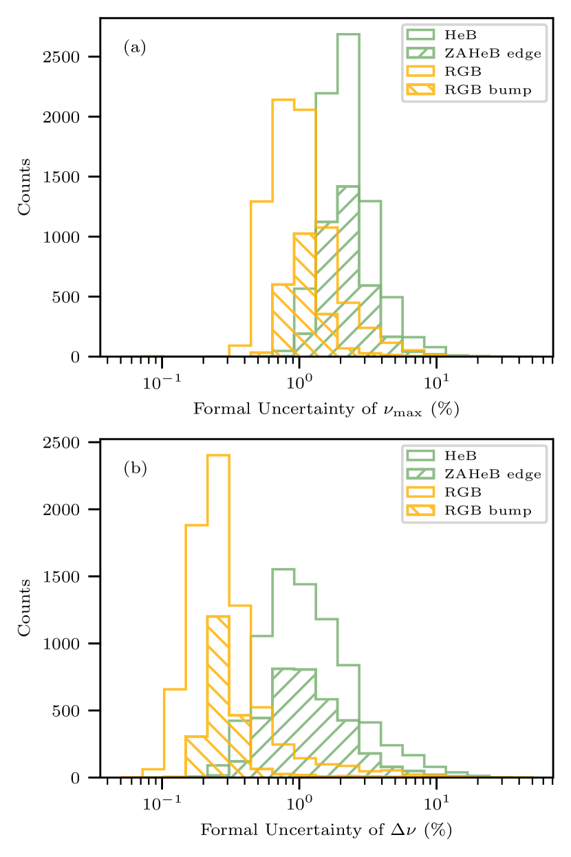
Figure 1: Distributions of the SYD18 formal uncertainties of the $\nu_{\rm max}$ and $\Delta\nu$ measurements.

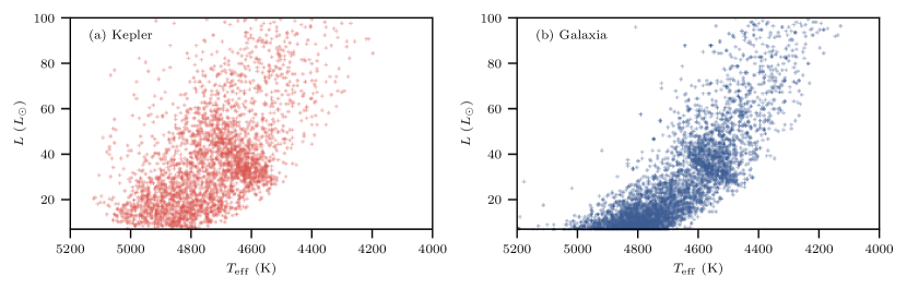
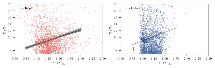
Figure 2: $L$ vs. $T_{\text{eff}}$ (panels a–b), $\nu_{\rm max}$ vs. $T_{\text{eff}}$ (panels c–d), $\Delta\nu$ vs. $T_{\text{eff}}$ (panels e–f) and $R$ vs. $M$ (bottom g–h) for RGB stars in the APK18 sample (red) and the G19 sample (blue). The RGB bumps were defined using the black straight fiducial lines. The grey-shaded areas denote the uncertainty of identifying the bump (see 5.1.2).

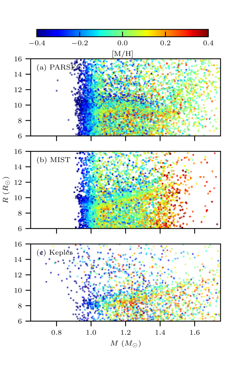
Figure 3: Radius vs. mass for RGB stars near the RGB bump, colour-coded by metallicity. The PARSEC and MIST isochrones predict different outcomes on the shape of the RGB bump.

2 Sample selection

To create our sample we used the red giants observed by Kepler, with $\Delta\nu$ and $\nu_{\rm max}$ measured by the SYD pipeline (Huber et al., 2009; Yu et al., 2018), and classifications of evolutionary stage (RGB/HeB) from Hon et al. (2017). We denote this sample as SYD18, including 7543 HeB stars and 7534 RGB stars. A subset of 2531 HeB and 3308 RGB stars with $T_{\text{eff}}$ and [M/H] from the APOKASC-2 catalog (Pinsonneault et al., 2018) was also used, denoted as APK18. In Fig. 1, we show the distributions of the formal uncertainties of $\nu_{\rm max}$ and $\Delta\nu$ measured by SYD18. The SYD18 sample reports a typical formal uncertainty of $2.1\%$ on $\nu_{\rm max}$ and $1.0\%$ on $\Delta\nu$ in HeB stars, and $0.95\%$ on $\nu_{\rm max}$ and $0.3\%$ on $\Delta\nu$ in RGB stars.

To model the observed population, we used a synthetic sample produced by Sharma et al. (2019) with a Galactic model, Galaxia (Sharma et al., 2011). Compared to a previous synthetic sample in Sharma et al. (2016), the synthetic sample we used in this work adds a metal-rich thick disc, which improves the overall match with the Kepler observation (Sharma et al., 2019). Here we denote this sample as G19. The G19 simulated sample is about ten times larger than the SYD18 sample. Each star in the simulated sample is associated with an initial mass, an age, and a metallicity, sampled from a Galactic distribution function and passed through a selection function tied to the Kepler mission. Other fundamental stellar parameters (e.g. $M$, $R$ and $T_{\text{eff}}$) were estimated via two different sets of theoretical isochrones: PARSEC (Marigo et al., 2017) and MIST (Choi et al., 2016). Both isochrones include some mass loss along the RGB, using the Reimers (1975) prescription with an efficiency of $\eta_{R}=0.2$ (PARSEC) and $\eta_{R}=0.1$ (MIST), consistent with the asteroseismology of open clusters (Miglio et al., 2012). The seismic parameters, $\Delta\nu$ and $\nu_{\rm max}$, were calculated through the scaling relations (Eqs. 1 and 2) without any corrections. By examining the sharpness of the two features discussed above, and comparing the Galaxia simulation with the observations, we are able to draw conclusions about the intrinsic scatter of the scaling relations.

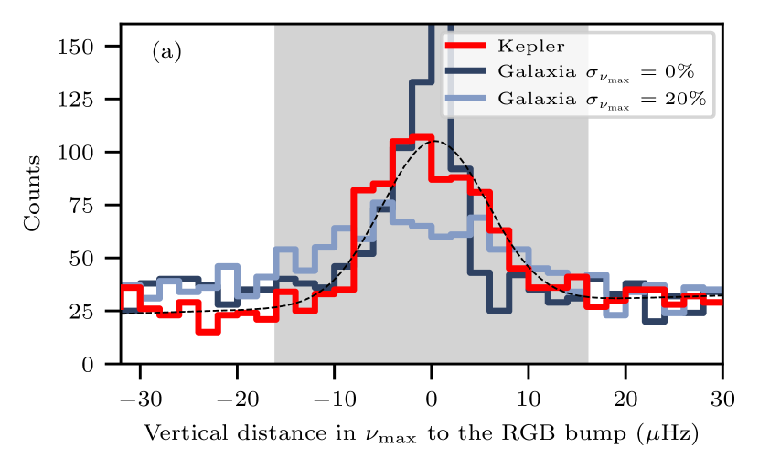
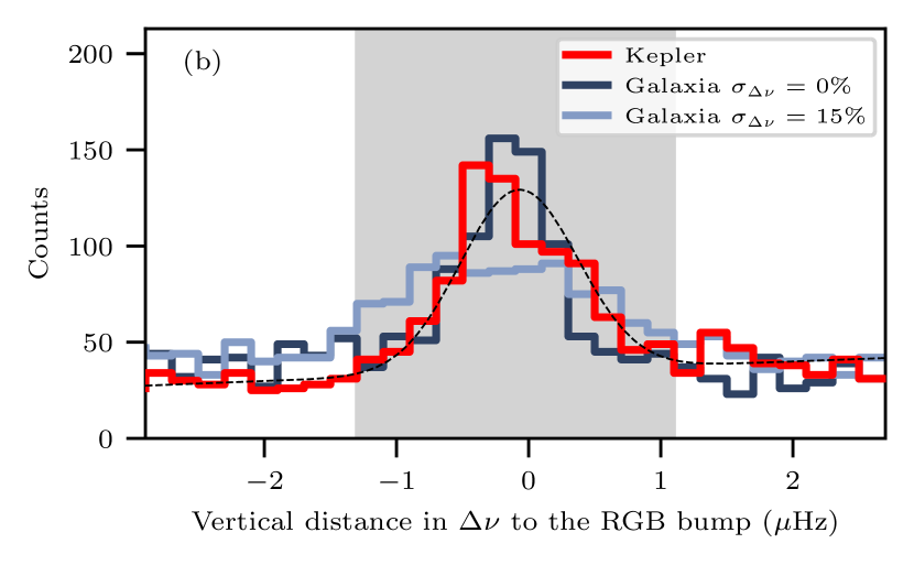
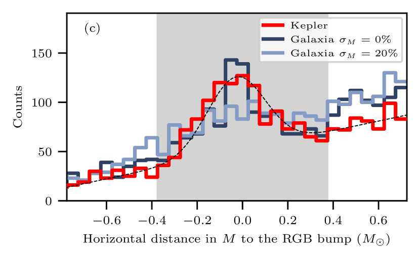
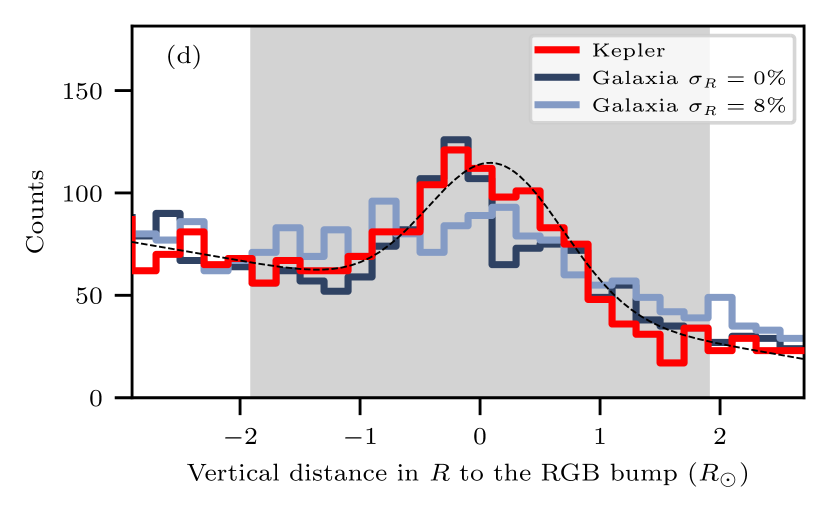
Figure 4: Distributions of distances to the bump features. The top two panels are measured in the $T_{\text{eff}}$–$\nu_{\rm max}$ and $T_{\text{eff}}$–$\Delta\nu$ diagrams, and the bottom two panels are measured in the $M$–$R$ diagram. The Kepler (APK18) distributions are shown in red, fitted with a Gaussian model, denoted by the black dashed lines. The synthetic G19 samples are shown in blue. The grey-shaded areas denote the range used to compare the data.

3 The RGB bump

In this section, we look at the RGB bump. In a traditional H–R diagram, the bump is tilted so that the luminosity $L$ of the bump is a function of $T_{\text{eff}}$ and its shape can be parameterized by stellar mass $M$, using $L=L(M)$ and $T_{\rm eff}=T_{\rm eff}(M)$. By introducing the $\nu_{\rm max}$ scaling relation, we can obtain $\nu_{\rm max}\propto ML^{-1}T_{\rm eff}^{7/2}$. Therefore, a narrow bump in the $L$–$T_{\text{eff}}$ plane will also show a bump due to this $M$ dependence in the $\nu_{\rm max}$–$T_{\text{eff}}$ plane. If the $\nu_{\rm max}$ scaling relation has some intrinsic scatter due to other dependencies, such as metallicity, then the observed bump in the $\nu_{\rm max}$–$T_{\text{eff}}$ plane could be wider.

For $\Delta\nu$, the argument is similar. Fig. 2 shows the RGB bump for both Kepler and Galaxia samples. Here we wish to model the width of the RGB bump. We will start by investigating the features in the $\Delta\nu$–$T_{\text{eff}}$ and $\nu_{\rm max}$–$T_{\text{eff}}$ diagrams, and then in the $M$–$R$ diagram.

We further note that the width of RGB bump strongly depends on how the physical processes are modelled in the isochrones. This is illustrated in Fig. 3, where the shapes of the RGB bump predicted by the two sets of isochrones are inconsistent. The PARSEC models predict that the stellar radii at the RGB bump should decrease with masses for masses larger than $\sim$1.2 $M_{\astrosun}$. However, the opposite is observed in the Kepler samples, and this behaviour is correctly described by the MIST models. It implies that the RGB bump may not serve as a useful diagnostic for the scaling relations. We will examine this caveat more extensively in section 5.1.1. Nevertheless, here we still use the RGB bump to introduce our method and we analyse the G19 samples with the two isochrones separately.

3.1 Modelling method

We used a forward-modelling approach by constructing synthetic samples based on the G19 sample, and setting the intrinsic scatter of the scaling relations, $\sigma$, as a free parameter. The width of the bump was evaluated by measuring the distances of model samples to the centre of the bump, and fitting their distributions to the APK18 sample.

The first step was to define the locations of the RGB bump in the APK18 and G19 samples with straight lines in the $\nu_{\rm max}$–$T_{\text{eff}}$ and $\Delta\nu$–$T_{\text{eff}}$ diagrams, shown in Fig. 2.

We generated a synthetic population by adding random scatter to the G19 sample. Each physical quantity $x$ (one of $\Delta\nu$, $\nu_{\rm max}$, $M$ or $R$) for the $i$-th star in the sample was

$$x_{i}=x_{{\textit{Galaxia}},i}(1+\sigma_{{\rm total},i}).$$ (5)

The quantity $x_{{\textit{Galaxia}},i}$ is the physical value without any perturbation. For $M$ and $R$, they were directly estimated from isochrones. Note that $M$ is the actual mass rather than the initial mass. Values for $\Delta\nu$ and $\nu_{\rm max}$ were determined via scaling relations (Eqs. 1 and 2) and further corrected using oscillation frequencies ($\Delta\nu$ in particular, see section 3.2). We modelled the total scatter needed to reproduce the width of the RGB bump, $\sigma_{{\rm total},i}$, which was drawn from a normal distribution with a standard deviation $\sigma_{\rm total}$.

To account for the scatter induced by the formal uncertainties of the $\Delta\nu$ and $\nu_{\rm max}$ measurements, we modelled each quantity $x$ with

$$x_{i}=x_{{\textit{Galaxia}},i}(1+\sigma_{x,i}+\sigma_{{\rm SR},i}),$$ (6)

where $\sigma_{x,i}$ represents the fractional uncertainty of $x_{{\textit{Galaxia}},i}$, and was drawn randomly from the APK18 formal uncertainty distribution of RGB bump stars. The intrinsic scatter in the scaling relation was modelled via $\sigma_{{\rm SR},i}$, drawn from a normal distribution with a standard deviation $\sigma_{{\rm SR}}$.

We then calculated the distributions of distances to bump lines. The bump lines, shown in Fig. 2, were picked so that the distances to the line have the smallest standard deviation. For $\Delta\nu$ and $\nu_{\rm max}$, we calculated the vertical distances in the $\Delta\nu$–$T_{\text{eff}}$ and $\nu_{\rm max}$–$T_{\text{eff}}$ diagrams, respectively. For $M$ and $R$, we used the horizontal and vertical distances in the $M$–$R$ diagram. This procedure allowed us to investigate the scatter in each relation separately, because perturbing the horizontal value will not change the vertical value, and vice versa. In Fig. 4, we plot the distributions of those distances with two representative choices for $\sigma_{\rm{total}}$. A larger value for $\sigma_{\rm{total}}$ flattens the hump, demonstrating the width of the bump itself provides a measure of the intrinsic scatter in the scaling relations.

Next, we introduce our fitting strategy to enable the comparison, which is to match the counts in each bin of the histograms. We first identified a central region in the histograms of the APK18 sample by fitting a Gaussian profile plus a sloping straight line, illustrated by the dashed curves in Fig. 4. The central region was defined to be a range centred around the Gaussian, with a width of 6 times the Gaussian standard deviation. In Fig. 4, they are shown in grey-shaded areas. In our fit described below, we matched the distributions in the central regions only.

Because the G19 sample is larger than the APK18 sample, we re-scaled the number of model samples by normalising according to the APK18 sample in the central region. We also added a constant $c$ as a free parameter to the distance of the model samples, in order to compensate for a possible offset of maxima, which could originate from a bias in identifying the bump.

We optimised the likelihood function, assuming the distribution of counts in each bin is set by Poisson statistics:

$$\ln L=\sum_{m_{j}\neq 0}\left[d_{j}\ln m_{j}-m_{j}-\ln(d_{j}!)\right],$$ (7)

where $d_{j}$ and $m_{j}$ are counts in the $j$-th bins of the Kepler and model distributions. This fitting method is commonly used in population studies to constrain the star formation history, initial mass function and binary properties (e.g. Dolphin, 2002; Geha et al., 2013; El-Badry et al., 2019). The posterior distributions of parameters $c$ and $\sigma$ were sampled with uninformative flat priors, using a Markov Chain Monte Carlo (MCMC) method. We used 200 white walkers, burned-in for 500 steps to reach convergence and then iterated for another 1000 steps. The medians and 68% credible uncertainties of the parameters were estimated from the posteriors directly.

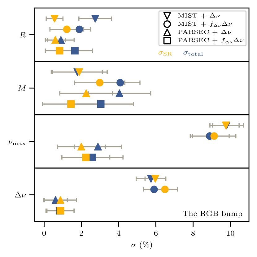
Figure 5: Intrinsic scatter of the scaling relations $\sigma_{\rm SR}$ (yellow) and total scatter $\sigma_{\rm total}$ (blue), derived using the width of the RGB bump.

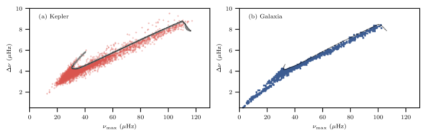
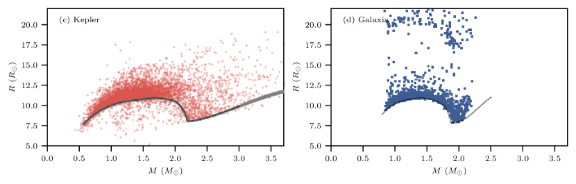
Figure 6: $\nu_{\rm max}$–$\Delta\nu$ diagram (panels a–b) and $M$–$R$ diagram (panels c–d) for HeB stars in the SYD18 sample (red) and the G19 sample (blue). The zero-age HeB edges were defined using splines, shown as the black lines. The grey-shaded areas denote the uncertainty of identifying the edges (see section 5.1.2). The stars around $20$ $R_{\astrosun}$ in the G19 sample are at the asymptotic-giant-branch phase.

3.2 Results

Our first step is to derive the total scatter responsible for the width of the RGB bump, $\sigma_{\rm total}$, in Eq. 5. We obtained $0.61\%$ ($\Delta\nu$), $2.89\%$ ($\nu_{\rm max}$), $4.05\%$ ($M$) and $0.90\%$ ($R$) with PARSEC, and $5.74\%\pm 0.80\%$ ($\Delta\nu$), $9.80\%\pm 0.90\%$ ($\nu_{\rm max}$), $1.79\%\pm 1.34\%$ ($M$) and $2.75\%\pm 0.88\%$ ($R$) with MIST.

Next we took the formal uncertainties of the $\Delta\nu$ and $\nu_{\rm max}$ measurements into account and obtained the limits on the intrinsic scatter of the scaling relations, $\sigma_{\rm SR}$, in Eq. 6. With PARSEC, we obtained $0.88\%$ ($\Delta\nu$), $2.00\%$ ($\nu_{\rm max}$), $2.26\%$ ($M$) and $0.60\%$ ($R$). With MIST, we obtained $5.97\%$ ($\Delta\nu$), $9.76\%$ ($\nu_{\rm max}$), $1.89\%$ ($M$) and $0.56\%$ ($R$). These numbers are plotted in Fig. 5. There is a huge difference between MIST and PARSEC. We will discuss it in section 5.1.1.

4 The ZAHeB edge

Similar to the RGB bump, the zero-age sequence of HeB stars (ZAHeB) also forms a well-defined feature in the H–R diagram (Girardi et al., 2010; Girardi, 2016). We note that the transition from the red clump (low-mass stars that ignite helium in a fully degenerate core) to the secondary red clump (higher-mass stars that ignite helium in a partly or non-degenerate core) is smooth and continuous (Girardi, 2016). Given the scaling relations, there should exist a close correlation between $\Delta\nu$ and $\nu_{\rm max}$ for the ZAHeB.

In Fig. 6, we show the HeB stars in the $\Delta\nu$–$\nu_{\rm max}$ and $M$–$R$ diagrams. The ZAHeB appears as a very sharp feature: all HeB stars are located at only one side of the ZAHeB, forming a remarkably sharp edge. Now we use the sharpness of this edge to quantify the intrinsic scatter of the scaling relations.

4.1 Modelling method

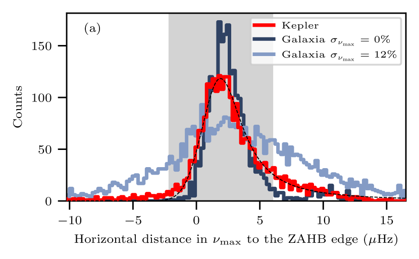
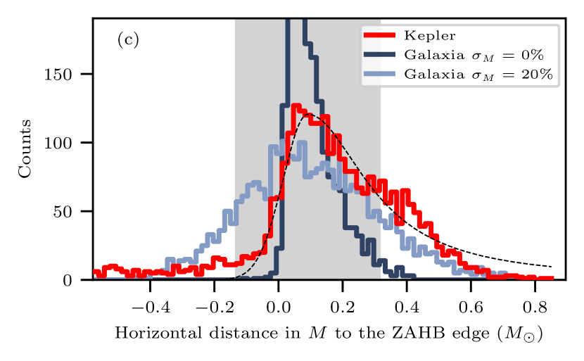
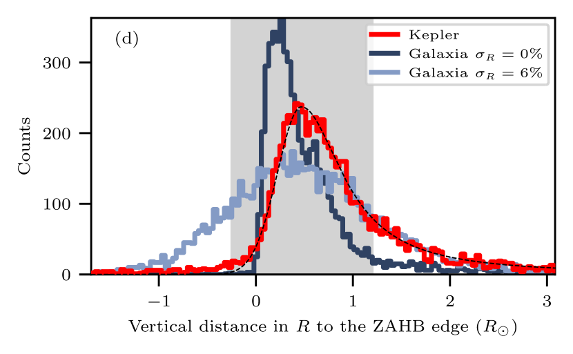
Figure 7: Distributions of distances to the ZAHeB edges. The top two panels are measured in the $\nu_{\rm max}$–$\Delta\nu$ diagram, and the bottom two panels are measured in the $M$–$R$ diagram. The Kepler (SYD18) distributions are shown in red, fitted with a half-Gaussian-half-Lorentzian model, denoted by the black dashed lines. The synthetic G19 samples are shown in blue. The grey-shaded areas denote the range used to compare the data.

To measure the sharpness of the ZAHeB edge, we used a modelling method similar to that for the RGB bump in section 3.1, but with three important differences.

The first difference is related to defining the location of the feature. For RGB stars, we used straight lines to denote the location of the bump. For HeB stars, we used splines in the $\Delta\nu$–$\nu_{\rm max}$ and $M$–$R$ diagrams to define the ZAHeB edges. This is illustrated in Fig. 6, where the edges are shown as black lines.

The second difference is how we calculated the horizontal and vertical distances to the ZAHeB edge. In the $\Delta\nu$–$\nu_{\rm max}$ diagram, the stars below the lowest point of the edge do not have a meaningful horizontal distance. We therefore excluded them for the horizontal distance calculation. The same strategy was also applied to all stars that lie on the left of the leftmost point of the defined ZAHeB edge when calculating vertical distances. Similarly, in the $M$–$R$ diagram, the stars above the highest point of the ZAHeB edge were not considered in calculating horizontal distances. In Fig. 7, we plot the distributions of those distances with two $\sigma_{\rm total}$. As for the RGB bump, we see that a larger scatter $\sigma_{\rm total}$ smooths the hump.

The third difference is that, in order to choose regions near each edge to compare, we fitted a profile to the distributions for the SYD18 sample. The profiles, shown as the dashed lines in Fig. 7, consisted of a half Gaussian (left) and a half Lorentzian (right). The histogram region that we fitted was a range centred at the Gaussian’s centre, with a width of 6 times the Gaussian’s standard deviation. These regions are shown as grey-shaded areas.

4.2 Results

Figure 8: Intrinsic scatter of the scaling relations $\sigma_{\rm SR}$ (yellow) and total scatter $\sigma_{\rm total}$ (blue), derived using the sharpness of the ZAHeB edge.

We measured the total scatter $\sigma_{\rm total}$ that contributes to the broadening of the edges in the $\nu_{\rm max}$–$\Delta\nu$ and $M$–$R$ diagrams: $1.25\%\pm 0.05\%$ ($\Delta\nu$), $2.23\%\pm 0.12\%$ ($\nu_{\rm max}$), $9.10\%\pm 0.50\%$ ($M$) and $2.01\%\pm 0.05\%$ ($R$) using the PARSEC models, and $1.56\%\pm 0.04\%$ ($\Delta\nu$), $2.99\%\pm 0.19\%$ ($\nu_{\rm max}$), $7.00\%\pm 0.54\%$ ($M$) and $2.29\%\pm 0.07\%$ ($R$) using the MIST models. These numbers are in general agreement with the formal uncertainties of $\Delta\nu$ and $\nu_{\rm max}$ reported by SYD18 for HeB stars (Fig. 1), suggesting a main contribution to the broadening of the ZAHeB edge.

Next, we tested whether we needed to add intrinsic scaling relation scatter to the SYD18 measurement uncertainties in order to reproduce the sharpness of the ZAHeB edge. We derived $\sigma_{\rm SR}$ with the PARSEC models: $0.13\%\pm 0.18\%$ ($\Delta\nu$), $0.72\%\pm 0.24\%$ ($\nu_{\rm max}$), $2.34\%\pm 1.38\%$ ($M$) and $0.22\%\pm 0.12\%$ ($R$). And with the MIST models we obtained $0.89\%\pm 0.11\%$ ($\Delta\nu$), $1.52\%\pm 0.09\%$ ($\nu_{\rm max}$), $0.28\%\pm 0.32\%$ ($M$) and $0.08\%\pm 0.14\%$ ($R$). These numbers are plotted in Fig. 8.

5 Discussion

5.1 Assessing uncertainties

5.1.1 The uncertainty of modelling the stellar population

Figs. 5 and 8 present the total scatter $\sigma_{\rm total}$ and the limits on the intrinsic scatter of the scaling relations $\sigma_{\rm SR}$ derived under various assumptions. A feature become immediately obvious: the results depend on how the synthetic stars are modelled.

We first discuss its impact on the RGB bump. The input physics has significantly influenced the width of the RGB bump. As we already illustrated in Fig. 3, the shapes of the RGB bump predicted by the two isochrones are inconsistent. Furthermore, the PARSEC models predict a wider bump than the observation, even when the quantities were not perturbed with any scatter. In contrast, the MIST models present a much narrower bump, and so a much larger scatter needs to be added to match the observed width.

For some cases in Fig. 5, $\sigma_{\rm total}$ exceeds $\sigma_{\rm SR}$, which is also a signature that the shape of RGB bump predicted by models cannot properly match the observation. For example, the G19 synthetic samples overestimate the number of low-mass stars near $\sim 1$ $M_{\astrosun}$, which can be seen from the panel h of Fig. 2. The mismatch was first discussed by Sharma et al. (2016), and Sharma et al. (2019) used a metal-rich thick disc to ease the tension, but the inconsistency still exists.

The RGB bump is an important diagnostic for stellar physics. Christensen-Dalsgaard (2015) linked the width of the RGB bump with the magnitude of the hydrogen abundance discontinuity in the vicinity of the hydrogen-burning shell, which depends on the evolution history. The modelling of convection (e.g. mixing-length and overshoot) can also have an impact on the location of the bump (see Khan et al. 2018 and references therein).

From the above discussion, we conclude that the RGB bump is not useful for our purpose, unless an initial calibration of stellar models is properly done. The calibration can be achieved by matching luminosity distributions using benchmark data, and then the feature can be compared in the seismic diagrams. This is beyond the scope of this paper, and we defer it for future work.

Turning into the ZAHeB edge, we noticed the shape of the edges is also model-dependent. A noticeable feature in Fig. 6 is that the mass limit of the helium flash in models does not match with the observation. The mass limit has been shown to be dependent on the treatment of overshooting (Girardi, 2016), which is often considered as a free parameter in stellar modelling. Fig. 6 also shows a lack of low-mass HeB stars in the G19 sample, likely because the synthetic sample does not incorporate enough mass loss.

Despite these model uncertainties, we found they are less sensitive to the values of $\sigma_{\rm SR}$ that we are interested in. This means that using the ZAHeB edge to put a limit on the intrinsic scatter of the scaling relations is a realistic approach in the current work.

5.1.2 The uncertainty of identifying the features

The chosen ZAHeB edges and RGB bumps in the Kepler samples might deviate from their real positions. Here we test its influence on the inferred $\sigma_{\rm SR}$ by shifting the locations in the observation samples. We perturbed the points used to define the splines (ZAHeB edge) and the straight lines (RGB bump) with an amount of $s/\sqrt{N}$. We took $s$ as the standard deviation of the Gaussian profiles fitted in Figs. 4 and 7, and $N$ as the number of samples. This perturbation is similar to the standard deviation of the sample mean, and should provide a good approximation to the uncertainty of choosing the center of those features. In Fig. 2 and 6, the grey-shaded areas show the amount of uncertainty. We found the resulting $\sigma_{\rm SR}$ agrees with the reported values within $0.06\%$ for $\Delta\nu$, $0.1\%$ for $\nu_{\rm max}$, $1.8\%$ for $M$, and $0.7\%$ for $R$. This result indicates that the uncertainty of identifying the features is much smaller than $\sigma_{\rm total}$, but is on a similar level of $\sigma_{\rm SR}$.

In addition, we note that there is a selection effect (will be shown in section 4.1 and Fig. 10) due to excluding HeB stars near the ZAHeB edge when there were no horizontal or vertical distances. For example, the obtained values for the mass relation are only applicable to stars in the range of $0.8$–$1.1$ $M_{\astrosun}$, so the derived numbers for $\sigma_{\rm total}$ and $\sigma_{\rm SR}$ are the averages for those specific subsamples, making the numbers between each relations not directly comparable.

5.1.3 The uncertainty of measuring $\Delta\nu$ and $\nu_{\rm max}$

The limits we obtained for $\sigma_{\rm SR}$ depend on how well the values for $\Delta\nu$ and $\nu_{\rm max}$ are measured. Up to now we focused our discussion using the SYD pipeline, which measures $\Delta\nu$ and $\nu_{\rm max}$ from a global fitting of the power spectrum (Huber et al., 2009; Yu et al., 2018). Although the global fitting method is more common, an alternative approach is to only use the radial mode frequencies and avoid the effect from mixed modes. An example is the CAN pipeline (Kallinger et al., 2010b), which obtained a more precise measurements on $\Delta\nu$ and $\nu_{\rm max}$. For stars near the ZAHeB edge, their typical formal uncertainties are 0.6% for $\nu_{\rm max}$, and 0.3% for $\Delta\nu$ (Pinsonneault et al., 2018). Using their reported uncertainties, we show in Fig. 6, that the values for $\sigma_{\rm SR}$ in the $\Delta\nu$ and $\nu_{\rm max}$ relations can greatly decrease. If the values for $\Delta\nu$ and $\nu_{\rm max}$ are measured in this way, the scaling relations can have much smaller intrinsic scatter in principle. However, we also found the intrinsic scatter in the $M$ and $R$ scaling relations does not decrease accordingly, because the uncertainty of $T_{\text{eff}}$ still dominates. In the rest of this paper, we continue our discussion using the SYD pipeline values.

5.2 The intrinsic scatter of the scaling relations

Based on the discussion in section 5.1, we estimate the final values of the intrinsic scatter of the scaling relations, $\sigma_{\rm SR}$, by averaging them from both RGB and HeB stars for the $M$ and $R$ relations, but only HeB stars for the $\Delta\nu$ and $\nu_{\rm max}$ relations, because these values tend to show less severe dependencies on isochrones. We conclude that the intrinsic scatter of the scaling relations have values of $\sim 0.5\%$ ($\Delta\nu$), $\sim 1.1\%$ ($\nu_{\rm max}$), $\sim 1.7\%$ ($M$) and $\sim 0.4\%$ ($R$), for the SYD pipeline, keeping in mind that the systematic uncertainty of our method is on a similar level. The values of $\sigma_{\rm SR}$ are small in general, suggesting the observational uncertainty typically exceeds the intrinsic scatter of the scaling relations even with 4 yr of Kepler data for the SYD pipeline.

In our study, we separately located the ZAHeB edges in the Kepler and Galaxia samples. This means that any systematic offset in the scaling relations (for example, using a different set of solar reference values) would not be reflected in $\sigma_{\rm SR}$. The intrinsic scatter in the scaling relation can still be small compared to any systematic offset in the scaling relations.

5.3 Correcting the scaling relations with theoretical models

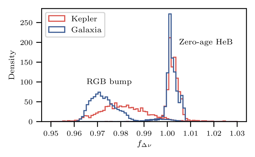
Figure 9: Distributions of the correction factor $f_{\Delta\nu}$ for stars near the RGB bump and stars near the ZAHeB edge (grey-shaded area in Fig. 4 and 7) in both Kepler (red) and Galaxia (blue) samples.

It is interesting to test whether the common model-based correction of $\Delta\nu$ proposed by Sharma et al. (2016) can reduce the scatter in the scaling relations. We calculated the departure of the $\Delta\nu$ scaling relation, $f_{\Delta\nu}$, for each star in both samples. We implemented the corrected mass $M^{\prime}=f_{\Delta\nu}^{4}M$ and radius $R^{\prime}=f_{\Delta\nu}^{2}R$ in the Kepler sample, and the corrected p-mode separation $\Delta\nu^{\prime}=f_{\Delta\nu}\Delta\nu$ in the synthetic sample.

These $\Delta\nu$ corrections made little difference to our results, for both RGB stars (Fig. 5) and HeB stars (Fig. 8). The likely explanation is that $f_{\Delta\nu}$ mainly corrects the systematic offsets in the scaling relations, which affect the location of the RGB bump and ZAHeB edge, but has a negligible influence on the intrinsic scatter of the scaling relations (Fig. 9). The standard deviation of $f_{\Delta\nu}$ for stars near the ZAHeB edge is below $0.5\%$, and that for stars near the RGB bump is about $1.0\%$.

5.4 The intrinsic scatter of the scaling relations as a function of mass and metallicity

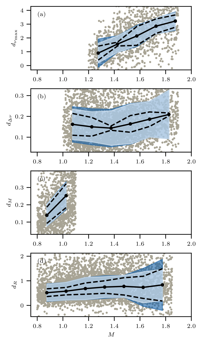
Figure 10: Distances to the ZAHeB edge as a function of stellar mass for the SYD18 sample (grey points). The solid black line traces the median values of the distances in each mass bin. The light blue show the formal uncertainties of $\Delta\nu$ and $\nu_{\rm max}$ reported by the SYD pipeline, and the dark blue regions show the intrinsic scatter of the scaling relations $\sigma_{\rm SR}$. The dashed black lines show the total scatter $\sigma_{\rm total}$.

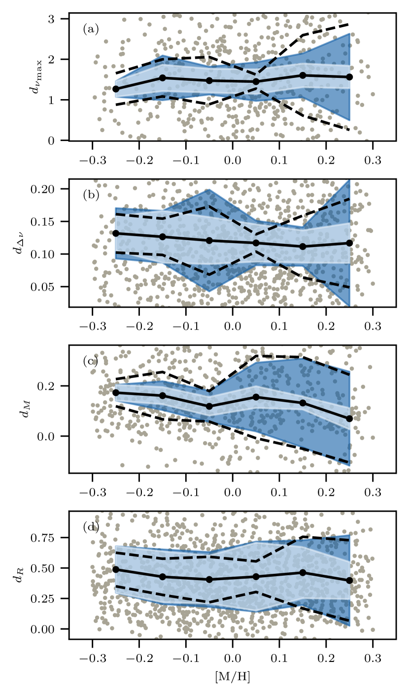
Figure 11: Similar to Fig. 10 but shown as a function of metallicity, and restricted to the APK18 sample.

We expect the intrinsic scatter in the scaling relations to be a function of stellar mass and metallicity, as we see in $f_{\Delta\nu}$. To test whether this dependence can be seen in our sample, we used HeB stars and divided both the Kepler and Galaxia samples into bins with equal widths in $M$ and [M/H], and repeated the exercise in each bin. We note that for $\Delta\nu$, $\nu_{\rm max}$ and $M$, we could only test a limited range in mass, because some points do not have vertical or horizontal distances. To study the dependence on [M/H], we used the APK18 sample instead of the SYD18 sample, because the APK18 metallicities were derived from a single instrument.

In Fig. 10 and 11 we show $\sigma_{\rm total}$ (dark blue regions) and $\sigma_{\rm SR}$ (dashed lines) as functions of $M$ and [M/H], respectively. We find no obvious change in the spread of points for $\Delta\nu$, $\nu_{\rm max}$ and $M$, possibly due to a direct consequence of the method uncertainty we claimed in section 5.1.2. The data also suggest that a higher mass and higher metallicity may result in a larger intrinsic scatter for the radius scaling relation. Whether this is a true statement can be found by populating more stars in the high mass and high metallicity region with upcoming space missions.

6 Conclusions

In this paper, we used a forward-modelling approach to match the width of the RGB bump and the sharpness of the edge formed by ZAHeB stars. Matching the broadening of those features between the Kepler and Galaxia samples allowed us to constrain the intrinsic scatter of the asteroseismic scaling relations.

The main results are summarised in Figs. 5 and 8. We found that the observed broadening arises primarily from the measurement uncertainties of $\Delta\nu$ and $\nu_{\rm max}$. By taking into account the uncertainty reported by the SYD pipeline, the scaling relations have intrinsic scatter have values of $\sim 0.5\%$ ($\Delta\nu$), $\sim 1.1\%$ ($\nu_{\rm max}$), $\sim 1.7\%$ ($M$) and $\sim 0.4\%$ ($R$). This confirms the remarkable constraining power of the scaling relations. The above numbers are appoximate, bacause the systematic uncertainties of our method arising from identifying the features is on a similar level. Although this result was obtained using stars in a limited parameter space, we expect they are applicable to a broader population spanning most low-mass red giants, provided they have similar surface properties.

Moreover, we demonstrate that using the theoretically corrected $\Delta\nu$ does not reduce the scatter by a large amount. We also found a marginal dependence of the intrinsic scatter of the radius scaling relation on mass and metallicity. However these interpretations are limited by the systematic uncertainties of our method.

Future work could include using more data from both asteroseismology and spectroscopy to allow tests in more mass and metallicity bins, especially improving the constraints for secondary clump stars. Additionally, by considering the position of those features and matching the exact distributions of stellar parameters (instead of simply the distances to the edge), one could provide constraints on physical processes such as convection and mass loss, and potentially on the offset of the scaling relations.

Data Availability

The code repository for this work is available on Github. The data sets will be shared on request to the corresponding author.

References

- Balmforth (1992) Balmforth N. J., 1992, MNRAS, 255, 603
- Belkacem et al. (2011) Belkacem K., Goupil M. J., Dupret M. A., Samadi R., Baudin F., Noels A., Mosser B., 2011, A&A, 530, A142
- Belkacem et al. (2019) Belkacem K., Kupka F., Samadi R., Grimm-Strele H., 2019, A&A, 625, A20
- Brogaard et al. (2018) Brogaard K., et al., 2018, MNRAS, 476, 3729
- Brown et al. (1991) Brown T. M., Gilliland R. L., Noyes R. W., Ramsey L. W., 1991, ApJ, 368, 599
- Cannon (1970) Cannon R. D., 1970, MNRAS, 150, 111
- Ceillier et al. (2017) Ceillier T., et al., 2017, A&A, 605, A111
- Choi et al. (2016) Choi J., Dotter A., Conroy C., Cantiello M., Paxton B., Johnson B. D., 2016, ApJ, 823, 102
- Christensen-Dalsgaard (2015) Christensen-Dalsgaard J., 2015, MNRAS, 453, 666
- Christensen-Dalsgaard et al. (2020) Christensen-Dalsgaard J., et al., 2020, A&A, 635, A165
- Dolphin (2002) Dolphin A. E., 2002, MNRAS, 332, 91
- El-Badry et al. (2019) El-Badry K., Rix H.-W., Tian H., Duchêne G., Moe M., 2019, MNRAS, 489, 5822
- Foreman-Mackey (2016) Foreman-Mackey D., 2016, The Journal of Open Source Software, 24
- Foreman-Mackey et al. (2013) Foreman-Mackey D., Hogg D. W., Lang D., Goodman J., 2013, PASP, 125, 306
- Gaulme et al. (2016) Gaulme P., et al., 2016, ApJ, 832, 121
- Geha et al. (2013) Geha M., et al., 2013, ApJ, 771, 29
- Girardi (2016) Girardi L., 2016, ARA&A, 54, 95
- Girardi et al. (2010) Girardi L., Rubele S., Kerber L., 2010, in de Grijs R., Lépine J. R. D., eds, IAU Symposium Vol. 266, Star Clusters: Basic Galactic Building Blocks Throughout Time and Space. pp 320–325 (arXiv:0910.3139), doi:10.1017/S1743921309991207
- Guggenberger et al. (2016) Guggenberger E., Hekker S., Basu S., Bellinger E., 2016, MNRAS, 460, 4277
- Hall et al. (2019) Hall O. J., et al., 2019, MNRAS, 486, 3569
- Hekker (2020) Hekker S., 2020, Frontiers in Astronomy and Space Sciences, 7, 3
- Hon et al. (2017) Hon M., Stello D., Yu J., 2017, MNRAS, 469, 4578
- Houdek et al. (1999) Houdek G., Balmforth N. J., Christensen-Dalsgaard J., Gough D. O., 1999, A&A, 351, 582
- Huber et al. (2009) Huber D., Stello D., Bedding T. R., Chaplin W. J., Arentoft T., Quirion P. O., Kjeldsen H., 2009, Communications in Asteroseismology, 160, 74
- Huber et al. (2010) Huber D., et al., 2010, ApJ, 723, 1607
- Huber et al. (2017) Huber D., et al., 2017, ApJ, 844, 102
- Hunter (2007) Hunter J. D., 2007, Computing in Science & Engineering, 9, 90
- Iben (1968) Iben I., 1968, Nature, 220, 143
- Jiménez et al. (2011) Jiménez A., García R. A., Pallé P. L., 2011, ApJ, 743, 99
- Jiménez et al. (2015) Jiménez A., García R. A., Pérez Hernández F., Mathur S., 2015, A&A, 583, A74
- Kallinger et al. (2010a) Kallinger T., et al., 2010a, A&A, 509, A77
- Kallinger et al. (2010b) Kallinger T., et al., 2010b, A&A, 522, A1
- Khan et al. (2018) Khan S., Hall O. J., Miglio A., Davies G. R., Mosser B., Girardi L., Montalbán J., 2018, ApJ, 859, 156
- Khan et al. (2019) Khan S., et al., 2019, A&A, 628, A35
- King et al. (1985) King C. R., Da Costa G. S., Demarque P., 1985, ApJ, 299, 674
- Kjeldsen & Bedding (1995) Kjeldsen H., Bedding T. R., 1995, A&A, 293, 87
- Marigo et al. (2017) Marigo P., et al., 2017, ApJ, 835, 77
- Miglio et al. (2012) Miglio A., et al., 2012, MNRAS, 419, 2077
- Mosser et al. (2010) Mosser B., et al., 2010, A&A, 517, A22
- Mosser et al. (2012) Mosser B., et al., 2012, A&A, 548, A10
- Pinsonneault et al. (2018) Pinsonneault M. H., et al., 2018, ApJS, 239, 32
- Refsdal & Weigert (1970) Refsdal S., Weigert A., 1970, A&A, 6, 426
- Reimers (1975) Reimers D., 1975, Memoires of the Societe Royale des Sciences de Liege, 8, 369
- Rodrigues et al. (2017) Rodrigues T. S., et al., 2017, MNRAS, 467, 1433
- Sahlholdt & Silva Aguirre (2018) Sahlholdt C. L., Silva Aguirre V., 2018, MNRAS, 481, L125
- Serenelli et al. (2017) Serenelli A., et al., 2017, ApJS, 233, 23
- Sharma et al. (2011) Sharma S., Bland-Hawthorn J., Johnston K. V., Binney J., 2011, ApJ, 730, 3
- Sharma et al. (2016) Sharma S., Stello D., Bland-Hawthorn J., Huber D., Bedding T. R., 2016, ApJ, 822, 15
- Sharma et al. (2019) Sharma S., et al., 2019, MNRAS, 490, 5335
- Silva Aguirre et al. (2012) Silva Aguirre V., et al., 2012, ApJ, 757, 99
- Stello et al. (2008) Stello D., Bruntt H., Preston H., Buzasi D., 2008, ApJ, 674, L53
- Stello et al. (2016) Stello D., Cantiello M., Fuller J., Garcia R. A., Huber D., 2016, Publ. Astron. Soc. Australia, 33, e011
- Ulrich (1986) Ulrich R. K., 1986, ApJ, 306, L37
- Viani et al. (2017) Viani L. S., Basu S., Chaplin W. J., Davies G. R., Elsworth Y., 2017, ApJ, 843, 11
- Virtanen et al. (2020) Virtanen P., et al., 2020, Nature Methods, 17, 261
- White et al. (2011) White T. R., Bedding T. R., Stello D., Christensen-Dalsgaard J., Huber D., Kjeldsen H., 2011, ApJ, 743, 161
- Yıldız et al. (2016) Yıldız M., Çelik Orhan Z., Kayhan C., 2016, MNRAS, 462, 1577
- Yu et al. (2018) Yu J., Huber D., Bedding T. R., Stello D., Hon M., Murphy S. J., Khanna S., 2018, ApJS, 236, 42
- Zhou et al. (2019) Zhou Y., Asplund M., Collet R., 2019, ApJ, 880, 13
- Zinn et al. (2019) Zinn J. C., Pinsonneault M. H., Huber D., Stello D., Stassun K., Serenelli A., 2019, ApJ, 885, 166
- van der Walt et al. (2011) van der Walt S., Colbert S. C., Varoquaux G., 2011, Computing in Science Engineering, 13, 22