Anisotropic solid dark energy
Abstract
In this paper, we study a triad of inhomogeneous scalar fields, known as “solid”, as a source of homogeneous but anisotropic dark energy. By using a dynamical system approach, we find that anisotropic accelerated solutions can be realized as attractor points for suitable choices of the parameters of the model. We complement the dynamical analysis with a numerical solution whose initial conditions are set in the deep radiation epoch. The model can give an account of a non-negligible spatial shear within the observational bounds nowadays, even when the later is set to zero at early times. However, we find that there is a particular region in the parameter space of the model in which the Universe isotropizes. The anisotropic attractors, the particular isotropic region, and a nearly constant equation of state of dark energy very close to are key features of this scenario. Following a similar approach, we also analyzed the full isotropic version of the model. We find that the solid can be characterized by a constant equation of state and thus being able to simulate the behavior of a cosmological constant.
pacs:
98.80.Cq; 95.36.+xI Introduction
The current Universe is expanding at an accelerated rate. This fact was first discovered in type Ia supernovae (SNe Ia) surveys Riess et al. (1998); Schmidt et al. (1998); Perlmutter et al. (1999) and later confirmed by several other observations like large scale structures (LSS) Tegmark et al. (2004, 2006), cosmic microwave background (CMB) Spergel et al. (2003); Ade et al. (2016a), and baryon acoustic oscillations (BAO)Percival et al. (2007); Aubourg et al. (2015) measurements. Observations also show that our expanding Universe is highly homogeneous, isotropic and spatially flat at cosmological scales de Bernardis et al. (2000); Jaffe et al. (2003); Aghanim et al. (2020). The simplest description of the Universe is based on the standard Cold Dark Matter (CDM) model. In this model, the current accelerated expansion of the Universe is due to the repulsive effect of a constant energy density with negative pressure, which is given by the cosmological constant Amendola and Tsujikawa (2015); Bamba et al. (2012). Despite its success, there are several theoretical and observational problems with this scenario. One of the theoretical difficulties is the so-called cosmological constant problem, which asserts that if is associated with the vacuum energy density of the Universe, the value predicted by the theory and the value obtained from observations differs by several tens orders of magnitude Weinberg (1989); Martin (2012). On the observational side, the tension states that the current value of the Hubble parameter calculated from the CMB data does not agree with the value computed from local measurements of SNe Ia Riess et al. (2016, 2019). It seems that this tension could be alleviated if extensions to CDM model are considered Di Valentino et al. (2017); Guo et al. (2019); Agrawal et al. (2019).
The search for alternatives to the standard model is generally split into two broad categories: modified gravity theories and dynamical dark energy. While the former has been recently under observational pressure Collett et al. (2018); Ezquiaga and Zumalacárregui (2018); He et al. (2018); Do et al. (2019); Abbott et al. (2019), the latter is usually based on time-dependent fields with vanishing spatial gradients Copeland et al. (2006); Yoo and Watanabe (2012). This choice ensures that the background geometry can be described by a homogeneous and isotropic metric, and thus the evolution of the Universe is also homogeneous and isotropic. On the other hand, some observations seem to imply a violation of the Universe’s isotropy at large scales—the so called CMB anomalies Perivolaropoulos (2014); Schwarz et al. (2016); Akrami et al. (2020a)—suggesting that background metrics different to the homogeneous and isotropic Friedmann-Lemaître-Robertson-Walker (FLRW) metric should be considered Bennett et al. (2011); Akrami et al. (2020b, a). It has been also pointed out that some of these CMB anomalies could be explained by the introduction of an anisotropic late-time accelerated expansion Battye and Moss (2009); Perivolaropoulos (2014); Schwarz et al. (2016).
An anisotropic dark energy can be realized by considering a homogeneous but spatially anisotropic metric, together with a suitable arrangement of the fields driving the expansion of the universe. Among the proposals for anisotropic dark energy, we can find models of vector fields Koivisto and Mota (2008a, b); Thorsrud et al. (2012), p-forms Beltrán-Almeida et al. (2019); Guarnizo et al. (2019); Beltrán-Almeida et al. (2020) or non-Abelian gauge fields Orjuela-Quintana et al. (2020); Guarnizo et al. (2020). All of these models are based on time-dependent fields, so as to comply with the homogeneity of the background metric. Nonetheless, in Refs. Armendariz-Picon (2007); Endlich et al. (2013), it was shown that a triad of scalar fields with spatially constant but nonzero gradients can generate a homogeneous and isotropic energy-momentum tensor, i.e. invariant under translations and spatial rotations. This triad, known as “solid”, is given by
| (1) |
where is a scalar field and is a comoving cartesian coordinate. The solid configuration for inhomogeneous scalar fields is similar to other configurations for different fields. For instance, the cosmic triad for vector and nonabelian gauge vector fields Bento et al. (1993); Armendariz-Picon (2004); Golovnev et al. (2008); Maleknejad and Sheikh-Jabbari (2013); Mehrabi et al. (2017), the U(1) triad of homogeneous scalar fields Firouzjahi et al. (2019), and the recent Higgs triad Orjuela-Quintana et al. (2020), among others.
In Refs. Armendariz-Picon (2007), an isotropic energy-momentum tensor is achieved since the Lagrangians constructed from each of the three scalar fields are equal, while in Ref. Endlich et al. (2013) it is assumed that the scalar fields possess an internal SO(3) symmetry such that the ansatz in Eq. (1) is invariant under combined spatial and internal rotations. In Refs. Bartolo et al. (2013, 2014), it was shown that the solid configuration in Eq. (1) can support prolonged anisotropic inflationary solutions111Other scenarios of anisotropic inflation have been studied, see for instance Kanno et al. (2008, 2008, 2008); Yokoyama and Soda (2008); Watanabe et al. (2009, 2010); Yamamoto et al. (2012); Soda (2012); Ohashi et al. (2013).. In this work, we show that this characteristic behavior is also present at late-times for most of the parameter space of the model and thus the final stage of the Universe can be an anisotropic accelerated expansion, even if the initial spatial shear is set to zero. Nonetheless, there is a particular region in the parameter space of the model where the Universe becomes isotropic, meaning that the solid does not source the shear, which then eventually vanishes. For completeness, we also show that dark energy dominance is possible when the background metric is homogeneous and isotropic.
This paper is organized in the following way. In Sec. II, we present the action and the energy-momentum tensor of the model. In Sec. III, the equations of motion in an homogeneous but anisotropic background are derived. Section IV is dedicated to the dynamical analysis of the model. A numerical integration of the background equations and the general cosmological evolution is presented in Sec. V. The isotropic version of the model is treated in Sec. VI. Finally, our conclusions are presented in Sec. VII.
II General Model
At this point, it is worth emphasizing that what we call a “solid” is the specific configuration of three inhomogeneous scalar fields given by Eq. (1).222Even more general configurations can be studied, like the “supersolids” in Ref. Celoria et al. (2017). However, different dynamics of the solid can be studied depending on the particular action constructed with the fields (1). For example, in Ref. Endlich et al. (2013), it is assumed that the solid itself is equipped with an internal SO(3) symmetry and its Lagrangian is a function of SO(3) invariants constructed from the matrix , being the Lagrangian compatible with a FLRW geometry. This same Lagrangian was studied in Refs. Bartolo et al. (2013, 2014) but in an anisotropic background, where it was shown that prolonged anisotropic inflationary solutions can be obtained. Four our purposes, the assumption of an internal SO(3) symmetry is not necessary, and we thus opt for studying the simpler action
| (2) |
where is the reduced Planck mass, is the Ricci scalar, is the Lagrangian characterizing the dynamics of the scalar field , whose argument is the canonical kinetic-type term
| (3) |
and and are the Lagrangians for matter and radiation fluids, respectively. This action is an extension to the late-time cosmology of the model studied in Ref. Armendariz-Picon (2007) in the inflationary context.
Varying the action in Eq. (2) with respect to the space-time metric , we get the gravitational field equations , with the Einstein tensor and the total energy tensor given by
| (4) |
where and are the energy tensors associated to the matter and radiation perfect fluids, respectively, and we have used the shorthand notation . Varying the action with respect to , we get the equation of motion
| (5) |
III Background Equations of Motion
Since we are interested in anisotropic deformations sourced by the solid, we adopt the geometry of a homogeneous but anisotropic Bianchi-I metric. For simplicity, we assume that there exists a residual isotropy in the plane, such that the background geometry is given by
| (6) |
where is the average scale factor and is the geometrical shear, being both functions of the cosmic time . In Ref. Armendariz-Picon (2007), it was shown that the action in Eq. (2) can be compatible with the symmetries of the FLRW metric if the three Lagrangians are identical; i.e. and thus . However, in the Bianchi-I background in Eq. (6), the canonical kinetic-type terms read
| (7) |
and the requirement for the Lagrangians in this case is
| (8) |
Considering the “” component of the gravitational field equations, the first “Friedman” equation reads
| (9) |
where is the Hubble parameter,333Here, an overdot denotes a derivative with respect to the cosmic time . and we have defined and as the densities for the matter and radiation perfect fluids, respectively. The second Friedman equation follows from , which can be written as
| (10) |
Finally, the evolution equation for the geometrical shear is obtained from the relation as
| (11) |
Since we are interested in anisotropic late-time accelerated solutions, it is necessary to characterize the dark energy fluid. We define the density and pressure of dark energy by
where we have defined the quantities
| (12) |
which characterize the form of the Lagrangians and , respectively.
Note that our choice to include the geometrical shear in and (instead of considering only the contribution coming from the solid) allows us to write the continuity equation simply as
| (13) |
which greatly simplifies our analysis.444Had we chosen to separate the contributions of the solid and the geometry, we would end up with an equation of the form , where is the time derivative of the spatial part of the metric, and is the trace-free part of the energy-momentum tensor.
IV Dynamical system
IV.1 Autonomous System
In order to proceed, we introduce the following dimensionless variables
| (14) |
such that the first Friedman equation (9) becomes the constraint
| (15) |
Changing the cosmic time for the number of -folds defined as , the background equations (9)-(11) are replaced by the autonomous system555Here, a prime denotes a derivative with respect to the number of -folds .
| (16) | ||||
| (17) | ||||
| (18) | ||||
| (19) |
where the deceleration parameter, , is given by
| (20) |
However, instead of the deceleration parameter, we equivalently characterize the evolution of the average scale factor in terms of the effective equation of state .
The dark sector is characterized by its equation of state , which in terms of the dynamical variables reads
| (21) |
and its density parameter .
Since the functions and cannot themselves be expressed in terms of the dimensionless variables, it is necessary to choose the specific Lagrangians and in order to get a closed autonomous system. In this case, the simplest model is obtained when and are constants, which corresponds to a power law model
such that
| (22) |
We want to stress that a different choice would yield to time-dependent parameters and , such that, in principle, the equation of state of dark energy could vary in unimagined ways. Due to the lacking of restrictions in the functional form of the Lagrangians (some of them could be obtained from a reconstruction method, for example), we focus in this particular choice by its simplicity. In the next subsection, we will study the asymptotic behavior of the system by finding the fixed points of the autonomous system, and we will see that this simple choice is enough to get interesting behaviors.
IV.2 Fixed Points and Stability
In the following, we discuss the fixed points relevant to the radiation (), matter (), and dark energy eras (), which can be obtained by setting , , , and in equations (16)-(19). The stability of these points can be known by perturbing the autonomous set around them. Up to linear order, the perturbations satisfy the differential equation,
| (23) |
where is a Jacobian matrix. The sign of the real part of the eigenvalues of determines the stability of the point. A fixed point is an attractor, or sink, if the real part of all the eigenvalues are negative. If at least one of the eigenvalues has positive real part it is called a saddle. If the real part of all the eigenvalues are positive the fixed point is called a repeller or source.
In what follows, we refer to each point by its name, which is defined as , or – depending on wheter it corresponds to a radiation, matter or dark energy dominated universe – followed by a number. The points and their eigenvalues are gathered in Tables 1 and 2, respectively.
| Fixed Point | stability | ||||||
|---|---|---|---|---|---|---|---|
| R-1 | 0 | 0 | 1 | 0 | 0 | 1/3 | saddle |
| R-2 | 0 | 0 | 1/3 | saddle | |||
| R-3 | 0 | 0 | 1/3 | saddle | |||
| M-1 | 0 | 0 | 0 | 1 | 0 | 0 | saddle/attractor |
| M-2 | 0 | 0 | 0 | saddle/attractor | |||
| M-3 | 0 | 0 | 0 | saddle/attractor | |||
| DE-1 | 0 | 0 | saddle/attractor | ||||
| DE-2 | 0 | 0 | 0 | saddle/attractor | |||
| DE-3 | 0 | 0 | saddle/attractor |
| Fixed Point | ||||
|---|---|---|---|---|
| R-1 | ||||
| R-2 | ||||
| R-3 | ||||
| M-1 | ||||
| M-2 | ||||
| M-3 | ||||
| DE-1 | ||||
| DE-2 | ||||
| DE-3 | too long to show | |||
IV.2.1 Radiation Dominance
(-1) Isotropic radiation:
This point corresponds to an isotropic radiation-dominated universe, and it trivially satisfies the constraint (15). One can check that the eigenvector associated with the eigenvalue points in the direction in the phase space , indicating that the trajectories around this point are attracted in this direction. This means that the shear decays from its value around this point. On the other hand, the eigenvector associated with the eigenvalue points to the direction, meaning that radiation is running away from its value . The eigenvalues and are positive for and less than 2, respectively. Under this condition, (R-1) is a saddle with three positive eigenvalues, and the dark components and grow during the radiation epoch, since the eigenvectors associated to these eigenvalues () point to the and directions, respectively.
(-2) Anisotropic radiation scaling with :
This corresponds to an anisotropic solution where the density parameter and equation of state of dark energy are given by
| (24) |
indicating that dark energy scales as a radiation fluid, or “dark radiation”. This point is a viable solution if the conditions
are satisfied. Furthermore, the big-bang nucleosynthesis (BBN) gives the bound Bean et al. (2001). Imposing all of these conditions, we determine that the physical region of existence of the point (R-2) is
| (25) |
The eigenvalues of in this point (see Table 2) tell us that this is a saddle point. The eigenvalues and are negative in the region of existence given in Eq. (25). The second eigenvalue is positive in the region of existence of the point for , and negative otherwise. Since the eigenvector associated to this eigenvalue points to the direction when , the dark component grows during the radiation epoch.
(-3) Anisotropic radiation scaling with :
The density parameter and equation of state of dark energy in this solution are given by
| (26) |
Imposing the conditions
as well as the BBN bound , the physical region of existence of (R-3) becomes
| (27) |
The eigenvalues of in this point show that this is a saddle point. The eigenvalues and are negative in the region of existence given in Eq. (27). The second eigenvalue is positive in the region of existence of the point for , and negative otherwise. Since the eigenvector associated to this eigenvalue points to the direction, when , the dark component grows during the radiation epoch.
IV.2.2 Matter Dominance
(-1) Isotropic matter:
This corresponds to an isotropic matter-dominated universe with
, and undetermined. The eigenvector associated with the eigenvalue points to the direction indicating that the trajectories around this point are attracted in this direction (faster than around the point (R-1)). In this case, the eigenvector associated with the eigenvalues points to the direction, meaning that radiation is decaying. The eigenvalues and are positive for and less than , respectively. Under this condition, (M-1) is a saddle with two positive eigenvalues, and the dark components and grow during the matter epoch, since the eigenvector associated to these eigenvalues point to the and directions, respectively.
(-2) Anisotropic matter scaling with :
The energy-density and equation of state of dark energy in this solution are given by
| (28) |
indicating that scales as a pressureless fluid. This point is a viable solution if
are satisfied. Moreover, CMB anisotropies give the bound around the redshift Aghanim et al. (2020) (which ensures that we are deep in the matter-dominated era). Therefore, the physical region of existence of (M-2) is
| (29) |
The eigenvalues and are negative in the region of existence given in Eq. (29). For this point to be a possible candidate for the matter-dominated epoch, it has to be a saddle rather than an attractor in order to allow a subsequent accelerated expansion epoch. This means that the second eigenvalue has to be positive. We have in the region of existence of the point for . Since the eigenvector associated to this eigenvalue points to the direction, when , the dark component grows during the matter epoch.
(-3) Anisotropic matter scaling with :
For this point, the energy-density and equation of dark energy are
| (30) |
Imposing the conditions
together with the CMB bound , the physical region of existence of (M-2) is found to be
| (31) |
The eigenvalues and are negative in the region of existence given in Eq. (31). For this point to be a saddle, the second eigenvalue has to be positive, which is the case in its region of existence if . Since the eigenvector associated to this eigenvalue points to the direction, when , the dark component grows during the matter epoch.
IV.2.3 Dark Energy Dominance
(-1) Anisotropic dark energy scaling with :
This is the first solution corresponding to an anisotropic dark energy dominated universe. The energy density and equation of state of dark energy are given by
| (32) |
If we now impose the conditions and – the latter being necessary for having accelerated solutions666We concentrate in no-ghost solutions; i.e. , although this possibility has not been discarded by observations yet Aghanim et al. (2020). – we find the following regions of existence777The symbol stands for the logic “OR”.
| (33) |
However, since current observations favour an equation of state of dark energy nowadays Aghanim et al. (2020), and a small anisotropy888Here, the subscript means that the corresponding quantity is evaluated nowadays. Campanelli et al. (2011); Amirhashchi and Amirhashchi (2020), we take the region of existence of this point as
| (34) |
The first branch in (33), although leading to a viable equation of state for dark energy, leads to a too large , and is thus discarded. Note that if , then given that the Lagrangian becomes a cosmological constant.
(-2) Anisotropic dark energy with :
The dark energy parameters in this solution are
| (36) |
Imposing the conditions and , we arrive at the following region of existence
| (37) |
Note that if , then given that the Lagrangian becomes a cosmological constant.
(-3) Anisotropic dark energy scaling with and :
This is the only solution in which dark energy scales with both and . The parameters of dark energy in this case are
| (39) |
By demanding that both and are positive, and that , we arrive at two possible regions for the parameters and :999The symbol stands for the logic “AND”.
| (40) | ||||
| (41) |
These regions are plotted in Fig. 1. Notice that the cases and are not allowed in the region of existence.
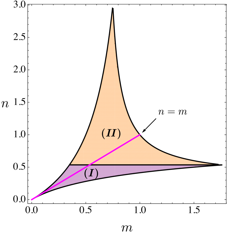
Note that in the region of existence of (-3) there is the possibility that (magenta line in Fig. 1), implying that , as it can be seen in Table 1. This follows since, in the case , (see Table 1) and therefore by the definition of the variables. This implies that the right-hand side of Eq. (11) is zero, and thus the shear decays since the solid is not sourcing it. In other words, the shear is dynamically erased given that the Lagrangians behave in the same way. On the other hand, and as we will see later, the shear grows at late-times even if it is set to zero as the initial condition, since the solid sources it given that the Lagrangians behave in different ways, i.e. when .
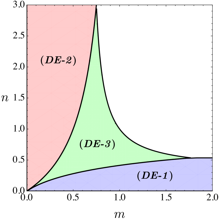
The eigenvalues of in this fixed point are given by too long algebraic expressions involving the parameters and . We omit them here since only the sign of the real part of the eigenvalues is relevant to the stability analysis. We investigated the parameter window, inside the regions of existence in Fig. 1, where are negative, and we found that the four eigenvalues are negative inside the whole region of existence of the point; i.e. when (DE-3) exists, it is an attractor.
From the previous analysis, it is clear that the three dark energy dominated points can be attractors. In Fig. 2, we plot the parameter space where each dark energy dominated point is an attractor. We can see that these regions are separated by bifurcation curves (black solid lines), meaning that they are mutually excluded. This ensures that the system has only one dark energy attractor for a particular set of parameters . This leave the case as the only possibility to get an isotropic Universe, since the points (-1) and (-2) are saddle while (-3) is the global attractor under this condition.
V Cosmological evolution
Figure 2 summarizes our main results regarding the theoretical viability of the solid as a model of anisotropic dark energy. In this section we want to study the dynamics of the model for the parameters inside the coloured regions of Fig. 2. We will implicitly assume that, prior to the radiation epoch, the Universe underwent an inflationary period which perfectly smoothed any initial spatial shear or inhomogeneities. Therefore, we choose as an initial condition101010Here, the subscript means that the corresponding quantity is evaluated at some time deep in the radiation epoch., such that the starting point for any cosmological trajectory is from the isotropic radiation point (R-1). Moreover, we will choose parameters and such that the attractor point is given by (DE-2). This choice allows us to give a simple and concrete example of the cosmological dynamics which can be easily extended to the other attractor points. Since , it is natural to assume that the contributions to the energy budget coming from the variables and are the same at the starting point. Having this in mind, we have chosen
| (42) |
as initial conditions at the redshift , and we have integrated the system up to . Since observations favor an equation of state of dark energy close to , from Eq. (36) we have to choose . In particular, we have chosen . From Fig. 2, we can see that there are less restrictions regarding the choice of the parameter . For example, we could assume a value for allowing the existence of the scaling points (R-2) or (M-2). However, for simplicity, we have chosen , such that the scaling points do not exist.
In Fig. 3, we plot the dynamical evolution of , , , and obtained from the numerical integration of Eqs. (16)-(19). In the case where , there are no appreciable changes in the cosmological behavior presented in Fig. 3. However, a “stiff matter” epoch driven by the spatial shear appears before the radiation era, which we briefly treat in Appendix A.
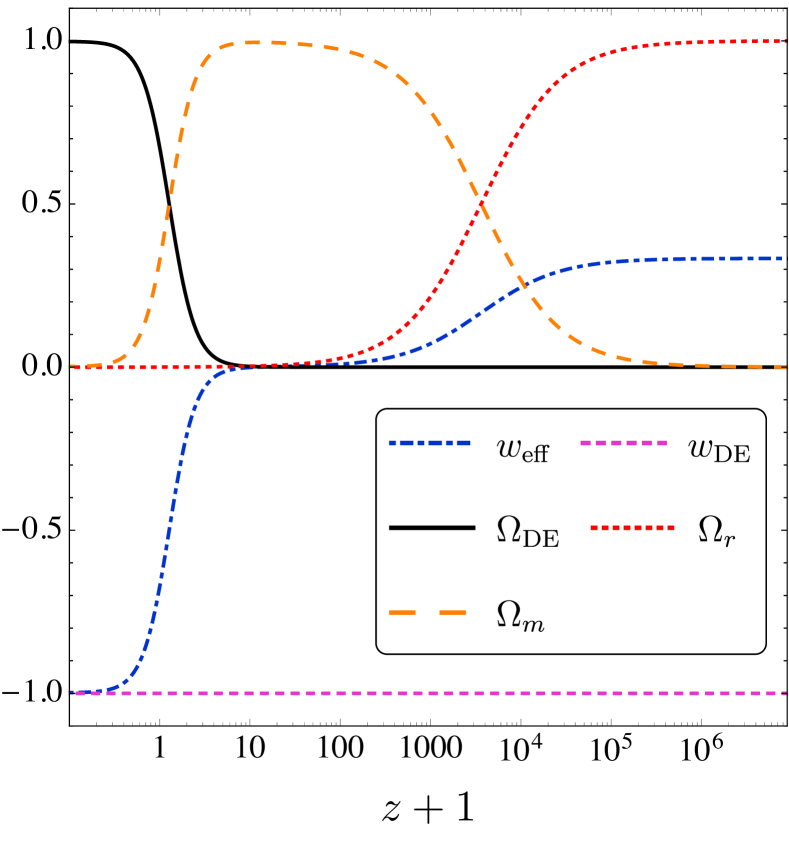
In particular, Fig. 3 shows that the radiation-dominated epoch ( and ) runs from to where the radiation-matter transition occurs. Moreover, during this transition, obeying the BBN constraint Bean et al. (2001). The length of this radiation phase is in agreement with the constraint given in Ref. Álvarez et al. (2019). From , the Universe is dust-dominated ( and ) until at the matter-dark energy transition. The contribution of the dark sector is at , value which is within the CMB bound Ade et al. (2016b). The dark energy-dominance ( and ) starts from and on into the future, agreeing with the results given by the dynamical system analysis, i.e. (DE-2) is an attractor. This is further supported by the fact that the values of and are those predicted by the dynamical system. Explicitly, , , , and in the far future (), which are consistent with the values computed from the (DE-2) line in Table 1 and Eq. (36). Although seems to be constant during the whole expansion history, this is not the case. Indeed, during the radiation-matter transition () we have , while during the matter-dark energy transition () we have . The final value is , which corresponds to the value in the attractor point [see Eq. (36)]. Thus, the numerical solution shows a nearly constant varying equation of state of the dark energy, changing only about during this particular cosmological trajectory. This tiny variation in is impossible to verify by current technology, since it is well below the threshold of missions like Planck or Euclid Aghanim et al. (2020); Laureijs et al. (2011).
From Fig. 3, we can also notice that dark energy does not behave as radiation or dust, given that , confirming that the Universe does not approach the scaling anisotropic points. Indeed, we have confirmed, for several pairs of parameters , that the expansion history of the Universe is very similar to that shown in Fig. 3, and thus the cosmological trajectories of the Universe are never close to the scaling anisotropic points. We can thus conclude that the typical cosmological evolution is given by
where can be 1, 2 or 3, depending on the and values we choose (see Fig. 2).
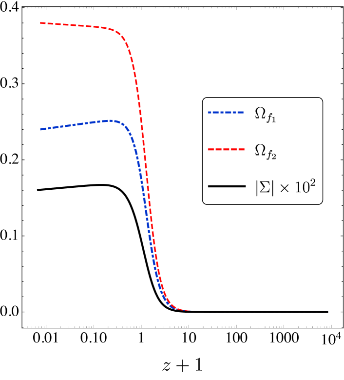
As shown in Fig. 4, The density parameters and associated with each solid Lagrangian grow during the late matter-dominated epoch around , while they are subdominant in the whole prior cosmological evolution, as expected from the dynamical analysis.
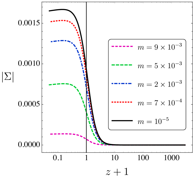
We have also investigated the evolution of taking the same initial conditions in Eq. (42) and , but this time with different choices for the parameter in such a way that (DE-2) is the only attractor of the system. The results are shown in Fig. 5, where we can see that starts to grow around , similarly to and as seen in Fig. 4. The values predicted for the present spatial shear are , corresponding to the black solid curve in Fig. 5, which are in agreement with the observational bounds Campanelli et al. (2011); Amirhashchi and Amirhashchi (2020). We want to stress that, even for , the final state of the Universe is an anisotropic accelerated expansion.
On the other hand, we corroborated that the other two dark energy points, namely (DE-1) and (DE-3), can be attractors in their respective stability regions (see Fig. 2). In order for (DE-1) to be the only attractor of the system, we choose and according to the existence and stability conditions in Eqs. (34) and (35). The initial conditions are the same as in Eq. (42) and, although the values of and change, the cosmological evolution is qualitatively the same. In particular, the shear and the equation of state of dark energy today are and . We confirm that the values predicted by the dynamical system analysis are in agreement with our numerical solution: and [see Table 1 and Eq. (32)], when evaluated for redshifts . Finally, for the point (DE-3), we choose and , so that this point is the only attractor of the system. Using the same initial conditions as in Eq. (42), the cosmological dynamics is not significantly changed apart from the important fact that during the whole cosmological evolution, i.e. the expansion history is isotropic. By changing the values of the parameters and while keeping (DE-3) as the only attractor, we verified that the case is the unique isotropic solution as expected from the discussion in Sec. IV.2.3. The numerical results are also consistent with the analytical findings, namely: and for redshifts [see Table 1 and Eq. (39)], i.e. the attractor point is reached very quickly.
V.1 Observational Signatures
From the magnitude-redshift data of SNe Ia, the analysis of Ref. Campanelli et al. (2011) showed that the present value of the spatial shear is constrained to be . More recently, the authors of Ref. Amirhashchi and Amirhashchi (2020) used a combination of the observational Hubble data and SNe Ia measurements to put the tighter bound of . Similarly, future weak-lensing measurements with the Euclid satellite are expected to reach a similar sensitivity level of Pereira et al. (2016). For the set of parameters and initial conditions used in Fig. 5, we can see that is within these bounds, although it can take greater values in the future cosmological evolution.
An anisotropic dark energy has the potential for breaking of statistical isotropy and explain of some of the large scale CMB anomalies. In particular, anisotropic pressure can induce peculiar velocity flows, anisotropy in the SNe Ia data, and significant CMB dipole and quadrupole Perivolaropoulos (2014) fluctuations. The main observational effect of an anisotropic shear is its contribution to the CMB temperature anisotropies. This contribution is introduced through the redshift at last scattering surface, which becomes anisotropic. Considering only large-scale fluctuations, this can be quantified as Appleby et al. (2010); Beltrán-Almeida et al. (2019):
| (43) |
where is the CMB temperature anisotropies, is the unit vector along the line-of-sight, and is the value of the geometrical shear at the time of decoupling (). Since , we can obtain the values for the geometrical shear by numerical integration. For the cases with the largest and smallest shear today, as depicted in Fig. 5, and using the same initial conditions of Eq. (42), we obtain
| (44) | |||
| (45) |
which are in qualitative agreement with the conservative bound Aghanim et al. (2020), thus, a solid anisotropic dark energy could alleviate the observed CMB quadrupole anomaly.
VI Isotropic Dark Energy
So far, we have been mainly interested in the solid as a viable model for an anisotropic late-time expansion of the Universe. Interestingly, in the previous analysis, we showed that the only possibility to get an isotropic Universe is the case when . Nonetheless, the solid is also compatible with the FLRW metric, and it can also be used to describe an isotropic late-time expansion with equation of state close to . For this we have to consider that the Lagrangians are identical. Thus, the isotropic model requires in the Bianchi-I metric in Eq. (6), and:
| (46) |
Defining and using the density parameter in Eq. (14), the autonomous set is reduced to
| (49) | ||||
| (50) |
where is given in terms of and by the Friedman constraint coming from Eq. (47), and the deceleration parameter is given by
| (51) |
where is a function characterizing the form of the Lagrangian . Assuming a power law model, , we get and the system is closed. Three fixed points can be found: a radiation dominated point which is a source for , a matter dominated point which is a saddle for , and a dark energy dominated point which is an attractor for .
In Fig. 6, we numerically integrate the set given by Eqs. (49) and (50). We assume and the initial conditions according with the present observed values for the density parameters: Aghanim et al. (2020):
| (52) |
We can see that the cosmological evolution is quite similar to the one of the anisotropic case, which is shown in Fig. 3 and detailed in Sec. V.

In contrast to the quintessence model, this model does not have a kination epoch previous to the radiation domination period. This is due to the fact that the kination epoch requires , where is the quintessence scalar field and its potential. In the quintessence model, the potential is necessary in order to get accelerated expansion since this stage is provided by . In the present case, such potential is not needed since the accelerated expansion is driven by the proper kinetic terms of the scalar fields through the function . Another important difference between this model and quintessence is that the equation of state of dark energy can be constant or dynamical. The equation of state of dark energy is
| (53) |
which is constant for constant (power law model), thus mimicking a cosmological constant. However, can also be dynamical for a general time-dependent function.
VII Conclusions
In this work we studied a set of three scalar fields with a constant but nonvanishing spatial gradients as a source of anisotropic dark energy. This particular set of inhomogeneous scalar fields, known as “solid”, has been used in the inflationary context showing interesting features at the perturbative level Armendariz-Picon (2007); Endlich et al. (2013). It was also shown that anisotropic inflationary solutions are possible Bartolo et al. (2013, 2014). Here, we have investigated the late-time dynamics of the solid in a Bianchi-I expanding universe. Through a dynamical system analysis, we showed that for a particular power-law model, the solid can generate an anisotropic late-time accelerated expansion, being this epoch an attractor of the system for suitable values of the free parameters of the model (see Fig. 2). In these regions, the cosmological evolution starts in a radiation-dominance epoch, followed by a matter-dominance epoch, and ending in a possible anisotropic dark energy-dominated period which can be realized by three different points, whose attractor regions are separated by bifurcation curves, i.e. they are mutually excluded. Nonetheless, we found that in the particular case when the Universe isotropizes provided that the Lagrangians evolve in the same way.
The dynamical analysis was complemented with a numerical integration of the dynamical system. The parameters were fixed in such a way that (DE-2) was the only attractor point and the equation of state of dark energy was close to as expected from observations Aghanim et al. (2020). The initial conditions were chosen in the deep radiation era (redshift ) and assuming a zero spatial shear (). We found that the spatial shear differs sensibly from zero at around , taking nonnegligible values nowadays but within the observational bounds Campanelli et al. (2011); Amirhashchi and Amirhashchi (2020). The numerical solution also showed a nearly constant equation of state of dark energy, , that only changed about from its value at to its final value in the far future (). We verified that similar behaviors are obtained if the parameters are chosen to establish (DE-1) or (DE-3) as the attractor points.
The nonvanishing shear after the radiation-dominated epoch leaves imprints on CMB and SNe Ia data. In particular, the shear affects the CMB quadrupole temperature anisotropy through the standard Sachs-Wolfe formula. We showed that the change of the spatial shear from decoupling to today can be compatible with the CMB quadrupole data. In particular, if is of order , there may be an interesting possibility for addressing the CMB quadrupole anomaly.
We have also investigated the isotropic version of the solid model as a candidate for (isotropic) dark energy. In this case, only three fixed points were found: a source radiation point, a saddle matter point, and an attractor dark energy point. The evolution of the Universe is very similar to the anisotropic case (see Figs. 3). However, for a power-law model, the equation of state of dark energy is indeed a constant [see Eq. (53)], and is thus phenomenologically distinguishable from quintessential models.
Acknowledgements
This work was supported by the following grants: Vicerrectoría de Investigaciones Universidad del Valle Grant No. 71220 and Patrimonio Autónomo - Fondo Nacional de Financiamiento para la Ciencia, la Tecnología y la Innovación Francisco José de Caldas (MINCIENCIAS - COLOMBIA) Grant No. 110685269447 RC-80740-465-2020, project 69723 T.S.P thanks Brazilian funding agencies CAPES and CNPq (grants 438689/2018-6 and 311527/2018-3) for the financial support.
Appendix A Other fixed point
The fixed points presented are the relevant point for the cosmological history of the Universe. Nonetheless, the dynamical system has another fixed points, which we present here.
() Stiff matter domination:
This fixed point is characterized by
| (54) |
with , and . Since , these points correspond to a “stiff matter” domination driven by the spatial shear . This also implies that the energy density of dark energy decays as , and thus this period is prior to the radiation domination. Although these points are the only possible sources of the model (i.e., all the eigenvalues of the Jacobian matrix are positive), they can be arbitrarily pushed back to the past depending on how small is. For example, these points are in the infinite past for . This stiff fluid is common in quintessence models where the kinetic term of the scalar field has the chance to dominate Amendola and Tsujikawa (2015), and it has been pointed out in some works that this period can be useful in the study of the reheating process Ferreira and Joyce (1998); Pallis (2006); Dimopoulos and Markkanen (2018); Bettoni et al. (2019); Bettoni and Rubio (2018, 2020).
References
- Riess et al. (1998) A. G. Riess et al. (Supernova Search Team), “Observational evidence from supernovae for an accelerating universe and a cosmological constant,” Astron. J. 116, 1009–1038 (1998), arXiv:astro-ph/9805201 .
- Schmidt et al. (1998) B. P. Schmidt et al. (Supernova Search Team), “The High Z supernova search: Measuring cosmic deceleration and global curvature of the universe using type Ia supernovae,” Astrophys. J. 507, 46–63 (1998), arXiv:astro-ph/9805200 .
- Perlmutter et al. (1999) S. Perlmutter et al. (Supernova Cosmology Project), “Measurements of and from 42 high redshift supernovae,” Astrophys. J. 517, 565–586 (1999), arXiv:astro-ph/9812133 .
- Tegmark et al. (2004) M. Tegmark et al. (SDSS), “Cosmological parameters from SDSS and WMAP,” Phys. Rev. D 69, 103501 (2004), arXiv:astro-ph/0310723 .
- Tegmark et al. (2006) M. Tegmark et al. (SDSS), “Cosmological Constraints from the SDSS Luminous Red Galaxies,” Phys. Rev. D 74, 123507 (2006), arXiv:astro-ph/0608632 .
- Spergel et al. (2003) D. N. Spergel et al. (WMAP), “First year Wilkinson Microwave Anisotropy Probe (WMAP) observations: Determination of cosmological parameters,” Astrophys. J. Suppl. 148, 175–194 (2003), arXiv:astro-ph/0302209 .
- Ade et al. (2016a) P. A. R. Ade et al. (Planck), “Planck 2015 results. XIII. Cosmological parameters,” Astron. Astrophys. 594, A13 (2016a), arXiv:1502.01589 [astro-ph.CO] .
- Percival et al. (2007) W. J. Percival, S. Cole, D. J. Eisenstein, R. C. Nichol, J. A. Peacock, A. C. Pope, and A. S. Szalay, “Measuring the Baryon Acoustic Oscillation scale using the SDSS and 2dFGRS,” Mon. Not. Roy. Astron. Soc. 381, 1053–1066 (2007), arXiv:0705.3323 [astro-ph] .
- Aubourg et al. (2015) É. Aubourg et al., “Cosmological implications of baryon acoustic oscillation measurements,” Phys. Rev. D 92, 123516 (2015), arXiv:1411.1074 [astro-ph.CO] .
- de Bernardis et al. (2000) P. de Bernardis et al. (Boomerang), “A Flat universe from high resolution maps of the cosmic microwave background radiation,” Nature 404, 955–959 (2000), arXiv:astro-ph/0004404 .
- Jaffe et al. (2003) A. H. Jaffe et al., “Recent results from the maxima experiment,” New Astron. Rev. 47, 727–732 (2003), arXiv:astro-ph/0306504 .
- Aghanim et al. (2020) N. Aghanim et al. (Planck), “Planck 2018 results. VI. Cosmological parameters,” Astron. Astrophys. 641, A6 (2020), arXiv:1807.06209 [astro-ph.CO] .
- Amendola and Tsujikawa (2015) L. Amendola and S. Tsujikawa, Dark Energy (Cambridge University Press, New York, 2015).
- Bamba et al. (2012) K. Bamba, S. Capozziello, S. Nojiri, and S. D. Odintsov, “Dark energy cosmology: the equivalent description via different theoretical models and cosmography tests,” Astrophys. Space Sci. 342, 155–228 (2012), arXiv:1205.3421 [gr-qc] .
- Weinberg (1989) S. Weinberg, “The Cosmological Constant Problem,” Rev. Mod. Phys. 61, 1–23 (1989).
- Martin (2012) J. Martin, “Everything You Always Wanted To Know About The Cosmological Constant Problem (But Were Afraid To Ask),” Comptes Rendus Physique 13, 566–665 (2012), arXiv:1205.3365 [astro-ph.CO] .
- Riess et al. (2016) A. G. Riess et al., “A 2.4% Determination of the Local Value of the Hubble Constant,” Astrophys. J. 826, 56 (2016), arXiv:1604.01424 [astro-ph.CO] .
- Riess et al. (2019) A. G. Riess, S. Casertano, W. Yuan, L. M. Macri, and D. Scolnic, “Large Magellanic Cloud Cepheid Standards Provide a 1% Foundation for the Determination of the Hubble Constant and Stronger Evidence for Physics beyond CDM,” Astrophys. J. 876, 85 (2019), arXiv:1903.07603 [astro-ph.CO] .
- Di Valentino et al. (2017) E. Di Valentino, A. Melchiorri, and O. Mena, “Can interacting dark energy solve the tension?” Phys. Rev. D 96, 043503 (2017), arXiv:1704.08342 [astro-ph.CO] .
- Guo et al. (2019) R. Guo, J. Zhang, and X. Zhang, “Can the tension be resolved in extensions to CDM cosmology?” JCAP 1902, 054 (2019), arXiv:1809.02340 [astro-ph.CO] .
- Agrawal et al. (2019) P. Agrawal, F. Cyr-Racine, D. Pinner, and L. Randall, “Rock ’n’ Roll Solutions to the Hubble Tension,” (2019), arXiv:1904.01016 [astro-ph.CO] .
- Collett et al. (2018) T. E. Collett et al., “A precise extragalactic test of General Relativity,” Science 360, 1342 (2018), arXiv:1806.08300 [astro-ph.CO] .
- Ezquiaga and Zumalacárregui (2018) J. M. Ezquiaga and M. Zumalacárregui, “Dark Energy in light of Multi-Messenger Gravitational-Wave astronomy,” Front. Astron. Space Sci. 5, 44 (2018), arXiv:1807.09241 [astro-ph.CO] .
- He et al. (2018) J.-h. He, L. Guzzo, B. Li, and C. M. Baugh, “No evidence for modifications of gravity from galaxy motions on cosmological scales,” Nature Astron. 2, 967–972 (2018), arXiv:1809.09019 [astro-ph.CO] .
- Do et al. (2019) T. Do et al., “Relativistic redshift of the star S0-2 orbiting the galactic center supermassive black hole,” Science 365, 664–668 (2019), arXiv:1907.10731 [astro-ph.GA] .
- Abbott et al. (2019) B. P. Abbott et al. (LIGO Scientific, Virgo), “Tests of General Relativity with GW170817,” Phys. Rev. Lett. 123, 011102 (2019), arXiv:1811.00364 [gr-qc] .
- Copeland et al. (2006) E. J. Copeland, M. Sami, and S. Tsujikawa, “Dynamics of dark energy,” Int. J. Mod. Phys. D 15, 1753–1936 (2006), arXiv:hep-th/0603057 .
- Yoo and Watanabe (2012) J. Yoo and Y. Watanabe, “Theoretical Models of Dark Energy,” Int. J. Mod. Phys. D 21, 1230002 (2012), arXiv:1212.4726 [astro-ph.CO] .
- Perivolaropoulos (2014) L. Perivolaropoulos, “Large Scale Cosmological Anomalies and Inhomogeneous Dark Energy,” Galaxies 2, 22–61 (2014), arXiv:1401.5044 [astro-ph.CO] .
- Schwarz et al. (2016) D. J. Schwarz, C. J. Copi, D. Huterer, and G. D. Starkman, “CMB Anomalies after Planck,” Class. Quant. Grav. 33, 184001 (2016), arXiv:1510.07929 [astro-ph.CO] .
- Akrami et al. (2020a) Y. Akrami et al. (Planck), “Planck 2018 results. VII. Isotropy and Statistics of the CMB,” Astron. Astrophys. 641, A7 (2020a), arXiv:1906.02552 [astro-ph.CO] .
- Bennett et al. (2011) C.L. Bennett et al., “Seven-Year Wilkinson Microwave Anisotropy Probe (WMAP) Observations: Are There Cosmic Microwave Background Anomalies?” Astrophys. J. Suppl. 192, 17 (2011), arXiv:1001.4758 [astro-ph.CO] .
- Akrami et al. (2020b) Y. Akrami et al. (Planck), “Planck 2018 results. IX. Constraints on primordial non-Gaussianity,” Astron. Astrophys. 641, A9 (2020b), arXiv:1905.05697 [astro-ph.CO] .
- Battye and Moss (2009) R. Battye and A. Moss, “Anisotropic dark energy and CMB anomalies,” Phys. Rev. D 80, 023531 (2009), arXiv:0905.3403 [astro-ph.CO] .
- Ohashi et al. (2013) Junko Ohashi, Jiro Soda, and Shinji Tsujikawa, “Anisotropic Non-Gaussianity from a Two-Form Field,” Phys. Rev. D 87, 083520 (2013), arXiv:1303.7340 [astro-ph.CO] .
- Watanabe et al. (2009) Masa-aki Watanabe, Sugumi Kanno, and Jiro Soda, “Inflationary Universe with Anisotropic Hair,” Phys. Rev. Lett. 102, 191302 (2009), arXiv:0902.2833 [hep-th] .
- Watanabe et al. (2010) Masa-aki Watanabe, Sugumi Kanno, and Jiro Soda, “The Nature of Primordial Fluctuations from Anisotropic Inflation,” Prog. Theor. Phys. 123, 1041–1068 (2010), arXiv:1003.0056 [astro-ph.CO] .
- Kanno et al. (2008) Sugumi Kanno, Masashi Kimura, Jiro Soda, and Shuichiro Yokoyama, “Anisotropic Inflation from Vector Impurity,” JCAP 08, 034 (2008), arXiv:0806.2422 [hep-ph] .
- Yokoyama and Soda (2008) Shuichiro Yokoyama and Jiro Soda, “Primordial statistical anisotropy generated at the end of inflation,” JCAP 08, 005 (2008), arXiv:0805.4265 [astro-ph] .
- Yamamoto et al. (2012) Kei Yamamoto, Masa-aki Watanabe, and Jiro Soda, “Inflation with Multi-Vector-Hair: The Fate of Anisotropy,” Class. Quant. Grav. 29, 145008 (2012), arXiv:1201.5309 [hep-th] .
- Soda (2012) Jiro Soda, “Statistical Anisotropy from Anisotropic Inflation,” Class. Quant. Grav. 29, 083001 (2012), arXiv:1201.6434 [hep-th] .
- Koivisto and Mota (2008a) T. Koivisto and D. F. Mota, “Anisotropic Dark Energy: Dynamics of Background and Perturbations,” JCAP 0806, 018 (2008a), arXiv:0801.3676 [astro-ph] .
- Koivisto and Mota (2008b) T. Koivisto and D. F. Mota, “Vector Field Models of Inflation and Dark Energy,” JCAP 08, 021 (2008b), arXiv:0805.4229 [astro-ph] .
- Thorsrud et al. (2012) M. Thorsrud, D. F. Mota, and S. Hervik, “Cosmology of a Scalar Field Coupled to Matter and an Isotropy-Violating Maxwell Field,” JHEP 10, 066 (2012), arXiv:1205.6261 [hep-th] .
- Beltrán-Almeida et al. (2019) J. P. Beltrán-Almeida et al., “Anisotropic -form dark energy,” Phys. Lett. B 793, 396–404 (2019), arXiv:1902.05846 [hep-th] .
- Guarnizo et al. (2019) A. Guarnizo, J. P. Beltrán Almeida, and C. A. Valenzuela-Toledo, “-form quintessence: exploring dark energy of forms coupled to a scalar field,” in 15th Marcel Grossmann Meeting on Recent Developments in Theoretical and Experimental General Relativity, Astrophysics, and Relativistic Field Theories (2019) arXiv:1910.10499 [gr-qc] .
- Beltrán-Almeida et al. (2020) J. P. Beltrán-Almeida, A. Guarnizo, and C. A. Valenzuela-Toledo, “Arbitrarily coupled forms in cosmological backgrounds,” Class. Quant. Grav. 37, 035001 (2020), arXiv:1810.05301 [astro-ph.CO] .
- Orjuela-Quintana et al. (2020) J. B. Orjuela-Quintana, M. Alvarez, C. A. Valenzuela-Toledo, and Y. Rodriguez, “Anisotropic Einstein Yang-Mills Higgs Dark Energy,” JCAP 10, 019 (2020), arXiv:2006.14016 [gr-qc] .
- Guarnizo et al. (2020) A. Guarnizo, J. B. Orjuela-Quintana, and C. A. Valenzuela-Toledo, “Dynamical analysis of cosmological models with non-Abelian gauge vector fields,” Phys. Rev. D 102, 083507 (2020), arXiv:2007.12964 [gr-qc] .
- Armendariz-Picon (2007) C. Armendariz-Picon, “Creating Statistically Anisotropic and Inhomogeneous Perturbations,” JCAP 09, 014 (2007), arXiv:0705.1167 [astro-ph] .
- Endlich et al. (2013) S. Endlich, A. Nicolis, and J. Wang, “Solid Inflation,” JCAP 1310, 011 (2013), arXiv:1210.0569 [hep-th] .
- Bento et al. (1993) M.C. Bento, O. Bertolami, P.V. Moniz, J.M. Mourao, and P.M. Sa, “On the cosmology of massive vector fields with SO(3) global symmetry,” Class. Quant. Grav. 10, 285–298 (1993), arXiv:gr-qc/9302034 .
- Armendariz-Picon (2004) C. Armendariz-Picon, “Could dark energy be vector-like?” JCAP 0407, 007 (2004), arXiv:astro-ph/0405267 .
- Golovnev et al. (2008) A. Golovnev, V. Mukhanov, and V. Vanchurin, “Vector Inflation,” JCAP 0806, 009 (2008), arXiv:0802.2068 [astro-ph] .
- Maleknejad and Sheikh-Jabbari (2013) A. Maleknejad and M. M. Sheikh-Jabbari, “Gauge-flation: Inflation From Non-Abelian Gauge Fields,” Phys. Lett. B 723, 224–228 (2013), arXiv:1102.1513 [hep-ph] .
- Mehrabi et al. (2017) A. Mehrabi, A. Maleknejad, and V. Kamali, “Gaugessence: a dark energy model with early time radiation-like equation of state,” Astrophys. Space Sci. 362, 53 (2017), arXiv:1510.00838 [astro-ph.CO] .
- Firouzjahi et al. (2019) H. Firouzjahi et al., “Charged Vector Inflation,” Phys. Rev. D 100, 043530 (2019), arXiv:1812.07464 [hep-th] .
- Bartolo et al. (2013) N. Bartolo, S. Matarrese, M. Peloso, and A. Ricciardone, “Anisotropy in solid inflation,” JCAP 1308, 022 (2013), arXiv:1306.4160 [astro-ph.CO] .
- Bartolo et al. (2014) N. Bartolo, M. Peloso, A. Ricciardone, and C. Unal, “The expected anisotropy in solid inflation,” JCAP 11, 009 (2014), arXiv:1407.8053 [astro-ph.CO] .
- Celoria et al. (2017) M. Celoria, D. Comelli, and L. Pilo, “Fluids, Superfluids and Supersolids: Dynamics and Cosmology of Self Gravitating Media,” JCAP 09, 036 (2017), arXiv:1704.00322 [gr-qc] .
- Wainwright and Ellis (2009) J. Wainwright and G. F. R. Ellis, Dynamical Systems in Cosmology (Cambridge University Press, New York, USA, 2009).
- Coley (2003) A. A. Coley, Dynamical systems and cosmology, Vol. 291 (Kluwer, Dordrecht, Netherlands, 2003).
- Bean et al. (2001) R. Bean, S. H. Hansen, and A. Melchiorri, “Early universe constraints on a primordial scaling field,” Phys. Rev. D64, 103508 (2001), arXiv:astro-ph/0104162 [astro-ph] .
- Campanelli et al. (2011) L. Campanelli, P. Cea, G.L. Fogli, and A. Marrone, “Testing the Isotropy of the Universe with Type Ia Supernovae,” Phys. Rev. D 83, 103503 (2011), arXiv:1012.5596 [astro-ph.CO] .
- Amirhashchi and Amirhashchi (2020) H. Amirhashchi and S. Amirhashchi, “Constraining Bianchi Type I Universe With Type Ia Supernova and H(z) Data,” Phys. Dark Univ. 29, 100557 (2020), arXiv:1802.04251 [astro-ph.CO] .
- Álvarez et al. (2019) M. Álvarez, J. B. Orjuela-Quintana, Y. Rodriguez, and C. A. Valenzuela-Toledo, “Einstein Yang-Mills Higgs dark energy revisited,” Class. Quant. Grav. 36, 195004 (2019), arXiv:1901.04624 [gr-qc] .
- Ade et al. (2016b) P.A.R. Ade et al. (Planck), “Planck 2015 results. XIV. Dark energy and modified gravity,” Astron. Astrophys. 594, A14 (2016b), arXiv:1502.01590 [astro-ph.CO] .
- Laureijs et al. (2011) R. Laureijs et al. (EUCLID), “Euclid Definition Study Report,” (2011), arXiv:1110.3193 [astro-ph.CO] .
- Pereira et al. (2016) T. S. Pereira, C. Pitrou, and J. P. Uzan, “Weak-lensing -modes as a probe of the isotropy of the universe,” Astron. Astrophys. 585, L3 (2016), arXiv:1503.01127 [astro-ph.CO] .
- Appleby et al. (2010) S. Appleby, R. Battye, and A. Moss, “Constraints on the anisotropy of dark energy,” Phys. Rev. D 81, 081301 (2010), arXiv:0912.0397 [astro-ph.CO] .
- Ferreira and Joyce (1998) P. G. Ferreira and M. Joyce, “Cosmology with a primordial scaling field,” Phys. Rev. D 58, 023503 (1998), arXiv:astro-ph/9711102 .
- Pallis (2006) C. Pallis, “Kination-dominated reheating and cold dark matter abundance,” Nucl. Phys. B 751, 129–159 (2006), arXiv:hep-ph/0510234 .
- Dimopoulos and Markkanen (2018) K. Dimopoulos and T. Markkanen, “Non-minimal gravitational reheating during kination,” JCAP 06, 021 (2018), arXiv:1803.07399 [gr-qc] .
- Bettoni et al. (2019) D. Bettoni, G. Domènech, and J. Rubio, “Gravitational waves from global cosmic strings in quintessential inflation,” JCAP 02, 034 (2019), arXiv:1810.11117 [astro-ph.CO] .
- Bettoni and Rubio (2018) D. Bettoni and J. Rubio, “Quintessential Affleck-Dine baryogenesis with non-minimal couplings,” Phys. Lett. B 784, 122–129 (2018), arXiv:1805.02669 [astro-ph.CO] .
- Bettoni and Rubio (2020) D. Bettoni and J. Rubio, “Hubble-induced phase transitions: Walls are not forever,” JCAP 01, 002 (2020), arXiv:1911.03484 [astro-ph.CO] .