In search of a many-body mobility edge with matrix product states in a generalized Aubry-André model with interactions

Abstract

We investigate the possibility of a many-body mobility edge in the generalized Aubry-André (GAA) model with interactions using the Shift-Invert Matrix Product States (SIMPS) algorithm [Phys. Rev. Lett. 118, 017201 (2017)]. The non-interacting GAA model is a one-dimensional quasiperiodic model with a self-duality-induced mobility edge. To search for a many-body mobility edge in the interacting case, we exploit the advantages of SIMPS that it targets many-body states in an energy-resolved fashion and does not require all many-body states to be localized for some to converge. Our analysis indicates that the targeted states in the presence of the single-particle mobility edge match neither ‘MBL-like’ fully-converged localized states nor the fully delocalized case where SIMPS fails to converge. We benchmark the algorithm’s output both for parameters that give fully converged, ‘MBL-like’ localized states and for delocalized parameters where SIMPS fails to converge. In the intermediate cases, where the parameters produce a single-particle mobility edge, we find many-body states that develop entropy oscillations as a function of cut position at larger bond dimensions. These oscillations at larger bond dimensions, which are also found in the fully-localized benchmark but not the fully-delocalized benchmark, occur both at the band edge and center and may indicate convergence to a non-thermal state (either localized or critical).

I Introduction

Isolated quantum systems are conjectured to equilibrate at the level of a single eigenstate via subsystem thermalization in the absence of a bath. This conjecture is known as the Eigenstate Thermalization Hypothesis (ETH) [1, 2]. Over the past decade, many-body localization (MBL) has emerged as a candidate phase that maximally violates ETH, where all the eigenstates fail to equilibrate at the subsystem level. Many agree that MBL exists in one dimension with short-range interactions  [3, 4, 5], and experiments indicate the existence of MBL in a number of platforms [6, 7, 8]. However, a recent challenge poses that the localization effects seen in exact-diagonalization studies may result from finite-size effects which will be destroyed by quantum chaos at sufficiently large length scales [9, 10, 11, 12, 13, 14, 15, 16, 17], and how to unambiguously quantify MBL in an experiment is still a work in progress.

A natural question then arises as to whether MBL always represents the most generic violation to ETH, where all eigenstates are non-thermal, or there can be cases where only part of the many-body spectrum will be localized. Exceptions to this case have been found in the form of quantum many-body scar states where a sub-extensive number of area law entangled states [18] interspersed among an extensive number of volume law states. A full many-body mobility edge with extensive localized and delocalized states separated by critical energy was originally presented in the works of Basko, Aleiner and Altshuler [3] where they found a possible many-body delocalization phase transition at finite temperature. Numerical works have observed evidence for a many-body mobility edge [19, 20, 21, 22, 23, 24, 25, 26, 27, 28], although finite size effects plague the reliability of these results. However, the works of De Roeck et al. [29] claim to exclude the possibility of any mobility edge using avalanche arguments. More recently, experiments have shown evidence for a many-body mobility edge in a shallow lattice limit of the Aubre-André model [30, 31]. It is an open question if the experimental observation of a non-ergodic phase is an indication of a more robust violation of ETH or simply a finite-size and finite-time effect. The question of the presence or absence of many-body mobility edges remains unresolved, although the experimental capability of energy resolution can potentially offer further advancement [32].

In this paper, we investigate the fate of many-body localization in the presence of a single particle mobility edge at large system sizes. We consider the interacting version of the generalized Aubry-André (GAA) model of Ref. [33], which possesses a mobility edge protected by self-duality in its single particle spectrum. Machine learning methods have indicated the existence of a non-ergodic metal in the center of the many-body spectrum of this model [34]. Recent experiments have realized the bosonic version of the GAA model in the synthetic lattices of laser-coupled atomic momentum modes and studied the influence of weak interactions on the mobility edge [35]. In order to address this question at large system sizes, we use the energy-targeting Shift-Invert Matrix Product States (SIMPS) algorithm of Yu, Pekker, and Clark [36]. We show that the SIMPS method should be capable of identifying a many-body mobility edge due to its energy-targeting nature. We benchmark the properties of the targeted matrix product state (MPS) in the mobility-edge regime to that of the convergent fully-localized regime and the fully-delocalized regime where the algorithm is expected to fail to converge the delocalized energy eigenstates.

We find that the single-cut entanglement entropy shows oscillations in the cut location which appear at higher bond dimensions. Similar oscillations are typically seen in critical (logarithmic entanglement scaling) [37] states with open boundary conditions. This phenomenon is not observed in the fully delocalized case as benchmarked with SIMPS within the bond dimensions considered. Where observed, entanglement oscillations are stronger for the states at the band edge but are also present near the band center and may indicate convergence to some kind of non-thermal state whose exact nature is difficult to quantify within our methods.

The remainder of the paper is structured as follows. In Sec. II, we introduce the generalized Aubry-André (GAA) model study in this paper, whose non-interacting version exhibits single-particle mobility edge protected by self-duality. In Sec. III, we briefly describe the SIMPS method (relegating a detailed account of the numerical procedure to Appendix A) and benchmark it for two cases with clearly localized and thermalized behavior, respectively. Then in Sec. IV, we compare these benchmarks to candidate eigenstates produced by SIMPS in the neighborhood of the single-particle mobility edge and analyze the average entanglement scaling. We conclude in Sec. V. In addition to the details of the algorithm, the Appendix contains the analysis of additional datasets (including ones with greater system size); details of the calculation of the energy error and single-cut entanglement entropy; and the analysis of additional characterization by the Uhlmann fidelity.

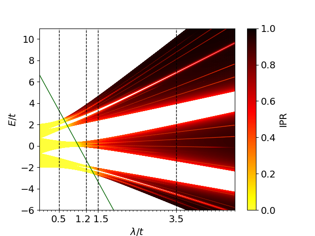
Figure 1: The spectrum and inverse participation ratio (IPR) of the noninteracting generalized Aubry-André model at $\alpha=0.3$ with various $\lambda$ and any $t>0$, obtained by diagonalizing single-particle Hamiltonians. For the length, we use a Fibonacci number ${N=F_{16}=987}$, which allows us to use periodic boundary conditions and minimize boundary effects with the frequency ${b=F_{15}/F_{16}}$ approximating the inverse golden ratio. The distinction between delocalized ($\text{IPR}\sim 1/N$) and localized ($\text{IPR}>1/N$, increasing to 1) behavior on either side of the self-dual line $\alpha E=2(t-\lambda)$ (green) is clear. Disorder strengths $\lambda$ studied herein in the interacting case are marked in black.

II The generalized Aubry-André model

II.1 The non-interacting case

The generalized Aubry-André model (GAA) [33] we consider is defined, in the non-interacting case, by the Hamiltonian

$$\begin{split}H_{0}=&\ t\sum_{n=1}^{L-1}(\psi_{n}^{\dagger}\psi_{n+1}+\psi_{n+1}^{\dagger}\psi_{n})\\ &+2\lambda\sum_{n=1}^{L}\frac{\cos(2\pi bn+\phi)}{1-\alpha\cos(2\pi bn+\phi)}\psi_{n}^{\dagger}\psi_{n},\end{split}$$ (1)

which becomes the standard Aubry-André model when $\alpha=0$, with the phase $\phi$ determining a family of “disorder realizations”. We also use the standard choice of $b$ as the inverse golden ratio $\frac{2}{1+\sqrt{5}}$. When $t>0$ and $|\alpha|<1$, this has been determined to be self-dual for energies

$$\alpha E=2(t-\lambda).$$ (2)

One may diagnose localization in this model on either side of this self-dual line, e.g. by using the inverse participation ratio (IPR), as shown in Fig. 1. For a single-particle state $|\psi\rangle$ with wavefunction $\psi_{i}$, the inverse participation ratio is defined as

$$\mathrm{IPR}=\frac{\sum\limits_{i=1}^{L}|\psi_{i}|^{4}}{\left(\sum\limits_{i=1}^{L}|\psi_{i}|^{2}\right)^{2}}.$$ (3)

When excitations are localized (to a region that does not scale with system size), $\mathrm{IPR}\sim O(1)$, whereas thermalization implies $\mathrm{IPR}\sim O(1/L)$. As predicted by self-duality, there is a mobility edge for nonzero $\alpha$ at $E=\frac{2}{\alpha}(t-\lambda)$.

II.2 The interacting model

Later works considering an interacting version of this model [38, 39, 40], constructed with the simple addition of a four-fermion term

$$H=H_{0}+V\sum_{n}\psi_{n}^{\dagger}\psi_{n}\psi_{n+1}^{\dagger}\psi_{n+1},$$ (4)

have analyzed it with exact diagonalization for small sizes and low filling factors.

The main goal of this work is to expand the system size substantially using the SIMPS method [36]. The tradeoff for large system sizes is that the finite bond dimension cuts off the entanglement of the state. If the many-body state obtained by SIMPS is localized then the entanglement does not scale with the cut size and is unaffected by the increasing bond dimension. However, a thermalized state should have volume-law entanglement scaling: in particular, the half-cut entanglement entropy should be asymptotically proportional to the system size. Since the bond dimension of an MPS is exactly the Schmidt rank across a given cut, the single-cut entanglement entropy of an MPS with (maximal) bond dimension $\chi$ is limited to precisely $\log\chi$, making the bond dimension of an adequate MPS representation exponential in the system size as a function of the cut size. Thus we trade system-size limitations suffered in exact diagonalization methods with finite-entanglement limitations due to limited bond dimension. The advantage of this tradeoff is that we can benchmark states against fully localized and fully delocalized systems in terms of how their properties scale with the bond dimension while making finite-size effects negligible.

II.3 Model parameters

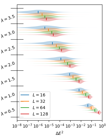
Figure 2: A violin plot displaying the distribution of energy errors at several system sizes and disorder strengths $\lambda$, given bond dimension ${\chi=10}$; tests sample the full range of the energy spectrum. One can tell that the distributions are qualitatively different among the lowest three system sizes, whereas they are qualitatively similar for $L=64$ and $L=128$. (Meanwhile, a quantitative comparison is complicated by a need to account for both extrinsic scaling of $E$ and exponential suppression of level spacing.)

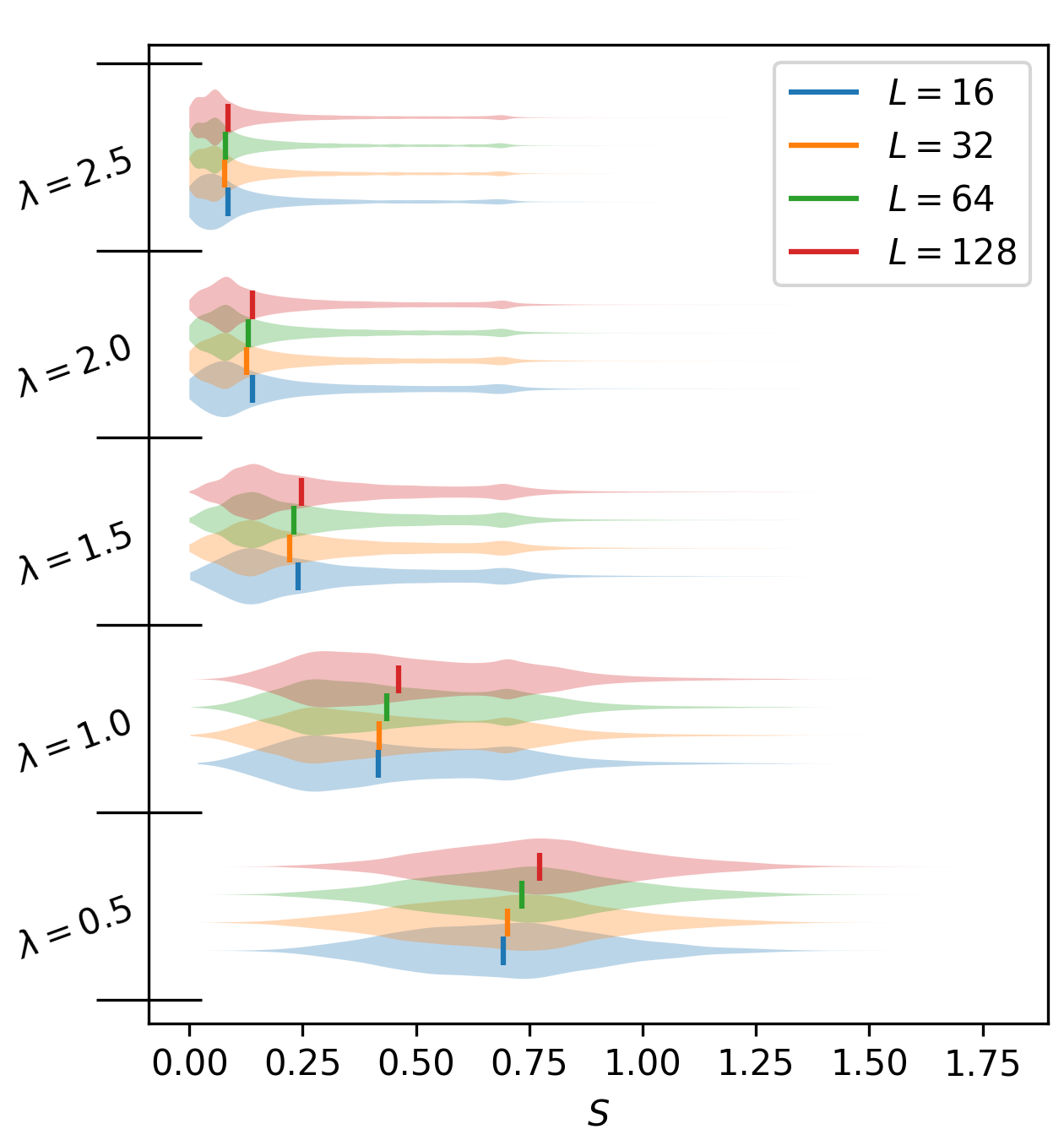
Figure 3: Entropy distribution for several values of the disorder strength $\lambda$, given various system sizes with bond dimension $\chi=10$. We find that, for a given $\lambda$, the behavior at different system sizes has few qualitative differences; we may find some for the thermalizing regime (here $\lambda=0.5$ and $\lambda=1$) between $L=16$ and $L=32$ and between $L=32$ and $L=64$, but only a modest and expected difference in the location of the median between $L=64$ and $L=128$. This helps us demonstrate that finite-size effects are minimal (particularly in comparison to finite-entanglement effects) by the time we reach $L=64$.

The systems we will be primarily considering will have an interaction strength $V/t=1$ and a mobility-edge parameter $\alpha=0.3$. We enforce particle-number conservation as a global $U(1)$ symmetry in order to restrict to half-filling. In preliminary studies we have varied the system size: with half-integer disorder strengths $\lambda=\{0.5,1,1.5,2,2.5,3,3.5\}$, six disorder realizations $\phi=\pi n/3$, and system sizes $L=\{16,32,64,128\}$, we used bond-dimension $\chi=10$ SIMPS to probe the system at equally-spaced test energies encompassing the entire spectrum. As shown in Figures 2 and 3, these studies have demonstrated to our satisfaction that finite-size effects are sufficiently small for system sizes of order $L\geq 64$. In Appendix C.2, we additionally compare data obtained from the primary studies (described below)—in particular those with smaller bond dimensions—with tests run using the same parameters but larger bond dimensions, and determine that we do not see a significant qualitative difference. Finally, we note that even the longest-lived boundary effects seen in this work, as found e.g. in Sec III.2 do not penetrate beyond a distance from the boundary of $\ell\sim 15$. Thus, for the primary studies discussed herein, we select a fixed size $L=64$.

We choose sample “disorder strengths” $\lambda$ of $0.5,1.2,1.5,3.5$. As illustrated in Fig. 1, these are, respectively, well before, intersecting, just beyond, and well beyond the single-particle mobility edge. The intention behind these choices is as follows:

• $\lambda=0.5$ should be well within the thermalizing phase and therefore should provide a benchmark for SIMPS output in this paradigm (i.e. when eigenstates are volume-law and therefore unrepresentable as MPS).

• $\lambda=3.5$ should be well within the localized phase and therefore should provide a benchmark for SIMPS output in this paradigm (when eigenstates should be easily representable with MPS).

• $\lambda=1.2$ and $\lambda=1.5$, meanwhile, provide candidates for a mobility edge, wherein results can be compared to the above benchmarks to determine whether a given energy range corresponds to the localized or thermalized phase.

Finally, we select 12 disorder realizations via phases $\phi=\pi n/6$. In each system, for each of the bond dimensions 10, 14, 20, 25, and 30, we sample 99 target energies equally spaced within each of two energy ranges, determined as follows. We can readily approximate the minimum and maximum energies $E_{\mathrm{min}}$ and $E_{\mathrm{max}}$ given half filling and fixed $t,\lambda,V,\alpha,b,\phi,$ and $L$, $E_{\mathrm{min}}$ being the ground-state energy of $H$ and $-E_{\mathrm{max}}$ being the ground-state energy of $-H$. Then the energy densities $E_{\mathrm{min}}/L$ and $E_{\mathrm{max}}/L$ will have minimal dependence on $\phi$ and $L$, so, fixing $t,V,\alpha,b$, we can define an energy density above the ground state

$$\varepsilon\equiv\frac{E-E_{\mathrm{min}}}{L}$$ (5)

which specifies $E$ for a given $L$ and $\lambda$ and which has

$$0\leq\varepsilon\leq\varepsilon_{\mathrm{max}}\equiv(E_{\mathrm{max}}-E_{\mathrm{min}})/L.$$

We use “lower” and “middle” energy ranges

• $0.1\varepsilon_{\mathrm{max}}<\varepsilon<0.15\varepsilon_{\mathrm{max}}$ (a target energy density of $\varepsilon_{m}=(0.1+0.0005m)\varepsilon_{\mathrm{max}}$ for $m=1,2,\ldots,99$)

• $0.45\varepsilon_{\mathrm{max}}<\varepsilon<0.5\varepsilon_{\mathrm{max}}$ (a target energy density of $\varepsilon_{m}=(0.4+0.0005m)\varepsilon_{\mathrm{max}}$ for $m=1,2,\ldots,99$)

Note that, for each energy range and each value used of the “disorder” strength $\lambda$ and the bond dimension $\chi$, we have a sample size of 1188 states.

III The numerical method

Friesdorf et al. [41] have shown that matrix product states can efficiently represent excited eigenstates of localized systems and are therefore an effective means of non-perturbatively analyzing localized systems at large system sizes. To extract MPS approximations of eigenstates, we use the SIMPS algorithm [36], which we outline in detail in Appendix A. SIMPS and other MPS algorithms can only attempt to diagonalize a system under the assumption that it is localized, meaning that they will otherwise give “false positives” of relatively low-entanglement states which are not approximations of any eigenstates and are instead linear combinations of states with similar entropies. Indeed, if we assume a typical energy spacing, at a typical energy $E$, of $s\sim 2^{-L}E$ (where $L$ is the system size), an equal combination of $n$ adjacent states would have energy variance on the order of $\Delta E^{2}/E^{2}\sim\frac{n^{2}}{12}2^{-2L}$ (see (6) of the Appendix). At a system size $L=64$, such a combination could still have energy error below machine precision if it consisted of $2^{33}$ distinct eigenstates. However, our intuition and the benchmarks we use suggest this is not the case, e.g., a low-energy-error superposition like that would still have comparably high entropy and thus could not be replicated as an MPS.

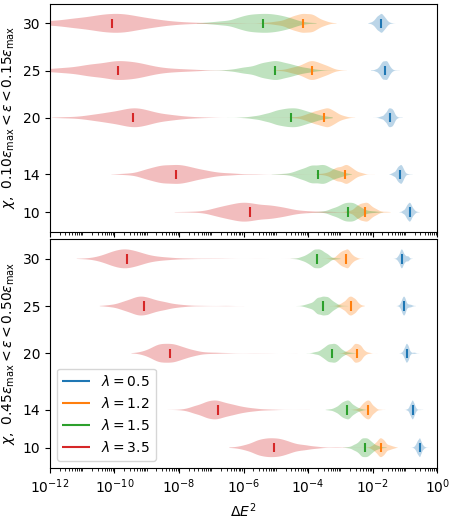
Figure 4: A violin plot representing the distribution of energy error for various disorder strengths; the area of a shape in a given region approximates the frequency of samples within the 1188 sample states, and lines are placed at the medians. In all cases, the error substantially decreases with bond dimension; however, the errors at $\lambda=0.5$ and $\lambda=3.5$ are, for all bond dimensions, at substantially different scales. The energy errors for $\lambda=1.2$ and $\lambda=1.5$, meanwhile, only approach either scale at high bond dimension, when the $\lambda=1.5$ low-energy case begins to overlap low-bond-dimension results from the localized case.

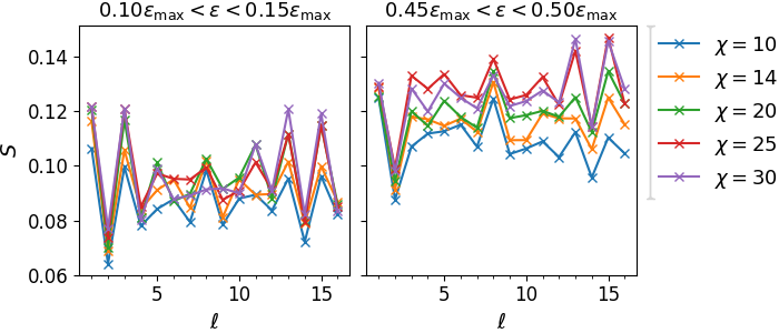
Figure 5: Single-cut entropy by cut location (i.e. distance from the nearest endpoint) for strong disorder, $\lambda=3.5$, at $L=64$. The entropy has evidently saturated by $\chi=30$ for the different cuts and energies, under consideration, and it remains low moving into the bulk, as is generally expected for the area-law behavior of localized states.

We note that, in the similar case of MPS approximations to critical ground states, there exist well-established scaling relations [42, 43]. These relations include the asymptotic behavior of the correlation length with respect to (a) the single-cut entanglement entropy, (b) the bond dimension, and (c) the energy error relative to the true ground state. Such a relation, applied to excited states of disordered ergodic systems, would be necessary in order to distinguish with any certainty the phases we hope to observe. In the absence of such an asymptotic description, we attempt to extract empirical relationships and benchmarks with respect to fully localized and fully delocalized cases which can help separate localized and ergodic phases.

III.1 Benchmark I: SIMPS applied to a fully-localized many-body system

We begin by applying SIMPS to the disorder strength $\lambda=3.5$, that is, we tune the system to be far into the region corresponding to single-particle localization. In Fig. 4, we see that the states we find given these parameters have very low energy variance $\Delta E^{2}$. In fact, for high bond dimensions $\chi>20$, $\Delta E^{2}$ appears to saturate at about $10^{-10}$, of order comparable to the tolerance of the subroutines of our SIMPS implementation. We then consider entanglement entropy, as in Fig. 5. We see, first, that as a function of bond dimension the entropy has also largely saturated by $\chi=30$ (in fact, in the entropy histograms discussed in Appendix D.2 we find the entropy distribution has largely converged with respect to bond dimensions). Indeed, the movement we see before that point is likely attributable to a reduction of bias against higher-entropy states. Moreover, we observe that neither the single-cut entropy nor the bond-dimension corrections to it grow significantly as we move into the bulk of the system, ruling out the possibility that our evidence of localization can be viewed primarily as a finite-size effect.

We also point out a distinct feature in the single-cut entropy displayed in Fig. 5, namely, the highly discrete, oscillatory behavior as the cut size $l$ varies. This feature is absent in the weak-disorder case, e.g., $\lambda=0.5$ in Fig. 6.

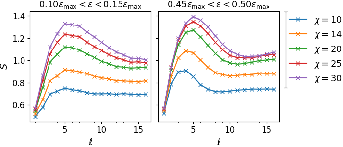
Figure 6: Single-cut entropy by cut location for weak disorder, $\lambda=0.5$, at $L=64$. While there are signs of convergence (to volume-law behavior) very close to the boundary, as seen in greater detail in Fig. 8, in general the entropy is high and failing to converge. Also notably, it peaks near the boundary, at a location $\ell\sim 5$ that grows with the bond dimension, and then falls to a bulk value, suggesting a higher-order artifact of finite-entanglement scaling beyond simply limiting the entropy.

III.2 Benchmark II: SIMPS applied to a fully delocalized system

The SIMPS algorithm naturally fails with any finite bond dimension for the fully delocalized case due to volume law entanglement scaling. Nonetheless, we can quantify this failure in the form of energy variance and entanglement scaling with bond dimension. Within our model, the “disorder” strength $\lambda=0.5$ (and other parameters as above) corresponds to full delocalization in the single-particle case. We find in Fig. 4 for the system size $L=64$ that the energy errors are very large, eclipsing the values that would be predicted by naïvely combining the cutoff error and density of states. The implication of this is promising: even as the system size becomes large, the algorithm cannot produce pseudo-eigenstates of the delocalized system which exploit tight energy spacings to exhibit small energy error.

In Fig. 6, we find rapid growth of entanglement entropy as we move up to 5 sites into the bulk of the system; notably, while a failure to converge is apparent away from the boundary, near the boundary we see convergence to something resembling a volume law. The full entanglement distribution is given in Appendix D.2. Further away from the boundary, we see the entanglement entropy fall again before settling into asymptotic behavior; this is evidently an artifact of finite entanglement given that the peak moves away from the edge as we increase the bond dimension.

We emphasize that in the weak-disorder regime studied in this section, the single-cut entropy vs. the cut size $l$ is smooth, in contrast to the previous larger disorder strength case with $\lambda=3.5$, where there were distinct, highly discrete oscillations.

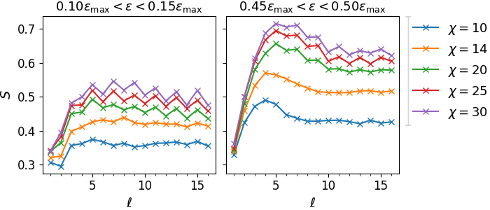
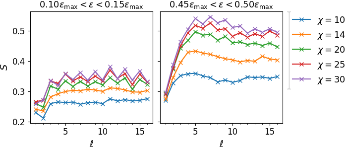
Figure 7: Single-cut entropy by cut location for disorder strengths $\lambda=1.2$ (top) and $\lambda=1.5$ (bottom) both at $L=64$. Convergence within the bulk by $\chi=30$ is apparent only in the lower energy range with $\lambda=1.5$. In the higher energy range, meanwhile, we observe for both $\lambda$ convergence towards the boundary to apparently volume-law behavior as well as a clear peak in the entropy at $\ell\sim 5$, as is also seen with $\lambda=0.5$ in Fig. 6. The substantial oscillations seen in the entropy here, including an observed fall-off between the first and second sites seen for smaller bond-dimension in the cases nearer the band edge, are discussed in more depth in Appendix B.

IV Evaluating candidate disorder strengths for a mobility edge

Now we present the main results of this paper. In the presence of the single-particle mobility edge, the localization properties of the many-body interacting states can in principle have four outcomes: (1) all many-body states are localized; (2) the many-body spectrum has a mobility edge; (3) all many-body states are delocalized; and (4) the spectrum contains spectrum containing non-ergodic extended states (the exotic case). Even though the SIMPS algorithm cannot unambiguously discriminate among all of these four scenarios, it can locate the existence of localized states in the many-body spectrum in an energy-resolved way. Thus we can address the question of whether the many-body spectrum contains any localized states when the single-particle spectrum possesses a mobility edge within numerically accessible bond dimensions.

We consider the disorder strengths $\lambda=1.2$, for which a full single-particle band is delocalized, and $\lambda=1.5$, which is fully localized (but with longer localization length in bands closer to the critical line of the mobility edge than in benchmark I, $\lambda=3.5$), as shown in Fig. 1. In Fig. 4 we have seen that the energy error in either case does not truly match either the localizing or the thermalizing case, and it is not clear from a qualitative analysis which comparison is stronger. We also see evidence in Fig. 7 that the states in middle of the spectrum, where we see convergence toward volume-law entropy scaling up to $\ell\simeq 4$, are more delocalized than those near the edge of the band, where we only see a hint of entropy scaling with cut size.

In Fig. 8, we plot entanglement entropy versus bond dimension at small cut sizes ($\ell=2,3,4,5$) averaged over the energy windows selected near the band edge and center (the full distribution of entanglement entropy for this case is explored in Appendix D.2). Within the bond dimensions we have used, we only observe saturation of entanglement entropy with bond dimension (as occurs in benchmark I) in the band-edge case of $\lambda=1.5$. In the absence of such saturation, we can still use the dependence of entanglement on both cut sizes (i.e., for single cuts, the distance between the cut and the boundary) and bond dimension.

For the case of $\lambda=1.2$, we see in Fig. 7 that the average entropy at both the band center and the band edge seem to contain features from both benchmark I (fully localized case) and II (the fully delocalized case). However, with the increasing bond dimensions it seems to develop more features of the localized state. For small bond dimensions, the entanglement curves are somewhat smooth for both energy ranges we have probed. But as the bond dimension increases, the converged curves begin to exhibit highly discrete oscillation, similar to the regime of large disorder strength. Such oscillation in the entanglement entropy was observed previously in the ground state of the XXZ spin chain [37] for open boundary conditions, and identified as a dimerization process universal in ground states of models with a Luttinger liquid description. We suspect that the presence of oscillations due to open boundary conditions may indicate the beginning of the convergence of the SIMPS algorithm toward capturing a faithful MPS representation. Note that the success of SIMPS at a finite bond dimension itself is evidence of the non-thermal nature of the state. On the contrary, for a thermal or a fully delocalized state, one would expect these oscillations to develop only at bond dimensions of the order $\chi\sim 2^{L/2}$.

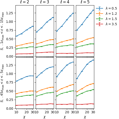
Figure 8: Average single-cut entanglement entropy, together with the standard error of the mean, as a function of the bond dimension $\chi$ for several small cuts in the various cases considered. We expect to see logarithmic growth with eventual convergence either to a constant value (in the localized, area-law case) or a value proportional to the distance from the boundary (in the delocalized, volume-law case). The asymptotic behavior generally anticipated in the bulk is logarithmic growth if the entropy is volume-law and convergence if it is area-law; near the boundary, in the volume-law case, we expect convergence to a value determined by that volume law.

V Conclusions

We have observed what appears to be a compelling distinction between thermalized and localized behavior in an interacting quasiperiodic system at a reasonably large system size $L=64$. In particular, we find that we can extract “good” eigenstates with low entropy when the strength of the quasiperiodic “disorder” is high; conversely, when it is low, we only find eigenstates of poor quality (as measured by the energy error) whose entanglement entropy moreover increases substantially with bond dimension in accordance with a volume law. When we compare these two cases with intermediate cases selected for the possibility of seeing a mobility edge, we find at the disorder strength $\lambda=1.5$ evidence broadly consistent with the claim that localization is present for lower energies but not for energies towards the middle of the spectrum. The case for delocalization is weaker at $\lambda=1.5$, but in both cases we cannot make conclusive inferences from the data taken.

In addition to studying the same systems at larger bond dimension, we could seek precise criteria for distinguishing states close to and far from true eigenstates. In the absence of such a criterion, we are unable to say for certain when the apparent saturation of entropy actually corresponds to having found true localized states. It would be further useful to establish a rigorous theoretical relationship between the bond dimension and entropy for MPS approximating extended excited states akin to the finite-entanglement scaling relationship found for critical systems in [42]. We leave this effort for future work.

It may also be worthwhile in future work to modify the numerical techniques in order to study bond-dimension scaling. For example, it may be useful to take a candidate eigenstate from a lower bond dimension as an initial state (rather than a random state) in order to see how robust that state is. It may similarly be useful to track failure of convergence instead of simply designating a maximum number of iterations and not distinguishing between “convergence” from the two stopping criteria. Meanwhile, it may improve efficiency to allow bond dimension to vary within a system (so that one may effectively save resources on “weak” bonds).

Note added: After our initial submission of this work, there have been subsequent developments that indicate that well-studied localization transitions do not exist at the expected parameters: [13, 14, 15, 16, 17] in particular, in the random-field Heisenberg model, a standard workhorse for studying MBL, the critical disorder strength once expected to be around $W=3$ may instead be as high as $W_{c}\sim 20$ [15, 16]. Our results do not directly address these questions. It is more focused instead on developing systematic matrix product methods to investigate aspects of localization transitions and, in particular, the possible existence of a many-body mobility edge in the GAA model.

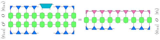
Figure 9: The tensor equation underlying the SIMPS algorithm developed in Yu, Pekker, & Clark[36] : for $O=H-E_{0}$, update $|\psi_{i+1}\rangle$ by solving for the light-blue tensor $T$ (and then decompose $T$ using SVD). The purpose of this is to optimize $\langle\psi_{i+1}|O^{\dagger}|\psi_{i}\rangle$ subject to the constraint $\langle\psi_{i+1}|O^{\dagger}O|\psi_{i+1}\rangle=1$, but with a Lagrange multiplier, absorbed into $T$, that can be solved for with normalization.

Appendix A The SIMPS algorithm

In order to perform the SIMPS algorithm, as with other DMRG-based MPS algorithm, we begin by expressing the Hamiltonian as an automaton-style matrix product operator, formed in this case from the Jordan-Wigner transform of the fermionic Hamiltonian, expressed in terms of operator-valued matrices as

$$O_{n} =\left(\begin{array}[]{ccccc}\mathbbm{1}&0&0&0&0\\ \sigma_{-}&0&0&0&0\\ \sigma_{+}&0&0&0&0\\ \frac{\sqrt{V}}{2}\sigma_{z}&0&0&0&0\\ \frac{W_{n}}{2}\sigma_{z}-E_{0}\mathbbm{1}&\sigma_{z}\sigma_{+}&\sigma_{-}\sigma_{z}&\frac{\sqrt{V}}{2}\sigma_{z}&\mathbbm{1}\\ \end{array}\right),$$

$$W_{n} =2\lambda\frac{\cos(2\pi bn+\psi)}{1-\alpha\cos(2\pi bn+\phi)},$$

with boundary vectors $v_{L}=(0,0,0,0,1)$ and $v_{R}=(1,0,0,0,0)$.

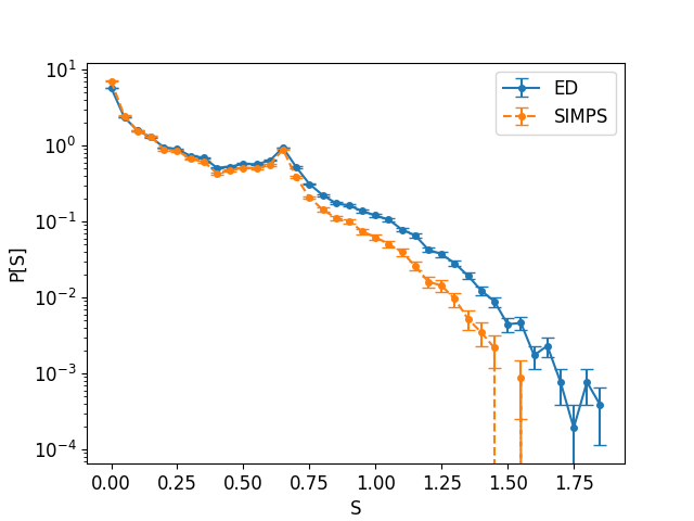
Figure 10: A replication of the test run by Yu, Pekker, and Clark to eliminate entropy bias of the SIMPS algorithm from consideration. The disordered Heisenberg model, with disorder strength $W=8$, is analyzed for 101 disorder realizations on a 10-site spin chain. Each of the $2^{L}$ eigenstates are extracted via exact diagonalization; then SIMPS, with bond dimension $\chi=12$, is used for $2^{L}$ equally-spaced target energies, with post-processing to remove duplicates (if $|\langle\psi_{i}|\psi_{j}\rangle|>0.3$, we exclude the state with greater $\Delta E^{2}$). This produces 103,424 states via exact diagonalization and 45,917 states via SIMPS. The latter is about three times as many states as in the original test, which explains the difference in noise in that case. As with the original visualization, SIMPS yields significantly fewer states at nearly all entropy ranges, the exceptions being the particularly small ones ($S\leq 0.2$) and the “resonance” peak at $S=\log 2$, with the difference in frequency being visibly greater at, e.g., $S\sim 1$ compared to $S\sim 0.5$.

To find an eigenstate,

1. Start with an initial matrix-product ansatz $|\psi_{0}\rangle$ and a target energy $E_{0}$, incorporated into the MPO as above.

2. Given an iteration $|\psi_{i}\rangle$, optimize the next iteration $|\psi_{i+1}\rangle$ as follows:

3. $|\psi_{i+1}\rangle$ may be initialized randomly, but we have, following a suggestion by Clark[44], initialized it with $|\psi_{i}\rangle$

4. Site-by-site, optimize $|\psi_{i+1}\rangle$ to satisfy $(H-E_{0})|\psi_{i+1}\rangle=\psi_{i}$: that is, apply the shifted and inverted Hamiltonian.

5. To do so, we represent this equation as the maximization of $\langle\psi_{i+1}|(H-E_{0})|\psi_{i}\rangle$, subject to the constraint $\langle\psi_{i+1}|(H-E_{0})^{2}|\psi_{i+1}\rangle=\|\psi_{i}\|^{2}$ which will be uniquely satisfied by $(H-E_{0})^{-1}\psi_{i}$.

6. This is done, site-by-site, by solving the diagrammatic equation in Fig. 9 for individual tensors. We note that we find it preferable to update two sites at once (i.e. the tensor being optimized consists of the contraction of tensors at two sites), especially when enforcing charge/fermion-number conservation, in order to speed up convergence. The resulting two-site tensor is then split via SVD to update the MPS.

7. This may be repeated until $|\psi_{i+1}\rangle$ has converged; alternatively, when initializing $\psi_{i+1}$ with $\psi_{i}$, very few sweeps (optimizing the tensors at each site) may be conducted per iteration, as the goal of convergence is the eigenvalue equation $\psi\propto(H-E_{0})\psi$, which should be more accurate after each sweep.

8. Repeat until the energy has converged, or until a maximum number of iterations has been reached.

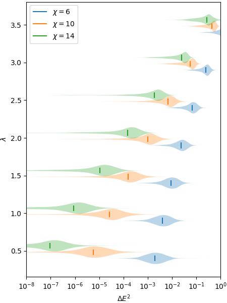
Figure 11: The distribution of energy errors at several (smaller) bond dimensions, given system size $L=128$, for tests sampling the full spectra of systems with $\lambda\in\{0.5,1.0,1.5,2.0,2.5,3.0,3.5\}$

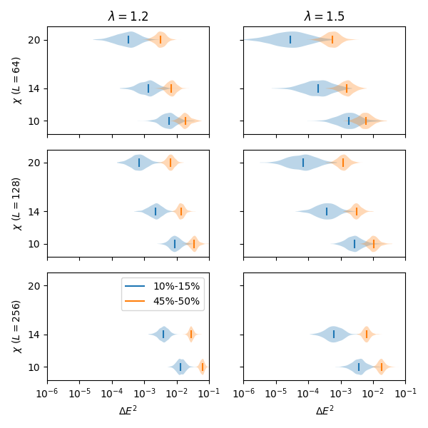
Figure 12: A violin plot displaying the distribution of energy errors, in the systems under consideration within the main text but for a greater selection of system sizes: for $\chi\in\{10,14,20\}$, the systems are analyzed at $L=128$, and for $\chi\in\{10,14\}$, the systems are analyzed at $L=256$. Note that the the $L=64$ data is contained within Fig. 4 of the main text. This plot demonstrates that, with these parameters, system size does not affect the quality of states within the sizes considered.

In the original work of Yu, Pekker, and Clark [36], the authors claim that SIMPS is “sampling states at a given entanglement with the same frequency as ED and hence there is no systemic bias.” This would be quite remarkable, given the general expectation that entropy may diverge approaching a transition - in particular, for any bond dimension $\chi$ there should be truly localized states with entanglement entropy at some cut in excess of the maximum $\log\chi$. (In fact, in a good approximation of a physical state, it may be expected that the entropy ceiling should be even less than that absolute maximum, as, for example, was shown for infinite MPS approximations for ground states of critical spin chains by Pollmann et al. [42].) Although they acknowledge a “failure of SIMPS to find high-quality eigenstates in [the] near-ergodic and ergodic regime”, they do not explain why there should be a hard boundary between regimes near to and far from ergodicity. Moreover, in the data they provide as evidence for this claim (Fig. S2), the divergence of the proportion of SIMPS states from that of ED states at higher entanglement entropy seems apparent (if small), and likely statistically significant. To confirm statistical significance, we replicate the test they use to produce these data as faithfully as possible, yielding data that clearly replicates the major features of this figure, particularly a divergence between sampling rates at higher entropies, in Fig. 10.

In addition to favoring true low-entropy eigenstates, we have noted that the SIMPS algorithm will produce “false” eigenstates when no low-entropy eigenstates are available, as is evidenced by the fact that the algorithm produces any states at all within the presumed ergodic regime. To attempt to constrain the false eigenstates we observe, we may try to approximate a worst-case scenario by supposing that there exist $n$ consecutive eigenstates, of some separation $s$: that is, taking the crudest possible approximation, the energies take the form $E_{k}=E_{0}+ks$. Then the energy variance would be

$$\begin{split}\Delta E^{2}&\equiv\langle H^{2}\rangle-\langle H\rangle^{2}=\langle(H-E_{0})^{2}\rangle-\langle H-E_{0}\rangle^{2}\\ &=\sum_{k=0}^{n-1}\frac{s^{2}k^{2}}{n}-\left(\sum_{k=0}^{n-1}\frac{sk}{n}\right)^{2}=\frac{n(n-1)}{12}s^{2}.\end{split}$$ (6)

We do not presuppose the order of magnitude of $n$, as the possible entropy reduction from such a combination is highly dependent on the nature of the eigenstates themselves. We may, however, presume that the worst-case energy spacing $s$ is of the order $2^{-L}$, such that

$$\Delta E^{2}\sim\frac{n^{2}}{12}\frac{L^{2}}{2^{2L}}.$$ (7)

For the system sizes under consideration this is well below machine precision; it will likely be necessary to include further assumptions, e.g. from the random matrix theory formulation of ETH, in order to find a reasonable lower bound.

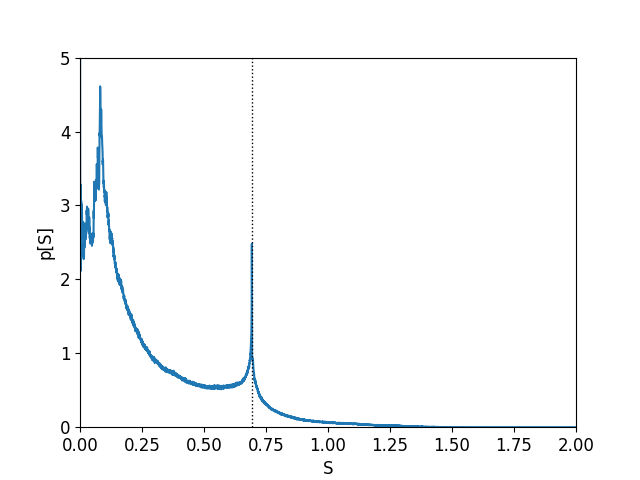
Figure 13: A histogram of all single-cut entropies, for all states, of 12-site systems with $\lambda=2$, given 1920 “disorder realizations” (i.e. phases $\phi$). This demonstrates a very clear resonance peak at $S=\ln 2$, marked by the dotted line.

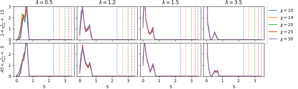
(a) $\ell=1$

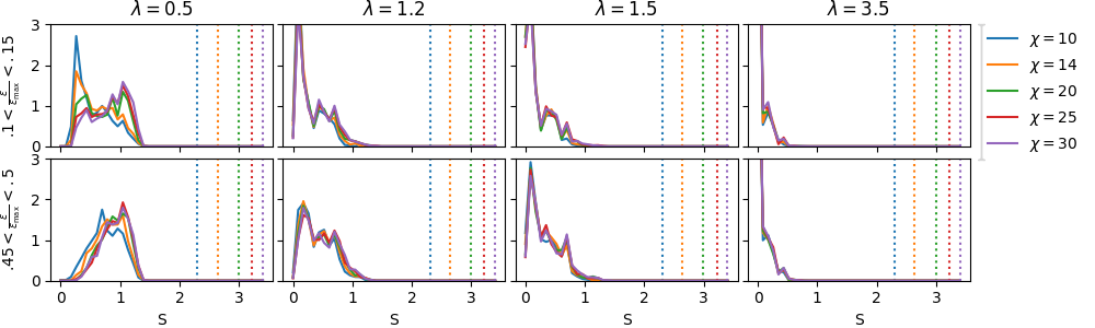
(b) $\ell=2$

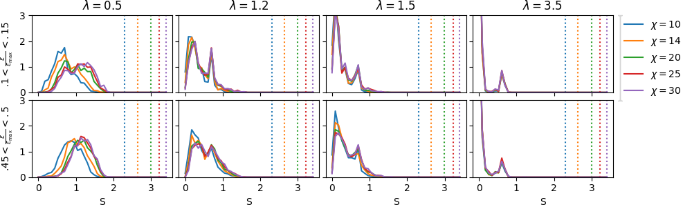
(c) $\ell=3$

(d) $\ell=4$

(e) $\ell=5$

Figure 14: Histograms of single-cut entanglement entropy by cut position, corresponding to the data in Fig. 8 of the main text

(a) $\ell=6$

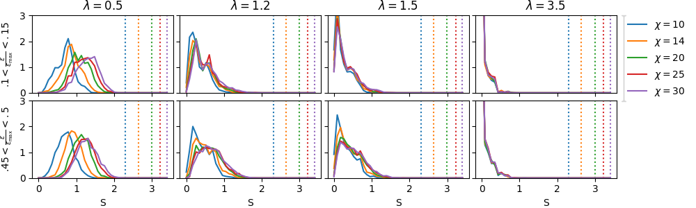
(b) $\ell=7$

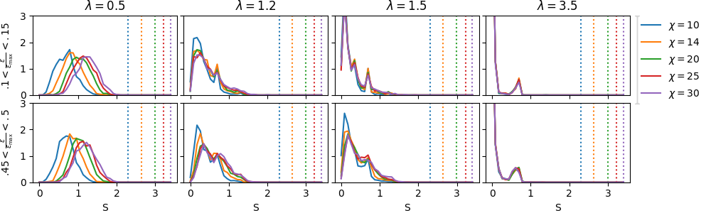
(c) $\ell=8$

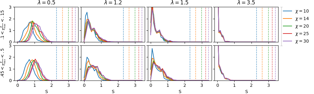
(d) $\ell=9$

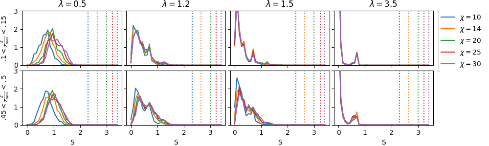
(e) half-cut

Figure 15: Histograms of single-cut entanglement entropy by cut position, corresponding to the data in Fig. 17 of the main text, as well as (e) histograms of half-cut entanglement entropy (i.e. $\ell=32$ for $L=64$)

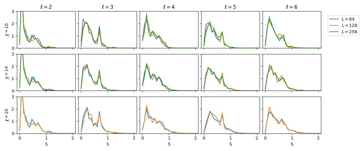
(a) $\lambda=1.2$, lower energy range

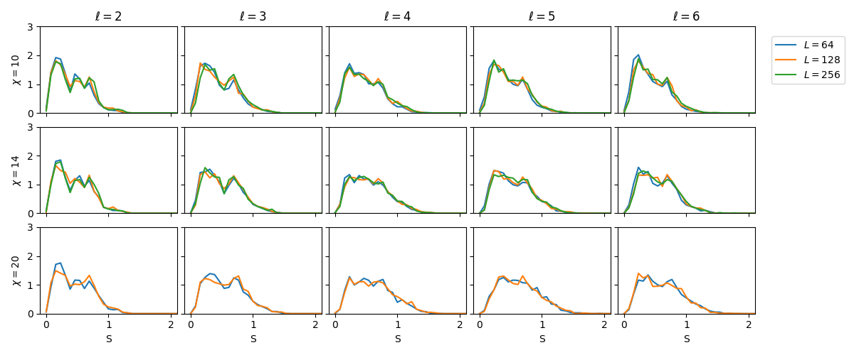
(b) $\lambda=1.2$, higher energy range

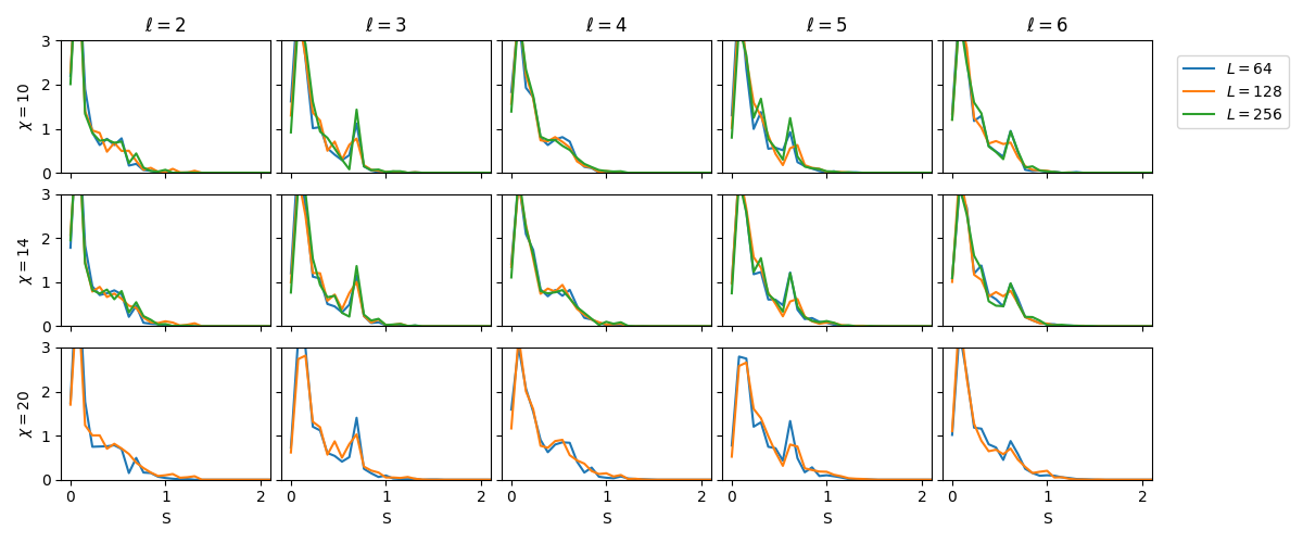
(c) $\lambda=1.5$, lower energy range

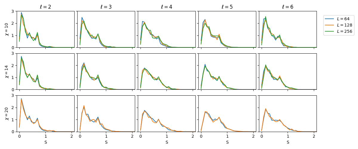
(d) $\lambda=1.5$, higher energy range

Figure 16: Histograms of single-cut entanglement entropy in different regimes, plotted for different cut locations (from $\ell=2$ to $\ell=6$) and bond dimensions and compared across lengths.

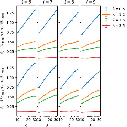
Figure 17: Average single-cut entanglement entropy, together with the standard error of the mean, as a function of the bond dimension $\chi$ for several larger cuts (as in Fig. 8 of the main text but with the subsequent four cuts).

Appendix B Entropy oscillations

A characteristic effect seen in the localized regime (and even at higher bond dimensions) is the oscillation of single-cut entanglement entropy as a function of cut location; this effect is most clearly seen in Fig. 5 but is also visible in Fig. 7 at higher bond dimensions. The more detailed histograms in Figures 14 and 15 show peaks in the entanglement entropy which seem less prominent across even-numbered cuts and in more thermalized conditions. We confirm in Fig. 13 that these peaks are not spurious by analyzing a collection of systems at size $L=12$ with exact diagonalization; this additionally lets us conclude with high confidence that the typical location of the peaks is at $S=\ln 2$. We may understand these entropy peaks as indicating the presence of a dimer: taking a pair of qubits in the “single-occupancy” subspace $\operatorname{span}\{|01\rangle,|10\rangle\}$, uniformly distributed over the Bloch sphere, define a random variable $\mathrm{S}_{\text{dimer}}$ to be the entanglement entropy between them. Then the various histograms under consideration are, for the most part, qualitatively consistent with drawing the entropy from $\mathrm{S}_{1}+\mathrm{S}_{\text{dimer}}$ with probability $p_{\text{dimer}}$ and $\mathrm{S}_{0}$ with probability $1-p_{\text{dimer}}$, given a pair of well-behaved, unimodal random variables $\mathrm{S}_{0}$ and $\mathrm{S}_{1}$.

It is worth noting as well that such entropy oscillations are often seen in models of spinless fermion chains with tight-binding couplings or (equivalently, under the Jordan-Wigner transformation) Heisenberg-like antiferromagnetic spin chains when open boundary conditions break translation symmetry [45, 37, 46]. In particular, Laflorencie et al. [37] have identified this effect as a dimerization process universal in ground states of models with a Luttinger liquid description (such as the critical XXZ chain), determining that the alternating parts of the energy and entropy, $E_{A}$ and $S_{A}$ respectively, should have proportional universal contributions which may be expressed as

$$S_{A}(\ell,L)\propto E_{A}(\ell,L)\sim\left[\frac{L}{\pi}\sin\left(\tfrac{\pi\ell}{L}\right)\right]^{-K}$$

for the $\ell$th cut of a length-$L$ chain in a system with Luttinger parameter $K$.

Appendix C Additional datasets

In addition to the dataset described and referenced in the main text, we have two additional datasets that we will reference on occasion in these Supplemental Materials. As in the main text, each uses the Hamiltonian defined by (1) and (4), with $\alpha=0.3$, $t=V=1$, and $b=\frac{2}{1+\sqrt{5}}$, and with protection of $U(1)$ symmetry to restrict to half-filling.

C.1 Exploratory trials

We began by testing a wide range of disorder strengths across the spectrum. For disorder strengths $\lambda$ in 0.5, 1.0, 1.5, 2.0, 2.5, 3.0, and 3.5 (that is, the half-integers between 0 and 4), we took 24 disorder realizations (that is, values of $\phi$ in (1)). With bond dimension $\chi=10$, we analyzed systems of size $L=16,32,64,128$; we additionally applied bond dimensions $\chi=6$ and $\chi=14$ to systems of size $L=128$. In each case, we selected 400 target energies that encompass the full energy spectrum (noting that this means we would see, and reject, a number of copies of the states with lowest and highest energy). We have used this dataset to produce Figures 2, 11, and 3. In the latter, we also have a subset of those conditions, namely $\chi=10$ and $\chi=14$ for $L=128$, with $\lambda=1.2$.

C.2 Comparison of system sizes

By examining the system at smaller length scales, we have been able to conclude that at least the most dramatic finite-size effects do not persist into the system size where the main trials were conducted. We have additionally taken the parameters for the “intermediate regime” under primary consideration, $\lambda=1.2$ and $\lambda=1.5$ with energy density $0.1\varepsilon_{\text{max}}<\varepsilon<0.15\varepsilon_{\text{max}}$ and $0.45\varepsilon_{\text{max}}<\varepsilon<0.5\varepsilon_{\text{max}}$, and extracted candidate eigenstates as in the main trials with the larger system sizes $L=128$ (for $\chi=10,\ 14,\ \&\ 20$) and $L=256$ (for $\chi=10\ \&\ 20$). In Fig. 12, we examine the energy error from these trials and find that it does not vary substantially when we increase system size. We have also been able to use the single-cut entanglement entropy to observe the boundary effects, seeing in Figures 6 and 7 that even the most persistent boundary effects do not appear to persist far enough into the bulk to make a significant difference in the cases being considered. In Fig. 16 we take a closer look by comparing entropy histograms at various cuts across system sizes, finding that there is little consistent variation as we increase system size (and that what variation there is, is not monotonic, as the $L=256$ graphs tend to seem closer to the $L=64$ graphs than to the $L=128$ ones.)

Appendix D Review of diagnostic metrics

In the main text we have relied primarily on two metrics, energy error and single-cut entanglement entropy, to evaluate the goodness and behavior of candidate eigenstates. Here we review these metrics, including more detailed plots summarizing entanglement-entropy distributions, and then discuss several additional metrics not utilized in the main text.

D.1 Energy error

We have presented our primary results on the energy error in Fig. 4; we show additional results for larger system sizes in Fig. 12. We here note briefly how it is calculated. In particular, it emerges fairly easily from SIMPS calculation: contracting the transfer matrices used to obtain the LHS of Fig. 9 gives $\langle(H-E_{0})^{2}\rangle$, and $\langle H-E_{0}\rangle$ (which does not come pre-calculated) is easily computed through the simpler contraction of the RHS of the same (replacing $|\psi_{i}\rangle$ with $|\psi_{i+1}\rangle$.)

In Figs. 2 and 11, we introduce an additional set of simulations, in which we sampled the entire spectrum for a substantial number of “disorder” strengths $\lambda$, with bond dimensions among $\{6,10,14\}$ and lengths (for $\chi=10$; otherwise $L=128$) in $\{16,32,64,128\}$, to examine how our results scale with bond dimension and with system size.

D.2 Single-cut entanglement entropy

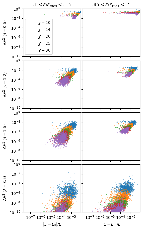
Figure 18: Scatter plot of energy error versus energy wandering, to attempt to determine whether a relation exists between quality of states & how far from the target energy the algorithm must “wander” to find it

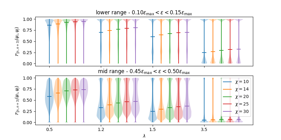
(a) width 3

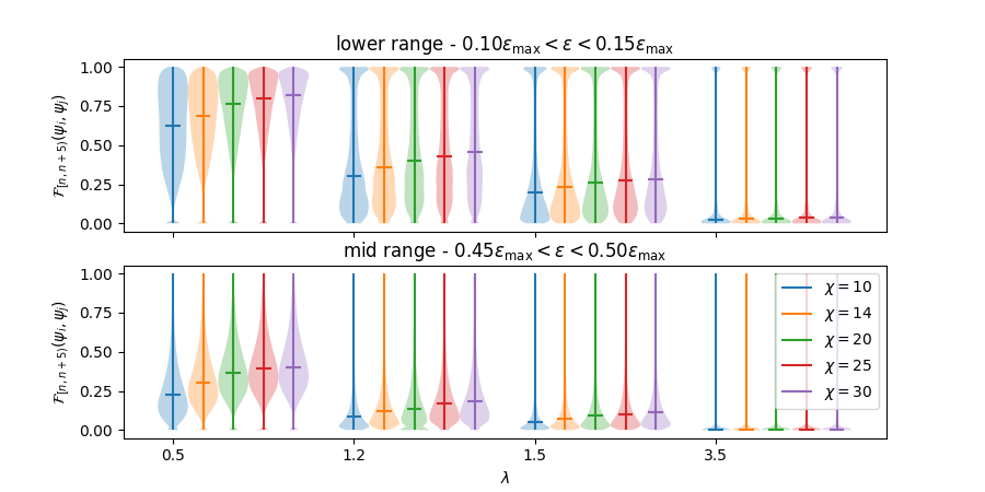
(b) width 5

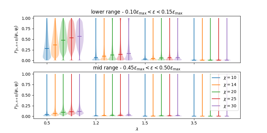
(c) width 8

Figure 19: Violin plots of Uhlmann fidelities among systems with various disorder strengths and at different energy ranges, for segments of width (a) 3, (b) 5, and (c) 8. All fidelities calculated are between states with the same disorder strength and disorder sample, bond dimension, and energy range. All segments of the given length within the 64-site chain are considered.

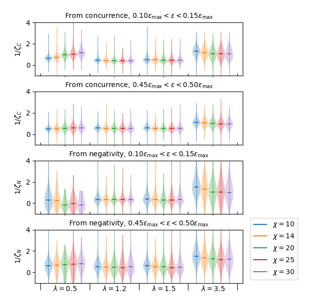
Figure 20: Violin plots of (inverse) localization lengths among systems with various disorder strengths and at different energy ranges, taking a weighted average of the (inverse) lengths for each state analyzed

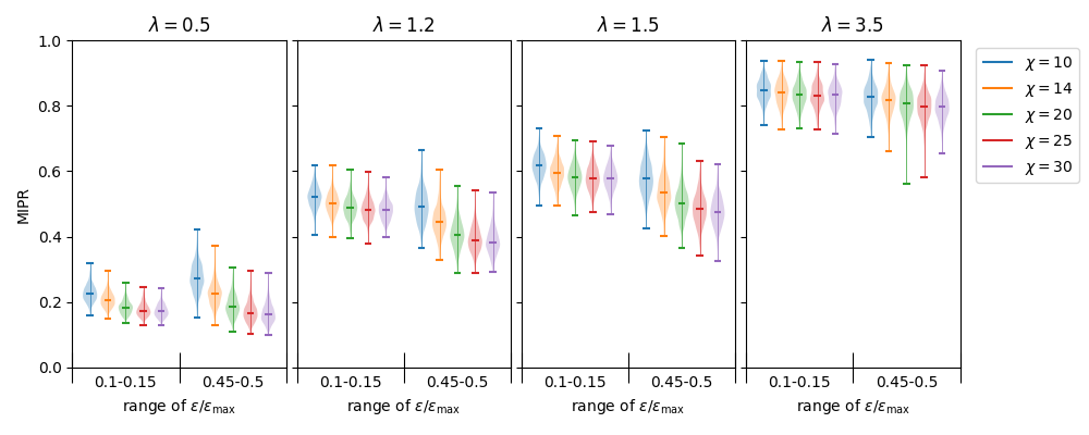
Figure 21: Violin plots of the many-body inverse participation ratio for states in the main datasets

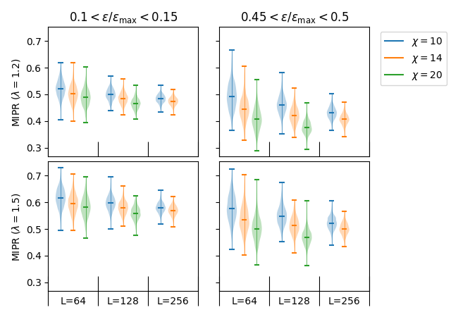
Figure 22: Violin plots comparing many-body inverse participation ratio across system sizes

By keeping the MPS in (bi)canonical form, we are able to extract entanglement entropies directly from the Schmidt coefficients which are stored as part of the ansatz. We have explored how average entropies, at given distances from the boundary, scale with the bond dimension $\chi$ in Figs. 8, 5, 6, and 7 of the main text. In particular, in Fig. 8, we examined the entropy scaling at several specific cuts; we repeat this further into the bulk in Fig. 17, and then go deeper by examining the corresponding entropy distributions in each case in Figures 14 and 15, respectively. Similar entropy distributions are examined in Fig. 16, there comparing entropy histograms at different system sizes to investigate whether boundary effects show system-size dependence at the primary length $L=64$ considered. In Fig. 3, we take a different approach and examine the entropy distribution for all cuts at various $\lambda$, $L$, and $\chi$. One feature that is clearly visible in many of these histograms is a peak at $S=\ln 2$, corresponding to dimers or two-site resonances. We confirm that this is not a numerical artifact using exact diagonalization in Fig. 13.

D.3 Energy wandering

Another quantity we may use to diagnose the goodness of states is the so-called “energy wandering”, the difference between the energy of a state and the target energy used to obtain it. The idea behind using this is to determine whether or not approximate eigenstates of adequate quality are sufficiently common. In Fig. 18 we compare the distribution of values of $\|E-E_{0}\|$ with that of $\Delta E^{2}$.

D.4 Uhlmann fidelities

Inspired by, and using methods based on, [47], we compute Uhlmann fidelities: if the reduced density matrix of an eigenstate $\psi_{i}$ on a segment $A$ is $\rho_{i,A}=\operatorname{tr}_{A}|\psi_{i}\rangle\langle\psi_{i}|$, then the Uhlmann fidelity between $\psi_{i}$ and $\psi_{j}$ on $A$ is

$$\mathcal{F}=\operatorname{tr}\sqrt{\sqrt{\rho_{i,A}}\rho_{j,A}\sqrt{\rho_{i,A}}}.$$ (8)

Ideally,

• In the localized case, the distribution of these quantities will be determined by so-called “l-bits”: if $\psi_{i}$ and $\psi_{j}$ differ on an l-bit whose support is within $A$, then $\mathcal{F}=0$; if they agree on all l-bits mostly supported within $A$, then $\mathcal{F}\sim 1$; and intermediate values will only occur when there are l-bits on which $\psi_{i}$ and $\psi_{j}$ differ that have significant support both inside and outside of $A$.

• In the fully ergodic regime, where $\rho_{i,A}$ should be fully determined by the energy (as $\operatorname{tr}_{A}\exp(-\beta(E_{i})H)$, with $\beta(E_{i})$ the inverse-temperature corresponding to $E_{i}$), we expect a less discrete distribution of $\mathcal{F}$, with values continuously dependent on the energy difference and stochastically dependent on the choice of region $A$.

In Fig. 19, we examine the distribution of Uhlmann fidelities in various systems considered, for various sizes of region $A$. We see that the typical behavior, in the localized case, is a bimodal distribution with one narrow peak at 0 corresponding to cases differing on l-bits supported in $A$ and another narrow peak at 1 corresponding to cases agreeing on l-bits overlapping $A$, with the former shrinking and the latter growing both as the size of $A$ increases (so that $\mathcal{F}=1$ would require agreement on more l-bits) and as we move to the higher-energy band, which we expect to have larger localization length. In the delocalized case, meanwhile, we see a broad unimodal distribution whose peak, in addition to lowering as the size of $A$ and the energy of the band increase, raises as the bond dimension increases, suggesting an increase in similarity as the accuracy improves. (It is not truly unimodal however; a small peak at $\mathcal{F}=0$ which narrows with increasing bond dimension suggests that the pseudo-eigenstates obtained in this case do sometimes have features which resemble l-bits.

In analyzing the $\lambda=1.2$ and $\lambda=1.5$ cases, we find that

• For the most part, the distribution in the higher-energy band is closer to a unimodal distribution like the one seen in the delocalized case; in (a) a second peak close to $\mathcal{F}=1$ in the width-3 distribution exists but grows less distinct with increasing bond dimension

• The distribution in the lower-energy band is more consistently bimodal, although with lower maxima at nonzero fidelity.

• In particular, as bond dimension increases the distributions in the higher-energy band appear to converge towards a unimodal distribution; this seems to be the case, though it is less clear, for the lower-energy band when $\lambda=1.2$. However, for the lower-energy band with $\lambda=1.5$, we see apparent convergence toward a bimodal distribution in (a) and (b).

D.5 Localization lengths

We follow [48, 49] in using two measures of entanglement between two qubits, negativity and concurrence, to attempt to estimate the localization length, which should diverge approaching a localization transition or mobility edge. In particular, given concurrence values $C_{i,j}$ or negativity values $N_{i,j}$ between two sites of a given state, we fit the nontrivial values to (see eqs. 21 and 22 of [49])

$$\begin{split}C_{i,i\pm n}&=k^{C\pm}_{i}\exp(-n/\zeta^{C\pm}_{i})\\ N_{i,i\pm n}&=k^{N\pm}_{i}\exp(-n/\zeta^{N\pm}_{i}).\end{split}$$ (9)

In Fig. 20, we take, for each state, an average of all these $1/\zeta^{C\pm}_{i}$ and, separately, $1/\zeta^{N\pm}_{i}$, weighted by $\frac{1}{\sigma_{1/\zeta}}$. While this confirms some basic expectations – the localization lengths of eigenstates with $\lambda=3.5$ tend to be much smaller, and for both types of entanglement the lengths are greater in the middle band than in the lower band – at other times the results are unexpected or even self-contradictory, for example, when the typical localization length appears to decrease with bond dimension and when it is lower for $\lambda=1.2$ and $\lambda=1.5$ than for $\lambda=0.5$. We must therefore conclude that we will not be able to perform much meaningful analysis on this data.

D.6 Inverse participation ratio

In analysis performed following the initial submission of this work, we apply the many-body generalization of the inverse participation ratio (3), which has been defined [50, 51], for a system with $N$ fermionic orbitals of which $N_{f}=\nu N$ are occupied,

$$\mathcal{I}=\frac{1}{1-\nu}\left(\frac{1}{N_{f}}\sum_{i}\langle\hat{n}_{i}\rangle^{2}-\nu\right)$$ (10)

where $\hat{n}_{i}$ is the number operator for the $i$th orbital. This ensures that this many-body inverse participation ratio (MIPR), $\mathcal{I}$, interpolates between $\mathcal{I}=0$ in the ideal thermalized case where all sites have equal filling, $\langle\hat{n}_{i}\rangle=\nu$, and $\mathcal{I}=1$ in the ideal localized case when filling is deterministic, $\langle\hat{n}_{i}\rangle=1$ with probability $\nu$ and $\langle\hat{n}_{i}\rangle=0$ with probability $1-\nu$.

Here each site hosts one orbital, $N=L$, and half-filling or $\nu=1/2$ makes

$$\mathcal{I}=-1+\frac{4}{L}\sum_{i}\langle\hat{n}_{i}\rangle^{2}.$$

In Fig. 21 we examine the distribution of the MIPR in states obtained for the main dataset. In the localized benchmark ($\lambda=3.5$) we find that the MIPR is large and does not vary substantially with bond dimension, whereas in the thermalized benchmark ($\lambda=0.5$) we find the MIPR to be small and consistently decreasing with bond dimension. For the mobility-edge candidate regime, we find an intermediate MIPR that is roughly constant with bond dimension for the lower-energy regime and decreasing with bond dimension for the higher-energy regime, suggesting that both $\lambda=1.2$ and $\lambda=1.5$ remain compatible with a many-body mobility edge.

In Fig. 22 we use the MIPR to compare the main dataset with states obtained in larger systems (i.e. those analyzed in Fig. 12), finding that the distributions tighten but otherwise remain qualitatively similar.

References

- Deutsch [1991] J. M. Deutsch, Physical review a 43, 2046 (1991).
- Srednicki [1994] M. Srednicki, Physical review e 50, 888 (1994).
- Basko et al. [2006] D. M. Basko, I. L. Aleiner, and B. L. Altshuler, Annals of physics 321, 1126 (2006).
- Imbrie [2016a] J. Z. Imbrie, Journal of Statistical Physics 163, 998 (2016a).
- Imbrie [2016b] J. Z. Imbrie, Physical review letters 117, 027201 (2016b).
- Schreiber et al. [2015] M. Schreiber, S. S. Hodgman, P. Bordia, H. P. Lüschen, M. H. Fischer, R. Vosk, E. Altman, U. Schneider, and I. Bloch, Science 349, 842 (2015).
- Bordia et al. [2016] P. Bordia, H. P. Lüschen, S. S. Hodgman, M. Schreiber, I. Bloch, and U. Schneider, Physical review letters 116, 140401 (2016).
- Chiaro et al. [2019] B. Chiaro, C. Neill, A. Bohrdt, M. Filippone, F. Arute, K. Arya, R. Babbush, D. Bacon, J. Bardin, R. Barends, et al., arXiv preprint arXiv:1910.06024 (2019).
- Weiner et al. [2019] F. Weiner, F. Evers, and S. Bera, Phys. Rev. B 100, 104204 (2019).
- Suntajs et al. [2020] J. Suntajs, J. Bonca, T. Prosen, and L. Vidmar, Phys. Rev. E 102, 062144 (2020).
- Schulz et al. [2020] M. Schulz, S. R. Taylor, A. Scardicchio, and M. Znidaric, Journal of Statistical Mechanics: Theory and Experiment 2020, 023107 (2020).
- Taylor and Scardicchio [2020] S. R. Taylor and A. Scardicchio, arXiv preprint arXiv:2007.13783 (2020).
- Abanin et al. [2021] D. Abanin, J. H. Bardarson, G. De Tomasi, S. Gopalakrishnan, V. Khemani, S. Parameswaran, F. Pollmann, A. Potter, M. Serbyn, and R. Vasseur, Annals of Physics 427, 168415 (2021).
- Sels and Polkovnikov [2021] D. Sels and A. Polkovnikov, Physical Review E 104, 054105 (2021).
- Sels [2021] D. Sels, arXiv preprint arXiv:2108.10796 (2021).
- Morningstar et al. [2022] A. Morningstar, L. Colmenarez, V. Khemani, D. J. Luitz, and D. A. Huse, Physical Review B 105, 174205 (2022).
- Sierant and Zakrzewski [2022] P. Sierant and J. Zakrzewski, Physical Review B 105, 224203 (2022).
- Turner et al. [2018] C. Turner, A. Michailidis, D. Abanin, M. Serbyn, and Z. Papić, Physical Review B 98, 155134 (2018).
- Kjäll et al. [2014] J. A. Kjäll, J. H. Bardarson, and F. Pollmann, Physical review letters 113, 107204 (2014).
- Li et al. [2015] X. Li, S. Ganeshan, J. Pixley, and S. D. Sarma, Physical review letters 115, 186601 (2015).
- Modak and Mukerjee [2015] R. Modak and S. Mukerjee, Physical review letters 115, 230401 (2015).
- Serbyn et al. [2015] M. Serbyn, Z. Papić, and D. A. Abanin, Physical Review X 5, 041047 (2015).
- Luitz et al. [2015] D. J. Luitz, N. Laflorencie, and F. Alet, Physical Review B 91, 081103 (2015).
- Geraedts et al. [2017] S. D. Geraedts, R. N. Bhatt, and R. Nandkishore, Physical Review B 95, 064204 (2017).
- Goihl et al. [2019] M. Goihl, J. Eisert, and C. Krumnow, Physical Review B 99, 195145 (2019).
- Yao and Zakrzewski [2020] R. Yao and J. Zakrzewski, arXiv preprint arXiv:2002.00381 (2020).
- Brighi et al. [2020] P. Brighi, D. A. Abanin, and M. Serbyn, Physical Review B 102, 060202 (2020).
- Chanda et al. [2020] T. Chanda, P. Sierant, and J. Zakrzewski, Phys. Rev. Research 2, 032045 (2020).
- De Roeck et al. [2016] W. De Roeck, F. Huveneers, M. Müller, and M. Schiulaz, Phys. Rev. B 93, 014203 (2016).
- Lüschen et al. [2018] H. P. Lüschen, S. Scherg, T. Kohlert, M. Schreiber, P. Bordia, X. Li, S. D. Sarma, and I. Bloch, Physical review letters 120, 160404 (2018).
- Kohlert et al. [2019] T. Kohlert, S. Scherg, X. Li, H. P. Lüschen, S. D. Sarma, I. Bloch, and M. Aidelsburger, Physical Review Letters 122, 170403 (2019).
- Guo et al. [2021] Q. Guo, C. Cheng, Z.-H. Sun, Z. Song, H. Li, Z. Wang, W. Ren, H. Dong, D. Zheng, Y.-R. Zhang, et al., Nature Physics 17, 234 (2021).
- Ganeshan et al. [2015] S. Ganeshan, J. H. Pixley, and S. Das Sarma, Phys. Rev. Lett. 114, 146601 (2015), arXiv:1411.7375 [cond-mat.dis-nn] .
- Hsu et al. [2018] Y.-T. Hsu, X. Li, D.-L. Deng, and S. D. Sarma, Physical Review Letters 121, 245701 (2018).
- An et al. [2020] F. A. An, K. Padavić, E. J. Meier, S. Hegde, S. Ganeshan, J. Pixley, S. Vishveshwara, and B. Gadway, arXiv preprint arXiv:2007.01393 (2020).
- Yu et al. [2017] X. Yu, D. Pekker, and B. K. Clark, Phys. Rev. Lett. 118, 017201 (2017).
- Laflorencie et al. [2006] N. Laflorencie, E. S. Sørensen, M.-S. Chang, and I. Affleck, Physical review letters 96, 100603 (2006).
- Li et al. [2015] X. Li, S. Ganeshan, J. H. Pixley, and S. Das Sarma, Phys. Rev. Lett. 115, 186601 (2015), arXiv:1504.00016 [cond-mat.str-el] .
- Li et al. [2016] X. Li, J. H. Pixley, D.-L. Deng, S. Ganeshan, and S. Das Sarma, Phys. Rev. B 93, 184204 (2016), arXiv:1602.01849 [cond-mat.stat-mech] .
- Deng et al. [2017] D.-L. Deng, S. Ganeshan, X. Li, R. Modak, S. Mukerjee, and J. H. Pixley, Annalen der Physik 529, 1600399 (2017), arXiv:1612.00976 [cond-mat.str-el] .
- Friesdorf et al. [2015] M. Friesdorf, A. H. Werner, W. Brown, V. B. Scholz, and J. Eisert, Phys. Rev. Lett. 114, 170505 (2015).
- Pollmann et al. [2009] F. Pollmann, S. Mukerjee, A. M. Turner, and J. E. Moore, Phys. Rev. Lett. 102, 255701 (2009), arXiv:0812.2903 [cond-mat.str-el] .
- Stojevic et al. [2015] V. Stojevic, J. Haegeman, I. P. McCulloch, L. Tagliacozzo, and F. Verstraete, Phys. Rev. B 91, 035120 (2015), arXiv:1401.7654 [quant-ph] .
- [44] B. Clark, personal communication.
- Affleck et al. [2009] I. Affleck, N. Laflorencie, and E. S. Sørensen, Journal of Physics A: Mathematical and Theoretical 42, 504009 (2009).
- Wang [2004] X. Wang, Phys. Rev. E 69, 066118 (2004).
- Hauru and Vidal [2018] M. Hauru and G. Vidal, Phys. Rev. A 98, 042316 (2018).
- Bera and Lakshminarayan [2016] S. Bera and A. Lakshminarayan, Phys. Rev. B 93, 134204 (2016).
- West and Wei [2018] C. G. West and T.-C. Wei, arXiv e-prints , arXiv:1809.04689 (2018), arXiv:1809.04689 [quant-ph] .
- Bera et al. [2015] S. Bera, H. Schomerus, F. Heidrich-Meisner, and J. H. Bardarson, Phys. Rev. Lett. 115, 046603 (2015).
- Vu et al. [2022] D. Vu, K. Huang, X. Li, and S. Das Sarma, Phys. Rev. Lett. 128, 146601 (2022).