Bayesian semiparametric modelling of covariance matrices for multivariate longitudinal data
Abstract
The article develops marginal models for multivariate longitudinal responses. Overall, the model
consists of five regression submodels, one for the mean and four for the covariance matrix, with the latter
resulting by considering various matrix decompositions.
The decompositions that we employ are intuitive, easy to understand, and they do not rely on any assumptions
such as the presence of an ordering among the multivariate responses. The regression submodels
are semiparametric, with unknown functions represented by basis function expansions. We use spike-slap
priors for the regression coefficients to achieve variable selection and function regularization,
and to obtain parameter estimates that account for model uncertainty.
An efficient Markov chain Monte Carlo algorithm for posterior sampling is developed.
The simulation studies presented investigate the effects of priors on posteriors, the gains that one may have when
considering multivariate longitudinal analyses instead of univariate ones, and whether these gains
can counteract the negative effects of missing data.
We apply the methods on a highly unbalanced longitudinal dataset with four responses observed over of period of years.
Keywords: Cholesky decomposition; Clustering; Model averaging; Semiparametric regression; Variable selection; Variance-correlation separation
1 Introduction
There is a variety of systems that evolve over time and are too intricate to be appropriately characterized by a single outcome variable. Consider for example ‘cognition’, the topic of the data example presented later in this article. According to the American Psychological Association’s Dictionary of Psychology, cognition is a term that refers to ‘all forms of knowing and awareness, such as perceiving, conceiving, remembering, reasoning, judging, imagining, and problem solving’. Cognition is a complex, not directly observable, system that evolves over time. Measuring cognitive function relies on administering multiple psychometric tests, and investigating how it evolves and declines in the elderly requires observations over multiple years. Analysing datasets generated by such investigations requires flexible regression models for multivariate longitudinal responses. The main goal of this article is to develop, within a Bayesian framework, marginal models for multivariate longitudinal continuous responses, non-parametrically linking the mean vectors and covariance matrices to the covariates. The current literature on modelling covariance matrices for multivariate longitudinal data relies on decompositions of the covariance matrices that are either difficult to interpret or that make assumptions that are not tenable. Here, we avoid all such decompositions and we only utilize those that are easy to understand and justify.
In order to set the notation, let denote a vector of responses observed at time point , , the -dimensional vector of all responses, and the covariance matrix of . Matrix must satisfy the positive definiteness (pd) condition, and that creates a major challenge when modelling its elements as functions of covariates. To ensure that this condition is satisfied, it is necessary to factorized into a product of matrices. The decomposition (Hamilton,, 1994)
| (1) |
has been utilized for modelling multivariate longitudinal data by Xu & Mackenzie, (2012), Kim & Zimmerman, (2012), Kohli et al., (2016) and Lee et al., (2020). Matrices and have the following structures
| (11) |
where submatrices are unconstrained, while submatrices are pd, , and all submatrices in and are of dimension . The following interpretation that has appeared in, among others, Pourahmadi, (1999) and Daniels & Pourahmadi, (2002) for the univariate case, and Xu & Mackenzie, (2012) and Kim & Zimmerman, (2012) for the multivariate case, provides justification for the lack of constraints on the elements of and the pd constraint on the elements of . For the sake of simplicity we assume that vectors have zero mean. Let denote the linear least squares predictor of based on its predecessors and let denote the prediction error. It can be shown that the predictor is expressed in terms of the negatives of the submatrices of as
| (12) |
Further, the prediction error variance is given by the corresponding block of i.e. . To see how factorization (1) is satisfied, let . We have that , and since consecutive prediction errors are uncorrelated, it follows that . The sets of matrices and have been termed the generalized autoregressive matrices and innovation covariance matrices of (Xu & Mackenzie,, 2012).
A simple modification of (1) can provide an alternative interpretation. Since has the same block triangular structure as , the decomposition
| (13) |
also holds, where has the same structure as . This decomposition, for univariate responses, has been studied by Zhang & Leng, (2012), and for multivariate ones by Feng et al., (2016). With this decomposition, the submatrices of that are below the main diagonal can be interpreted as moving average coefficient matrices in a time series context, hence, again, they are unconstrained.
In this article, we adopt the decomposition in (1) that leads to the interpretation in (12). Since matrices are unconstrained, their elements can be modelled utilizing semiparametric regression models. These are described in Section 2.
The decompositions in (1) and (13) have been unanimous among researchers modelling multivariate longitudinal data. By contrast, there have been several proposals for modelling the innovation covariance matrices . These are reviewed in the next paragraph. The difficulty in modelling these matrices arises from having to satisfy the pd condition and from the absence of any natural ordering in the elements of the errors .
Based on the spectral decomposition and the matrix logarithmic transformation (Chiu et al.,, 1996), Xu & Mackenzie, (2012) model matrices in terms of the explanatory variable ‘time’, . Further, based on the modified Cholesky decomposition (Pourahmadi,, 1999, 2000), i.e. the decomposition in (1) applied for , Kim & Zimmerman, (2012) model the innovation covariance matrices as functions of . Lastly, Kohli et al., (2016) avoid decompositions and instead model each using linear covariance models (Anderson,, 1973), that is, , where are known pd matrices and are unknown weights, . The spectral decomposition and the modified Cholesky decomposition outside the context of longitudinal studies, lack simple statistical interpretation. Further, the linear covariance model does not express the matrices in terms of covariates and its implementation in practice can be difficult. For instance, the best performing model in the study of Kohli et al., (2016) does not guarantee that the estimated covariance matrix is pd.
A decomposition, however, that is statistically simple and intuitive, was proposed by Barnard et al., (2000). It separates the matrices into diagonal matrices of innovation variances and innovation correlation matrices , . With this decomposition it is easy to model the innovation variances in terms of covariates as the only constrained they must satisfy is the positiveness. This was the approach taken by Lee et al., (2020) and the approach that we take in this article too.
As was remarked by Pourahmadi, (2007), of the available decompositions, the separation of variances and correlations is the least effective in satisfying the pd condition. Clearly, this condition must now be satisfied by the innovation correlation matrices . To overcome this condition, and model the elements of a single correlation matrix in terms of covariates, Zhang et al., (2015) utilize the Cholesky decomposition , parametrizing the non-zero elements of using hyperspherical coordinates. In the applications presented by Zhang et al., (2015), the elements of are modelled in terms of covariate ‘lag’. Lee et al., (2020) follow the same approach as Zhang et al., (2015), but merely reparametrise the innovation correlation matrices without modelling their elements in terms of covariates. In the data analysis they presented, this resulted in a common, time invariant, innovation correlation matrix, even though they stressed the importance of correctly specifying the correlation structure.
Here, we take a different, more intuitive approach, by specifying a normal prior on the Fisher’s transformation of the nonredundant elements of the matrices ,
| (14) |
where denotes the space of correlation matrices and the indicator function that maintains positive definiteness. In addition, the indicator function truncates the range of the correlations and induces dependence among them (Daniels & Kass,, 1999). Due to this truncation, parameters and are no longer interpreted as the mean and variance of the distribution. Here, we model both parameters as unknown functions of time , and .
The model in (14) can be restrictive because it only allows for a single function that is common to all correlations. However, it is conceivable that correlations evolve differently over time. Failing to specify a prior that allows for the needed flexibility can have a negative impact on the estimated correlations, especially in small samples (Daniels & Kass,, 1999). Here, this flexibility is reached by considering mixtures of normal distributions . We refer to this model as the ‘grouped correlations model’ (Liechty et al.,, 2004). We also consider a ‘grouped variables model’ that clusters the variables instead of the correlations and it is more structured than the grouped correlations model.
The overall model consists of regression submodels. These are the models for the mean of the response vector, the elements of the generalized autoregressive matrices, the innovation variances, and the parameters of distribution of the innovation correlation matrices. In the approach presented here, each regression model involves nonparametrically modelled effects, represented utilizing basis function expansions. We enable flexible estimation by utilizing several basis functions and we implement variable selection and function regularization by utilizing spike-slab priors (see e.g. George & McCulloch, (1997)). The work presented in this article builds upon the work of Chan et al., (2006) and Papageorgiou, (2018) who describe methods for univariate response regression with nonparametric models for the mean and variance, and the work of Papageorgiou & Marshall, (2020) who presented methods for multivariate response regression with nonparametric models for the means, the variances and the correlation matrix.
We develop an efficient stochastic search variable selection algorithm by using Zellner’s g-prior (Zellner,, 1986) that allows integrating out the regression coefficients in both the mean function of the responses and the parameter (or ) of the innovation correlation matrices. In addition, the Markov chain Monte Carlo (MCMC) algorithm generates the variable selection indicators in blocks (Chan et al.,, 2006; Papageorgiou,, 2018) and selects the MCMC tuning parameters adaptively (Roberts & Rosenthal,, 2001).
The remainder of this article is arranged as follows. Section 2 describes the model in detail and Section 3 describes the main elements of the MCMC algorithm. All the details of the MCMC algorithm are available in the supplementary material. In Section 4 we present results from simulation studies. The first one investigates how posteriors, based on different priors, concentrate around the true covariance and correlation matrices, while the second one investigates the gains that one may have, in terms of reduced posterior mean squared error (MSE), when fitting multivariate longitudinal models instead of univariate ones. Additionally, in the second study we examine the effects that missing data have on the posterior MSE and whether adding more than one response to the model can counteract these effects. Section 5 applies the methods on a highly unbalanced dataset on cognitive function and depressive symptomatology, with responses observed over of period of years. Section 6 concludes the paper with a brief discussion. All the methods described in this article are freely available in the R package BNSP (Papageorgiou,, 2020).
2 Multivariate longitudinal response model
Let denote the vector of responses observed on individual at time point , . Here, we allow the observational time points to be unequally spaced. We let denote the ordered set of all unique observational times, , and we denote its cardinality by . Further, let denote the covariate vector that is observed along with and that may include time, other time-dependent covariates and time-independent ones. In addition, let denote the th response vector. With and , the overall model takes the form
In the following subsections we detail how the means and covariance matrices are modelled semiparametrically in terms of covariates.
2.1 Mean model
The means are modelled utilizing semiparametric regression methods
| (15) |
where are regressors with parametrically modelled effects, are regressors with effects that are modelled as unknown functions, and denotes the total number of effects that enter the mean models.
Unknown functions are represented utilizing basis function expansions
| (16) |
where is fixed and it represents the maximum number of basis functions that can be used in modelling . Further, is the vector of basis functions and is the vector of the corresponding coefficients. Here, the basis functions of choice are the radial basis functions, given by , where are fixed knots.
The implied model for the mean of vector is
where , , and . In the final expression, and are as and but with and replaced by and .
Recalling that denotes the th response vector, we may write the mean model as , where . Alternatively, the model can be written in the usual form where and .
We note that is a maximal vector covariates and it is common to the responses. By introducing binary indicators for variable selection, we allow each response to have its own set of covariates. Vector has the same length and structure are vector , introduced just below (17), and its elements are binary indicators that select which regressors enter the mean model of the th response. Given , model (17) is written as
where consists of all non-zero elements of and of the corresponding elements of .
Letting denote the vector of binary indicators and the vector of non-zero regression coefficients for the responses, we can write the regression model for the mean of as . Similarly, we can write .
2.2 Covariance model
Let denote the covariance matrix of . As was discussed in the introduction, to model the elements of in terms of covariates, we beging by considering the factorization , where matrices and have the form shown in (11). The next two subsections describe semiparametric models for the generalized autoregressive matrices and the innovation covariance matrices .
2.3 Generalized autoregressive matrices
For , the element of , , we consider the following semiparametric model
| (18) |
where the developments in (18) follow along the same lines as those for the mean model, detailed in (15) - (17). Functions are linearised utilizing a fixed number of basis functions, . Vector denotes the maximal set covariates that is common to the autoregressive coefficients. Further, vector consists of the regression coefficients, grouped by the effect they model. Vector is the corresponding vector of binary indicators that selects which coefficients enter the model of the autoregressive coefficient. We note that here the intercepts are subject to selection. Given , model (18) is expressed as
| (19) |
where consists of all non-zero elements of and of the corresponding elements of .
Let be the vector of all regression coefficients, and be the vector of all binary indicators. Further, let be the vector of all non-zero coefficients. Now, from (12) and the definition of the prediction error, we have
| (20) |
that represents a dynamic linear model, since the design matrix involves the predecessors of . Note that, by using as subscript in a matrix , we mean the matrix with the columns that correspond to the zero elements of removed. When the mean of is not zero, we replace in (20) by its centred version . This leads to
| (21) |
which can be written in the more familiar form of a multivariate mixed model
| (22) |
where the design matrix depends on .
2.4 Innovation covariance matrices
For modelling the innovation covariance matrices , we begin by employing the separation strategy of Barnard et al., (2000), by which is decomposed into a diagonal matrix of variances and a correlation matrix ,
| (23) |
The next subsections consider models for the diagonal elements of and the correlation matrix .
2.4.1 Diagonal innovation variance matrices
It is easy to model matrix in terms of covariates as the only requirement on its diagonal elements is that they are nonnegative. It is clear that the following semiparametric model satisfies this requirement
| (24) |
Similar models for innovation variances have appeared in Leng et al., (2010) and Lin & Pan, (2013).
Consider now vectors of indicator variables for selecting the elements of that enter the th variance regression model. In line with the indicator variables for the mean and autoregressive models, these are denoted by . Given , model (24) can be expressed as
or equivalently
| (25) |
2.4.2 Time-varying innovation correlation matrices
The approach we take for modelling the correlation matrices , extends the work of Liechty et al., (2004) and Papageorgiou & Marshall, (2020) who proposed models for correlation matrices in the context of cross-sectional studies. In the context of longitudinal studies, we propose to model these matrices utilizing time as the only covariate. Hence, we use symbols to denote these matrices. Below we describe three priors, termed ‘common correlations’, ‘grouped correlations’ and ‘grouped variables’ priors.
2.4.3 Common correlations
The common correlations model is defined as follows
| (26) |
where denotes the space of correlation matrices, is the indicator function that ensures that the correlation matrix is pd and is the normalizing constant
A typical choice for is the Fisher’s transformation that leads to .
We model the parameters of this distribution using nonparametric regression, with time as the only independent variable
| (27) | |||
| (28) |
Equivalently, we can write (28) as
If the indicator function were not present in (26), then the model described in (26) - (28) could be thought of as a semi-parametric regression model for the mean and the variance of normally distributed responses (see e.g. Chan et al., (2006) and Papageorgiou, (2018)). Let vector consist of the non-redundant elements of , and let . Subject to the pd constraint, we can express the common correlations model as
| (29) |
where , is a design matrix with rows equal to and is a diagonal matrix with elements equal to , where and appear in the corresponding matrices times, the number of unique elements of .
Introducing now vectors of indicators and for selecting the elements of and that enter the models for and , respectively, model (29) can be written as
| (30) |
where and consist of the non-zero elements of and , and consists of the columns of that correspond to the non-zero elements of .
2.4.4 Grouped correlations
The common correlations model is restrictive as it implies that all correlations evolve in the same way over time. It is important, however, from a theoretical standpoint to estimate the correlation structure correctly. Hence, here we generalize the model to include multiple surfaces by considering the following prior
| (31) |
where denotes the number of surfaces in the model, is the surface assignment indicator and
In the above, are surface specific regression coefficients and are surface specific variable selection indicators, .
Let vector consist of the non-redundant elements of , assigned to surface . Further, let . Subject to the pd constraint, we can express model (2.4.4) as
| (32) |
where .
2.4.5 Grouped variables
Here we describe another clustering model that, instead of correlations, clusters the variables. We have the following prior
where
and is the number of groups in which the variables are distributed, creating clusters for the correlations.
2.5 Prior specification
In this section we specify the priors for the model parameters. We begin by describing the priors of the parameters of the mean model. For we specify a g-prior (Zellner,, 1986),
| (33) |
where , and is the covariance matrix of the , that is . Further, the prior for is taken to be an inverse Gamma, .
Consider now the vectors of variable selection indicators for the mean functions. We specify independent binomial priors for each of their subvectors,
| (34) |
where, for parametric effects, and , , while for nonparametric effects, and was defined in (16), Independent Beta priors are specified for , .
Moving on to the priors of the parameter of the autoregressive coefficients, a normal prior is specified for the non-zero coefficients of the model in (19)
For the scale parameter , we consider inverse Gamma and half-normal priors, and . Further, the specification of the priors for the vectors of variable selection indicators follows the same pattern as for indicators. That is, independent binomial priors are specified for each of the subvectors of ,
where and for and and was defined after (18) for Independent Beta priors are specified for
Next, we describe the priors for the innovation variance parameters. First, for we specify independent normal priors
Further, we consider inverse Gamma and half-normal priors for , and For the scale parameter in (25), we also consider inverse Gamma and half-normal priors, and . Continuing with the priors for the vectors of indicators , we specify independent binomial priors for each of their subvectors,
where and are analogous to and (and and ). We specify independent Beta priors for
Lastly, we describe the priors placed on the parameters of the models of the innovation correlation matrices. Starting with the ‘common correlations model’ in (30), let . The prior for the non-zero part of is the following g-prior
| (35) |
Further, the prior for is specified as Furthermore, we specify a binomial prior for vector
where denotes the number of basis functions used in linearising in (27), and . A Beta prior is specified for .
Further, the prior for is specified as
For we consider inverse Gamma and half-normal priors, and Continuing with the prior for vector , this is taken to be
where denotes the number of basis functions used in linearising in (28) and . We specify a Beta prior for . Further, we specify inverse Gamma and half-normal priors for , and
Next we describe the priors for the cluster specific parameters and prior weights of the grouped correlations model. Firstly, conditionally on , the non-zero elements of are specified to have the following prior
| if the cluster is non-empty, | |||||
| (36) |
Secondly, for vectors we specify binomial priors
with the prior on being
Lastly, the prior weights are constructed utilizing the so called stick-breaking process (Ferguson,, 1973; Sethuraman,, 1994). Let be independent draws from a distribution. We have: , for , , and . We take the concentration parameter to be unknown and we assign to it a gamma prior with mean .
In the numerical illustrations that we present in this article, we use the following priors. For we specify as a -variate analogue to the prior of Liang et al., (2008). For and we specify Beta priors. The priors on and are specified to be IG. Further, for , , and we define HN priors. Furthermore, for we specify , again, as an analogue to the prior of Liang et al., (2008). Lastly, the prior on the DP concentration parameter is specified as .
3 Posterior Sampling
Posterior sampling is carried out by expressing the likelihood function in different ways and using the expression that is more computationally convenient for each step of the MCMC algorithm. Further, where possible, we integrate out parameters to improve mixing, and where beneficial, we augment the model with additional parameters to make sampling easier. Here we only present the main concepts and a detailed description of all MCMC steps is available in the supplementary material.
We first consider the likelihood that is obtained from the normality assumption, . Due to the factorization in (1), the quadratic form of the likelihood may be written as
| (37) |
where .
Further, recalling (21) and the definition of prediction error, and the separation of variances and correlations in (23), may be written as
| (38) |
where . In the first equality, matrix is subscripted by because here we model its elements in terms of covariate ‘time’ only. In the second equality, denotes the set of unique observational time points and the set of sampling units observed at time point . We denote the cardinality of by .
In addition, recalling (20) and its centred versions in (21) and (22), we can write (37) as
| (39) |
where . We take to be a matrix of zeros when .
To improve mixing of the MCMC algorithm, we can integrate out vector from the likelihood of
| (40) |
where
, , and is the total number of columns in .
To write function in a computationally convenient way, first note that , which, due to (1), may be written as . Further, due to the separation of variances and correlations in (23), we may further express the latter as = , where . Furthermore, we write the last expression as . Likewise, we may write that . In addition, . It follows that
The most computationally expensive step of the MCMC algorithm is the one that samples from the posterior of the parameters of the correlation matrices. This is because acceptance probabilities of the Metropolis-Hastings step involve the ratio of the normalizing constants of the density in (26) (or the ones in (2.4.4) and (2.4.5)). Calculating this ratio is very computationally demanding, but it can be avoided by introducing the ‘shadow prior’ (Liechty et al.,, 2004). The basic idea is to introduce latent variables between the correlations and the means . This modifies prior (26) as follows
| (41) |
where
and is a fixed, small constant. Further, variables are independently distributed with time specific means and variances, . Hence, the semiparametric model (30) now applies on the unconstrained ,
| (42) |
Sampling from the posterior of still involves the ratio of the normalising constants of the density in (41), but that, as was argued by Liechty et al., (2004), for small , can reasonably be approximated by one.
Considering now the ‘grouped correlations’ model, with the introduction of the shadow prior, model (2.4.4) becomes the same as the one in (41). The difference is that here variables are independent with conditional distribution . Further, letting be analogous to , defined above (32), it is easy to see that semiparametric model (32) now applies on the unconstrained
| (43) |
Additionally, letting , model (43) may be written in vectorized form in precisely the same way as (42).
To improve mixing of the MCMC algorithm over the parameters of the models of the correlation matrices, we can integrate out vector from the likelihood of . The marginal of , computed from (42) and (35), is
| (44) |
where , and .
Lastly, under the grouped correlations model, the marginal likelihood of is given by
where , and .
4 Simulation Studies
We present results from two simulation studies. The first one examines how posteriors, based on different priors, concentrate around the true covariance and correlation matrices, while the second one investigates the gains that one may have, in terms of reduced posterior mean squared error (MSE), when fitting multivariate longitudinal models instead of univariate ones. Additionally, in the second study we examine the effects that missing data have on the posterior MSE and whether adding more than one response to the model can counteract these effects.
4.1 Effects of priors on the posteriors of matrices
We consider a trivariate system of responses, observed over equally spaced time points, . The single covariate here is taken to be time, . For the sake of simplicity we take the means of the three responses to be constant (zero), but we consider complex function for all other model parameters. For the autoregressive coefficients we consider
| (45) |
Further, for the diagonal innovation variance matrices we consider
| (46) |
Lastly, the innovation correlation matrices are taken to be
| (47) |
where are set equal to for the time points, respectively. The innovation correlation matrices consist of two clusters of correlations, one including elements and and the other including element . The cluster that includes two elements has parameter that changes rapidly during the first time points and slowly during the last , while the other cluster has constant zero parameter. These matrices can also be thought of as consisting of two clusters of variables, one includes variables and and the other includes variable . Generally, with clusters of variables, at most parameters are needed: to describe the correlations within the clusters and to describe the correlations between the clusters. However, because here there is a singleton cluster, we need parameters: the parameter that describes the correlation between variables and (set to ), and the parameter that describes the correlation between the clusters (set to ).
Figures 1, 2 and 3 show the true and fitted curves for the parameters described above, displayed along with credible intervals. We note that fitted curves and credible intervals were obtained based on a simulated dataset of size .
 |
 |
 |
 |
 |
 |
 |
 |
 |
 |
 |
 |
 |
Given the specifications of the autoregressive coefficients in (4.1), we construct the matrices and from them, the lower triangular matrix in (11). Further, from the specifications in (4.1) and (47), we construct the innovation covariance matrices in (23) and from them, the block diagonal matrix in (11). The covariance matrix is obtained as . We note that subscript is redundant here as the covariance matrix is common to all subjects and hence it is omitted in the sequel.
Datasets are generated from a multivariate Gaussian with mean zero and covariance . We consider sample sizes, . To obtain results that are representative and independent of the generated dataset, for each sample size we generate replicate datasets and present results that are averaged over these.
To each simulated dataset we fit models with common specifications for the mean, the autoregressive coefficients, the innovation variances, and the dispersion parameter of the correlations. The models only differ in their specification of the centre parameter of the correlations. Specifically, the means of the responses are modelled using only an intercept term, , the autoregressive coefficients are modelled using a smooth function of lag with basis functions, , where , and the basis functions where defined above (17). Further, the innovation variances are modelled using a smooth function of time, , where . Lastly, the dispersion parameter of the correlations is modelled using only an intercept term, . Concerning parameter , the first model specifies to be constant , the second one specifies to be a smooth function of time with basis functions, , while the third one specifies a grouped variables model, where the number of groups is , and each group’s mean is modelled as a smooth function of time using basis functions. We note that M3 is the correctly specified model while the other are misspecified.
For all models we run the MCMC algorithm for iterations, discarding the first as burn in, and of the remaining keeping one in two. This results in samples of innovation correlation matrices over the time points, and covariance matrices , . To evaluate the effects of priors, we compute the average distance between and using the loss function , , where the sampled matrices are based priors , , and . We denote the average loss associated with model by . As there are correlation matrices , results are presented in terms of the average risk over these matrices . Using the same loss function, we compute the average distance between the sampled and , . Recall that is the simplest possible model with only an intercept term, while and allow for single and multiple curves to be fitted, respectively. We present results in terms of the percentage improvement of the two more complex models relative to the simplest model, and , that we refer to as the relative risks.
Results are presented in Table 1. It is suggested that, for small samples, it is important to correctly model the innovation correlation matrices when either the innovation correlations themselves or the covariances/correlations among responses at each time point are of interest. From the Table we can see that both and improve over model , for the estimation of both and . Further, the relative risk of is, with one exception, less than that of . Lastly, the substantial reduction in risk observed for , decreases as the sample sizes increases, and the relative risks get close to . The exception occurs for the estimation of the with model , for which an important gain of can be observed even for .
| n | ||||
|---|---|---|---|---|
| 10 | 36.31 | 59.94 | 40.70 | 55.07 |
| 20 | 90.52 | 87.20 | 80.18 | 83.71 |
| 50 | 92.34 | 96.67 | 82.94 | 94.46 |
| 100 | 98.73 | 99.16 | 86.88 | 96.38 |
4.2 Gains
To investigate the potential gains associated with fitting multivariate longitudinal models and the effects of missing data on posterior distributions, we consider a data-generating mechanism that consists of responses, observed over time points, . The responses are generated from a multivariate normal distribution with mean , that is, the mean of the first response is a linear function of , while the other responses have constant zero mean. Further, the covariance matrix is taken to be , where is the marginal covariance matrix of and has diagonal elements equal to and all off diagonal elements equal to . The choice of autoregressive covariance structure is a standard one. It implies that correlations between observations on at different time points decrease exponentially fast as the lag increases. The value of is not of particular interest here, and hence it is fixed to , implying that correlations get halved every time the lag increases by . The structure of indicates that is equally correlated with and at all time points. This correlation is equal to at lag and it gets halved when the lag increases by .
The chosen mean and covariance structures are fairly simple, and this suffices for the purposes of the current study. The main interest here is on the quality of the estimate of the mean function of the first response. We examine how this quality, as measured by the posterior MSE, or it’s components bias and variance, depends on the dimension of the response in the fitted model, the value of the correlation coefficient , the sample size , and the percentage of missing data. The effect of the dimension of the response is evaluated by fitting -, -, and -dimensional response models. The effect of the correlation coefficient is examined by letting take values in the set . The effect of the sample size is assessed by letting take values in the set . Lastly, the effect of missing data is investigated by allowing , and chance of missing observations, utilizing a missing completely at random mechanism.
Considering a -dimensional response model as an example, the mean functions are modelled using , . This specification is correct for the first response and wrong for the other two responses. Further, the autoregressive coefficients and innovation variances are modelled using and , where and include and knots, respectively, allowing for the possibility of non-linear effects. Lastly, we fit the common correlations model (26) with constant mean, and constant variance, . These choices for and were arrived at after experimentation with more complex models that showed the more complex models to not be necessary.
The regression coefficients are taken to be and , where the value of was so chosen to achieve a signal-to-noise ratio (SNR) equal to . The SNR is defined as , where SST the total sum of squares SST= and SSE the error sum of squares SSE=. Predictions were obtained by fitting the true data-generating model.
For all models we obtain posterior samples of which we discard the first as burn in, and of the remaining we keep one in two. Based on the retained samples, we obtain samples for the parameter of main interest, , by replacing the regression coefficients and by the corresponding sampled values, . We compare fitted models in terms of their posterior bias and variance in estimating . Using subscript to denote quantities obtained from models with fitted response dimension , the posterior bias and variance are computed as and , where is the mean of . Further, because and are computed for , results are summarised by computing sums: and . Results presented below are based on replicate datasets.
Table 2 compares model performance by reporting the ratio , that we refer to as relative bias, while Table 3 compares model performance by reporting the ratio , that we refer to as relative variance, . We can see from Table 2 that relative bias decreases as the correlation between the responses increases, for all , , and missingness probabilities. Comparing the left half of the Table, that refers to -dimensional response models, to the right half, that refers to -dimensional models, we see that the comparison depends on the missingness probability. When it is , - and -dimensional models fair almost equally, but as the missingness probability increases, the bias of the -dimensional model becomes lower than that of the -dimensional model. Table 3 displays the results on relative variances. We can observe that as correlations between the responses increase, the relative variance decreases, for all , , and missingness probabilities. The relative variance for -dimensional response models is lower than that of -dimensional models, for all missingness probabilities. These results are very much in line with what one would expect given the results of Zellner, (1962).
Lastly, we study the effects of missing data on the posterior bias and variance. To do so, we introduce a second subscript: we let and denote the bias and variance in estimating based on a -dimensional response model where the observations in the dataset are missing with probability . Table 4 presents results on the ratios , that is, it compares the bias of univariate response models that are based on the full dataset with the performance of univariate and multivariate response models that are based on random subsets of the full dataset. First, looking at univariate response models, , when the probability of missingness is , bias increases by and for and , respectively. These two percentages are derived by averaging the relevant numbers in the Table. Adding a second response to the model is enough to counteract the increase in bias due to missing of the data. We can see that almost all the relevant entries in the Table are less than , and as low as . Adding a third response slightly improves the model performance relative to the model with responses. Further, when the probability of missingness increases to , the bias increases, on average, by and for the sample sizes(again computed by averaging the relevant numbers in the Table). Adding a second response improves performances, but it cancels out the increase in the bias only when the correlation is as high as . Adding a third response does not further improve model performance.
Table 5 presents results on the ratios . Concerning univariate response models, , when the probability of missingness is , the variance increases by a modest and for and , respectively. Adding a second response to the model counterbalances the effect of missing of the data. It can be seen in the Table that, with only exception, all entries are below , and as low as . The addition of a third response further improves model performance. Further, when the probability of missingness is , the variance increases, on average, by and for the sample sizes. Adding a second response completely cancels out the increase in the variance when and it almost cancels it out when , for both sample sizes. A third response further improves performances and it neutralizes the increase in the variances when is or higher.
| Probability of missingness: | |||||||||
|---|---|---|---|---|---|---|---|---|---|
| 0.2 | 0.4 | 0.6 | 0.8 | 0.2 | 0.4 | 0.6 | 0.8 | ||
| 100 | 93.79 | 85.81 | 76.42 | 67.07 | 100 | 96.37 | 87.48 | 76.00 | 66.49 |
| 300 | 95.79 | 89.59 | 81.43 | 71.70 | 300 | 96.79 | 90.03 | 82.50 | 73.78 |
| Probability of missingness: | |||||||||
| 0.2 | 0.4 | 0.6 | 0.8 | 0.2 | 0.4 | 0.6 | 0.8 | ||
| 100 | 95.69 | 88.12 | 77.99 | 67.12 | 100 | 95.04 | 84.01 | 74.29 | 64.48 |
| 300 | 93.27 | 86.67 | 79.45 | 70.32 | 300 | 92.43 | 85.44 | 78.51 | 70.58 |
| Probability of missingness: | |||||||||
| 0.2 | 0.4 | 0.6 | 0.8 | 0.2 | 0.4 | 0.6 | 0.8 | ||
| 100 | 96.39 | 91.55 | 84.72 | 75.56 | 100 | 94.53 | 87.70 | 78.89 | 68.02 |
| 300 | 100.80 | 94.8 | 87.24 | 79.93 | 300 | 94.71 | 86.6 | 78.04 | 66.83 |
| Probability of missingness: | |||||||||
|---|---|---|---|---|---|---|---|---|---|
| 0.2 | 0.4 | 0.6 | 0.8 | 0.2 | 0.4 | 0.6 | 0.8 | ||
| 100 | 99.06 | 95.74 | 90.36 | 81.64 | 100 | 97.90 | 93.10 | 85.67 | 75.57 |
| 300 | 98.77 | 95.59 | 89.47 | 79.73 | 300 | 97.42 | 92.19 | 84.91 | 74.13 |
| Probability of missingness: | |||||||||
| 0.2 | 0.4 | 0.6 | 0.8 | 0.2 | 0.4 | 0.6 | 0.8 | ||
| 100 | 98.58 | 95.13 | 90.04 | 81.38 | 100 | 97.58 | 92.97 | 85.48 | 75.09 |
| 300 | 98.87 | 94.96 | 88.76 | 78.84 | 300 | 98.27 | 92.07 | 83.95 | 72.72 |
| Probability of missingness: | |||||||||
| 0.2 | 0.4 | 0.6 | 0.8 | 0.2 | 0.4 | 0.6 | 0.8 | ||
| 100 | 98.35 | 95.13 | 90.22 | 80.74 | 100 | 97.40 | 92.56 | 85.41 | 75.22 |
| 300 | 98.94 | 95.25 | 89.37 | 80.18 | 300 | 98.13 | 93.21 | 85.07 | 73.65 |
| Probability of missingness: | Probability of missingness: | ||||||||
|---|---|---|---|---|---|---|---|---|---|
| 0.2 | 0.4 | 0.6 | 0.8 | 0.2 | 0.4 | 0.6 | 0.8 | ||
| 100 | 105.33 | 107.67 | 108.65 | 112.03 | 100 | 131.80 | 130.82 | 127.64 | 125.61 |
| 300 | 110.74 | 109.26 | 107.88 | 107.11 | 300 | 141.21 | 139.64 | 137.11 | 133.82 |
| 0.2 | 0.4 | 0.6 | 0.8 | 0.2 | 0.4 | 0.6 | 0.8 | ||
| 100 | 100.79 | 94.87 | 84.74 | 75.19 | 100 | 127.04 | 119.77 | 108.13 | 94.91 |
| 300 | 103.28 | 94.70 | 85.72 | 75.32 | 300 | 133.49 | 122.47 | 108.17 | 91.02 |
| 0.2 | 0.4 | 0.6 | 0.8 | 0.2 | 0.4 | 0.6 | 0.8 | ||
| 100 | 100.11 | 90.45 | 80.72 | 72.24 | 100 | 132.86 | 124.01 | 111.35 | 100.40 |
| 300 | 102.36 | 93.35 | 84.70 | 75.59 | 300 | 133.73 | 120.93 | 107.00 | 89.42 |
| Probability of missingness: | Probability of missingness: | ||||||||
|---|---|---|---|---|---|---|---|---|---|
| 0.2 | 0.4 | 0.6 | 0.8 | 0.2 | 0.4 | 0.6 | 0.8 | ||
| 100 | 104.35 | 104.54 | 104.41 | 104.98 | 100 | 113.97 | 114.17 | 113.45 | 113.60 |
| 300 | 100.79 | 101.19 | 101.36 | 101.11 | 300 | 111.57 | 112.18 | 112.77 | 112.45 |
| 0.2 | 0.4 | 0.6 | 0.8 | 0.2 | 0.4 | 0.6 | 0.8 | ||
| 100 | 102.87 | 99.45 | 94.00 | 85.43 | 100 | 112.09 | 108.60 | 102.36 | 91.71 |
| 300 | 99.65 | 96.09 | 89.97 | 79.71 | 300 | 110.39 | 106.85 | 100.79 | 90.16 |
| 0.2 | 0.4 | 0.6 | 0.8 | 0.2 | 0.4 | 0.6 | 0.8 | ||
| 100 | 101.82 | 97.19 | 89.25 | 78.83 | 100 | 111.01 | 105.68 | 96.90 | 85.44 |
| 300 | 99.05 | 93.17 | 85.10 | 73.53 | 300 | 109.48 | 104.57 | 95.93 | 82.81 |
5 Application
The dataset that we analyse here is a random subsample of subjects from the Paquid prospective cohort study (Letenneur et al.,, 1994) and it is available in the R package lcmm (Proust-Lima et al.,, 2020). The Paquid study aimed at investigating cerebral and functional aging in individuals aged 65 years and older, and it involved individuals living in south-western France. Longitudinal observations over a maximum period of years were collected on cognitive tests and depressive symptomatology. The cognitive tests evaluated the global mental status using the Mini Mental State Examination (), verbal fluency using the Isaacs Set Test (), and visual memory using the Benton’s Visual Retention Test (). Depressive symptomatology was measured by the Center for Epidemiological Study Depression scale (). We note that in the first responses higher scores indicate better cognitive function performance, while in the fourth response, higher scores indicate more symptoms. The available covariates are a binary gender indicator, for males and for females, a binary indicator of educational level, for individuals who graduated from primary school and otherwise, age at entry in the cohort , and time of observation .
Because the distribution of is very asymmetric, we analyse a normalized version of it (Philipps et al.,, 2014). Furthermore, to avoid computational problems, we scale the time of observation, , by dividing by , hence, . Further, we centre and scale the age at entry by subtracting the minimum age and dividing by . Lastly, we note that the dataset is highly unbalanced, with individuals observed at no more than time points of the possible . The number of individuals observed at each time point decreases quickly: there are about observations at , about at , about between and , and thereafter the number of observations stays well below , with only individuals observed at the last time point.
We model the mean using
| (48) |
where and are modelled using up to and knots, equivalently and basis functions, respectively. These knots are chosen as the unique quantiles of and that correspond to the equally spaced probabilities between and . Although for there are unique quantiles, for there are only , hence the difference in the number of knots for modelling these 2 functions. Thus, for modelling the means there are in total parameters, of which are subject to selection.
Further, the covariance matrix includes unique elements. These are modelled using regression models that we describe next. First, the autoregressive coefficients are modelled using
| (49) |
where is modelled using up to knots. These are selected as the unique quantiles of lag, , that correspond to the equally spaced probabilities between and . Thus, there are up to parameters for modelling the autoregressive coefficients and all of these are subject to selection.
The innovation variances are modelled as
| (50) |
where and are modelled using up to and knots, just as was done for the mean functions. Hence, there are up to parameters for modelling the innovation variances, of which are always in the model, while the other are subject to selection.
Lastly, we describe the model for the correlation matrices. Since the responses can be naturally clustered into the group of variables that measure cognitive function and the group of variable that measures depressive symptomatology, a grouped variables model is a priori justifiable. Despite that, we prefer the less structured grouped correlations model, and let the data decide if a grouped variables model is preferable. The parameters of the correlation matrices are modelled using and As the correlation matrices have unique elements, we allow up to different trajectories for the means . Functions and are modelled using up to knots. These are selected as the unique quantiles of that correspond to the equally spaced probabilities between and . Although for modelling innovation variances there are unique quantiles, here there are , as there is a single correlation matrix observed at each time point. Hence, there are up to parameters for modelling , of which are subject to selection. For modelling there are parameters, of which are subject to selection. This brings the number of parameters for modelling the covariance matrix to , times smaller than the number of unique elements in the covariance matrix.
Results presented below are based on posterior samples that are obtained from iterations of the MCMC sampler, with the first discarded as burn-in, and of the remaining keeping every second sample.
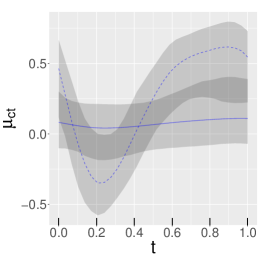
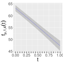
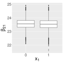
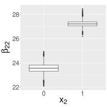
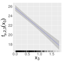
Concerning the mean regression models, results in the form of posterior means and credible intervals are presented in the Figure of the supplementary material. Covariate (gender) has little to no effect on the means of three cognitive function responses but it has an important effect on the mean of depressive symptomatology, indicating that males have, on average, less symptoms than females. Further, covariate (education) has important effects on the means of the responses relating to cognitive function, with those who graduated from primary school having higher mean cognitive function scores. In addition, appears to have no effect on mean depressive symptomatology. Covariates (age) and (time) have negative linear (or almost linear) associations with the means of the responses that relate to cognitive function. Furthermore, has a more complex than linear relationship with mean depressive symptomatology, but, due to the high uncertainty, this relationship could also be seen as flat. Lastly, has positive linear association with the mean of fourth response, indicating that the average depressive symptomatology increases with time. Visually, the covariates have simple relationships with the mean responses. This can also be confirmed by the small number of regression coefficients that are selected to fit the mean functions: of the , on average, or were selected during MCMC sampling.
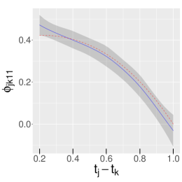
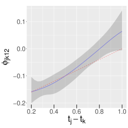
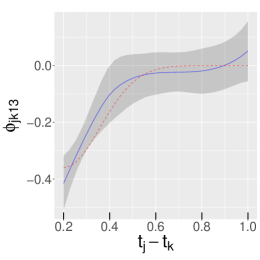
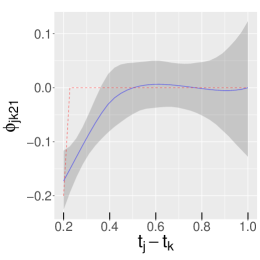
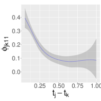
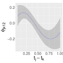
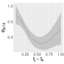
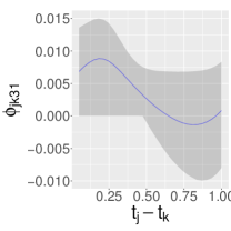
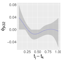
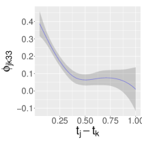
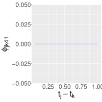
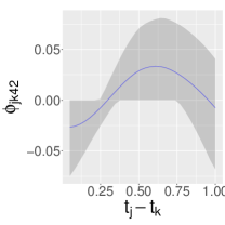
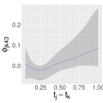
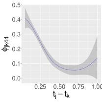
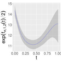
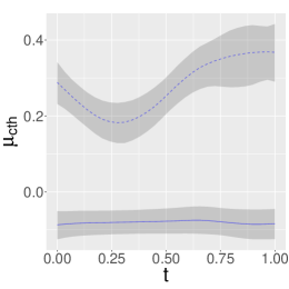
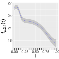
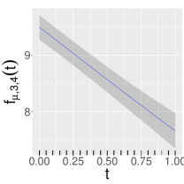
Results on the autoregressive coefficient regression models are shown in Figure 4. Recalling the discussion around (12), the fitted models presented in the diagonal of Figure 4 correspond to the coefficients for predicting responses based on passed observations on the same response. These 4 curves have similar shapes: they start from around to and they decrease towards . Based on univariate data analyses, Pan & MacKenzie, (2006) and Papageorgiou, (2012) reported similar curves. The remaining plots include a variety of fitted curves: complex and clearly important (such as and ), complex but not very important (such as and ) and flat at 0 (such as and ). For fitting these curves, of the regression coefficients, on average, or were selected during MCMC sampling.
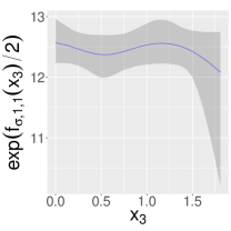
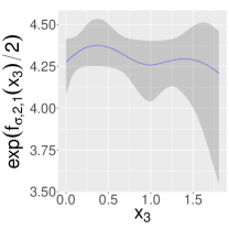
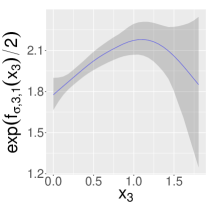
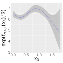
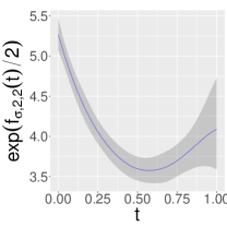
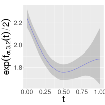
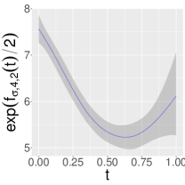
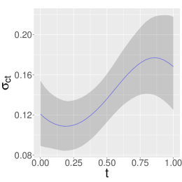
Results relating to innovation standard deviations are displayed in Figure 5. The first row shows almost flat fitted curves and , and more complex fitted curves and . The four fitted curves , shown in the second row of Figure 5, have similar shapes: they decrease as increases and they are characterized by increasing uncertainty as increases. For fitting these curves, of the regression coefficients, on average, or were selected during MCMC sampling.
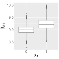
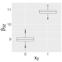
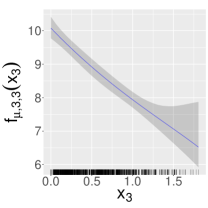
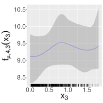
Figure 6 shows the fitted models of the parameters of the innovation correlation matrices. The first plot shows the clustering structure that the MCMC sampler visited most often: for of the MCMC samples, two clusters were formed, the first being (denoted by the darker colour on the plot) while the second being (denoted by the lighter colour). While this clustering was obtained by a ‘grouped correlations’ model, it is also compatible with the ‘grouped variables’ model, the first cluster consisting of variables (the results on the cognitive tests) and the second consisting of variable (the test result on depressive symptomatology). The other 2 plots in the Figure show the fitted curves for , and . The fitted curve starts at around , decreases below and then increases to just below . The fitted curve is much simpler: it is constant just below for all time points. For fitting these curves, of the regression coefficients, on average, or were selected during MCMC sampling. The fitted smooth curve for is shown in the third plot of Figure 6. For fitting this curve, of the regression coefficients, on average, or were selected during MCMC sampling.
Hence, overall, for fitting the unique elements of the covariance matrix, the model selects, on average, of the available parameters, per MCMC iteration.
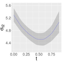
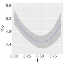
We conclude this section by providing an interpretation of the results in terms of the elements of the covariance matrix of the 4 responses. To do so, we construct two covariance matrices based on the sampled parameter values, both for time points and for equal to the lower and upper quartiles of age. With these choices we can examine the effects of time and age on the elements of . For every iteration of the MCMC sampler (that is not discarded), we first obtain the innovation variances from (50). Based on these and on the sampled correlation matrices , using (23), we reconstruct the innovation covariance matrices . Further, we obtain the autoregressive coefficients from (49), and based on these we construct the generalized autoregressive matrices , which, in turn, give us the matrix in (11). Lastly we rearrange (1) to obtain . This process results in realizations of the covariance matrices that correspond to and . Results are shown in Figures (7), (8) and (9).
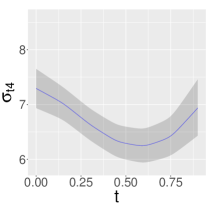
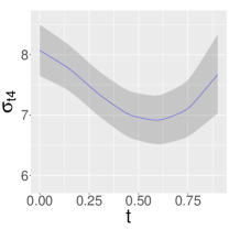
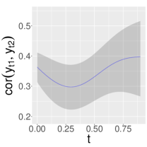
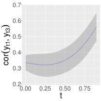
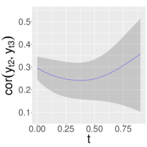
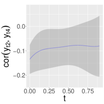
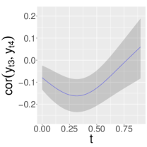
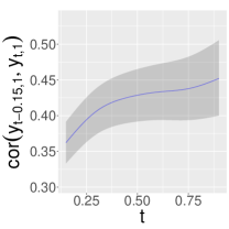
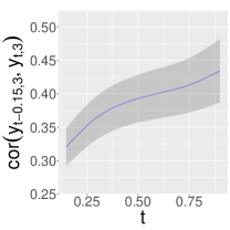
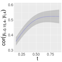
First, Figure (7) shows the posterior means and credible intervals for the standard deviations of and over time. The standard deviations of and have similar shapes as the ones for and , and hence they are omitted. We can see that in all plots the standard deviations first decrease and then increase with time, . The first two plots display the standard deviation of for and , respectively. We can see that age has no effect on the standard deviation of . However, it does have an effect on the standard deviation of as the curve in the fourth plot, when compared with that in the third plot, is shifted upwards. Further, Figure (8) shows how the correlations among responses evolve over time. We can see that some of the correlations exhibit an increasing trend (cor), others first decrease and then increase (cor, cor, and cor), while others are mostly flat (cor and cor). Lastly, Figure (9) displays autocorrelations at lag over time. These autocorrelations can be seen to be increasing over time.
 |
 |
 |
 |
 |
 |
 |
 |
 |
 |
 |
 |
 |
 |
 |
 |
 |
 |
 |
 |
 |
 |
 |
 |
 |
 |
 |
 |
 |
 |
 |
 |
 |
 |
 |
 |
 |
 |
 |
 |
 |
6 Discussion
The article describes a Bayesian framework for the analysis of multivariate longitudinal Gaussian responses, with nonparametric models for the means, the elements of the generalized autoregressive matrices, the elements of the innovation variance matrices, and the parameters of the innovation correlation matrices. The use of spike-slab priors is important here as it allows for automatic variable selection and function regularization, simultaneously in the submodels. Further, it obviates the need for model selection based on information criteria, see e.g. Pan & Mackenzie, (2003), and it allows for the uncertainty in the model choice to propagate in the model parameter estimates. In addition, the automatic variable selection allows each regression equation to have its own set of covariates. For example, looking back at (48), it may appear that the responses have the same mean model. However, the binary indicators for variable selection allow each response to have its own mean model. The same is true for the autoregressive coefficients and innovation variances.
The major assumption of the framework is that the errors have a multivariate Gaussian distribution. It is worthwhile to relax this assumption, and to that end, in future work, we will be exploring the use of the multivariate skew-normal distribution (Azzalini & Valle,, 1996).
7 Supplementary material I: MCMC algorithm
Here we provide all details of the MCMC sampler of the three correlation models. We note that for all steps that involve tuning parameters, the values of these are chosen adaptively (Roberts & Rosenthal,, 2009) to achieve an acceptance probability of (Roberts & Rosenthal,, 2001).
7.1 MCMC algorithm for the common correlations model
Starting from the common correlations model, the algorithm proceeds as follows:
-
1.
The elements of are updated in random order and in blocks of random size (Chan et al.,, 2006). Let be a block of elements of . The proposed value for is obtained from its prior with the remaining elements of , denoted by , kept at their current value. The proposal pmf is obtained from the binomial prior in (34) with integrated out
where denotes the length of i.e. the size of the block. For this proposal pmf, the acceptance probability of the Metropolis-Hastings move reduces to the ratio of the likelihoods in (40)
where superscripts and denote proposed and currents values respectively.
-
2.
Parameter is updated from the marginal (40) and the IG prior
To sample from the above, we utilize a normal approximation. Let . We utilize a normal proposal density , where is the mode of found using a Newton-Raphson algorithm, is the second derivative of evaluated at the mode, and is a tuning parameter. With superscripts and denoting proposed and currents values, the acceptance probability is the minimum between one and
-
3.
Pairs are updated simultaneously. Similarly to the updating of , the elements of are updated in random order and in blocks of random size. Let denote a block. Blocks and the whole vector are generated simultaneously. As was mentioned by Chan et al., (2006), generating the whole vector , instead of subvector , is necessary in order to make consistent with the proposed value of .
Generating the proposed value for is done in a similar way as was done for . Let denote the proposed value of . Next, we describe how the proposed vale for is obtained. To avoid clutter, proposed values will be denoted by the simpler . The development that follows is in the spirit of Chan et al., (2006) who built on the work of Gamerman, (1997).
Let denote the current value of the posterior mean of . Define the current squared residuals
These have an approximate distribution, where . The latter defines a Gamma generalized linear model (GLM) for the squared residuals with mean , which, utilizing a -link, can be thought of as Gamma GLM with an offset term: . Given , the proposal density for is derived utilizing the one step iteratively reweighted least squares algorithm. This proceeds as follows. First define the transformed observations
where superscript denotes current values. Further, let denote the vector of .
Next we define
where is a submatrix of that considers only the columns that pertain to the th effect. The proposed value is obtained from the multivariate normal distribution , where is a tuning parameter.
Let denote the proposal density for taking a step in the reverse direction, from model to . Then the acceptance probability of the pair is
where the determinants, for centred variables, are equal to one, otherwise, the ratio of the determinants may be computed as .
-
4.
The full conditional of is given by
where denotes either the IG or half-normal prior. We follow a random walk algorithm obtaining proposed values , where is a tuning parameter. Proposed values are accepted with probability , which reduces to
-
5.
Concerning parameter , the full conditional that corresponds to the IG prior is another inverse Gamma density IG.
The full conditional that corresponds to the half-normal prior is
We obtain proposed values from , where denotes the current value and denotes a tuning parameter. Proposed values are accepted with probability .
- 6.
-
7.
Pairs are updated simultaneously. Let denote a randomly chosen block of . The block and the whole of are updated simultaneously. Proposed values for are obtained from its prior, in a similar way as was done for . Now, to obtain a proposal for , note that the full conditional of , as obtained from its normal prior and the likelihood that corresponds to (39), is
where is a diagonal matrix with diagonal elements equal to , each having multiplicity equal to the length of . We use as proposal the conditional of given all other elements of , denoted by . Then, the acceptance probability of the pair is
-
8.
For parameter the full conditional that corresponds to the IG prior is another inverse Gamma density, IG.
The full conditional that corresponds to the half-normal prior is
We obtain proposed values from , where is the current value and is a tuning parameter. Proposed values are accepted with probability .
-
9.
To sample from the full conditional of recall (41) and (38). We have
(51) where denotes the total number of observations at time point , , and .
To obtain a proposal density and sample from (51) we utilize the method of Zhang et al., (2006) and Liu & Daniels, (2006). We start by considering symmetric pd and otherwise unconstrained matrices in place of . These are assumed to have an inverse Wishart prior , with mean equal to the realization of from the previous iteration. Given the inverse Wishart prior on , we obtain the following easy to sample from inverse Wishart posterior
(52) We decompose into a diagonal matrix of variances , and a correlation matrix . The Jacobian associated with this transformation is . It follows that the joint density for is
(53) -
10.
To sample from the full conditional of , first write for the likelihood of (41). Further, the prior for , as derived from (44), is where . Hence, it is easy to show that the posterior is
(54) At iteration we sample utilizing as proposal the normal distribution that appears on the right of (54), ignoring the normalizing constants. The proposed is accepted with probability
This, as was argued by Liechty et al., (2004) and Liechty et al., (2009), for a small value of , can reasonably be assumed to be unity.
-
11.
The elements of are updated in random order and in blocks of random size. Let be such a block. The proposed value for is obtained from its prior with the remaining elements of , denoted by , kept at their current value, in a similar way as was done for . The acceptance probability reduces to the ratio of the likelihoods in (44)
where superscripts and denote proposed and currents values respectively.
-
12.
Vectors and are updated following a similar approach as that for step 3. The elements of are updated in random order and in blocks of random size. Let denote a block. Blocks and the whole vector are generated simultaneously. Generating the proposed value for is done in a similar way as was done for . Let denote the proposed value of . Next, we describe how the proposed vale for is obtained. Let denote the current value of the posterior mean of . Define the current squared residuals
. These will have an approximate distribution, where . The latter defines a Gamma generalized linear model (GLM) for the squared residuals with mean , which, utilizing a -link, can be thought of as Gamma GLM with an offset term: . Given the proposed value of , denoted by , the proposal density for is derived utilizing the one step iteratively reweighted least squares algorithm. This proceeds as follows. First define the transformed observations
where superscript denotes current values. Further, let denote the vector of .
Next we define
where is the design matrix without the intercept column. The proposed value is obtained from a multivariate normal distribution with mean and covariance , denoted as , where is a tuning parameter.
Let denote the proposal density for taking a step in the reverse direction, from model to . Then the acceptance probability of the pair is
-
13.
We update utilizing the marginal (44) and the either of the two prior specifications. The full conditional that corresponds to the IG prior is
where denotes the number of unique observational times and . The above is recognized as IG.
The full conditional that corresponds to the half-normal prior is
Proposed values are obtained from , where denotes the current value and is a tuning parameter. Proposed values are accepted with probability .
-
14.
Parameter is updated from the marginal (44) and the IG prior
To sample from the above, we utilize a normal approximation to it. Let . We utilize a normal proposal density where is the mode of , found using a Newton-Raphson algorithm, is the second derivative of evaluated at the mode, and is a tuning parameter. At iteration the acceptance probability is the minimum between one and
-
15.
Concerning parameter , the full conditional that corresponds to the IG prior is another inverse Gamma density IG.
The full conditional that corresponds to the half-normal prior is
We obtain proposed values , where denotes the current value and is a tuning parameter. Proposed values are accepted with probability .
-
16.
The sampler utilizes the marginal in (44) to improve mixing. However, if samples are required from the posterior of , they can be generated from
where is the non-zero part of .
7.2 MCMC algorithm for the grouped correlations model
The algorithm for the ‘grouped correlations’ model requires additional steps (the first below) and a modification to a step from the algorithm of the ‘common correlations’ model (the last one below). We describe these next.
-
1.
Update where is the number of correlations, and is the number of correlations allocated in the th cluster. Given , update the weights .
-
2.
To calculate the cluster assignment probabilities first define to be the profile of the correlation. Based on (43), we have the following posterior probability
Here matrix is diagonal of dimension with elements given by , and matrix has rows given by i.e. it is the subset of that corresponds to . Vector is imputed from its posterior, or if the cluster is empty from prior (36).
-
3.
We update concentration parameter using the method described by Escobar & West, (1995). With the prior, the posterior can be expressed as a mixture of two Gamma distributions
(55) where is the number of non-empty clusters, and
(56) Hence, the algorithm proceeds as follows: with and fixed at their current values, we sample from (56). Then, based on the same and the newly sampled value of , we sample a new from (55).
-
4.
A modification to step 12. of the previous algorithm is needed. Here, we calculate the squared residuals based on . Furthermore, function is needed for this step.
7.3 MCMC algorithm for the grouped variables model
The algorithm for the ‘grouped variables’ model differs from that of the ‘grouped correlations’ model in the calculation of the cluster assignment probabilities. Here, they are computed as follows. Recall that and let be the prior probability that a variable is assigned to cluster . We have the following posterior probability
8 Supplementary material II: Application
Here we provide the Figure that displays the effects of the covariates on the means of the responses.
 |
 |
 |
 |
 |
 |
 |
 |
 |
 |
 |
 |
 |
 |
 |
 |
References
- Anderson, (1973) Anderson, T. W. (1973). Asymptotically efficient estimation of covariance matrices with linear structure. The Annals of Statistics, 1(1), 135–141.
- Azzalini & Valle, (1996) Azzalini, A. & Valle, A. D. (1996). The multivariate skew-normal distribution. Biometrika, 83(4), 715–726.
- Barnard et al., (2000) Barnard, J., McCulloch, R., & Meng, X.-L. (2000). Modeling covariance matrices in terms of standard deviations and correlations, with application to shrinkage. Statistica Sinica, 10(4), 1281–1311.
- Chan et al., (2006) Chan, D., Kohn, R., Nott, D., & Kirby, C. (2006). Locally adaptive semiparametric estimation of the mean and variance functions in regression models. Journal of Computational and Graphical Statistics, 15(4), 915–936.
- Chiu et al., (1996) Chiu, T. Y. M., Leonard, T., & Tsui, K.-W. (1996). The matrix-logarithmic covariance model. Journal of the American Statistical Association, 91(433), 198–210.
- Daniels & Kass, (1999) Daniels, M. J. & Kass, R. E. (1999). Nonconjugate Bayesian estimation of covariance matrices and its use in hierarchical models. Journal of the American Statistical Association, 94(448), 1254–1263.
- Daniels & Pourahmadi, (2002) Daniels, M. J. & Pourahmadi, M. (2002). Bayesian analysis of covariance matrices and dynamic models for longitudinal data. Biometrika, 89(3), 553–566.
- Escobar & West, (1995) Escobar, M. D. & West, M. (1995). Bayesian density estimation and inference using mixtures. Journal of the American Statistical Association, 90, 577–588.
- Feng et al., (2016) Feng, S., Lian, H., & Xue, L. (2016). A new nested Cholesky decomposition and estimation for the covariance matrix of bivariate longitudinal data. Computational Statistics & Data Analysis, 102, 98 – 109.
- Ferguson, (1973) Ferguson, T. S. (1973). A Bayesian analysis of some nonparametric problems. The Annals of Statistics, 1(2), 209–230.
- Gamerman, (1997) Gamerman, D. (1997). Sampling from the posterior distribution in generalized linear mixed models. Statistics and Computing, 7(1), 57–68.
- George & McCulloch, (1997) George, E. I. & McCulloch, R. E. (1997). Approaches for Bayesian variable selection. Statistica Sinica, 7(2), 339–373.
- Hamilton, (1994) Hamilton, J. (1994). Time series analysis. Princeton, NJ: Princeton Univ. Press.
- Kim & Zimmerman, (2012) Kim, C. & Zimmerman, D. L. (2012). Unconstrained models for the covariance structure of multivariate longitudinal data. Journal of Multivariate Analysis, 107, 104–118.
- Kohli et al., (2016) Kohli, P., Garcia, T. P., & Pourahmadi, M. (2016). Modeling the Cholesky factors of covariance matrices of multivariate longitudinal data. Journal of Multivariate Analysis, 145, 87 – 100.
- Lee et al., (2020) Lee, K., Cho, H., Kwak, M.-S., & Jang, E. J. (2020). Estimation of covariance matrix of multivariate longitudinal data using modified Choleksky and hypersphere decompositions. Biometrics, 76(1), 75–86.
- Leng et al., (2010) Leng, C., Zhang, W., & Pan, J. (2010). Semiparametric mean–covariance regression analysis for longitudinal data. Journal of the American Statistical Association, 105(489), 181–193.
- Letenneur et al., (1994) Letenneur, L., Commenges, D., Dartigues, J., & Barberger-Gateau, P. (1994). Incidence of dementia and Alzheimer’s disease in elderly community residents of south-western France. International Journal of Epidemiology, 23(6), 1256–1261.
- Liang et al., (2008) Liang, F., Paulo, R., Molina, G., Clyde, M. A., & Berger, J. O. (2008). Mixtures of g priors for Bayesian variable selection. Journal of the American Statistical Association, 103(481), 410–423.
- Liechty et al., (2004) Liechty, J. C., Liechty, M. W., & Müller, P. (2004). Bayesian correlation estimation. Biometrika, 91(1), 1–14.
- Liechty et al., (2009) Liechty, M. W., Liechty, J. C., & Müller, P. (2009). The shadow prior. Journal of Computational and Graphical Statistics, 18(2), 368–383.
- Lin & Pan, (2013) Lin, H. & Pan, J. (2013). Nonparametric estimation of mean and covariance structures for longitudinal data. Canadian Journal of Statistics, 41(4), 557–574.
- Liu & Daniels, (2006) Liu, X. & Daniels, M. J. (2006). A new algorithm for simulating a correlation matrix based on parameter expansion and reparameterization. Journal of Computational and Graphical Statistics, 15(4), 897–914.
- Pan & Mackenzie, (2003) Pan, J. & Mackenzie, G. (2003). On modelling mean-covariance structures in longitudinal studies. Biometrika, 90(1), 239–244.
- Pan & MacKenzie, (2006) Pan, J. & MacKenzie, G. (2006). Regression models for covariance structures in longitudinal studies. Statistical Modelling, 6(1), 43–57.
- Papageorgiou, (2012) Papageorgiou, G. (2012). Restricted maximum likelihood estimation of joint mean-covariance models. Canadian Journal of Statistics, 40(2), 225–242.
- Papageorgiou, (2018) Papageorgiou, G. (2018). BNSP: an R package for fitting Bayesian semiparametric regression models and variable selection. The R Journal, 10(2), 526–548.
- Papageorgiou, (2020) Papageorgiou, G. (2020). BNSP: Bayesian Non- And Semi-Parametric Model Fitting. R package version 2.1.5.
- Papageorgiou & Marshall, (2020) Papageorgiou, G. & Marshall, B. C. (2020). Bayesian semiparametric analysis of multivariate continuous responses, with variable selection. Journal of Computational and Graphical Statistics, 0(0), 1–14.
- Philipps et al., (2014) Philipps, V., Amieva, H., Andrieu, S., Dufouil, C., Berr, C., Dartigues, J. F., Jacqmin-Gadda, H., & Proust-Lima, C. (2014). Normalized mini-mental state examination for assessing cognitive change in population-based brain aging studies. Neuroepidemiology, 43, 15–25.
- Pourahmadi, (1999) Pourahmadi, M. (1999). Joint mean-covariance models with applications to longitudinal data: Unconstrained parameterisation. Biometrika, 86(3), 677–690.
- Pourahmadi, (2000) Pourahmadi, M. (2000). Maximum likelihood estimation of generalised linear models for multivariate normal covariance matrix. Biometrika, 87(2), 425–435.
- Pourahmadi, (2007) Pourahmadi, M. (2007). Cholesky decompositions and estimation of a covariance matrix: Orthogonality of variance-correlation parameters. Biometrika, 94(4), 1006–1013.
- Proust-Lima et al., (2020) Proust-Lima, C., Philipps, V., Diakite, A., & Liquet, B. (2020). lcmm: Extended Mixed Models Using Latent Classes and Latent Processes. R package version: 1.9.2.
- Roberts & Rosenthal, (2001) Roberts, G. O. & Rosenthal, J. S. (2001). Optimal scaling for various Metropolis-Hastings algorithms. Statistical Science, 16(4), 351–367.
- Roberts & Rosenthal, (2009) Roberts, G. O. & Rosenthal, J. S. (2009). Examples of adaptive MCMC. Journal of Computational and Graphical Statistics, 18(2), 349–367.
- Sethuraman, (1994) Sethuraman, J. (1994). A constructive definition of Dirichlet priors. Statistica Sinica, 4, 639–650.
- Xu & Mackenzie, (2012) Xu, J. & Mackenzie, G. (2012). Modelling covariance structure in bivariate marginal models for longitudinal data. Biometrika, 99(3), 649–662.
- Zellner, (1962) Zellner, A. (1962). An efficient method of estimating seemingly unrelated regressions and tests for aggregation bias. Journal of the American Statistical Association, 57(298), 348–368.
- Zellner, (1986) Zellner, A. (1986). On assessing prior distributions and Bayesian regression analysis with g-prior distributions. In P. Goel & Zellner (Eds.), Bayesian Inference and Decision Techniques: Essays in Honor of Bruno de Finetti (pp. 233–243).: Elsevier Science Publishers.
- Zhang & Leng, (2012) Zhang, W. & Leng, C. (2012). A moving average Cholesky factor model in covariance modelling for longitudinal data. Biometrika, 99(1), 141–150.
- Zhang et al., (2015) Zhang, W., Leng, C., & Tang, C. Y. (2015). A joint modelling approach for longitudinal studies. Journal of the Royal Statistical Society: Series B (Statistical Methodology), 77(1), 219–238.
- Zhang et al., (2006) Zhang, X., Boscardin, J. W., & Belin, T. R. (2006). Sampling correlation matrices in Bayesian models with correlated latent variables. Journal of Computational and Graphical Statistics, 15(4), 880–896.