A new asymptotic representation and inversion method for the Student’s $t$ distribution

Abstract

Some special functions are particularly relevant in applied probability and statistics. For example, the incomplete beta function is the cumulative central beta distribution. In this paper, we consider the inversion of the central Student’s-$t$ distribution which is a particular case of the central beta distribution. The inversion of this distribution functions is useful in hypothesis testing as well as for generating random samples distributed according to the corresponding probability density function. A new asymptotic representation in terms of the complementary error function, will be one of the important ingredients in our analysis. As we will show, this asymptotic representation is also useful in the computation of the distribution function. We illustrate the performance of all the obtained approximations with numerical examples.

1 Introduction

There is a very close relationship between some special functions and some of the most popular distribution functions in statistics. For example, the incomplete beta function (Paris:2010:INC, , §8.17) is the central beta distribution. Particular cases include other well-known distributions such as the geometric, binomial, negative binomial or the central Student’s-$t$ distribution. Therefore, standard methods for the computation and inversion of special functions Gil:2007:NSF can also be applied to evaluate and invert distribution functions. The problem of inversion appears, for example, when computing percentage points of the distribution functions; also, it is closely related to the generation of random variates from a continuous probability density function needed, for example, in Monte Carlo or quasi-Monte Carlo methods.

We have considered the central beta distribution in a previous publication Gil:2017:IBE . In this paper, we focus on the computation and inversion of the central Student’s-$t$ distribution, which has multiple applications in science and engineering (for an application in physics, see for example Rover:2011:RSD ). As we mentioned before, this distribution function is a particular case of the central beta distribution but which requires particular analysis. An asymptotic representation in terms of the complementary error function, will play a key role in our analysis. The performance of the approximations obtained will be illustrated with numerical examples.

There is a vast literature on Student’s $t$ distribution. An extensive overview can be found at Johnson:1995:CUD ; see also the references contained therein. For an historical account and the origin of this distribution, we refer to Zabell:2008:OAA . For a generalization from the viewpoint of special functions, see Koepf:2006:GSD .

Some useful expressions for the analysis of the central Student’s-t distribution are:

•

a) Probability density function:

$$f_{n}(t)=\frac{\Gamma\left(\frac{1}{2}n+\frac{1}{2}\right)}{\sqrt{n\pi}\,\Gamma\left(\frac{1}{2}n\right)}\left(1+\frac{t^{2}}{n}\right)^{-\frac{1}{2}n-\frac{1}{2}}=\frac{1}{\sqrt{n}\,B\left(\frac{1}{2},\frac{1}{2}n\right)}\left(1+\frac{t^{2}}{n}\right)^{-\frac{1}{2}n-\frac{1}{2}},$$ (1.1)

where $t\in{\mathbb{R}}$ and $B(p,q)$ is the Beta integral; $n>0$, not necessarily an integer.

•

b) Cumulative distribution function:

$$F_{n}(x)=\int_{-\infty}^{x}f_{n}(t)\,dt,\quad x\in\mathbb{R}.$$ (1.2)

•

c) Incomplete beta function:

$$I_{x}(p,q)=\frac{1}{B(p,q)}\int_{0}^{x}t^{p-1}(1-t)^{q-1}\,dt,\quad B(p,q)=\frac{\Gamma(p)\Gamma(q)}{\Gamma(p+q)}.$$ (1.3)

From the integral representation, we have:

$$I_{x}(p,q)=1-I_{1-x}(q,p).$$ (1.4)

•

d) Cumulative distribution function in terms of the incomplete beta function:

$$F_{n}(x)=\left\{\begin{array}[]{ll}\frac{1}{2}+\frac{1}{2}I_{\frac{x^{2}}{n+x^{2}}}\left(\frac{1}{2},\frac{1}{2}n\right)=1-\frac{1}{2}I_{\frac{n}{n+x^{2}}}\left(\frac{1}{2}n,\frac{1}{2}\right),&{\rm if\ }x\geq 0,\\ \frac{1}{2}-\frac{1}{2}I_{\frac{x^{2}}{n+x^{2}}}\left(\frac{1}{2},\frac{1}{2}n\right)=\frac{1}{2}I_{\frac{n}{n+x^{2}}}\left(\frac{1}{2}n,\frac{1}{2}\right),&{\rm if\ }x\leq 0.\\ \end{array}\right.$$ (1.5)

•

e) Cumulative distribution function in terms of the Gauss hypergeometric functions:

$$F_{n}(x)=\left\{\begin{array}[]{ll}\displaystyle{{{\lower 2.58334pt\hbox{$\scriptstyle 1$}}\over{\raise 3.01385pt\hbox{$\scriptstyle 2$}}}+\frac{x}{\sqrt{n}\,B\left(\frac{1}{2},\frac{1}{2}n\right)}}{}_{2}F_{1}\left(\begin{array}[]{c}\begin{array}[]{c}\hskip-10.0pt\frac{1}{2},\frac{1}{2}n+\frac{1}{2}\end{array}\\ \begin{array}[]{c}\hskip-10.0pt\frac{3}{2}\end{array}\end{array}\hskip-8.0pt;\,-\frac{x^{2}}{n}\right),&{\rm if\ }x\in\mathbb{R},\\ 1-\displaystyle{\frac{(1-y)^{\frac{1}{2}n}y^{-\frac{1}{2}}}{nB\left(\frac{1}{2},\frac{1}{2}n\right)}{}_{2}F_{1}\left(\begin{array}[]{c}\begin{array}[]{c}\hskip-10.0pt1,\frac{1}{2}\end{array}\\ \begin{array}[]{c}\hskip-10.0pt\frac{1}{2}n+1\end{array}\end{array}\hskip-8.0pt;\,-\frac{n}{x^{2}}\right),}&{\rm if\ }x\geq 0,\\ \displaystyle{\frac{(1-y)^{\frac{1}{2}n}y^{-\frac{1}{2}}}{nB\left(\frac{1}{2},\frac{1}{2}n\right)}{}_{2}F_{1}\left(\begin{array}[]{c}\begin{array}[]{c}\hskip-10.0pt1,\frac{1}{2}\end{array}\\ \begin{array}[]{c}\hskip-10.0pt\frac{1}{2}n+1\end{array}\end{array}\hskip-8.0pt;\,-\frac{n}{x^{2}}\right),}&{\rm if\ }x\leq 0,\\ \end{array}\right.$$ (1.6)

where $y=x^{2}/(n+x^{2})$. The first formula in (1.6) is given in Amos:1964:RBD , the other ones follow from well-known relations between the incomplete beta function and the hypergeometric function; see (Paris:2010:INC, , §8.17(ii)).

2 Asymptotic expansion of the Student’s $t$ cumulative distribution function

The second and third representation in (1.6) can be used for large values of $n$ by using the standard power series of the hypergeometric functions. It is not necessarily that $x^{2}>n$, but a condition $x^{2}/n={\cal O}(1)$ is needed. To obtain a large-$n$ asymptotic representation, whether or not $x$ is large, we use a method that we have used for other cumulative distribution functions; see (Temme:2015:AMI, , Chapter 36).

We use in (1.1) the substitution $t=s\sqrt{n}$. This gives

$$\begin{array}[]{@{}r@{\;}c@{\;}l@{}}F_{n}(x)&=&\displaystyle{\frac{1}{\sqrt{n}\,B\left(\frac{1}{2},\frac{1}{2}n\right)}\int_{-\infty}^{x}\left(1+\frac{t^{2}}{n}\right)^{-\frac{1}{2}n-\frac{1}{2}}\,dt}\\[8.0pt] &=&\displaystyle{\frac{1}{B\left(\frac{1}{2},\frac{1}{2}n\right)}\int_{-\infty}^{x/\sqrt{n}}\left(1+s^{2}\right)^{-\frac{1}{2}n-\frac{1}{2}}\,ds.}\end{array}$$ (2.1)

We write $u^{2}=\ln(1+s^{2})$, with the condition ${\rm sign}(u)={\rm sign}(s)$, and obtain

$$F_{n}(x)=\frac{1}{B\left(\frac{1}{2},\frac{1}{2}n\right)}\int_{-\infty}^{\xi}e^{-\frac{1}{2}nu^{2}}g(u)\,du,$$ (2.2)

where

$$g(u)=\sqrt{\frac{u^{2}}{1-e^{-u^{2}}}},\quad\xi^{2}=\ln\left(1+\frac{x^{2}}{n}\right),\quad{\rm sign}(\xi)={\rm sign}(x).$$ (2.3)

Using the method of (Temme:2015:AMI, , §36.1) we find that $F_{n}(x)$ can be written in the form

$$F_{n}(x)={{\lower 2.58334pt\hbox{$\scriptstyle 1$}}\over{\raise 3.01385pt\hbox{$\scriptstyle 2$}}}{\rm erfc}\left(-\xi\sqrt{n/2}\right)-\frac{e^{-\frac{1}{2}n\xi^{2}}}{\sqrt{2\pi n}\,\beta(n)}B_{n}(\xi),\quad\beta(n)=\sqrt{\frac{n}{2\pi}}\,B\left({{\lower 2.58334pt\hbox{$\scriptstyle 1$}}\over{\raise 3.01385pt\hbox{$\scriptstyle 2$}}},{{\lower 2.58334pt\hbox{$\scriptstyle 1$}}\over{\raise 3.01385pt\hbox{$\scriptstyle 2$}}}n\right),$$ (2.4)

where we have introduced the complementary error function

$${\rm erfc}\,z=\frac{2}{\sqrt{\pi}}\int_{z}^{\infty}e^{-t^{2}}\,dt.$$ (2.5)

The function $B_{n}(\xi)$ has the asymptotic expansion

$$B_{n}(\xi)\sim\sum_{k=0}^{\infty}\frac{C_{k}(\xi)}{n^{k}},\quad n\to\infty,\quad\xi\in\mathbb{R},$$ (2.6)

where the coefficients follow from the recursive scheme

$$C_{k}(\xi)=\frac{g_{k}(\xi)-g_{k}(0)}{\xi},\quad g_{k+1}(u)=\frac{d}{du}\frac{g_{k}(u)-g_{k}(0)}{u},$$ (2.7)

with $g_{0}(u)=g(u)$ defined in (2.3). The first coefficients are

$$\begin{array}[]{@{}r@{\;}c@{\;}l@{}}C_{0}(\xi)&=&\displaystyle{\frac{g(\xi)-1}{\xi}},\\[8.0pt] C_{1}(\xi)&=&\displaystyle{-\frac{4g(\xi)^{3}-4g(\xi)\xi^{2}+\xi^{2}-4}{4\xi^{3}}},\\[8.0pt] C_{2}(\xi)&=&\displaystyle{\frac{96g(\xi)^{5}-128g(\xi)^{3}\xi^{2}+32g(\xi)\xi^{4}-\xi^{4}+8\xi^{2}-96}{32\xi^{5}}}.\end{array}$$ (2.8)

The function $\beta(n)$ has the expansion

$$\beta(n)\sim\sum_{k=0}^{\infty}\frac{D_{k}}{n^{k}},\quad n\to\infty,\quad D_{k}=g_{k}(0).$$ (2.9)

The first coefficients are

$$D_{0}=1,\quad D_{1}={{\lower 2.58334pt\hbox{$\scriptstyle 1$}}\over{\raise 3.01385pt\hbox{$\scriptstyle 4$}}},\quad D_{2}={{\lower 2.58334pt\hbox{$\scriptstyle 1$}}\over{\raise 3.01385pt\hbox{$\scriptstyle 32$}}},\quad D_{3}=-{{\lower 2.58334pt\hbox{$\scriptstyle 5$}}\over{\raise 3.01385pt\hbox{$\scriptstyle 128$}}}.$$ (2.10)

These coefficients can be expressed in terms of the coefficients $a_{k}$ of $\displaystyle{g(u)=\sum_{k=0}^{\infty}a_{k}u^{k}}$. We have (see (Temme:2015:AMI, , Remark 36.2))

$$D_{k}=\left({{\lower 2.58334pt\hbox{$\scriptstyle 1$}}\over{\raise 3.01385pt\hbox{$\scriptstyle 2$}}}\right)^{k}2^{k}a_{2k},\quad k=0,1,2,\ldots\,.$$ (2.11)

Examples of the performance of the expansion (2.4) for three values of $n$ ($n=10,\,100,\,1000$) are shown in Figure 1. Five $C_{k}$coefficients in the series (2.6) have been considered in the computations. Relative errors in comparison to the values of the distribution function given in (1.6) computed with Maple.

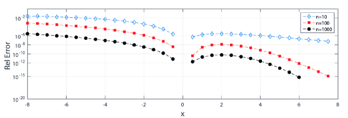
Figure 1: Relative errors obtained when computing the Student’s $t$ cumulative distribution function using the expansion (2.4).

3 Inversion of the Student’s $t$ cumulative distribution function

The inversion problem is: find $x$ that satisfies the equation

$$F_{n}(x)=p,\quad 0<p<1.$$ (3.1)

We consider three different approaches, the first one is for small values of $p-\frac{1}{2}$, which will give small values of $x$. The second method is for small values of $p$, which gives large negative values $x$. Thirdly we use the uniform approximation of §2, which will be valid for a large range of $x$, including the values near $x=0$.

3.1 Inversion for small values of $p-\frac{1}{2}$

We use the first representation in (1.6), and write the inversion problem in the form

$$x\sum_{k=0}^{\infty}c_{k}x^{2k}=q,\quad q=\left(p-{{\lower 2.58334pt\hbox{$\scriptstyle 1$}}\over{\raise 3.01385pt\hbox{$\scriptstyle 2$}}}\right)\sqrt{n}\,B\left({{\lower 2.58334pt\hbox{$\scriptstyle 1$}}\over{\raise 3.01385pt\hbox{$\scriptstyle 2$}}},{{\lower 2.58334pt\hbox{$\scriptstyle 1$}}\over{\raise 3.01385pt\hbox{$\scriptstyle 2$}}}n\right),$$ (3.2)

and the $c_{k}$ follow from the coefficients of the hypergeometric function:

$$c_{k}=\frac{\left(\frac{1}{2}\right)_{k}\left(\frac{1}{2}n+\frac{1}{2}\right)_{k}}{k!\,\left(\frac{3}{2}\right)_{k}}\frac{(-1)^{k}}{n^{k}}.$$ (3.3)

The solution of the equation in (3.1) has the expansion $\displaystyle{x=q\sum_{k=0}^{\infty}x_{k}q^{2k}}$, and the first coefficients are

$$\begin{array}[]{@{}r@{\;}c@{\;}l@{}}x_{0}&=&1,\quad\displaystyle{x_{1}=\frac{n+1}{6n},\quad x_{2}=\frac{(n+1)(7n+1)}{120n^{2}},}\\[8.0pt] x_{3}&=&\displaystyle{\frac{(n+1)(127n^{2}+8n+1)}{5040n^{3}},\quad x_{4}=\frac{(n+1)(4369n^{3}-537n^{2}+135n+1)}{362880n^{4}}.}\end{array}$$ (3.4)

We see that the shown coefficients are bounded for large values of $n$. Also, $q=\left(p-\frac{1}{2}\right)\sqrt{2\pi}\,\beta(n)$ (see (2.4)) with an expansion of $\beta(n)$ given in (2.9). This shows that the inversion considered here for small values of $\left(p-\frac{1}{2}\right)$ is rather well conditioned for large values of $n$. In (2) we show examples of the performance of the expansion (using the four terms given in (3.4)) for three values of $n$. The values of $p$ considered in the calculations are $p=\frac{1}{2}-\Delta$, for $\Delta=10^{-14}$, $2\times 10^{-12}$, $3\times 10^{-10}$, $4\times 10^{-8}$, $5\times 10^{-6}$, $6\times 10^{-4}$. The results obtained with the expansion have been compared with the Matlab function for the inversion of the central Student’s-t distribution (function tinv). As can be seen, a relative error better than $10^{-13}$ is obtained in all cases.

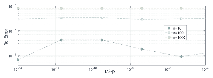
Figure 2: Performance of the expansion for small values of $p-\frac{1}{2}$ for three values of $n$. The five coefficients given in (3.4) for the expansion have been considered in the computations.

Remark 1

By using the definition in (1.2), it is easily verified that the function $F_{n}(x)$ becomes for $n=1$

$$F_{1}(x)=\frac{1}{2}+\frac{1}{\pi}\arctan\,x,$$ (3.5)

and for the inversion problem $F_{n}(x)=p$ we have $q=\left(p-\frac{1}{2}\right)\pi$. The equation to be inverted becomes $\arctan x=q$, with solution $x=\tan q$. The shown coefficients in (3.4) correspond with those of the expansion $x=q+\frac{1}{3}q^{3}+\frac{2}{15}q^{5}+\dots$. This expansion converges for $0<p<1$.

3.2 High-order iteration

It should be mentioned that it is also possible to obtain numerical approximations for the inversion problem for small values of $p-\frac{1}{2}$ using the fixed point iterations giving sharp error bounds for the central beta distribution described in Gil:2017:IBE . For example, iterating the fixed point iterations $y=g(y)$ or $y=h(y)$ where

$$\begin{array}[]{l}g(y)=\left(2(p-\frac{1}{2})B(\frac{1}{2},\frac{1}{2}n)(\frac{1}{2}-(\frac{1}{2}+\frac{1}{2}n)y)\right)^{2}(1-y)^{-n},\\[8.0pt] h(y)=225\frac{{\raise 1.80835pt\hbox{$\displaystyle\left(p-\frac{1}{2}\right)^{2}B\left(\frac{1}{2},\frac{1}{2}n\right)^{2}(1-y)^{-n}$}}}{{\lower 1.80835pt\hbox{$\displaystyle\left(y^{2}(n^{2}+4n+3)+5y(n+1)+15\right)^{2}$}}},\end{array}$$ (3.6)

starting from $y=0$, approximations to the values of $x$ in (3.1) are obtained with $x=\displaystyle\sqrt{\frac{{\raise 2.58334pt\hbox{$\displaystyle ny$}}}{{\lower 2.58334pt\hbox{$\displaystyle 1-y$}}}}$. As an example, using 2 iterations of the fixed point iteration $y=h(y)$ for $n=10$, $p=0.5+10^{-5}$ we find $x=0.00002569978035$ with a relative error $5\times 10^{-12}$. An explicit expression for the $x$ value obtained in the second iteration is

$$x=120\left(\frac{{\raise 2.58334pt\hbox{$\displaystyle nZ(1-(1/4)Z)^{-n}$}}}{{\lower 2.58334pt\hbox{$\displaystyle Z^{4}A_{4}+Z^{3}A_{3}+Z^{2}A_{2}+ZA_{1}+57600$}}}\right)^{1/2},$$ (3.7)

where $Z=\left(2(p-\frac{1}{2})B(\frac{1}{2},\frac{1}{2}n)\right)^{2}$ and

$$\begin{array}[]{l}A_{1}=-14400(1-(1/4)Z)^{-n}+9600n+9600,\\ A_{2}=880n^{2}+2720n+1840,\\ A_{3}=40n^{3}+200n^{2}+280n+120,\\ A_{4}=n^{4}+8n^{3}+22n^{2}+24n+9.\end{array}$$ (3.8)

This approximation can be also used for not so small values of $p-\frac{1}{2}$, as can be seen in Figure 3.

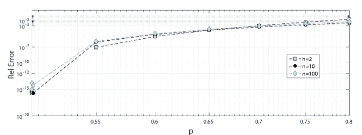
Figure 3: Relative errors obtained when using (3.7) to approximate the solution to the inversion problem (3.1) for $n=2,\,10,\,100$.

3.3 Inversion for small values of $p$

For this case we use the representation in the third line of (1.6) and introduce

$$\eta=\frac{n}{x^{2}},\quad\delta=\left(pnB\left({{\lower 2.58334pt\hbox{$\scriptstyle 1$}}\over{\raise 3.01385pt\hbox{$\scriptstyle 2$}}},{{\lower 2.58334pt\hbox{$\scriptstyle 1$}}\over{\raise 3.01385pt\hbox{$\scriptstyle 2$}}}n\right)\right)^{\frac{2}{n}}.$$ (3.9)

Then we can write the equation $F_{n}(x)=p$ in the form

$$\eta(1+\eta)^{\frac{1}{n}-1}S(\eta)^{\frac{2}{n}}=\delta,$$ (3.10)

where $S(\eta)$ is the standard power series of the hypergeometric function in the third line of (1.6) .

We see that for small values of $\delta$ the wanted variable $\eta$ behaves as $\eta\sim\delta$, and substituting the expansion

$$\eta=\sum_{k=1}^{\infty}\eta_{k}\delta^{k},$$ (3.11)

we find the following first few coefficients

$$\begin{array}[]{l}\eta_{1}=1,\quad\eta_{2}=\frac{{\raise 1.80835pt\hbox{$\displaystyle n+1$}}}{{\lower 1.80835pt\hbox{$\displaystyle n+2$}}},\quad\eta_{3}=\frac{{\raise 1.80835pt\hbox{$\displaystyle(n+1)\left(2n^{2}+9n+6\right)$}}}{{\lower 1.80835pt\hbox{$\displaystyle 2(n+2)^{2}(n+4)$}}},\\[8.0pt] \eta_{4}=\frac{{\raise 1.80835pt\hbox{$\displaystyle 3n^{6}+35n^{5}+134n^{4}+328n^{3}+1174n^{2}+2100n+1152$}}}{{\lower 1.80835pt\hbox{$\displaystyle 3n(n+2)^{3}(n+4)(n+6)$}}}.\\ \end{array}$$ (3.12)

When we have computed $\eta$, $x$ follows from (3.9): $x=-\sqrt{n/\eta}$.

Again, we see that the coefficients satisfy $\eta_{k}={\cal O}(1)$ for large values of $n$, which also happens for all coefficients that we have evaluated. The first 10 coefficients satisfy $\eta_{k}=1+{\cal O}(1/n)$ as $n\to\infty$. When $n$ is large, the only problem is that $\delta$ tends to 1, which for convergence of the series in (3.11) is a bad condition.

For example, when $p=10^{-8}$ and $n=10$, we have $\delta\doteq 0.038193186$. With 5 terms in the series in (3.11) we find $\eta\doteq 0.039576861$, giving $x\doteq-15.8956879$. Then, $F_{n}(x)=9.9999981\times 10^{-9}$, with relative error $1.92\times 10^{-7}$. For $n=25$ we find $\delta\doteq 0.281$, $x\doteq-8.0759$ and a relative error $0.011$. Other examples of the performance of the series for small values of $p$ are given in Table 1, where we show the values and relative errors obtained for $n=10$ and few values of $p$. The four coefficients given in (3.12) have been considered in the calculations. Since the Matlab function tinv seems to fail for very small values of $p$, the tests have been performed comparing with Maple.

$$\begin{array}[]{ccc}p&x&\mbox{Rel. Error}\\ \hline\cr 1\times 10^{-50}&-256452.5718769479&6.5\times 10^{-15}\\ 2\times 10^{-40}&-23927.87084268530&3.2\times 10^{-15}\\ 3\times 10^{-30}&-2297.706518629116&1.0\times 10^{-13}\\ 4\times 10^{-20}&-223.234400503956&1.1\times 10^{-09}\\ 5\times 10^{-10}&-21.62201646469524&1.2\times 10^{-05}\\ \end{array}$$

Table 1: Inversion values $x$ obtained (for $n=10$) using the series in (3.11) for small values of $p$. The coefficients given in (3.12) have been considered in the calculations. Relative errors in comparison to Maple, are also shown in the table.

Remark 2

When we take $n=1$ and use (3.5), the inversion problem becomes

$$x=-\cot(p\pi),\quad\eta=\tan^{2}(p\pi),\quad\delta=p^{2}\pi^{2},\quad 0<p<1.$$ (3.13)

The expansion in (3.11) becomes for $p<\frac{1}{2}$ and $\delta<\frac{1}{4}\pi^{2}$

$$\tan^{2}(p\pi)=\sum_{k=1}^{\infty}\eta_{k}\delta^{k},\quad\eta_{1}=1,\quad\eta_{2}={{\lower 2.58334pt\hbox{$\scriptstyle 2$}}\over{\raise 3.01385pt\hbox{$\scriptstyle 3$}}},\quad\eta_{3}={{\lower 2.58334pt\hbox{$\scriptstyle 17$}}\over{\raise 3.01385pt\hbox{$\scriptstyle 45$}}}.$$ (3.14)

These values of $\eta_{k}$ correspond with those given in (3.12) for $n=1$.

3.4 Inversion by using the uniform expansion

We use the representation given in (2.4) and first try to find $\xi$, then $x$ follows from the relation in (2.3). We assume that $n$ is large and use the asymptotic method as described in (Temme:2015:AMI, , §42.1) and in our papers Gil:2017:IBE , Gil:2019:NCB , Gil:2020:IBD .

Let $\xi_{0}$ satisfy the equation

$${{\lower 2.58334pt\hbox{$\scriptstyle 1$}}\over{\raise 3.01385pt\hbox{$\scriptstyle 2$}}}{\rm erfc}\left(-\xi_{0}\sqrt{n/2}\right)=p.$$ (3.15)

Then we assume for $\xi$ the expansion

$$\xi\sim\xi_{0}+\frac{\xi_{1}}{n}+\frac{\xi_{2}}{n^{2}}+\frac{\xi_{3}}{n^{3}}+\ldots,$$ (3.16)

where $\xi_{k}$ have to be determined. When we have this approximation $\xi$ we compute $x$ from (2.3).

From (3.1), (1) and (2.2) we find

$$\frac{dp}{d\xi_{0}}=\sqrt{\frac{n}{2\pi}}e^{-\frac{1}{2}n\xi_{0}^{2}},\quad\frac{dp}{d\xi}=\sqrt{\frac{n}{2\pi}}\frac{g(\xi)}{\beta(n)}e^{-\frac{1}{2}n\xi^{2}},$$ (3.17)

where $\beta(n)$ is defined in (2.4).

Dividing the two derivatives, we find

$$g(\xi)\frac{d\xi}{d\xi_{0}}=\beta(n)e^{\frac{1}{2}n(\xi^{2}-\xi_{0}^{2})},$$ (3.18)

We substitute the expansion given in (3.16), use $\beta(n)=1+{\cal O}(1/n)$, and obtain, considering equal large-order terms of $n$, the next term in the expansion:

$$g(\xi_{0})=e^{\xi_{0}\xi_{1}}\quad\Longrightarrow\quad\xi_{1}=\frac{1}{\xi_{0}}\ln g(\xi_{0}).$$ (3.19)

Because

$$g(u)=1+{{\lower 2.58334pt\hbox{$\scriptstyle 1$}}\over{\raise 3.01385pt\hbox{$\scriptstyle 4$}}}u^{2}+{{\lower 2.58334pt\hbox{$\scriptstyle 1$}}\over{\raise 3.01385pt\hbox{$\scriptstyle 96$}}}u^{4}+{\cal O}\left(u^{6}\right),$$ (3.20)

it follows that $\xi_{1}$ is well defined when $\xi_{0}$ tends to zero (that is, when $p\sim\frac{1}{2}$).

We can find higher-order terms $\xi_{j},j\geq 2,$ of the expansion in (3.16) using more coefficients in the asymptotic expansion of $\beta(n)$ (see (2.10)). Also, we need the expansion

$$g(\xi)=g(\xi_{0})+(\xi-\xi_{0})g^{\prime}(\xi_{0})+{{\lower 2.58334pt\hbox{$\scriptstyle 1$}}\over{\raise 3.01385pt\hbox{$\scriptstyle 2$}}}(\xi-\xi_{0})^{2}g^{\prime\prime}(\xi_{0})+\ldots.$$ (3.21)

By using (3.18) and algebraic manipulations we find a few other coefficients:

$$\begin{array}[]{@{}r@{\;}c@{\;}l@{}}\xi_{2}&=&-\Bigl{(}2g\xi\xi_{1}^{2}+4\left(g-\xi g^{\prime}\right)\xi_{1}+\xi g-4g^{\prime}\Bigr{)}/(4\xi^{2}g),\\[8.0pt] \xi_{3}&=&\Bigl{(}2\xi^{2}g^{2}\xi_{1}^{3}+\left(2\xi^{3}gg^{\prime\prime}-2\xi^{3}{g^{\prime}}^{2}-6\xi^{2}gg^{\prime}+8\xi g^{2}\right)\xi_{1}^{2}+\\ &&\left(12g+\xi^{2}g-16\xi g^{\prime}+4\xi^{2}g^{\prime\prime}\right)g\xi_{1}+\\ &&\xi g^{2}+4\xi gg^{\prime\prime}+2\xi{g^{\prime}}^{2}-\xi^{2}gg^{\prime}-12gg^{\prime}\Bigr{)}\Bigl{/}(4\xi^{4}g^{2}),\end{array}$$ (3.22)

where $\xi=\xi_{0}$ and $g$, $g^{\prime}$ and $g^{\prime\prime}$ are evaluated at $\xi_{0}$.

For small values of $\xi_{0}$ (that is, when $p\sim\frac{1}{2}$), we need expansions. We have

$$\begin{array}[]{@{}r@{\;}c@{\;}l@{}}\xi_{1}&=&\displaystyle{\ {{\lower 2.58334pt\hbox{$\scriptstyle 1$}}\over{\raise 3.01385pt\hbox{$\scriptstyle 4$}}}\xi_{0}-{{\lower 2.58334pt\hbox{$\scriptstyle 1$}}\over{\raise 3.01385pt\hbox{$\scriptstyle 48$}}}\xi_{0}^{3}+{{\lower 2.58334pt\hbox{$\scriptstyle 1$}}\over{\raise 3.01385pt\hbox{$\scriptstyle 5760$}}}\xi_{0}^{7}-{{\lower 2.58334pt\hbox{$\scriptstyle 1$}}\over{\raise 3.01385pt\hbox{$\scriptstyle 362880$}}}\xi_{0}^{11}+{{\lower 2.58334pt\hbox{$\scriptstyle 1$}}\over{\raise 3.01385pt\hbox{$\scriptstyle 19353600$}}}\xi_{0}^{15}+\ldots,}\\[8.0pt] \xi_{2}&=&\displaystyle{{{\lower 2.58334pt\hbox{$\scriptstyle 1$}}\over{\raise 3.01385pt\hbox{$\scriptstyle 32$}}}\xi_{0}-{{\lower 2.58334pt\hbox{$\scriptstyle 5$}}\over{\raise 3.01385pt\hbox{$\scriptstyle 192$}}}\xi_{0}^{3}+{{\lower 2.58334pt\hbox{$\scriptstyle 7$}}\over{\raise 3.01385pt\hbox{$\scriptstyle 2560$}}}\xi_{0}^{5}+{{\lower 2.58334pt\hbox{$\scriptstyle 1$}}\over{\raise 3.01385pt\hbox{$\scriptstyle 2560$}}}\xi_{0}^{7}-{{\lower 2.58334pt\hbox{$\scriptstyle 407$}}\over{\raise 3.01385pt\hbox{$\scriptstyle 5806080$}}}\xi_{0}^{9}-{{\lower 2.58334pt\hbox{$\scriptstyle 13$}}\over{\raise 3.01385pt\hbox{$\scriptstyle 1451520$}}}\xi_{0}^{11}+\ldots,}\\[8.0pt] \xi_{3}&=&\displaystyle{-{{\lower 2.58334pt\hbox{$\scriptstyle 5$}}\over{\raise 3.01385pt\hbox{$\scriptstyle 128$}}}\xi_{0}-{{\lower 2.58334pt\hbox{$\scriptstyle 11$}}\over{\raise 3.01385pt\hbox{$\scriptstyle 1536$}}}\xi_{0}^{3}+{{\lower 2.58334pt\hbox{$\scriptstyle 63$}}\over{\raise 3.01385pt\hbox{$\scriptstyle 10240$}}}\xi_{0}^{5}-{{\lower 2.58334pt\hbox{$\scriptstyle 823$}}\over{\raise 3.01385pt\hbox{$\scriptstyle 2580480$}}}\xi_{0}^{7}-{{\lower 2.58334pt\hbox{$\scriptstyle 5291$}}\over{\raise 3.01385pt\hbox{$\scriptstyle 23224320$}}}\xi_{0}^{9}+\ldots,}\\[8.0pt] \xi_{4}&=&\displaystyle{-{{\lower 2.58334pt\hbox{$\scriptstyle 21$}}\over{\raise 3.01385pt\hbox{$\scriptstyle 2048$}}}\xi_{0}+{{\lower 2.58334pt\hbox{$\scriptstyle 37$}}\over{\raise 3.01385pt\hbox{$\scriptstyle 2048$}}}\xi_{0}^{3}+{{\lower 2.58334pt\hbox{$\scriptstyle 179$}}\over{\raise 3.01385pt\hbox{$\scriptstyle 81920$}}}\xi_{0}^{5}-{{\lower 2.58334pt\hbox{$\scriptstyle 22711$}}\over{\raise 3.01385pt\hbox{$\scriptstyle 10321920$}}}\xi_{0}^{7}+\ldots,}\\[8.0pt] \xi_{5}&=&\displaystyle{{{\lower 2.58334pt\hbox{$\scriptstyle 399$}}\over{\raise 3.01385pt\hbox{$\scriptstyle 8192$}}}\xi_{0}+{{\lower 2.58334pt\hbox{$\scriptstyle 219$}}\over{\raise 3.01385pt\hbox{$\scriptstyle 32768$}}}\xi_{0}^{3}-{{\lower 2.58334pt\hbox{$\scriptstyle 3679$}}\over{\raise 3.01385pt\hbox{$\scriptstyle 327680$}}}\xi_{0}^{5}+\ldots,}\\[8.0pt] \xi_{6}&=&\displaystyle{{{\lower 2.58334pt\hbox{$\scriptstyle 869$}}\over{\raise 3.01385pt\hbox{$\scriptstyle 65536$}}}\xi_{0}-{{\lower 2.58334pt\hbox{$\scriptstyle 6877$}}\over{\raise 3.01385pt\hbox{$\scriptstyle 131072$}}}\xi_{0}^{3}+\ldots\ .}\end{array}$$ (3.23)

Example 1

We summarise the algorithmic steps for the inversion method. We take $n=10$, $p=0.44$ and two terms in the expansion in (3.16).

1. Compute $\xi_{0}$ from equation (1). We have $\xi_{0}\doteq-0.047746$.

2. Compute $\xi_{1}$ from equation (3.19) by using $g(u)$ defined in (2.3): $\xi_{1}\doteq-0.011933$.

3. Compute $\xi$ by using (3.16) with the information now available: $\xi\sim\xi_{0}+\xi_{1}/n\doteq-0.048934$.

4. Compute $x$ from equation (2.3). Because $\xi<0$, $x$ should be negative: $x\doteq-0.1548354$.

5. Verification: compute $F_{n}(x)$ by using the first line in (1.6): $F_{10}(x)\doteq 0.4400158$. Relative error: $0.000036$.

A test of the performance of the asymptotic inversion method for three values of $n$ using the expansion for small values of $\xi_{0}$ given in (3.23), can be seen in Figure 4. The terms of the expansion $\xi_{1},\xi_{2},\xi_{3},\xi_{4}$ given in (3.23) have been considered in the computations. For computing the inverse of the complementary error function needed to compute $\xi_{0}$ in we use the function inverfc given in Gil:2015:GCH . The relative errors obtained in comparison to the Matlab function tinv are shown in the figure.

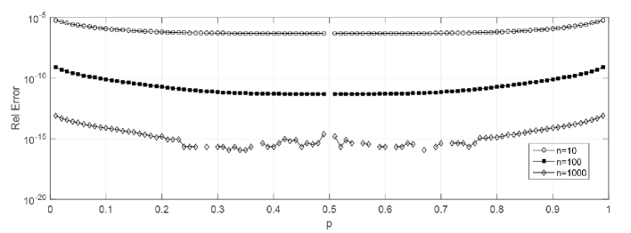
Figure 4: Performance of the asymptotic inversion method using four terms of the expansion for small values of $\xi_{0}$ given in (3.23). Three values of $n$ are considered in the computations.

4 Concluding remarks

We have presented approximations for the inversion problem (3.1) of the central Student-$t$ distributions. To obtain the approximations, different methods have been considered depending on the values of $p$. In particular, one of the key elements in our analysis was the use of an asymptotic representation of the distribution function in terms of the complementary error function. Numerical tests have shown that the approximations obtained are, in all cases, accurate. Also, they are easy to compute, which is an important advantage when using the inverse to generate random variates distributed according to central Student-$t$ probability density function.

References

• [1] D.E. Amos. Representations of the central and non-central $t$ distributions. Biometrika, 51:451–458, 1964.
• [2] A. Gil, J. Segura, and N. M. Temme. Numerical Methods for Special Functions. Society for Industrial and Applied Mathematics (SIAM), Philadelphia, PA, 2007.
• [3] A. Gil, J. Segura, and N. M. Temme. GammaCHI: a package for the inversion and computation of the gamma and chi-square cumulative distribution functions (central and noncentral). Comput. Phys. Commun., 191:132–139, 2015.
• [4] A. Gil, J. Segura, and N. M. Temme. Efficient algorithms for the inversion of the cumulative central beta distribution. Numer. Algorithms, 74(1):77–91, 2017.
• [5] A. Gil, J. Segura, and N. M. Temme. On the computation and inversion of the cumulative noncentral beta distribution. Appl. Math. Comput., 361:74–86, 2019.
• [6] A. Gil, J. Segura, and N. M. Temme. Asymptotic inversion of the binomial and negative binomial cumulative distribution functions. Electron. Trans. Numer. Anal., 52:270–280, 2020.
• [7] G. W. Hill. Algorithm 396, Student’s $t$-quantiles. Comm. ACM., 13(10):619–620, 1970.
• [8] N. L. Johnson, S. Kotz, and N. Balakrishnan. Continuous Univariate Distributions, volume $2$. Wiley-Interscience; 2nd edition, New York, 1995.
• [9] W. Koepf and M. Masjed-Jamei. A generalization of Student’s $t$-distribution from the viewpoint of special functions. Integral Transforms Spec. Funct., 17(12):863–875, 2006.
• [10] R. B. Paris. Chapter 8, Incomplete gamma and related functions. In NIST Handbook of Mathematical Functions, pages 173–192. U.S. Dept. Commerce, Washington, DC, 2010. http://dlmf.nist.gov/8.
• [11] C. Röver. Student-$t$ based filter for robust signal detection. Phys. Rev. D, 84:122004, 2011.
• [12] N. M. Temme. Asymptotic methods for integrals. World Scientific, Singapore, 2015. Series in Analysis, Vol. 6.
• [13] S. L. Zabell. On Student’s 1908 article “The probable error of a mean”. J. Amer. Statist. Assoc., 103(481):1–20, 2008. With comments and a rejoinder by the author.
Acknowledgements.
We acknowledge financial support from Ministerio de Ciencia e Innovación, Spain, project PGC2018-098279-B-I00 (MCIU/AEI/FEDER, UE). NMT thanks CWI, Amsterdam, for scientific support.