A Generalization of Transformer Networks to Graphs

Abstract

We propose a generalization of transformer neural network architecture for arbitrary graphs. The original transformer was designed for Natural Language Processing (NLP), which operates on fully connected graphs representing all connections between the words in a sequence. Such architecture does not leverage the graph connectivity inductive bias, and can perform poorly when the graph topology is important and has not been encoded into the node features. We introduce a graph transformer with four new properties compared to the standard model. First, the attention mechanism is a function of the neighborhood connectivity for each node in the graph. Second, the positional encoding is represented by the Laplacian eigenvectors, which naturally generalize the sinusoidal positional encodings often used in NLP. Third, the layer normalization is replaced by a batch normalization layer, which provides faster training and better generalization performance. Finally, the architecture is extended to edge feature representation, which can be critical to tasks s.a. chemistry (bond type) or link prediction (entity relationship in knowledge graphs). Numerical experiments on a graph benchmark demonstrate the performance of the proposed graph transformer architecture. This work closes the gap between the original transformer, which was designed for the limited case of line graphs, and graph neural networks, that can work with arbitrary graphs. As our architecture is simple and generic, we believe it can be used as a black box for future applications that wish to consider transformer and graphs.

1 Introduction

There has been a tremendous success in the field of natural language processing (NLP) since the development of Transformers (Vaswani et al. 2017) which are currently the best performing neural network architectures for handling long-term sequential datasets such as sentences in NLP. This is achieved by the use of attention mechanism (Bahdanau, Cho, and Bengio 2014) where a word in a sentence attends to each other word and combines the received information to generate its abstract feature representations. From a perspective of message-passing paradigm (Gilmer et al. 2017) in graph neural networks (GNNs), this process of learning word feature representations by combining feature information from other words in a sentence can alternatively be viewed as a case of a GNN applied on a fully connected graph of words (Joshi 2020). Transformers based models have led to state-of-the-art performance on several NLP applications (Devlin et al. 2018; Radford et al. 2018; Brown et al. 2020). On the other hand, graph neural networks (GNNs) are shown to be the most effective neural network architectures on graph datasets and have achieved significant success on a wide range of applications, such as in knowledge graphs (Schlichtkrull et al. 2018; Chami et al. 2020), in social sciences (Monti et al. 2019), in physics (Cranmer et al. 2019; Sanchez-Gonzalez et al. 2020), etc. In particular, GNNs exploit the given arbitrary graph structure while learning the feature representations for nodes and edges and eventually the learned representations are used for downstream tasks. In this work, we explore inductive biases at the convergence of these two active research areas in deep learning towards presenting an improved version of Graph Transformer (see Figure 1) which extends the key design components of the NLP transformers to arbitrary graphs.

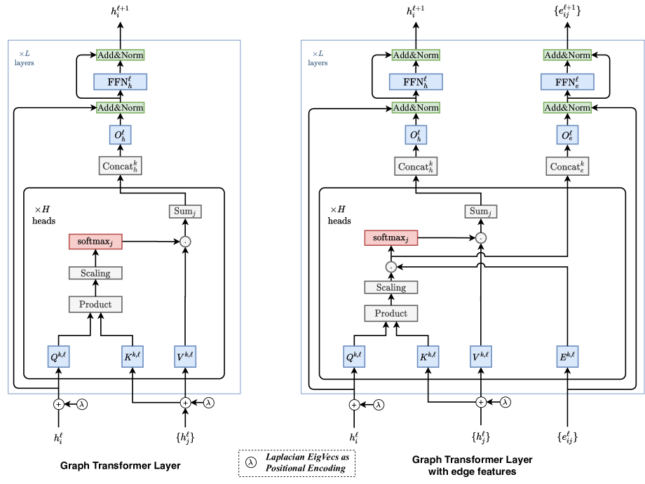
Figure 1: Block Diagram of Graph Transformer with Laplacian Eigvectors ($\lambda$) used as positional encoding (LapPE). LapPE is added to input node embeddings before passing the features to the first layer. Left: Graph Transformer operating on node embeddings only to compute attention scores; Right: Graph Transformer with edge features with designated feature pipeline to maintain layer wise edge representations. In this extension, the available edge attributes in a graph is used to explicitly modify the corresponding pairwise attention scores.

1.1 Related Work

As a preliminary, we highlight the most recent research works which attempt to develop graph transformers (Li et al. 2019; Nguyen, Nguyen, and Phung 2019; Zhang et al. 2020) with few focused on specialized cases such as on heterogeneous graphs, temporal networks, generative modeling, etc. (Yun et al. 2019; Xu, Joshi, and Bresson 2019; Hu et al. 2020; Zhou et al. 2020).

The model proposed in Li et al. (2019) employs attention to all graph nodes instead of a node’s local neighbors for the purpose of capturing global information. This limits the efficient exploitation of sparsity which we show is a good inductive bias for learning on graph datasets. For the purpose of global information, we argue that there are other ways to incorporate the same instead of letting go sparsity and local contexts. For example, the use of graph-specific positional features (Zhang et al. 2020), or node Laplacian position eigenvectors (Belkin and Niyogi 2003; Dwivedi et al. 2020), or relative learnable positional information (You, Ying, and Leskovec 2019), virtual nodes (Li et al. 2015), etc. Zhang et al. (2020) propose Graph-BERT with an emphasis on pre-training and parallelized learning using a subgraph batching scheme that creates fixed-size linkless subgraphs to be passed to the model instead of the original graph. Graph-BERT employs a combination of several positional encoding schemes to capture absolute node structural and relative node positional information. Since the original graph is not used directly in Graph-BERT and the subgraphs do not have edges between the nodes (i.e., linkless), the proposed combination of positional encodings attempts at retaining the original graph structure information in the nodes. We perform detailed analysis of Graph-BERT positional encoding schemes, along with experimental comparison with the model we present in this paper in Section 4.1.

Yun et al. (2019) developed Graph Transformer Networks (GTN) to learn on heterogeneous graphs with a target to transform a given heterogeneous graph into a meta-path based graph and then perform convolution. Notably, their focus behind the use of attention framework is for interpreting the generated meta-paths. There is another transformer based approach developed for heterogeneous information networks, namely Heterogeneous Graph Transformer (HGT) by Hu et al. (2020). Apart from its ability of handling arbitrary number of node and edge types, HGT also captures the dynamics of information flow in the heterogeneous graphs in the form of relative temporal positional encoding which is based on the timestamp differences of the central node and the message-passing nodes. Furthermore, Zhou et al. (2020) proposed a transformer based generative model which generates temporal graphs by directly learning from dynamic information in networks. The architecture presented in Nguyen, Nguyen, and Phung (2019) somewhat proceeds along our goal to develop graph transformer for arbitrary homogeneous graphs with a coordinate embedding based positional encoding scheme. However, their experiments show that the coordinate embeddings are not universal in performance and only helps in a couple of unsupervised learning experiments among all evaluations.

1.2 Contributions

Overall, we find that the most fruitful ideas from the transformers literature in NLP can be applied in a more efficient way and posit that sparsity and positional encodings are two key aspects in the development of a Graph Transformer. As opposed to designing a best performing model for specific graph tasks, our work attempts for a generic, competitive transformer model which draws ideas together from the domains of NLP and GNNs. For an overview, this paper brings the following contributions:

• We put forward a generalization of transformer networks to homogeneous graphs of arbitrary structure, namely Graph Transformer, and an extended version of Graph Transformer with edge features that allows the usage of explicit domain information as edge features.

• Our method includes an elegant way to fuse node positional features using Laplacian eigenvectors for graph datasets, inspired from the heavy usage of positional encodings in NLP transformer models and recent research on node positional features in GNNs. The comparison with literature shows Laplacian eigenvectors to be well-placed than any existing approaches to encode node positional information for arbitrary homogeneous graphs.

• Our experiments demonstrate that the proposed model surpasses baseline isotropic and anisotropic GNNs. The architecture simultaneously emerges as a better attention based GNN baseline as well as a simple and effective Transformer network baseline for graph datasets for future research at the intersection of attention and graphs.

2 Proposed Architecture

As stated earlier, we take into account two key aspects to develop Graph Transformers – sparsity and positional encodings which should ideally be used in the best possible way for learning on graph datasets. We first discuss the motivations behind these using a transition from NLP to graphs, and then introduce the architecture proposed.

2.1 On Graph Sparsity

In NLP transformers, a sentence is treated as a fully connected graph and this choice can be justified for two reasons – a) First, it is difficult to find meaningful sparse interactions or connections among the words in a sentence. For instance, the dependency of a word in a sentence on another word can vary with context, perspective of a user and specific application. There can be numerous plausible ground truth connections among words in a sentence and therefore, text datasets of sentences do not have explicit word interactions available. It thereby makes sense to have each word attending to each other word in a sentence, as followed by the Transformer architecture (Vaswani et al. 2017). – b) Next, the so-called graph considered in an NLP transformer often has less than tens or hundreds of nodes (i.e. sentences are often less than tens or hundreds of words). This makes for computationally feasibility and large transformer models can be trained on such fully connected graphs of words.

In case of actual graph datasets, graphs have arbitrary connectivity structure available depending on the domain and target of application, and have node sizes in ranges of up to millions, or billions. The available structure presents us with a rich source of information to exploit as an inductive bias in a neural network, whereas the node sizes practically makes it impossible to have a fully connected graph for such datasets. On these accounts, it is ideal and practical to have a Graph Transformer where a node attends to local node neighbors, same as in GNNs (Defferrard, Bresson, and Vandergheynst 2016; Kipf and Welling 2017; Monti et al. 2017; Gilmer et al. 2017; Veličković et al. 2018; Bresson and Laurent 2017; Xu et al. 2019).

2.2 On Positional Encodings

In NLP, transformer based models are, in most cases, supplied with a positional encoding for each word. This is critical to ensure unique representation for each word, and eventually preserve distance information. For graphs, the design of unique node positions is challenging as there are symmetries which prevent canonical node positional information (Murphy et al. 2019). In fact, most of the GNNs which are trained on graph datasets learn structural node information that are invariant to the node position (Srinivasan and Ribeiro 2020). This is a critical reason why simple attention based models, such as GAT (Veličković et al. 2018), where the attention is a function of local neighborhood connectivity, instead full-graph connectivity, do not seem to achieve competitive performance on graph datasets. The issue of positional embeddings has been explored in recent GNN works (Murphy et al. 2019; You, Ying, and Leskovec 2019; Srinivasan and Ribeiro 2020; Dwivedi et al. 2020; Li et al. 2020) with a goal to learn both structural and positional features. In particular, Dwivedi et al. (2020) make the use of available graph structure to pre-compute Laplacian eigenvectors (Belkin and Niyogi 2003) and use them as node positional information. Since Laplacian PEs are generalization of the PE used in the original transformers (Vaswani et al. 2017) to graphs and these better help encode distance-aware information (i.e., nearby nodes have similar positional features and farther nodes have dissimilar positional features), we use Laplacian eigenvectors as PE in Graph Transformer. Although these eigenvectors have multiplicity occuring due to the arbitrary sign of eigenvectors, we randomly flip the sign of the eigenvectors during training, following Dwivedi et al. (2020).We pre-compute the Laplacian eigenvectors of all graphs in the dataset. Eigenvectors are defined via the factorization of the graph Laplacian matrix;

$$\Delta=\textrm{I}-D^{-1/2}AD^{-1/2}=U^{T}\Lambda U,$$ (1)

where $A$ is the $n\times n$ adjacency matrix, $D$ is the degree matrix, and $\Lambda$, $U$ correspond to the eigenvalues and eigenvectors respectively. We use the $k$ smallest non-trivial eigenvectors of a node as its positional encoding and denote by ${\lambda}_{i}$ for node $i$. Finally, we refer to Section 4.1 for a comparison of Laplacian PE with existing Graph-BERT PEs.

2.3 Graph Transformer Architecture

We now introduce the Graph Transformer Layer and Graph Transformer Layer with edge features. The layer architecture is illustrated in Figure 1. The first model is designed for graphs which do not have explicit edge attributes, whereas the second model maintains a designated edge feature pipeline to incorporate the available edge information and maintain their abstract representations at every layer.

Input

First of all, we prepare the input node and edge embeddings to be passed to the Graph Transformer Layer. For a graph $\mathcal{G}$ with node features $\alpha_{i}\in\mathbb{R}^{d_{n}\times 1}$ for each node $i$ and edge features $\beta_{ij}\in\mathbb{R}^{d_{e}\times 1}$ for each edge between node $i$ and node $j$, the input node features $\alpha_{i}$ and edge features $\beta_{ij}$ are passed via a linear projection to embed these to $d$-dimensional hidden features $h_{i}^{0}$ and $e_{ij}^{0}$.

$$\hat{h}_{i}^{0}=A^{0}\alpha_{i}+a^{0}\;\ ;\;\ e_{ij}^{0}=B^{0}\beta_{ij}+b^{0},$$ (2)

where $A^{0}\in\mathbb{R}^{d\times d_{n}}$, $B^{0}\in\mathbb{R}^{d\times d_{e}}$ and $a^{0},b^{0}\in\mathbb{R}^{d}$ are the parameters of the linear projection layers. We now embed the pre-computed node positional encodings of dim $k$ via a linear projection and add to the node features $\hat{h}_{i}^{0}$.

$${\lambda}_{i}^{0}=C^{0}\lambda_{i}+c^{0}\;\ ;\;\ h_{i}^{0}=\hat{h}_{i}^{0}+{\lambda}_{i}^{0},$$ (3)

where $C^{0}\in\mathbb{R}^{d\times k}$ and $c^{0}\in\mathbb{R}^{d}$. Note that the Laplacian positional encodings are only added to the node features at the input layer and not during intermediate Graph Transformer layers.

Graph Transformer Layer

The Graph Transformer is closely the same transformer architecture initially proposed in (Vaswani et al. 2017), see Figure 1 (Left). We now proceed to define the node update equations for a layer $\ell$.

$$\hat{h}_{i}^{\ell+1}=O_{h}^{\ell}\ \bigparallel_{k=1}^{H}\Big{(}\sum_{j\in\mathcal{N}_{i}}w_{ij}^{k,\ell}V^{k,\ell}h_{j}^{\ell}\Big{)},$$ (4)

$$\textnormal{where,}\ w_{ij}^{k,\ell}=\textnormal{softmax}_{j}\Big{(}\frac{Q^{k,\ell}h_{i}^{\ell}\ \cdot\ K^{k,\ell}h_{j}^{\ell}}{\sqrt{d_{k}}}\Big{)},$$ (5)

and $Q^{k,\ell},K^{k,\ell},V^{k,\ell}\in\mathbb{R}^{d_{k}\times d}$, $O_{h}^{\ell}\in\mathbb{R}^{d\times d}$, $k=1$ to $H$ denotes the number of attention heads, and $\|$ denotes concatenation. For numerical stability, the outputs after taking exponents of the terms inside softmax is clamped to a value between $-5$ to $+5$. The attention outputs $\hat{h}_{i}^{\ell+1}$ are then passed to a Feed Forward Network (FFN) preceded and succeeded by residual connections and normalization layers, as:

$$\hat{\hat{h}}_{i}^{\ell+1} = \textnormal{Norm}\Big{(}h_{i}^{\ell}+\hat{h}_{i}^{\ell+1}\Big{)},$$ (6)

$$\hat{\hat{\hat{h}}}_{i}^{\ell+1} = W_{2}^{\ell}\textnormal{ReLU}(W_{1}^{\ell}\hat{\hat{h}}_{i}^{\ell+1}),$$ (7)

$$h_{i}^{\ell+1} = \textnormal{Norm}\Big{(}\hat{\hat{h}}_{i}^{\ell+1}+\hat{\hat{\hat{h}}}_{i}^{\ell+1}\Big{)},$$ (8)

where $W_{1}^{\ell},\in\mathbb{R}^{2d\times d}$, $W_{2}^{\ell},\in\mathbb{R}^{d\times 2d}$, $\hat{\hat{h}}_{i}^{\ell+1},\hat{\hat{\hat{h}}}_{i}^{\ell+1}$ denote intermediate representations, and Norm can either be LayerNorm(Ba, Kiros, and Hinton 2016) or BatchNorm (Ioffe and Szegedy 2015). The bias terms are omitted for clarity of presentation.

Graph Transformer Layer with edge features

The Graph Transformer with edge features is designed for better utilization of rich feature information available in several graph datasets in the form of edge attributes. See Figure 1 (Right) for a reference to the building block of a layer. Since our objective remains to better use the edge features which are pairwise scores corresponding to a node pair, we tie these available edge features to implicit edge scores computed by pairwise attention. In other words, say an intermediate attention score before softmax, $\hat{w}_{ij}$, is computed when a node $i$ attends to node $j$ after the multiplication of query and key feature projections, see the expression inside the brackets in Equation 5. Let us treat this score $\hat{w}_{ij}$ as implicit information about the edge $<i,j>$. We now try to inject the available edge information for the edge $<i,j>$ and improve the already computed implicit attention score $\hat{w}_{ij}$. It is done by simply multiplying the two values $\hat{w}_{ij}$ and $e_{ij}$, see Equation 12. This kind of information injection is not seen to be explored much, or applied in NLP Transformers as there is usually no available feature information between two words. However, in graph datasets such as molecular graphs, or social media graphs, there is often some feature information available on the edge interactions and it becomes natural to design an architecture to use this information while learning. For the edges, we also maintain a designated node-symmetric edge feature representation pipeline for propagating edge attributes from one layer to another, see Figure 1. We now proceed to define the layer update equations for a layer $\ell$.

$$\hat{h}_{i}^{\ell+1} = O_{h}^{\ell}\ \bigparallel_{k=1}^{H}\Big{(}\sum_{j\in\mathcal{N}_{i}}w_{ij}^{k,\ell}V^{k,\ell}h_{j}^{\ell}\Big{)},$$ (9)

$$\hat{e}_{ij}^{\ell+1} = O_{e}^{\ell}\ \bigparallel_{k=1}^{H}\Big{(}\hat{w}_{ij}^{k,\ell}\Big{)},\ \ \textnormal{where,}$$ (10)

$$w_{ij}^{k,\ell} = \textnormal{softmax}_{j}(\hat{w}_{ij}^{k,\ell}),$$ (11)

$$\hat{w}_{ij}^{k,\ell} = \Big{(}\frac{Q^{k,\ell}h_{i}^{\ell}\ \cdot\ K^{k,\ell}h_{j}^{\ell}}{\sqrt{d_{k}}}\Big{)}\ \cdot\ E^{k,\ell}e^{\ell}_{ij},$$ (12)

and $Q^{k,\ell},K^{k,\ell},V^{k,\ell},E^{k,\ell}\in\mathbb{R}^{d_{k}\times d}$, $O_{h}^{\ell},O_{e}^{\ell}\in\mathbb{R}^{d\times d}$, $k=1$ to $H$ denotes the number of attention head, and $\|$ denotes concatenation. For numerical stability, the outputs after taking exponents of the terms inside softmax is clamped to a value between $-5$ to $+5$. The outputs $\hat{h}_{i}^{\ell+1}$ and $\hat{e}_{ij}^{\ell+1}$ are then passed to separate Feed Forward Networks preceded and succeeded by residual connections and normalization layers, as:

$$\hat{\hat{h}}_{i}^{\ell+1} = \textnormal{Norm}\Big{(}h_{i}^{\ell}+\hat{h}_{i}^{\ell+1}\Big{)},$$ (13)

$$\hat{\hat{\hat{h}}}_{i}^{\ell+1} = W_{h,2}^{\ell}\textnormal{ReLU}(W_{h,1}^{\ell}\hat{\hat{h}}_{i}^{\ell+1}),$$ (14)

$$h_{i}^{\ell+1} = \textnormal{Norm}\Big{(}\hat{\hat{h}}_{i}^{\ell+1}+\hat{\hat{\hat{h}}}_{i}^{\ell+1}\Big{)},$$ (15)

where $W_{h,1}^{\ell},\in\mathbb{R}^{2d\times d}$, $W_{h,2}^{\ell},\in\mathbb{R}^{d\times 2d}$, $\hat{\hat{h}}_{i}^{\ell+1},\hat{\hat{\hat{h}}}_{i}^{\ell+1}$ denote intermediate representations,

$$\hat{\hat{e}}_{ij}^{\ell+1} = \textnormal{Norm}\Big{(}e_{ij}^{\ell}+\hat{e}_{ij}^{\ell+1}\Big{)},$$ (16)

$$\hat{\hat{\hat{e}}}_{ij}^{\ell+1} = W_{e,2}^{\ell}\textnormal{ReLU}(W_{e,1}^{\ell}\hat{\hat{e}}_{ij}^{\ell+1}),$$ (17)

$$e_{ij}^{\ell+1} = \textnormal{Norm}\Big{(}\hat{\hat{e}}_{ij}^{\ell+1}+\hat{\hat{\hat{e}}}_{ij}^{\ell+1}\Big{)},$$ (18)

where $W_{e,1}^{\ell},\in\mathbb{R}^{2d\times d}$, $W_{e,2}^{\ell},\in\mathbb{R}^{d\times 2d}$, $\hat{\hat{e}}_{ij}^{\ell+1},\hat{\hat{\hat{e}}}_{ij}^{\ell+1}$ denote intermediate representations.

Task based MLP Layers

The node representations obtained at the final layer of Graph Transformer are passed to a task based MLP network for computing task-dependent outputs, which are then fed to a loss function to train the parameters of the model. The formal definitions of the task based layers that we use can be found in Appendix A.1.

3 Numerical Experiments

				Sparse Graph				Full Graph
Dataset	LapPE	$L$	#Param	Test Perf.$\pm$s.d.	Train Perf.$\pm$s.d.	#Epoch	Epoch/Total	Test Perf.$\pm$s.d.	Train Perf.$\pm$s.d.	#Epoch	Epoch/Total
Batch Norm: False; Layer Norm: True
ZINC	x	10	588353	0.278$\pm$0.018	0.027$\pm$0.004	274.75	26.87s/2.06hr	0.741$\pm$0.008	0.431$\pm$0.013	196.75	37.64s/2.09hr
	✓	10	588929	0.284$\pm$0.012	0.031$\pm$0.006	263.00	26.64s/1.98hr	0.735$\pm$0.006	0.442$\pm$0.031	196.75	31.50s/1.77hr
CLUSTER	x	10	523146	70.879$\pm$0.295	86.174$\pm$0.365	128.50	202.68s/7.32hr	19.596$\pm$2.071	19.570$\pm$2.053	103.00	512.34s/15.15hr
	✓	10	524026	70.649$\pm$0.250	86.395$\pm$0.528	130.75	200.55s/7.43hr	27.091$\pm$3.920	26.916$\pm$3.764	139.50	565.13s/22.37hr
PATTERN	x	10	522742	73.140$\pm$13.633	73.070$\pm$13.589	184.25	276.66s/13.75hr	50.854$\pm$0.111	50.906$\pm$0.005	108.00	540.85s/16.77hr
	✓	10	522982	71.005$\pm$11.831	71.125$\pm$11.977	192.50	294.91s/14.79hr	56.482$\pm$3.549	56.565$\pm$3.546	124.50	637.55s/22.69hr
Batch Norm: True; Layer Norm: False
ZINC	x	10	588353	0.264$\pm$0.008	0.048$\pm$0.006	321.50	28.01s/2.52hr	0.724$\pm$0.013	0.518$\pm$0.013	192.25	50.27s/2.72hr
	✓	10	588929	0.226$\pm$0.014	0.059$\pm$0.011	287.50	27.78s/2.25hr	0.598$\pm$0.049	0.339$\pm$0.123	273.50	45.26s/3.50hr
CLUSTER	x	10	523146	72.139$\pm$0.405	85.857$\pm$0.555	121.75	200.85s/6.88hr	21.092$\pm$0.134	21.071$\pm$0.037	100.25	595.24s/17.10hr
	✓	10	524026	73.169$\pm$0.622	86.585$\pm$0.905	126.50	201.06s/7.20hr	27.121$\pm$8.471	27.192$\pm$8.485	133.75	552.06s/20.72hr
PATTERN	x	10	522742	83.949$\pm$0.303	83.864$\pm$0.489	236.50	299.54s/19.71hr	50.889$\pm$0.069	50.873$\pm$0.039	104.50	621.33s/17.53hr
	✓	10	522982	84.808$\pm$0.068	86.559$\pm$0.116	145.25	309.95s/12.67hr	54.941$\pm$3.739	54.915$\pm$3.769	117.75	683.53s/22.77hr

Table 1: Results of GraphTransformer (GT) on all datasets. Performance Measure for ZINC is MAE, for PATTERN and CLUSTER is Acc. Results (higher is better for all except ZINC) are averaged over 4 runs with 4 different seeds. Bold: the best performing model for each dataset. We perform each experiment with given graphs (Sparse Graph) and (Full Graph) in which we create full connections among all nodes; For ZINC full graphs, edge features are discarded given our motive of the full graph experiments without any sparse structure information.

Model	ZINC	CLUSTER	PATTERN
GNN BASELINE SCORES from (Dwivedi et al. 2020)
GCN	0.367$\pm$0.011	68.498$\pm$0.976	71.892$\pm$0.334
GAT	0.384$\pm$0.007	70.587$\pm$0.447	78.271$\pm$0.186
GatedGCN	0.214$\pm$0.013	76.082$\pm$0.196	86.508$\pm$0.085
OUR RESULTS
GT (Ours)	0.226$\pm$0.014	73.169$\pm$0.622	84.808$\pm$0.068

Table 2: Comparison of our best performing scores (from Table 1) on each dataset against the GNN baselines (GCN (Kipf and Welling 2017), GAT (Veličković et al. 2018), GatedGCN(Bresson and Laurent 2017)) of 500k model parameters. Note: Only GatedGCN and GT models use the available edge attributes in ZINC.

We evaluate the performance of proposed Graph Transformer on three benchmark graph datasets– ZINC (Irwin et al. 2012), PATTERN and CLUSTER (Abbe 2017) from a recent GNN benchmark (Dwivedi et al. 2020).

ZINC, Graph Regression

ZINC (Irwin et al. 2012) is a molecular dataset with the task of graph property regression for constrained solubility. Each ZINC molecule is represented as a graph of atoms as nodes and bonds as edges. Since this dataset have rich feature information in terms of bonds as edge attributes, we use the ‘Graph Transformer with edge features’ for this task. We use the 12K subset of the data as in Dwivedi et al. (2020).

PATTERN, Node Classification

PATTERN is a node classification dataset generated using the Stochastic Block Models (SBM) (Abbe 2017). The task is classify the nodes into 2 communities. PATTERN graphs do not have explicit edge features and hence we use the simple ‘Graph Transformer’ for this task. The size of this dataset is 14K graphs.

CLUSTER, Node Classification

CLUSTER is also a synthetically generated dataset using SBM model. The task is to assign a cluster label to each node. There are total 6 cluster labels. Similar to PATTERN, CLUSTER graphs do not have explicit edge features and hence we use the simple ‘Graph Transformer’ for this task. The size of this dataset is 12K graphs. We refer the readers to (Dwivedi et al. 2020) for additional information, inlcuding preparation, of these datasets.

Model Configurations

For experiments, we follow the benchmarking protocol introduced in Dwivedi et al. (2020) based on PyTorch (Paszke et al. 2019) and DGL (Wang et al. 2019). We use 10 layers of Graph Transformer layers with each layer having 8 attention heads and arbitrary hidden dimensions such that the total number of trainable parameters is in the range of 500k. We use learning rate decay strategy to train the models where the training stops at a point when the learning rate reaches to a value of $1\times 10^{-6}$. We run each experiment with 4 different seeds and report the mean and average performance measure of the 4 runs. The results are reported in Table 1 and comparison in Table 2.

4 Analysis and Discussion

We now present the analysis of our experiments on the proposed Graph Transformer Architecture, see Tables 1 and 2.

• The generalization of transformer network on graphs is best when Laplacian PE are used for node positions and Batch Normalization is selected instead of Layer Normalization. For all three benchmark datasets, the experiments score the highest performance in this setting, see Table 1.

• The proposed architecture performs significantly better than baseline isotropic and anisotropic GNNs (GCN and GAT respectively), and helps close the gap between the original transformer and transformer for graphs. Notably, our architecture emerges as a fresh and improved attention based GNN baseline surpassing GAT (see Table 2), which employs multi-headed attention inspired by the original transformer (Vaswani et al. 2017) and have been often used in the literature as a baseline for attention-based GNN models.

• As expected, sparse graph connectivity is a critical inductive bias for datasets with arbitrary graph structure, as demonstrated by comparing sparse vs. full graph experiments.

• Our proposed extension of Graph Transformer with edge features reaches close to the best performing GNN, i.e., GatedGCN, on ZINC. This architecture specifically brings exciting promise to datasets where domain information along pairwise interactions can be leveraged for maximum learning performance.

4.1 Comparison to PEs used in Graph-BERT

In addition to the reasons underscored in Sections 1.1 and 2.2, we demonstrate the usefulness of Laplacian eigenvectors as a suitable candidate PE for Graph Transformer in this section, by its comparison with different PE schemes applied in Graph-BERT (Zhang et al. 2020). In Graph-BERT, which operates on fixed size sampled subgraphs, a node attends to every other node in a subgraph. For a given graph $\mathcal{G}=(\mathcal{V},\mathcal{E})$ with $\mathcal{V}$ nodes and $\mathcal{E}$ edges, a subgraph $g_{i}$ of size $k+1$ is created for every node $i$ in the graph, which means the original single graph $\mathcal{G}$ is converted to $\mathcal{V}$ subgraphs. For a subgraph $g_{i}$ corresponding to node $u_{i}$, the $k$ other nodes are the ones which have the top $k$ intimacy scores with node $u_{i}$ based on a pre-computed intimacy matrix that maps every edge in the graph $\mathcal{G}$ to an intimacy score. While the sampling is great for parallelization and efficiency, the original graph structure is not directly used in the layers. Graph-BERT uses a combination of node PE schemes to inform the model on node structural, positional, and distance information from original graph– i) Intimacy based relative PE, ii) Hop based relative distance encoding, and iii) Weisfeiler Lehman based absolute PE (WL-PE). The intimacy based PE and the hop based PE are variant to the sampled subgraphs, i.e., these PEs for a node in a subgraph $g_{i}$ depends on the node $u_{i}$ w.r.t which it is sampled, and cannot be directly used in other cases unless we use similar sampling strategy. The WL-PE which are absolute structural roles of nodes in the original graph computed using WL algorithm (Zhang et al. 2020; Niepert, Ahmed, and Kutzkov 2016), are not variant to the subgraphs and can be easily used as a generic PE mechanism. On that account, we swap Laplacian PE in our experiments for an ablation analysis and use WL-PE from Graph-BERT, see Table 3. As Laplacian PE capture better structural and positional information about the nodes, which essentially is the objective behind using the three Graph-BERT PEs, they outperform the WL-PE. Besides, WL-PEs tend to overfit SBM datasets and lead to poor generalization.

			Sparse Graph
Dataset	PE	#Param	Test Perf.$\pm$s.d.	Train Perf.$\pm$s.d.	#Epoch	Epoch/Total
Batch Norm: True; Layer Norm: False; $L$ = 10
ZINC	x	588353	0.264$\pm$0.008	0.048$\pm$0.006	321.50	28.01s/2.52hr
	L	588929	0.226$\pm$0.014	0.059$\pm$0.011	287.50	27.78s/2.25hr
	W	590721	0.267$\pm$0.012	0.059$\pm$0.010	263.25	27.04s/2.00hr
CLUSTER	x	523146	72.139$\pm$0.405	85.857$\pm$0.555	121.75	200.85s/6.88hr
	L	524026	73.169$\pm$0.622	86.585$\pm$0.905	126.50	201.06s/7.20hr
	W	531146	70.790$\pm$0.537	86.829$\pm$0.745	119.00	196.41s/6.69hr
PATTERN	x	522742	83.949$\pm$0.303	83.864$\pm$0.489	236.50	299.54s/19.71hr
	L	522982	84.808$\pm$0.068	86.559$\pm$0.116	145.25	309.95s/12.67hr
	W	530742	75.489$\pm$0.216	97.028$\pm$0.104	109.25	310.11s/9.73hr

Table 3: Analysis of GraphTransformer (GT) using different PE schemes. Notations x: No PE; L: LapPE (ours); W: WL-PE (Zhang et al. 2020). Bold: the best performing model for each dataset.

5 Conclusion

This work presented a simple yet effective approach to generalize transformer networks on arbitrary graphs and introduced the corresponding architecture. Our experiments consistently showed that the presence of – i) Laplacian eigenvectors as node positional encodings and – ii) batch normalization, in place of layer normalization, around the transformer feed forward layers enhanced the transformer universally on all experiments. Given the simple and generic nature of our architecture and competitive performance against standard GNNs, we believe the proposed model can be used as baseline for further improvement across graph applications employing node attention. In future works, we are interested in building upon the graph transformer along aspects such as efficient training on single large graphs, applicability on heterogeneous domains, etc., and perform efficient graph representation learning keeping in account the recent innovations in graph inductive biases.

Appendix A Appendix

A.1 Task based MLP layer equations

Graph prediction layer

For graph prediction task, the final layer node features of a graph is averaged to get a $d$-dimensional graph-level feature vector $y_{\mathcal{G}}$.

$$y_{\mathcal{G}}=\frac{1}{\mathcal{V}}\sum_{i=0}^{\mathcal{V}}{h_{i}^{L}},$$ (19)

The graph feature vector is then passed to a MLP to obtain the un-normalized prediction score for each class, $y_{\textnormal{pred}}\in\mathbb{R}^{C}$ for each class:

$$y_{\textnormal{pred}}=P\ \textnormal{ReLU}\left(Q\ y_{\mathcal{G}}\right),$$ (20)

where $P\in\mathbb{R}^{d\times C},Q\in\mathbb{R}^{d\times d},C$ is the number of task labels (classes) to be predicted. Since we perform single-target graph regression in ZINC, $C=1$, and the L1-loss between the predicted and groundtruth values is minimized during training.

Node prediction layer

For node prediction task, each node’s feature vector is passed to a MLP for computing the un-normalized prediction scores $y_{i,\textnormal{pred}}\in\mathbb{R}^{C}$ for each class:

$$y_{i,\textnormal{pred}}=P\ \textnormal{ReLU}\left(Q\ h_{i}^{L}\right),$$ (21)

where $P\in\mathbb{R}^{d\times C},Q\in\mathbb{R}^{d\times d}$. During training, the cross-entropy loss weighted inversely by the class size is used.

As a note, these task based layers can be modified as per the requirements of the dataset, and or the prediction to be done. For example, the Graph Transformer edge outputs (Figure 1 (Right)) can be used for edge prediction tasks and the task based MLP layers can be defined in similar fashion as we do for node prediction. Besides, different styles of using final and/or intermediate Graph Transformer layers can be used as inputs to the task based MLP layers, such as JK Readout (Jumping Knowledge) (Xu et al. 2018), etc. used often in GNNs.

A.2 Hardware Information

All experiments are run on Intel Xeon CPU E5-2690 v4 server with 4 Nvidia 1080Ti GPUs. At a given time, 4 experiments were run on the server with each single GPU running 1 experiment. The maximum training time for an experiment is limited to 24 hours.

References

- Abbe (2017) Abbe, E. 2017. Community detection and stochastic block models: recent developments. The Journal of Machine Learning Research 18(1): 6446–6531.
- Ba, Kiros, and Hinton (2016) Ba, J. L.; Kiros, J. R.; and Hinton, G. E. 2016. Layer normalization. NeurIPS workshop on Deep Learning .
- Bahdanau, Cho, and Bengio (2014) Bahdanau, D.; Cho, K.; and Bengio, Y. 2014. Neural machine translation by jointly learning to align and translate. arXiv preprint arXiv:1409.0473 .
- Belkin and Niyogi (2003) Belkin, M.; and Niyogi, P. 2003. Laplacian eigenmaps for dimensionality reduction and data representation. Neural computation 15(6): 1373–1396.
- Bresson and Laurent (2017) Bresson, X.; and Laurent, T. 2017. Residual gated graph convnets. arXiv preprint arXiv:1711.07553 .
- Brown et al. (2020) Brown, T. B.; Mann, B.; Ryder, N.; Subbiah, M.; Kaplan, J.; Dhariwal, P.; Neelakantan, A.; Shyam, P.; Sastry, G.; Askell, A.; et al. 2020. Language models are few-shot learners. arXiv preprint arXiv:2005.14165 .
- Chami et al. (2020) Chami, I.; Wolf, A.; Juan, D.-C.; Sala, F.; Ravi, S.; and Ré, C. 2020. Low-Dimensional Hyperbolic Knowledge Graph Embeddings. arXiv preprint arXiv:2005.00545 .
- Cranmer et al. (2019) Cranmer, M. D.; Xu, R.; Battaglia, P.; and Ho, S. 2019. Learning Symbolic Physics with Graph Networks. arXiv preprint arXiv:1909.05862 .
- Defferrard, Bresson, and Vandergheynst (2016) Defferrard, M.; Bresson, X.; and Vandergheynst, P. 2016. Convolutional Neural Networks on Graphs with Fast Localized Spectral Filtering. In Advances in Neural Information Processing Systems 29, 3844–3852.
- Devlin et al. (2018) Devlin, J.; Chang, M.-W.; Lee, K.; and Toutanova, K. 2018. Bert: Pre-training of deep bidirectional transformers for language understanding. arXiv preprint arXiv:1810.04805 .
- Dwivedi et al. (2020) Dwivedi, V. P.; Joshi, C. K.; Laurent, T.; Bengio, Y.; and Bresson, X. 2020. Benchmarking graph neural networks. arXiv preprint arXiv:2003.00982 .
- Gilmer et al. (2017) Gilmer, J.; Schoenholz, S. S.; Riley, P. F.; Vinyals, O.; and Dahl, G. E. 2017. Neural message passing for quantum chemistry. In Proceedings of the 34th International Conference on Machine Learning-Volume 70, 1263–1272. JMLR. org.
- Hu et al. (2020) Hu, Z.; Dong, Y.; Wang, K.; and Sun, Y. 2020. Heterogeneous graph transformer. In Proceedings of The Web Conference 2020, 2704–2710.
- Ioffe and Szegedy (2015) Ioffe, S.; and Szegedy, C. 2015. Batch normalization: Accelerating deep network training by reducing internal covariate shift. arXiv preprint arXiv:1502.03167 .
- Irwin et al. (2012) Irwin, J. J.; Sterling, T.; Mysinger, M. M.; Bolstad, E. S.; and Coleman, R. G. 2012. ZINC: a free tool to discover chemistry for biology. Journal of chemical information and modeling 52(7): 1757–1768.
- Joshi (2020) Joshi, C. 2020. Transformers are Graph Neural Networks. The Gradient .
- Kipf and Welling (2017) Kipf, T. N.; and Welling, M. 2017. Semi-Supervised Classification with Graph Convolutional Networks. In International Conference on Learning Representations (ICLR).
- Li et al. (2020) Li, P.; Wang, Y.; Wang, H.; and Leskovec, J. 2020. Distance Encoding–Design Provably More Powerful GNNs for Structural Representation Learning. arXiv preprint arXiv:2009.00142 .
- Li et al. (2019) Li, Y.; Liang, X.; Hu, Z.; Chen, Y.; and Xing, E. P. 2019. Graph Transformer. URL https://openreview.net/forum?id=HJei-2RcK7.
- Li et al. (2015) Li, Y.; Tarlow, D.; Brockschmidt, M.; and Zemel, R. 2015. Gated graph sequence neural networks. arXiv preprint arXiv:1511.05493 .
- Monti et al. (2017) Monti, F.; Boscaini, D.; Masci, J.; Rodola, E.; Svoboda, J.; and Bronstein, M. M. 2017. Geometric Deep Learning on Graphs and Manifolds Using Mixture Model CNNs. 2017 IEEE Conference on Computer Vision and Pattern Recognition (CVPR) doi:10.1109/cvpr.2017.576.
- Monti et al. (2019) Monti, F.; Frasca, F.; Eynard, D.; Mannion, D.; and Bronstein, M. M. 2019. Fake news detection on social media using geometric deep learning. arXiv preprint arXiv:1902.06673 .
- Murphy et al. (2019) Murphy, R.; Srinivasan, B.; Rao, V.; and Ribeiro, B. 2019. Relational Pooling for Graph Representations. In International Conference on Machine Learning, 4663–4673.
- Nguyen, Nguyen, and Phung (2019) Nguyen, D. Q.; Nguyen, T. D.; and Phung, D. 2019. Universal Self-Attention Network for Graph Classification. arXiv preprint arXiv:1909.11855 .
- Niepert, Ahmed, and Kutzkov (2016) Niepert, M.; Ahmed, M.; and Kutzkov, K. 2016. Learning convolutional neural networks for graphs. In International conference on machine learning, 2014–2023.
- Paszke et al. (2019) Paszke, A.; Gross, S.; Massa, F.; Lerer, A.; Bradbury, J.; Chanan, G.; Killeen, T.; Lin, Z.; Gimelshein, N.; Antiga, L.; Desmaison, A.; Köpf, A.; Yang, E.; DeVito, Z.; Raison, M.; Tejani, A.; Chilamkurthy, S.; Steiner, B.; Fang, L.; Bai, J.; and Chintala, S. 2019. PyTorch: An Imperative Style, High-Performance Deep Learning Library.
- Radford et al. (2018) Radford, A.; Narasimhan, K.; Salimans, T.; and Sutskever, I. 2018. Improving language understanding by generative pre-training.
- Sanchez-Gonzalez et al. (2020) Sanchez-Gonzalez, A.; Godwin, J.; Pfaff, T.; Ying, R.; Leskovec, J.; and Battaglia, P. W. 2020. Learning to simulate complex physics with graph networks. arXiv preprint arXiv:2002.09405 .
- Schlichtkrull et al. (2018) Schlichtkrull, M.; Kipf, T. N.; Bloem, P.; Van Den Berg, R.; Titov, I.; and Welling, M. 2018. Modeling relational data with graph convolutional networks. In European Semantic Web Conference, 593–607. Springer.
- Srinivasan and Ribeiro (2020) Srinivasan, B.; and Ribeiro, B. 2020. On the Equivalence between Node Embeddings and Structural Graph Representations. International Conference on Learning Representations .
- Vaswani et al. (2017) Vaswani, A.; Shazeer, N.; Parmar, N.; Uszkoreit, J.; Jones, L.; Gomez, A. N.; Kaiser, Ł.; and Polosukhin, I. 2017. Attention is all you need. In Advances in neural information processing systems, 5998–6008.
- Veličković et al. (2018) Veličković, P.; Cucurull, G.; Casanova, A.; Romero, A.; Liò, P.; and Bengio, Y. 2018. Graph Attention Networks. International Conference on Learning Representations .
- Wang et al. (2019) Wang, M.; Yu, L.; Zheng, D.; Gan, Q.; Gai, Y.; Ye, Z.; Li, M.; Zhou, J.; Huang, Q.; Ma, C.; Huang, Z.; Guo, Q.; Zhang, H.; Lin, H.; Zhao, J.; Li, J.; Smola, A. J.; and Zhang, Z. 2019. Deep Graph Library: Towards Efficient and Scalable Deep Learning on Graphs. ICLR Workshop on Representation Learning on Graphs and Manifolds .
- Xu et al. (2019) Xu, K.; Hu, W.; Leskovec, J.; and Jegelka, S. 2019. How Powerful are Graph Neural Networks? In International Conference on Learning Representations.
- Xu et al. (2018) Xu, K.; Li, C.; Tian, Y.; Sonobe, T.; Kawarabayashi, K.-i.; and Jegelka, S. 2018. Representation learning on graphs with jumping knowledge networks. arXiv preprint arXiv:1806.03536 .
- Xu, Joshi, and Bresson (2019) Xu, P.; Joshi, C. K.; and Bresson, X. 2019. Multi-graph transformer for free-hand sketch recognition. arXiv preprint arXiv:1912.11258 .
- You, Ying, and Leskovec (2019) You, J.; Ying, R.; and Leskovec, J. 2019. Position-aware graph neural networks. International Conference on Machine Learning .
- Yun et al. (2019) Yun, S.; Jeong, M.; Kim, R.; Kang, J.; and Kim, H. J. 2019. Graph transformer networks. In Advances in Neural Information Processing Systems, 11983–11993.
- Zhang et al. (2020) Zhang, J.; Zhang, H.; Sun, L.; and Xia, C. 2020. Graph-Bert: Only Attention is Needed for Learning Graph Representations. arXiv preprint arXiv:2001.05140 .
- Zhou et al. (2020) Zhou, D.; Zheng, L.; Han, J.; and He, J. 2020. A Data-Driven Graph Generative Model for Temporal Interaction Networks. In Proceedings of the 26th ACM SIGKDD International Conference on Knowledge Discovery & Data Mining, 401–411.