From Weakly Supervised Learning to Biquality Learning: an Introduction

Abstract

The field of Weakly Supervised Learning (WSL) has recently seen a surge of popularity, with numerous papers addressing different types of “supervision deficiencies”. In WSL use cases, a variety of situations exists where the collected “information” is imperfect. The paradigm of WSL attempts to list and cover these problems with associated solutions. In this paper, we review the research progress on WSL with the aim to make it as a brief introduction to this field. We present the three axis of WSL cube and an overview of most of all the elements of their facets. We propose three measurable quantities that acts as coordinates in the previously defined cube namely: Quality, Adaptability and Quantity of information. Thus we suggest that Biquality Learning framework can be defined as a plan of the WSL cube and propose to re-discover previously unrelated patches in WSL literature as a unified Biquality Learning literature.

I Introduction

In the field of machine learning, the task of classification can be performed by different approaches depending on the level of supervision of training data. As shown in Figure 1, unsupervised, weakly supervised and supervised approaches form a continuum of possible situations, starting from the absence of ground truth and ending with complete and perfect ground truth. For the most part, the accuracy of the models learned increases as the level of supervision of data increases. Additionally, the level of supervision of a dataset can be increased in return for a labelling cost. In [1], the authors indicate that an interesting goal could be to obtain a high accuracy while spending a low labeling, cost.

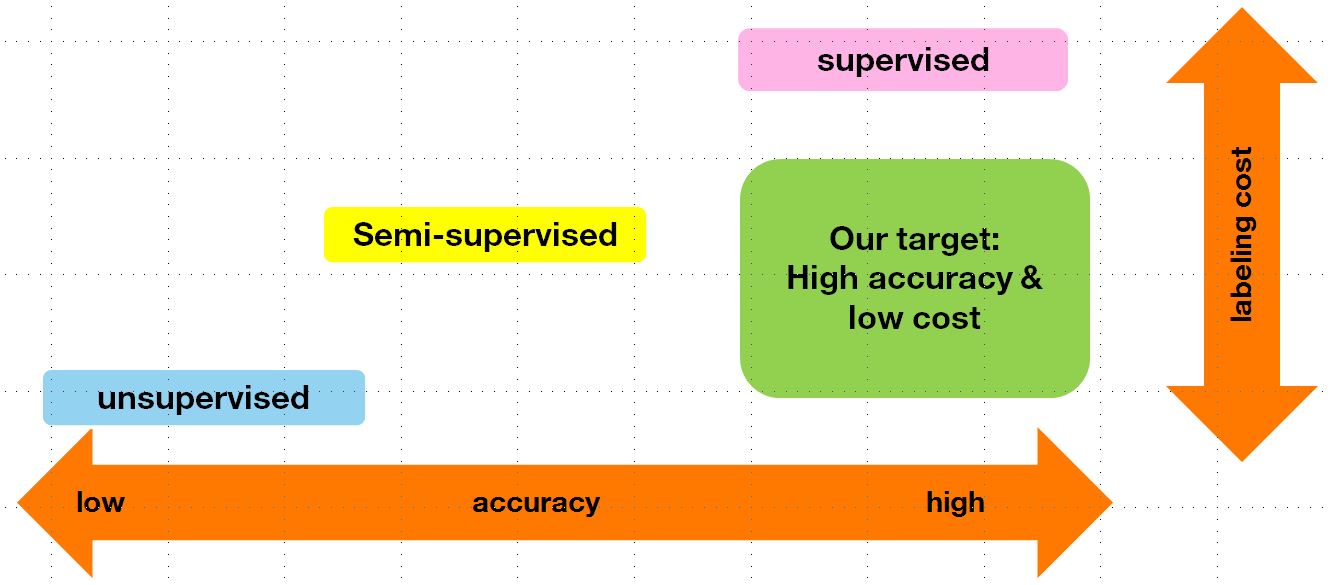
Figure 1: Classification of Classification from [1]

In Weakly Supervised Learning (WSL) use cases (e.g. fraud detection) a variety of situations exist where the collected ground truth is imperfect. In this context, the collected labels may suffer from bad quality, non-adaptability (defined in Section IV) or even insufficient quantity. For instance, automatic labeling system could be used without any real guarantee that the data is complete, exhaustive and trustworthy. Alternatively, manual labelling is also problematic in practice as obtaining labels from an expert is costly and the availability of experts is often limited. Consequently, there are many real-life situations where imperfect ground truth must be used because of some practical considerations such as cost optimization, expert availability, difficulty to certainly choose each label.

This general problem of supervision deficiency has attracted a recent focus in the literature. The paradigm of Weakly Supervised Learning attempts to list and cover these problems with associated solutions. The work of Zhou in [2] is a first successful effort to synthesise this domain. In this paper, the objective is threefold: (i) to suggest another view of WSL, (ii) to propose a larger and updated taxonomy compared to [2], and then (iii) to highlight a new emergent view of a part of the WSL, namely the biquality learning.

The rest of this paper is organized as follows. In Section II, we present the three axis of the Weakly supervised Learning cube and an overview of most of all the elements of their facets. Section III gives additional elements which have to be taken in consideration at the crossroad of these three axes or when dealing with Weakly learning problems. Section IV suggests 3 key concepts which help at summarizing WSL: Quantity, Quality and Adaptability. In Section V, these 3 concepts are used to raise links between some learning frameworks jointly used in WSL as in Biquality Learning. Section VI then give existing works examples of Biquality Learning. Finally the Section VII concludes this paper.

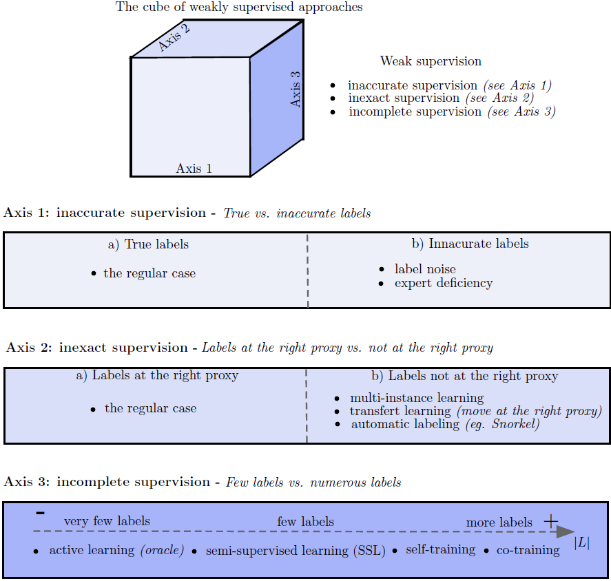
Figure 2: Taxonomy: an attempt - The big picture

II The different ways of looking at weak supervision

The taxonomy proposed in this paper is organised in the form of a “cube” and is presented in Figure 2. This section progressively presents the differences between weakly supervised approaches by going through the axes of this cube.

First of all, a distinction must be made between strong and weak supervision. On the one hand, strong supervision correspond to the regular case in machine learning where the training examples are expected to be exhaustively labelled with true labels, i.e. without any kind of corruption or deficiency. On the other hand, weak supervision means that the available ground truth is imperfect, or even corrupted. The WSL field aims to address a variety of supervision deficiencies which can be categorized in a “cube” along the following three axes as illustrated on Figure 2: inaccurate labels (Axis 1), inexact labels (Axis 2), incomplete labels (Axis 3).

These three axes are detailed in the rest of this section and constitute the proposed taxonomy. The reader may note that the boundaries between these axes are not hard: i.e a part could be moved from an axis to another or belong to two axes, this is a suggestion.

II-A Axis 1: Inaccurate Supervision - True Labels vs. Inaccurate Labels

Lack of confidence in data sources is a frequent issue when it comes to real-life use cases. The values used as learning targets, also called labels or classes, can be incorrect due to many factors.

In practice, a variety of situations can lead to inaccurate labels: (i) a label can be assigned to a “bag of examples ” such as a bunch of keys. In this case, at least one of the examples in the keychain actually belongs to the class indicated by the label. Multi-instance learning [3, 4, 5, 6] is an appropriate technique to deal with this type of of learning task. (ii) a label may not be “guaranteed” and may be noisy. In theory, the learning set should be labeled in a way that is unbiased with respect to the concept to be learned. However, the data used in real-world applications provide an imperfect ground truth that does not match the concept to be learned. As defined in [7], noise is “anything that obscures the relationship between the features of an instance and its class”. According to this definition, every error or imprecision in a attribute or label is considered as noise, including human deficiency. Noise is not a trivial issue because the origin is never clearly obvious. In practical cases, this leads to troubles into evaluating existence and strength level of noise into a dataset. Frenay et al. in [8] provide a good overview of noise sources, impact of labeling noise, types of noise and dependency to noise. Below is a non-exhaustive list of common ways to learn a model in the presence of labeling noise:

• in case of mariginal noise level, a standard learning algorithm that is natively robust to label noise, is used [9, 10, 11, 12];

• use a loss function which solves theoretically (or empirically) the problem in case of (i) noise completely at random [13]; or (ii) class dependent noise [14, 15]. In most cases, this type of approach is known in the literature as “Robust Learning to Label noise (RLL)”;

• model noise to assess the quality of each label (requires assumptions on noise) [16];

• enforce consistency between the model’s predictions and the proxy labels [17];

• clean the training set by filtering noisy examples [18, 19, 20, 21, 22];

• trust a subset of data provided by the user, in order to learn a model at once on trusted examples (without label noise) and untrusted ones [14, 23, 24].

Another kind of ”noise” appears when each training example is not equipped with a single true label but with a set of candidate labels that contains the true label. To deal with this kind of training examples, Partial Label Learning (PLL) has been proposed [25] (also called ambiguously labeled learning). It has attracted attention as for example in the algorithms IPAL [26], PL-KNN [25], CLPL [27] and PL-SVM [28] or when suggesting semi-supervised partial label learning as in [29]. This setting is motivated, for example, by common scenario in many image and video collections, where only partial access to labels is available. The goal is to learn a classifier that can disambiguate the partially-labeled training instances, and generalize to unseen data [30].

II-B Axis 2: Inexact Supervision - Labels at the Right Proxy vs. not at the Right Proxy

The second axis describes inexact labeling which is orthogonal to the first type of supervision deficiency - i.e. inexact labeling and noisy labeling may coexist. Here, the labels are provided not at the right proxy, which corresponds to one (or possibly a mixture) of the following situations:

• Proxy domain: the target domain differs between the training set and the test set. For instance, it could be learning to discriminate “panthers” from other savanna animals based one “cats” and “dogs” labels. Two cases can be distinguished: (i) training labels are available in another target domain than test labels (ii) or training labels are available in a sub-domain that belongs to the original target domain. Domain transfer [31] or domain adaptation [32] are clearly suitable techniques to address these learning tasks.

• Proxy labels: some unlabeled examples are automatically labeled, either by a rule-based system or by a learned model, in order to increase the size of the training set. This kind of labels are called proxy labels and can be considered as coming from a proxy concept close to the one to be learned. Only the true labels stand for the ground truth. The way proxy labels are used varies depending on their origin. In the case where proxy labels are provided by the classifier itself without any additional supervision, the self-training (ST) [33], the co-training (CT) and their variants attempt to improve the learned model by including proxy-labels in the training set as regular labels. Other approaches exploits the confidence level of the classifier to produce soft-proxy-labels, and then exploit it as weighted training examples [34]. In the case where proxy labels are generated by a rule-based system, the quality of labels depends on the experts knowledge which is manually inputted into the rules. Ultimately, a classifier learned from such labels can be considered as a means of smoothing the set of rules, allowing the end-user to score any new example. Some recent automatic labeling system offer an intermediate way that mixes rule-based systems and machine learning approaches (MIX) [35, 36].

• Proxy individuals: the statistical individuals are not equally defined between the training set and the test set. For instance, it could be learning to classify images based one labels that only describe a parts of the images. Multi-instance learning (MIL) is an other example which consists in learning from labeled groups of individuals. In the literature, many algorithms have been adapted to work within this paradigm [3, 4, 5, 6].

II-C Axis 3: Incomplete Supervision - Few labels vs. Numerous

The third axis describes incomplete supervision which consists of processing a partially labeled training set. In this situation, labeled and unlabeled examples coexist within the training set, and it is assumed that there are not enough labeled examples to train a performing classifier. The objective is to use the entire training set, including the unlabeled examples, to achieve better classification performance than learning a classifier only from labeled examples.

In the literature, many techniques exist capable of processing partially labeled training data, i.e. active learning (AL), semi-supervised learning (SSL), positive unlabeled learning (PUL) or self-training (ST) and Co-Training (CT). At the bottom of the Figure 2, we suggest to sort these methods according to the quantity of labeled examples they require. All these approaches are detailed below.

II-C1 Active Learning (AL) [37]

Modern supervised learning approaches are known to require large amounts of training examples in order to achieve their best performance. These examples are mainly obtained by human experts who label them manually, making the labelling process costly in practice. Active learning (AL) is a field that includes all the selection strategies that allow one to iteratively build the training set of a model in interaction with a human expert (also called oracle). The aim is to select the most informative examples to minimize the labelling cost.

Active learning is an iterative process that continues until a labelling budget is exhausted or a predefined performance threshold is reached. Each iteration begins with the selection of the most informative example. This selection is generally based on information collected during previous iterations (predictions of a classifier, density measures, etc.). The selected example is then submitted to the oracle which returns the associated class, and the example is added to the training set ($L$). The new learning set is then used to improve the model and the new predictions are used to perform the next iteration.

In conventional heuristic the utility measures used by active learning strategies [37] differ in their positioning with respect to the trade off between exploiting the current classifier and exploring training data. Selecting an unlabelled example in an unknown region of the observation space helps to explore the data, so as to limit the risk of learning a hypothesis that is too specific to the set $L$ of currently labeled examples. Conversely, selecting an example in an already sampled region allows to locally refine the predictive model. We do not intend to provide an exhaustive overview of existing AL strategies and refer to  [38, 37] for a detailed overview, [39, 40, 41] for some recent benchmark and a new way to treat uncertainty in  [42]

Another meta active learning paradigm exists, which combines conventional strategies using bandit algorithms [43, 44, 45, 46, 47, 48]. These meta-learning algorithms intend to select online the best AL strategy according to the observed improvements of the classifier. These algorithms are capable of adapting their choice over time as the classifier improves. However, learning must be done using few examples to be useful and these kind of algorithms suffer from the cold start problem. In addition these approaches are limited to combine existing AL heuristic strategies.

Other meta-active-learning algorithms have been developed to learn an AL strategy starting from scratch, using multiple source of datasets. These algorithms are used by transferring the learned AL strategy to new target datasets [49, 50, 51]. Most of them are based on modern reinforcement learning methods. The major challenge is to learn an AL strategy general enough to automatically control the exploitation/exploration trade-off when used on new unlabeled datasets (which is impossible using heuristic strategies). A recent evaluation of learning active learning can be found in [52].

II-C2 Semi Supervised Learning (SSL)

Early work on semi-supervised learning dates back to the 2000s, an overview of these pioneering papers can be found in [53, 54, 55, 56, 57]. In the literature, the SSL approaches can be categorized into two groups:

• Algorithms that use unlabeled examples unchanged. In this case, the unlabeled examples are treated as unsupervised information added to the labeled examples. Four main categories exist: generative methods, graph-based methods, low-density separation methods, and disagreement-based methods [2].

• Semi-supervised learning algorithms that produce proxy labels on unlabeled examples, which are used as targets in addition to the labeled examples. These proxy labels are produced by the model itself or by its variantswithout any additional supervision. They are not strictly ground truth, but may nevertheless be useful for learning. At the end, these inaccurate labels (see Section II-A) can be considered as noisy. The rest of this section deals with particular cases of SSL and presents the Postive Unlabeled Learning , the Self Training and the Co-training approaches.

II-C3 Postive Unlabeled Learning (PUL)

Learning from Positive and Unlabeled examples (PUL) is a special case of binary classification and SSL [58]. In this particular setting, the unlabeled examples may contain both positive and negative examples with hidden labels. These approaches differ from a one-class classification [59] since they explicitly use the unlabeled examples in the learning process. In the literature, the PUL approches can be divided into three groups: i) the two-step techniques, (ii) the biased learning and (iii) the class prior incorporation techniques.

The two-step techniques [60] consists in: (1) identifying reliable negative examples and optionally generating additional positive examples [61]; (2) using supervised or semi-supervised learning approaches which process the positively labeled examples, the reliable negatives examples, and the remaining unlabeled examples; (3) (when applicable) selecting the best classifier generated in Step 2. Biased learning approaches consider PU data as fully labeled examples with noisy negative labels. At last, class prior incorporation approaches modify standard learning algorithms by applying the mathematics from the SCAR setup (see Section III-B).

II-C4 Self Training (ST)

Self-training has not a clear definition is the literature, it can be viewed as a “single-view weakly supervised algorithm”. First a classifier is trained from the available labeled examples and then this classifier is used to make predictions and build new proxy labels. Only those examples where confidence in proxy labelling exceeds a certain threshold are added to the training set. Then, the classifier is retrained from the training set enriched with proxy-labels. This process is repeated in an iterative way [33].

II-C5 Co-Training (CT) [62, 63, 64, 65]

Starting from a set of partially labeled examples, co-learning algorithms aim to increase the amount of labeled examples by generating proxy-labels.

Co-training algorithms work by training several classifiers from the initial labeled examples. Then, these classifier are used to make predictions and generate proxy-labels on the unlabeled examples. The most confident predictions on these proxy-labels are then added to the set of labeled data for the next iteration.

One important aspect of co-training is the relationship between the views (the sets of explicative variables) used in learning the different models. The original co-training algorithm [62] states that the independence of the views is required to properly perform automatic labeling. More recent works [66, 67, 68] show that this assumption can be relaxed. Another requirement is to obtain at the iteration step a “reasonable” classifier in terms of performances , this explains why we place co-training on the left of AL and SSL in Figure IV-A. In [69], a study is given on the optimal selection of the co-training parameters.

Co-training can also be considered as a member of ”multi-view training” family in which some other members belong to, such as: Democratic Co-learning [70], Tri-training [71], Asymmetric tri-training [72], Multi-task tri-training [73], which are not described here.

III Other key elements - Beyond the 3 axes

III-A Learning at the crossroad of the three axis

The use of a cube to describe the literature on Weakly Supervised Learning allows us not only to use the axes, but also the volume of the cube to position existing approaches. It is now easy to position more subtly the approaches that are related to several axes at once. For example, Partial Label Learning may be related to two supervision deficiencies: i) inexact supervision, because multiple labels are provided for each training example; ii) inaccurate supervision, because only one of the labels provided is correct. Positioning the PLL on the plane defined by these two axes seems more relevant.

Also, this representation allows to highlight some interesting intersections, between two axes or between an axis and a plane. One of these points of interest is the origin of the three axes, which corresponds to the case where supervision is absolutely inaccurate, imprecise and incomplete, which ultimately amounts to unsupervised learning. Similarly, the point at the opposite end of the cube corresponds to perfectly precise, accurate and complete supervision, which equates to supervised learning.

Finally this representation could provide insights on the reasons of using proven techniques from a particular subfield of Weakly Supervised Learning can be efficient in another one. For instance, DivideMix [74] chooses to reuse the efficient MixUp [75] approach from Semi-Supervised Learning to tackle the problem of Learning with Label Noise. This approach uses Data Augmentation [76] and Model Agreement [77] to estimate labels probabilities and then discard or keep provided labels.

This section is not exhaustive, interested readers will be able to position the approaches of the literature in the cube themselves.

III-B Deficiency Model

The deficiency model describes the nature of the supervision deficiency. It is usually described as a probability measure called $\rho:(x,y)\mapsto\rho(x,y)$, indicating if an example is corrupt or not. $\rho$ can depends on the value the explanatory variables $x\in\mathcal{X}$, the label value $y\in\mathcal{Y}$ or both $(x,y)$. The different types of supervision deficiency described in this section are the following: (i) Completely At Random (CAR), (ii) At Random (AR) and (iii) Not At Random (NAR).

If the probability of being corrupted is the same for all training examples, $\rho:(x,y)\mapsto\rho_{c}$, $\rho_{c}\in[0,1]$, then the supervision deficiency model is Completely At Random (CAR). This implies that the cause of the supervision deficiency data is unrelated to the data. If the probability of being corrupted is the same within classes, $\rho:(x,y)\mapsto\rho_{y}$, $\forall y\in\mathcal{Y}$, $\rho_{y}\in[0,1]$, then the supervision deficiency model is At Random (AR). If neither CAR nor AR holds, then we speak of Not at Random (NAR) model. Here the probability of being corrupted is dependent on both the samples and the label value, $\rho:(x,y)\mapsto\rho(x,y)$. These three deficiency models can be ranked in a descendent manner, having the NAR model being the most complex as it depends on both the instance and label value, which requires a function to model, to CAR model where only one constant is enough to describe it. These models may help practitioner to find links between supervision deficiencies. For example PUL is SSL with only one class labeled, which means that the missingness of the label is linked to the label value, so PUL is an extreme case of SSL AR with $\rho_{0}=1-e$ and $\rho_{1}=e$ (where $e$ is called the propensity score).

AL is another form of SSL where examples are labeled thanks to a strategy, previously labeled instances and the ordered iterative process leading to non-iid labeled data. As such AL is part of the SSL NAR family. We want to reiterate the deficiency model can be applied to any supervision deficiency, even if it has been mostly featured in RLL and in SSL.

III-C Transductive learning vs. Inductive Learning

As we consider WSL framework, one may be tempted to use the test set to guide the choice of the model. But in this case we need to carefully decide if in the future the need of a model to predict on another test (deployment) dataset is required or not: two point of view could be considered transductive learning vs. inductive learning, that is why now we add a note on them.

Training a machine could take many forms as supervised learning, unsupervised learning, active learning, online learning, etc. The number of members is the family is large and new members appear regularly as for example “federative learning”. However one may establish a separation between two constant classes based on the way the user would like to use the “learning machine” at the deployment stage. The user does not want necessarily a predictive model for subsequent use on new data. Because, for example, it has the completeness of the data for the problem to be treated. It is therefore necessary to distinguish between inductive learning and transductive learning.

On one side the goal of inductive learning is, essentially, to learn a function (a model) which will be later used on new data to predict classes (classification) or numerical values (regression). The predictions may be seen as “buy-products” of the model. Induction is reasoning from observed training cases to general rules, which are then applied to the test cases. On the other side the goal of transductive learning the goal is not to obtain a function or a model but only to do predictions on a given test database, and on only on this test of instances. Transduction was introduced by Vladimir Vapnik in the 1990s, motivated by the intuition that transduction is preferable to induction since, induction requires solving a more general problem (inferring a function) before solving a more specific problem (computing outputs for new cases). However the distinction between inductive and transductive learning could be a hazy border for example in case of semi-supervised learning. Knowing this, the view of Zhou in [2] about “pure semi supervised learning” and transductive learning is interesting. The distinction about Transductive learning vs. Inductive Learning concerned most of the learning form included on Figure 2.

IV The 3 common concepts of WSL

Until now we see that many forms of learning and weakness are intertwined. A way to resume their aspect was given on Figure 2. From this point of view one may identified 3 common concepts that are described now.

IV-A Quantity $|L|$

Insufficient quantity of labels or training examples occurs when many training examples are available but only a small portion is labeled, e.g. due to the cost of labelling. For instance, this occurs in the field of cyber security where human forensics is needed to tag attacks. Usually, this issue is addressed by few shot learning (FSL), active learning (AL) [37] semi-supervised learning (SSL) [55] , Self Training, or Co-Training or active learning (AL) which have been described briefly above in this paper. Another way to see the ”quantity” could be the ratio between the number of examples labeled and unlabeled ($p$).

IV-B Quality $q$

In this case, all training examples are labeled but the labels may be corrupted. This usually happens when outsourcing labeling to crowd labeling [78]. The Robust Learning to Label Noise (RLL) approaches tackle this problem [79], with three types of label noise identified: i) the completely at random noise corresponds to a uniform probability of label change ; ii) the class dependent label noise when the probability of label change depends upon each class, with uniform label changes within each class ; iii) the instance dependent label noise is when the probability of label change varies over the input space of the classifier. This last type of label noise is the most difficult to deal with, and typically requires making sometimes strong assumptions on the data.

IV-C Adaptability $a$

This is the case for instance, in Multi Instance Learning (MIL) [3, 4, 5, 6], in which there is one label for each bag of training examples, and each example has an uncertain label. Some scenarios in Transfer Learning (TL) [80] imply that only the labels in the source domain are provided while the target domain labels are not. Often, these non-adapted labels are associated with the existence of slightly different learning tasks (e.g. more precise and numerous classes are dividing the original categories). Alternatively, non-adapted labels may characterize a differing statistical individual [81] (e.g. a subpart of an image instead of the entire image).

V From WSL to Biquality learning (when $a=1$)

All the types of supervision deficiencies presented above are addressed separately in the literature, leading to highly specialized approaches. In practice, it is very difficult to identify the type(s) of deficiencies with which a real dataset is associated. For this reason, it would be very useful to suggest another point of view as a tentative of an unified framework for (a part of the) Weakly Supervised Learning, in order to design generic approaches capable of dealing not a single type of supervision deficiency. This is the purpose of this section mainly given for cases where data are adapted to the task to learn ($a=1$).

Learning using biquality data has recently been put forward in [82, 14, 83] and consists in learning a classifier from two distinct training sets, one trusted and the other not. The initial motivation was to unify semi-supervised and robust learning through a combination of the two. We show in this paper that this scenario is not limited to this unification and that it can cover a larger range of supervision deficiencies as demonstrated with the algorithms we suggest and their results.

The trusted dataset $D_{T}$ consists of pairs of labeled examples ($x_{i},y_{i}$) where all labels $y_{i}\in\mathcal{Y}$ are supposed to be correct according to the true underlying conditional distribution $\mathbb{P}_{T}(Y|X)$. In the untrusted dataset $D_{U}$, examples $x_{i}$ may be associated with incorrect labels. We note $\mathbb{P}_{U}(Y|X)$ the corresponding conditional distribution.

At this stage, no assumption is made about the nature of the supervision deficiencies which could be of any type including label noise, missing labels, concept drift, non-adapted labels … and more generally a mixture of these supervision deficiencies.

The difficulty of a learning task performed on biquality data can be characterised by two quantities. First, the ratio of trusted data over the whole data set, denoted by $p$:

$$\small{p=\frac{|D_{T}|}{|D_{T}|+|D_{U}|}}$$ (1)

Second, a measure of the quality, denoted by $q$, which evaluates the usefulness of the untrusted data $D_{U}$ to learn the trusted concept For example in [83] $q$ is defined using a ratio of Kullback-Leibler divergence between $\mathbb{P}_{T}(Y|X)$ and $\mathbb{P}_{U}(Y|X)$.

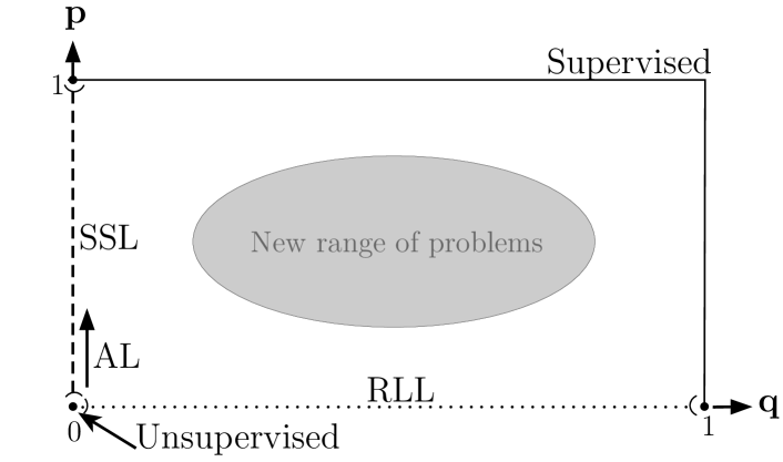
Figure 3: The different learning tasks covered by the biquality setting, represented on a 2D representation.

The biquality setting covers a wide range of learning tasks by varying the quantities $q$ and $p$, as represented in Figure 3.

• When ($p=1$ OR $q=1$) all examples can be trusted. This setting corresponds to a standard supervised learning (SL) task.

• When ($p=0$ AND $q=0$), there is no trusted examples and the untrusted labels are not informative. We are left with only the inputs $\{x_{i}\}_{1\leq i\leq m}$ as in unsupervised learning (UL).

• On the vertical axis defined by $q=0$, except for the two points $(p,q)=(0,0)$ and $(p,q)=(1,0)$, the untrusted labels are not informative, and trusted examples are available. The learning task becomes semi-supervised learning (SSL) with the untrusted examples as unlabeled and the trusted as labeled.

• An upward move on this vertical axis, from a point $(p,q)=(\epsilon,0)$ characterized by a low proportion of labeled examples $p=\epsilon$, to a point $(p^{\prime},0)$, with $p^{\prime}>p$, corresponds to Active Learning, if an oracle can be called on unlabeled examples. The same upward move can also be realized in Self-training and Co-training, where unlabeled training examples are labeled using the predictions of the current classifier(s).

• On the horizontal axis defined by $p=0$, except for the points $(p,q)=(0,0)$ and $(p,q)=(0,1)$, only untrusted examples are provided, which corresponds to the range of learning tasks typically addressed by Robust Learning to Label noise (RLL) approaches.

Only the edges of Figure 3 have been envisioned in previous works – i.e. the points mentioned above – and a whole new range of problems corresponding to the entire plan of the figure remains to be explored. Biquality learning may also be used to tackle particular tasks belonging to WSL, for instance:

• Positive Unlabeled Learning (PUL) [58] where the trusted examples are only positive and untrusted examples those from the unknown class.

• Self Training and Co-training [62, 63, 64] could be adressed at the end of their self labeled process: the initial training set is the trusted dataset, all examples labeled after (during the self labeling process) are the untrusted examples.

• Concept drift [84]: when a concept drift occurs, all the examples used before a drift detection may be considered as the untrusted examples, while the examples available after it are viewed as the trusted ones, assuming a perfect labeling process.

• Self Supervised Learning system as Snorkel [35]: the small initial training set is the trusted dataset, all examples automatically labeled using the labeling functions correspond to the untrusted examples.

As can be seen from the above list, the Biquality framework is quite general and its investigation seems a promising avenue to unify different aspects of the Weakly Supervised Learning.

VI Biquality Learning - Existing Works

In the previous section we have been describing how Wealky Supervised Learning subfields fitted in the Biquality Learning setup. Here we would be reviewing three of these subfields and highlight prexisting Biquality Learning algorithms that either have been made for a different purpose but still could be used for WSL, or have been design directly for this setup.

VI-A Transfer Learning

Transfer Learning focuses on storing, knowledge gained while solving one problem and applying it to a different but related problem. Two datasets are at disposal, a source dataset $D_{S}$ and target dataset $D_{T}$ that are related to a source domain $\mathcal{D}_{S}(\mathcal{X}_{S},\mathbb{P}(X_{S}))$ and a target domain $\mathcal{D}_{T}(\mathcal{X}_{T},\mathbb{P}(X_{T}))$ to solve the target task $\mathcal{T}_{T}(\mathcal{Y}_{T},\mathbb{P}(Y_{T}|X_{T}))$ with the help of the source task $\mathcal{T}_{S}(\mathcal{Y}_{S},\mathbb{P}(Y_{S}|X_{S}))$. We can draw a parallel between Biquality Learning notations and Transfer Learning notations mostly by substituting (source, $S$) by (untrusted, $U$) and (target, $T$) by (trusted, $T$).

A lot of different setups can derive from the general Transfer Learning setup as Domain Adaptation, Transductive Transfer Learning, Covariate Shift, … Inductive Transfer Learning is the setup closest to Biquality Learning, indeed most of the key assumptions are the same : $\mathcal{X}_{T}=\mathcal{X}_{U}$, $\mathcal{Y}_{T}=\mathcal{Y}_{U}$, $\mathbb{P}(X_{T})=\mathbb{P}(X_{U})$, $\mathbb{P}(Y_{T}|X_{T})\neq\mathbb{P}(Y_{U}|X_{U})$.

For example, TrAdaBoost [85] is an extension of boosting to Inductive Transfer Learning. TrAdaBoost learns on both trusted and untrusted data every iterations. It behaves exactly as AdaBoost [86, 87] on trusted data : mispredicted trusted samples get more attention, but opposite on untrusted data : mispredicted untrusted samples are ditched out.

Multi Task Learning [88] is another Inductive Transfer Learning approach that improves generalization by learning both tasks in parallel while using a shared representation; what is learned for the untrusted task can help the trusted task. This loss $L_{\text{MTL}}$ is usually defined by a convex combination of the trusted loss $L_{T}$ and untrusted loss $L_{U}$ of the model $f$ (with $0\leq\lambda\leq 1$):

$$\medmath{L_{\text{MTL}}(f(X),Y)=(1-\lambda)L_{U}(f(X),Y)+\lambda L_{T}(f(X),Y)}$$ (2)

In Inductive Transfer Learning as in Transfer Learning in general, we assume that the source task (i.e. untrusted task) is relevant for the target task (i.e. trusted task). Nonetheless in the Biquality Data setup, we can have the untrusted task that bring no information to the trusted task, even bring adversarial information. Thus using Inductive Transfer Learning algorithm directly on Biquality Data setup can lead to bad predictive performances.

For example, with Multi Task Learning, the global loss term would be heavily perturbed as the untrusted loss could never be optimized. For TrAdaBoost, the first model learned on both trusted and untrusted samples would not be able to learn the class boundaries correctly, and the weight updating schemes would not be efficient.

VI-B RLL and Transition Matrix

A family of Biquality Learning algorithm has been pioneered by Patrini with [89] from the Robust Learning to Label Noise literature. These algorithms try to estimate the per class probabilities of label flip into another class (of the $K$ classes) which defines the Transition Matrix $T$.

$$\medmath{\forall(i,j)\in K^{2},\>T_{(i,j)}=\mathbb{P}(Y_{U}=j|Y_{T}=i)}$$ (3)

Patrini proposed in [89] to used the Transition Matrix $T$ to adapt any supervised loss functions $L$ to learning with label noise. The two corrections proposed are : (i) the forward loss correction: $L^{\rightarrow}(f(X),Y)=L(T^{\top}\cdot f(X),Y)$ and (ii) the backward loss correction: $L^{\leftarrow}(f(X),Y)=T^{-1}\cdot L(f(X),Y)$.

When no trusted samples are available as in [89], Patrini proposed to use anchor points in order to estimate $T$. An anchor point from the $i$-th class is the point with the highest probability to be from the $i$-th class from a given dataset.

$$\medmath{\forall i\in K,\>A_{i}=\operatorname*{argmax}_{x}\mathbb{P}(Y=i|X=x)}$$ (4)

Thanks to this definition Patrini propose an estimator of the Transition Matrix :

$$\medmath{\hat{T}_{(i,j)}=\mathbb{P}(Y=j|X=A_{i})}$$ (5)

Finally the procedure to learn a model $f$ that minimizes $L$ on untrusted data with Patrini’s approach is in two steps. First learn $f$ model on untrusted data with a loss $L$. Estimate the Transition Matrix thanks to $\hat{T}$ with Equation 5. Then learn a model $f$ with either $L^{\rightarrow}$ or $L^{\leftarrow}$.

This algorithm, designed for Robust Learning to Label noise can easily be adapted to Biquality Learning. Hendrycks proposed one adaptation in [14] with some changes to Patrini’s approach. As trusted data are available, there is no more the need to use anchor points to represent our trusted concept. So another estimator for the Transition Matrix is proposed by learning a model $f_{U}$ on untrusted data, and making probabilistic predictions with $f_{U}$ on the trusted dataset $D_{T}$ and comparing it to the trusted labels $y_{T}$ :

$$\medmath{\hat{T}_{(i,*)}=\sum_{x_{i}\in D^{i}_{T}}\frac{f_{U}(x_{i})}{\sum_{z_{i}\in D^{i}_{T}}||f_{U}(z_{i})||}}$$ (6)

where $D^{i}_{T}=\{\forall(x,y)\in D_{T}|y=i\}$. Then for the final step, Hendrycks proposed to learn $f$ with the corrected forward loss $L^{\rightarrow}$ on the untrusted data, and the uncorrected loss $L$ on the trusted data. Thus GLC is an example of a Biquality Learning algorithm that has been demonstrated to be quite efficient on At Random supervision deficiencies.

VI-C Covariate Shift

Covariate Shift literature has also inspired people to adapt these algorithms to Biquality Learning. The algorithm with the most influence in this regard is called Importance Reweighting [90], which aims was to give high weights to source samples that were similar to the target samples, and low weights when they were not similar. This objective fits well with Not At Random (or sample dependent) corruptions as the correction made to the untrusted dataset is per sample with this algorithm family. Multiple approaches has been inspired by this literature.

The key idea of this algorithm family is to define a loss function $\tilde{L}$ such that learning a model $f$ on $D_{U}$ that minimizes $\tilde{L}$ is equivalent to using the original loss function $L$ on $D_{T}$ in the risk estimate. The following equations show how $\tilde{L}$ appears from the risk estimate $R$:

$$\medmath{\begin{aligned} &R_{(X,Y)\sim T,L}(f)=\mathbb{E}_{(X,Y)\sim T}[L(f(X),Y)]\\ &\qquad=\mathbb{E}_{(X,Y)\sim U}[\frac{\mathbb{P}_{T}(X,Y)}{\mathbb{P}_{U}(X,Y)}L(f(X),Y)]\\ &\qquad=\mathbb{E}_{(X,Y)\sim U}[\beta L(f(X),Y)]\\ &\qquad=R_{(X,Y)\sim U,\tilde{L}}(f)\\ \end{aligned}}$$ (7)

However this newly defined loss function $\tilde{L}$ can be hard to estimate and thus approaches have been proposed to further simplify the weight estimation.

For example, Importance Reweighting for Biquality Learning (IRBL) [24] uses the biquality hypothesis that the distribution $\mathbb{P}(X)$ is the same in the trusted and untrusted datasets. By using Bayes Formula we have a new expression for $\beta$ :

$$\medmath{\beta_{\text{IRBL}}=\frac{\mathbb{P}_{T}(X,Y)}{\mathbb{P}_{U}(X,Y)}=\frac{\mathbb{P}_{T}(Y|X)\mathbb{P}(X)}{\mathbb{P}_{U}(Y|X)\mathbb{P}(X)}=\frac{\mathbb{P}_{T}(Y|X)}{\mathbb{P}_{U}(Y|X)}}$$ (8)

First, the vector of ratios between $\mathbb{P}_{T}(Y|X)$ and $\mathbb{P}_{U}(Y|X)$ is estimated by the term ${\small f_{T}(x_{i})\oslash f_{U}(x_{i})}$, using the models $f_{T}$ and $f_{U}$ learn on $D_{T}$ and $D_{U}$. For each untrusted example, the weight $\hat{\beta}_{\text{IRBL}}$ is the $y_{i}$-th element of this vector; while $\hat{\beta}_{\text{IRBL}}$ is fixed to 1 for the trusted examples. Then, the final classifier is learned from $D_{T}\cup D_{U}$ by minimizing $\tilde{L}$.

Another algorithm has been proposed in [91] named Dynamic Importance Reweighting (DIW) by writing Equation 8 in a more traditional way with Bayes Formula.

$$\medmath{\beta_{\text{DIW}}=\frac{\mathbb{P}_{T}(X,Y)}{\mathbb{P}_{U}(X,Y)}\;=\;\frac{\mathbb{P}_{T}(X|Y)\mathbb{P}_{T}(Y)}{\mathbb{P}_{U}(X|Y)\mathbb{P}_{U}(Y)}}$$ (9)

To estimate $\beta_{\text{DIW}}$, the trick is to select both sub-samples of $D_{T}$ and $D_{U}$ with samples of the same classes and then use an Density Ratio Estimator [92] such as Kernel Mean Matching (KMM) [93, 94]. Then a final classifier is learned on $D_{U}$ by minimizing $\tilde{L}$. One particular issue of this algorithm is that KMM is learned by optimizing a quadratic program, $K$-times per batch, that leads to high algorithm complexity especially in the case of massive multiclass classification.

IRBL and DIW are two new Biquality Learning algorithms that work on NAR cases.

VII Concluding remarks

In this paper, we propose a unified view of Weak Supervised Learning to cope with the shortcomings of the supervision in the field of Machine Learning. We discussed these shortcomings through a cube along with three axes corresponding to the characteristics of training labels (inaccurate, inexact and incomplete). The detailed presentation of these axes gives an insight the different existing learning approaches which can be more subtly position on the cube. In this way, the links between some subfields of WSL with Biquality Learning are highlighted, showing how the algorithms of the latter field can be used within the framework of WSL.

References

- [1] M. Sugiyama, “Talk: Recent advances in weakly-supervised learning and reliable learning,” 2019. [Online]. Available: https://portal.klewel.com/watch/webcast/recent-advances-in-weakly-supervised-learning-and-reliable-learning/talk/1/
- [2] Z.-H. Zhou, “A brief introduction to weakly supervised learning,” National Science Review, vol. 5, no. 1, pp. 44–53, 08 2017.
- [3] J. Yang, “Review of multi-instance learning and its applications,” Technical report, School of Computer Science Carnegie Mellon University, 2005.
- [4] Z.-H. Zhou, “Multi-instance learning from supervised view,” Journal of Computer Science and Technology, vol. 21, no. 5, pp. 800–809, 2006.
- [5] J. R. Foulds and E. Frank, “A review of multi-instance learning assumptions,” The Knowledge Engineering Review, 2010.
- [6] M.-A. Carbonneau, V. Cheplygina, E. Granger, and G. Gagnon, “Multiple instance learning: A survey of problem characteristics and applications,” Pattern Recognition, vol. 77, p. 329–353, May 2018.
- [7] R. J. Hickey, “Noise modelling and evaluating learning from examples,” Artificial Intelligence, vol. 82, no. 1-2, pp. 157–179, 1996.
- [8] B. Frenay and M. Verleysen, “Classification in the Presence of Label Noise: A Survey,” IEEE Transactions on Neural Networks and Learning Systems, vol. 25, no. 5, pp. 845–869, 1994.
- [9] H. Le Baher, V. Lemaire, and R. Trinquart, “On the intrinsic robustness of some leading classifiers and symetric loss function - an empiricalevaluation (under review),” arXiv:2010.13570 [cs.LG], 2020.
- [10] D. F. Nettleton, A. Orriols-Puig, and A. Fornells, “A study of the effect of different types of noise on the precision of supervised learning techniques,” Artificial Intelligence Review, vol. 33, no. 4, pp. 275–306, 2010.
- [11] A. Folleco, T. M. Khoshgoftaar, J. Van Hulse, and L. Bullard, “Identifying learners robust to low quality data,” in 2008 IEEE International Conference on Information Reuse and Integration, 2008, pp. 190–195.
- [12] X. Zhu and X. Wu, “Class noise vs. attribute noise: A quantitative study of their impacts,” Artif. Intell. Rev., vol. 22, no. 3, p. 177–210, Nov. 2004.
- [13] N. Charoenphakdee, J. Lee, and M. Sugiyama, “On symmetric losses for learning from corrupted labels,” in International Conference on Machine Learning, vol. 97, 2019, pp. 961–970.
- [14] D. Hendrycks, M. Mazeika, D. Wilson, and K. Gimpel, “Using trusted data to train deep networks on labels corrupted by severe noise,” in Advances in Neural Information Processing Systems 31, 2018, pp. 10 456–10 465.
- [15] X. Xia, T. Liu, N. Wang, B. Han, C. Gong, G. Niu, and M. Sugiyama, “Are anchor points really indispensable in label-noise learning?” in NeurIPS, 2019.
- [16] S. Sukhbaatar, J. Bruna, M. Paluri, L. D. Bourdev, and R. Fergus, “Training convolutional networks with noisy labels,” arXiv: Computer Vision and Pattern Recognition, 2014.
- [17] S. Reed, H. Lee, D. Anguelov, C. Szegedy, D. Erhan, and A. Rabinovich, “Training deep neural networks on noisy labels with bootstrapping,” CoRR, vol. abs/1412.6596, 2015.
- [18] J.-w. Sun, F.-y. Zhao, C.-j. Wang, and S.-f. Chen, “Identifying and Correcting Mislabeled Training Instances,” in Future Generation Communication and Networking (FGCN 2007), vol. 1, Dec. 2007, pp. 244–250, iSSN: 2153-1463.
- [19] A. Malossini, E. Blanzieri, and R. T. Ng, “Detecting potential labeling errors in microarrays by data perturbation,” Bioinformatics, vol. 22, no. 17, pp. 2114–2121, 2006.
- [20] A. L. B. Miranda, L. P. F. Garcia, A. C. P. L. F. Carvalho, and A. C. Lorena, “Use of Classification Algorithms in Noise Detection and Elimination,” in Hybrid Artificial Intelligence Systems, ser. Lecture Notes in Computer Science, 2009, pp. 417–424.
- [21] N. Matic, I. Guyon, L. Bottou, J. Denker, and V. Vapnik, “Computer aided cleaning of large databases for character recognition,” in Proceedings., 11th IAPR International Conference on Pattern Recognition. Vol.II. Conference B: Pattern Recognition Methodology and Systems, Aug. 1992, pp. 330–333.
- [22] J. Van Hulse and T. Khoshgoftaar, “Knowledge Discovery from Imbalanced and Noisy Data,” Data & Knowledge Engineering, vol. 68, no. 12, pp. 1513–1542, Dec. 2009.
- [23] D. Hendrycks, M. Mazeika, S. Kadavath, and D. Song, “Using self-supervised learning can improve model robustness and uncertainty,” in Advances in Neural Information Processing Systems 32, H. Wallach, H. Larochelle, A. Beygelzimer, F. d'Alché-Buc, E. Fox, and R. Garnett, Eds. Curran Associates, Inc., 2019, pp. 15 663–15 674.
- [24] P. Nodet, V. Lemaire, A. Bondu, and A. Cornuéjols, “Importance reweighting for biquality learning,” in Proceedings of the International Joint Conference on Neural Networks (IJCNN), 2021.
- [25] E. Hüllermeier and J. Beringer, “Learning from ambiguously labeled examples,” in Advances in Intelligent Data Analysis VI, A. F. Famili, J. N. Kok, J. M. Peña, A. Siebes, and A. Feelders, Eds. Springer Berlin Heidelberg, 2005, pp. 168–179.
- [26] M.-L. Zhang and F. Yu, “Solving the partial label learning problem: An instance-based approach.” in IJCAI, 2015, pp. 4048–4054.
- [27] T. Cour, B. Sapp, and B. Taskar, “Learning from partial labels,” The Journal of Machine Learning Research, vol. 12, pp. 1501–1536, 2011.
- [28] N. Nguyen and R. Caruana, “Classification with partial labels,” in Proceedings of the 14th ACM SIGKDD international conference on Knowledge discovery and data mining, 2008, pp. 551–559.
- [29] Q.-W. Wang, Y.-F. Li, and Z.-H. Zhou, “Partial label learning with unlabeled data,” in Proceedings of the Twenty-Eighth International Joint Conference on Artificial Intelligence, IJCAI-19, 2019, pp. 3755–3761.
- [30] T. Cour, B. Sapp, and B. Taskar, “Learning from partial labels,” Journal of Machine Learning Research, vol. 12, no. 42, pp. 1501–1536, 2011. [Online]. Available: http://jmlr.org/papers/v12/cour11a.html
- [31] L. Duan, I. W. Tsang, and D. Xu, “Domain transfer multiple kernel learning,” IEEE Transactions on Pattern Analysis and Machine Intelligence, vol. 34, no. 3, pp. 465–479, 2012.
- [32] S. Ben-David, J. Blitzer, K. Crammer, A. Kulesza, F. Pereira, and J. W. Vaughan, “A theory of learning from different domains,” Machine learning, vol. 79, no. 1-2, pp. 151–175, 2010.
- [33] A. Ennaji, D. Mammass, M. El Yassa et al., “Self-training using a k-nearest neighbor as a base classifier reinforced by support vector machines,” International Journal of Computer Applications, vol. 975, p. 8887, 2012.
- [34] L. Torgo, S. Matwin, N. Japkowicz, B. Krawczyk, N. Moniz, and P. Branco, “2nd workshop on learning with imbalanced domains: Preface,” in Second International Workshop on Learning with Imbalanced Domains: Theory and Applications, 2018, pp. 1–7.
- [35] A. Ratner, S. H. Bach, H. Ehrenberg, J. Fries, S. Wu, and C. Ré, “Snorkel: Rapid training data creation with weak supervision,” The VLDB Journal, vol. 29, no. 2, pp. 709–730, 2020.
- [36] P. Varma and C. Ré, “Snuba: Automating weak supervision to label training data,” in International Conference on Very Large Data Bases, vol. 12, no. 3, 2018.
- [37] B. Settles, “Active learning literature survey,” University of Wisconsin-Madison Department of Computer Sciences, Tech. Rep., 2009.
- [38] C. C. Aggarwal, X. Kong, Q. Gu, J. Han, and P. S. Yu, “Active Learning: A Survey,” in Data Classification: Algorithms and Applications, C. C. Aggarwal, Ed. CRC Press, 2014, ch. 22, pp. 571–605.
- [39] D. Pereira-Santos and A. C. de Carvalho, “Comparison of Active Learning Strategies and Proposal of a Multiclass Hypothesis Space Search,” in Proceedings of the 9th International Conference on Hybrid Artificial Intelligence Systems – Volume 8480. Springer-Verlag, 2014, pp. 618–629.
- [40] Y. Yang and M. Loog, “A benchmark and comparison of active learning for logistic regression,” Pattern Recognition, vol. 83, pp. 401–415, 2018.
- [41] D. Pereira-Santos, R. B. C. Prudêncio, and A. C. de Carvalho, “Empirical investigation of active learning strategies,” Neurocomputing, vol. 326–327, pp. 15–27, 2019.
- [42] E. Hüllermeier and W. Waegeman, “Aleatoric and Epistemic Uncertainty in Machine Learning: An Introduction to Concepts and Methods,” arXiv:1910.09457 [cs.LG], 2019.
- [43] Y. Baram, R. El-Yaniv, and K. Luz, “Online Choice of Active Learning Algorithms,” Journal of Machine Learning Research, vol. 5, pp. 255–291, 2004.
- [44] S. Ebert, M. Fritz, and B. Schiele, “Ralf: A reinforced active learning formulation for object class recognition,” in 2012 IEEE Conference on Computer Vision and Pattern Recognition, 2012, pp. 3626–3633.
- [45] W.-N. Hsu and H.-T. Lin, “Active Learning by Learning,” in Proceedings of the Twenty-Ninth AAAI Conference on Artificial Intelligence. AAAI Press, 2015, pp. 2659–2665.
- [46] H.-M. Chu and H.-T. Lin, “Can Active Learning Experience Be Transferred?” 2016 IEEE 16th International Conference on Data Mining, pp. 841–846, 2016.
- [47] T. Collet, “Optimistic Methods in Active Learning for Classification,” Ph.D. dissertation, Université de Lorraine, 2018.
- [48] K. Pang, M. Dong, Y. Wu, and T. M. Hospedales, “Dynamic Ensemble Active Learning: A Non-Stationary Bandit with Expert Advice,” in Proceedings of the 24th International Conference on Pattern Recognition, 2018, pp. 2269–2276.
- [49] K. Konyushkova, R. Sznitman, and P. Fua, “Learning Active Learning from Data,” in Advances in Neural Information Processing Systems 30, 2017, pp. 4225–4235.
- [50] ——, “Discovering General-Purpose Active Learning Strategies,” arXiv:1810.04114 [cs.LG], 2019.
- [51] K. Pang, M. Dong, Y. Wu, and T. M. Hospedales, “Meta-Learning Transferable Active Learning Policies by Deep Reinforcement Learning,” arXiv:1806.04798 [cs.LG], 2018.
- [52] L. Desreumaux and V. Lemaire, “Learning active learning at the crossroads? evaluation and discussion,” in Workshop Interactive Adaptative Learning held at European Conference on Machine Learning, 2020.
- [53] M. Seeger, “Learning with labeled and unlabeled data,” Tech. Rep., 2000.
- [54] O. Chapelle, B. Schölkopf, and A. Zien, Eds., Semi-supervised learning, ser. Adaptive computation and machine learning. Cambridge, Mass: MIT Press, 2006, oCLC: ocm64898359.
- [55] O. Chapelle, B. Scholkopf, and A. Zien, “Semi-supervised learning,” IEEE Transactions on Neural Networks, vol. 20, no. 3, pp. 542–542, 2009.
- [56] X. J. Zhu, “Semi-supervised learning literature survey,” University of Wisconsin-Madison Department of Computer Sciences, Tech. Rep., 2005.
- [57] Z.-H. Zhou and M. Li, “Semi-supervised learning by disagreement,” Knowledge and Information Systems, vol. 24, no. 3, pp. 415–439, 2010.
- [58] J. Bekker and J. Davis, “Learning from positive and unlabeled data: a survey,” Machine Learning, vol. 109, pp. 719–760, 2020.
- [59] S. S. Khan and M. G. Madden, “One-class classification: taxonomy of study and review of techniques,” The Knowledge Engineering Review, vol. 29, no. 3, pp. 345–374, 2014.
- [60] B. Liu, Y. Dai, X. Li, W. S. Lee, and P. S. Yu, “Building text classifiers using positive and unlabeled examples,” in Third IEEE International Conference on Data Mining. IEEE, 2003, pp. 179–186.
- [61] G. P. C. Fung, J. X. Yu, H. Lu, and P. S. Yu, “Text classification without negative examples revisit,” IEEE Trans. on Knowl. and Data Eng., vol. 18, no. 1, p. 6–20, 2006.
- [62] A. Blum and T. Mitchell, “Combining labeled and unlabeled data with co-training,” in Proceedings of the eleventh annual conference on Computational learning theory, 1998, pp. 92–100.
- [63] M. Davy, “A review of active learning and co-training in text classification,” Trinity College Dublin, Department of Computer Science, Tech. Rep., 2005.
- [64] J. Zhao, X. Xie, X. Xu, and S. Sun, “Multi-view learning overview: Recent progress and new challenges,” Information Fusion, vol. 38, pp. 43–54, 2017.
- [65] R. Mihalcea, “Co-training and self-training for word sense disambiguation,” in CoNLL, 2004.
- [66] K. Nigam and R. Ghani, “Analyzing the effectiveness and applicability of co-training,” in Proceedings of the ninth international conference on Information and knowledge management, 2000, pp. 86–93.
- [67] S. P. Abney, “Bootstrapping,” in Proceedings of the 40th Annual Meeting of the Association for Computational Linguistics, July 6-12, 2002, Philadelphia, PA, USA. ACL, 2002, pp. 360–367.
- [68] S. Clark, J. R. Curran, and M. Osborne, “Bootstrapping pos-taggers using unlabelled data,” in Proceedings of the Seventh Conference on Natural Language Learning, CoNLL 2003, Held in cooperation with HLT-NAACL 2003, Edmonton, Canada, May 31 - June 1, 2003. ACL, 2003, pp. 49–55.
- [69] V. Ng and C. Cardie, “Weakly supervised natural language learning without redundant views,” in Proceedings of the 2003 Human Language Technology Conference of the North American Chapter of the Association for Computational Linguistics, 2003, pp. 173–180. [Online]. Available: https://www.aclweb.org/anthology/N03-1023
- [70] Y. Zhou and S. A. Goldman, “Democratic co-learning,” 16th IEEE International Conference on Tools with Artificial Intelligence, pp. 594–602, 2004.
- [71] Zhi-Hua Zhou and Ming Li, “Tri-training: exploiting unlabeled data using three classifiers,” IEEE Transactions on Knowledge and Data Engineering, vol. 17, no. 11, pp. 1529–1541, 2005.
- [72] K. Saito, Y. Ushiku, and T. Harada, “Asymmetric tri-training for unsupervised domain adaptation,” in International Conference on Machine Learning, 2017, pp. 2988–2997.
- [73] S. Ruder and B. Plank, “Strong baselines for neural semi-supervised learning under domain shift,” in Proceedings of the 56th Annual Meeting of the Association for Computational Linguistics (Volume 1: Long Papers), Jul. 2018, pp. 1044–1054.
- [74] J. Li, R. Socher, and S. C. H. Hoi, “Dividemix: Learning with noisy labels as semi-supervised learning,” 2020.
- [75] H. Zhang, M. Cisse, Y. N. Dauphin, and D. Lopez-Paz, “mixup: Beyond empirical risk minimization,” 2018.
- [76] C. Shorten and T. M. Khoshgoftaar, “A survey on image data augmentation for deep learning,” Journal of Big Data, vol. 6, no. 1, p. 60, 2019.
- [77] S. Qiao, W. Shen, Z. Zhang, B. Wang, and A. Yuille, “Deep co-training for semi-supervised image recognition,” in Proceedings of the european conference on computer vision (eccv), 2018, pp. 135–152.
- [78] R. Urner, S. B. David, and O. Shamir, “Learning from weak teachers,” in Proceedings of the Fifteenth International Conference on Artificial Intelligence and Statistics, ser. Proceedings of Machine Learning Research, vol. 22, pp. 1252–1260.
- [79] B. Frénay and M. Verleysen, “Classification in the presence of label noise: a survey,” IEEE transactions on neural networks and learning systems, vol. 25, no. 5, pp. 845–869, 2013.
- [80] K. Weiss, T. M. Khoshgoftaar, and D. Wang, “A survey of transfer learning,” Journal of Big data, vol. 3, no. 1, p. 9, 2016.
- [81] D. Conte, P. Foggia, G. Percannella, F. Tufano, and M. Vento, “A method for counting people in crowded scenes,” in 2010 7th IEEE International Conference on Advanced Video and Signal Based Surveillance, 2010, pp. 225–232.
- [82] M. Charikar, J. Steinhardt, and G. Valiant, “Learning from untrusted data,” in Proceedings of the 49th Annual ACM SIGACT Symposium on Theory of Computing, 2017, p. 47–60.
- [83] R. Hataya and H. Nakayama, “Unifying semi-supervised and robust learning by mixup,” in The 2nd Learning from Limited Labeled Data Workshop, ICLR, 2019.
- [84] J. a. Gama, I. Žliobaitundefined, A. Bifet, M. Pechenizkiy, and A. Bouchachia, “A survey on concept drift adaptation,” ACM Comput. Surv., vol. 46, no. 4, Mar. 2014. [Online]. Available: https://doi.org/10.1145/2523813
- [85] W. Dai, Q. Yang, G.-R. Xue, and Y. Yu, “Boosting for transfer learning,” in Proceedings of the 24th international conference on Machine learning, 2007, pp. 193–200.
- [86] Y. Freund and R. E. Schapire, “A decision-theoretic generalization of on-line learning and an application to boosting,” Journal of computer and system sciences, vol. 55, no. 1, pp. 119–139, 1997.
- [87] T. Hastie, S. Rosset, J. Zhu, and H. Zou, “Multi-class adaboost,” Statistics and its Interface, vol. 2, no. 3, pp. 349–360, 2009.
- [88] R. Caruana, “Multitask learning,” Machine learning, vol. 28, no. 1, pp. 41–75, 1997.
- [89] G. Patrini, A. Rozza, A. Menon, R. Nock, and L. Qu, “Making deep neural networks robust to label noise: a loss correction approach,” in IEEE Conference on Computer Vision and Pattern Recognition (CVPR), 2017.
- [90] L. Bruzzone and M. Marconcini, “Domain adaptation problems: A dasvm classification technique and a circular validation strategy,” IEEE Transactions on Pattern Analysis and Machine Intelligence, vol. 32, no. 5, pp. 770–787, 2010.
- [91] T. Fang, N. Lu, G. Niu, and M. Sugiyama, “Rethinking importance weighting for deep learning under distribution shift,” 2020.
- [92] M. Sugiyama, T. Suzuki, and T. Kanamori, “Density ratio estimation: A comprehensive review (statistical experiment and its related topics),” 2010.
- [93] J. Huang, A. Gretton, K. Borgwardt, B. Schölkopf, and A. J. Smola, “Correcting sample selection bias by unlabeled data,” in Advances in neural information processing systems, 2007, pp. 601–608.
- [94] A. Gretton, A. Smola, J. Huang, M. Schmittfull, K. Borgwardt, and B. Schölkopf, “Covariate shift by kernel mean matching,” Dataset shift in machine learning, vol. 3, no. 4, p. 5, 2009.