Towards room-temperature superconductivity

Abstract

By taking advantage of a stability criterion established recently, the critical temperature $T_{c}$ is reckoned with help of the microscopic parameters, characterising the normal and superconducting electrons, namely the independent-electron band structure and a repulsive two-electron force. The emphasis is laid on the sharp $T_{c}$ dependence upon electron concentration and inter-electron coupling, which might offer a practical route toward higher $T_{c}$ values and help to understand why high-$T_{c}$ compounds exhibit such remarkable properties.

The BCS theorysch , despite its impressive success, does not enable one to predictmat superconductivity occurring in any metallic compound. Such a drawback ensues from an attractive interaction, assumed to couple electrons together, which is not only at loggerheads with the sign of the Coulomb repulsion but in addition leads to questionable conclusions to be discussed below. Therefore this work is intended at investigating the $T_{c}$ dependence upon the parameters, characterising the motion of electrons correlated together through a repulsive force, within the framework of a two-fluid picturesz8 to be recalled below.

The conduction electrons comprise bound and independent electrons, in respective temperature dependent concentration $c_{s}(T),c_{n}(T)$, such that $c_{0}=c_{s}(T)+c_{n}(T)$ with $c_{0}$ being the total concentration of conduction electrons. They are organized, respectively, as a many bound electronsz5 (MBE) state, characterised by its chemical potential $\mu(c_{s})$, and a Fermi gasash of Fermi energy $E_{F}(T,c_{n})$. The Helmholz free energy of independent electrons per unit volume $F_{n}$ and $E_{F}$ on the one hand, and the eigenenergy per unit volume $\mathcal{E}_{s}(c_{s})$ of bound electrons and $\mu$ on the other hand, are relatedash ; lan , respectively, by $E_{F}=\frac{\partial F_{n}}{\partial c_{n}}$ and $\mu=\frac{\partial\mathcal{E}_{s}}{\partial c_{s}}$. Then a stable equilibrium is conditionedsz4 by Gibbs and Duhem’s law

$$E_{F}(T,c_{n}(T))=\mu(c_{s}(T))\quad,$$ (1)

which expresseslan that the total free energy $F_{n}+\mathcal{E}_{s}$ is minimum provided $\frac{\partial E_{F}}{\partial c_{n}}+\frac{\partial\mu}{\partial c_{s}}>0$. Noteworthy is that $\frac{\partial\mu}{\partial c_{s}}<0$ has been shown to be a prerequisite for persistent currentssz4 , thermal equilibriumsz5 , the Josephson effectsz6 and a stablesz8 superconducting phase. Likewise, Eq.(1) readssz5 ; sz4 for $T=T_{c}$

$$E_{F}(T_{c},c_{0})=\mu(c_{s}=0)=\varepsilon_{b}/2\quad,$$ (2)

with $\varepsilon_{b}$ being the energy of a bound electron pairsz5 . Note that Eqs.(1,2) are consistent with the superconducting transition being of second orderlan , whereas it has been shownsz5 to be of first order at $T<T_{c}$ ($\Rightarrow E_{F}(T,c_{0}-c_{s})\neq\mu(c_{s})$), if the sample is flown through by a finite current.

The binding energysz5 of the superconducting state $E_{b}(T<T_{c})$ has been worked out as

$$E_{b}(T)=\int_{T}^{T_{c}}\left(C_{s}(u)-C_{n}(u)\right)du\quad,$$

with $C_{s}(T),C_{n}(T)$ being the electronic specific heat of a superconductor, flown through by a vanishing currentsz5 and that of a degenerate Fermi gasash . A stable phase ($\Rightarrow E_{b}>0$) requires $C_{s}(T_{c})>C_{n}(T_{c})$, which can be securedsz8 only by fulfilling the following condition

$$\frac{\partial E_{F}}{\partial c_{n}}(T_{c},c_{0})=-\frac{\partial\mu}{\partial c_{s}}(0),\quad\rho^{\prime}(E_{F}(T_{c},c_{0}))>0\quad,$$ (3)

with $\rho\left(\epsilon\right),\epsilon$ being the independent electron density of states and one-electron energy, respectively, and $\rho^{\prime}=\frac{d\rho}{d\epsilon}$.

Since the remaining analysis relies heavily on Eqs.(2,3), explicit expressions are needed for $E_{F}(T_{c},c_{0}),\frac{\partial E_{F}}{\partial c_{n}}(T_{c},c_{0}),\varepsilon_{b},\frac{\partial\mu}{\partial c_{s}}(0)$. Because the independent electrons make up a degenerate Fermi gas ($\Rightarrow T<<E_{F}/k_{B}$ with $k_{B}$ being Boltzmann’s constant), applying the Sommerfeld expansionash up to $T^{2}$ yields

$$\begin{array}[]{c}E_{F}(T_{c},c_{0})=E_{F}(0,c_{0})-\frac{\rho^{\prime}}{\rho}\frac{\left(\pi k_{B}T_{c}\right)^{2}}{6}\\ \frac{\partial E_{F}}{\partial c_{n}}(T_{c},c_{0})=\left(\rho+\rho^{\prime\prime}\frac{\left(\pi k_{B}T_{c}\right)^{2}}{6}\right)^{-1}\end{array}\quad,$$ (4)

with $\rho=\rho(E_{F}(0,c_{0})),\rho^{\prime}=\frac{d\rho}{dE_{F}}(E_{F}(0,c_{0})),\rho^{\prime\prime}=\frac{d^{2}\rho}{dE_{F}^{2}}(E_{F}(0,c_{0}))$. As for $\varepsilon_{b},\frac{\partial\mu}{\partial c_{s}}(0)$, a truncated Hubbard Hamiltonian $H_{K}$, introduced previouslyja1 ; ja2 ; ja3 , will be used. The main features of the calculationsz5 are summarised below for self-containedness.

The independent electron motion is described by the Hamiltonian $H_{d}$

$$H_{d}=\sum_{k,\sigma}\epsilon(k)c^{+}_{k,\sigma}c_{k,\sigma}\quad.$$

$\epsilon(k),k$ are the one-electron energy ($\epsilon(k)=\epsilon(-k)$) and a vector of the Brillouin zone, respectively, $\sigma=\pm$ is the electron spin and the sum over $k$ is to be carried out over the whole Brillouin zone. Then $c^{+}_{k,\sigma},c_{k,\sigma}$ are creation and annihilation operators on the Bloch state $\left|k,\sigma\right\rangle$

$$\left|k,\sigma\right\rangle=c^{+}_{k,\sigma}\left|0\right\rangle\quad,\quad\left|0\right\rangle=c_{k,\sigma}\left|k,\sigma\right\rangle\quad,$$

with $\left|0\right\rangle$ being the no electron state. The Hamiltonian $H_{K}$ reads then

$$H_{K}=H_{d}+\frac{U}{N}\sum_{k,k^{\prime}}c^{+}_{k,+}c^{+}_{K-k,-}c_{K-k^{\prime},-}c_{k^{\prime},+}\quad,$$

with $N>>1,U>0$ being the number of atomic sites, making up the three-dimensional crystal, and the Hubbard constant, respectively. Note that the Hamiltonian used by Coopercooper is identical to $H_{K=0}$, but with $U<0$.

$H_{K}$ sustainssz5 a single bound pair eigenstate, the energy $\varepsilon_{b}(K)$ of which is obtained by solving

$$\frac{1}{U}=\frac{1}{N}\sum_{k}\frac{1}{\varepsilon_{b}(K)-\varepsilon(K,k)}=\int_{-t_{K}}^{t_{K}}\frac{\rho_{K}(\varepsilon)}{\varepsilon_{b}(K)-\varepsilon}d\varepsilon.$$ (5)

$\pm t_{K}$ are the upper and lower bounds of the two-electron band, i.e. the maximum and minimum of $\varepsilon(K,k)=\epsilon(k)+\epsilon(K-k)$ over $k$, whereas $\rho_{K}(\varepsilon)$ is the corresponding two-electron density of states, taken equal to

$$\rho_{K}(\varepsilon)=\frac{2}{\pi t_{K}}\sqrt{1-\left(\frac{\varepsilon}{t_{K}}\right)^{2}}\quad.$$

The dispersion curves $\varepsilon_{b}(K)$ are plotted in Fig.11. Though Eq.(5) is identical to the equation yielding the Cooper pair energycooper , their respective properties are quite different :

• the data in Fig.11 have been calculated with $U>0$, rather than $U<0$ favoured by Coopercooper and BCSsch , because, due to the inequalitysz5 $U\frac{\partial\mu}{\partial c_{s}}<0$, choosing $U<0$ entails $\frac{\partial\mu}{\partial c_{s}}>0$, which has been shown not to be consistent with persistent currentssz4 , thermal equilibriumsz5 , the Josephson effectsz6 and occurencesz8 of superconductivity. As a further consequence of $U>0$, $\varepsilon_{b}(K)$ shows up in the upper gap of the two-electron band structure ($\Rightarrow\varepsilon_{b}(K)>t_{K}$) rather than in the lower gap ($\Rightarrow\varepsilon_{b}(K=0)<-t_{K}$) in case of the Cooper paircooper . Nevertheless the bound pair is thermodynamically stable, because every one-electron state of energy $<E_{F}(T_{c},c_{0})$, is actually occupied, so that, due to Pauli’s principle, a bound electron pair of energy $\varepsilon_{b}(K)=2E_{F}(T_{c},c_{0})$, according to Eq.(2), cannot decay into two one-electron states $\epsilon(k)<E_{F},\epsilon(K-k)<E_{F}$;

• a remarkable feature in Fig.11 is that $\varepsilon_{b}(K)\rightarrow t_{K}$ for $U\rightarrow t_{K}/2$, so that there is no bound pair for $U<t_{K}/2$ (accordingly, the dashed curve is no longer defined in Fig.11 for $\frac{Ka}{\pi}<.13$), in marked contrast with the opposite conclusion drawn by Coopercooper , that there is a Cooper pair, even for $U\rightarrow 0$. This discrepancy results from the three-dimensional Van Hove singularities, showing up at both two-electron band edges $\rho_{K}\left(\varepsilon\rightarrow\pm t_{K}\right)\propto\sqrt{t_{K}-\left|\varepsilon\right|}$, unlike the two-electron density of states, used by Coopercooper which is constant and thence displays no such singularity. Likewise the width of Cooper’s two-electron band is equal to a Debye phonon energy $2t_{K=0}=\omega_{D}\approx 30meV<<E_{F}\approx 3eV$. Hence the resulting small concentration of superconducting electrons, $\frac{c_{s}(T=0)}{c_{0}}\approx\frac{\omega_{D}}{E_{F}}\approx.01$, entails that London’s length should be at least $10$ times larger than observed valuessz1 ; sz2 ; sz3 ; sz7 ;

• at last Cooper’s assumption $U<0$ implies $\varepsilon_{b}/2\neq E_{F}(T_{c})$, which is typical of a first order transition but runs afoul at all measurements, proving conversely the superconducting transition to be of second order ($\Rightarrow\varepsilon_{b}/2=E_{F}(T_{c})$ in accordance with Eq.(2)).

The bound pair of energy $\varepsilon_{b}(K)$ turns, at finite concentration $c_{s}$, into a MBE state, characterised by $\mu(c_{s})$. Its properties have been calculated thanks to a variational proceduresz5 , displaying several merits with respect to that used by BCSsch :

• it shows that $\mu(0)=\varepsilon_{b}/2$;

• the energy of the MBE state has been shown to be exact for $\left|U\right|\rightarrow\infty$;

• an analytical expression has been worked out for $\frac{\partial\mu}{\partial c_{s}}(K,c_{s}=0)$ as :

  $$\frac{\partial\mu}{\partial c_{s}}(K,c_{s}=0)=-\frac{\int_{-t_{K}}^{t_{K}}\frac{\rho_{K}(\varepsilon)}{\left(\varepsilon_{b}(K)-\varepsilon\right)^{3}}d\varepsilon}{2\left(\int_{-t_{K}}^{t_{K}}\frac{\rho_{K}(\varepsilon)}{\left(\varepsilon_{b}(K)-\varepsilon\right)^{2}}d\varepsilon\right)^{2}}\quad.$$ (6)

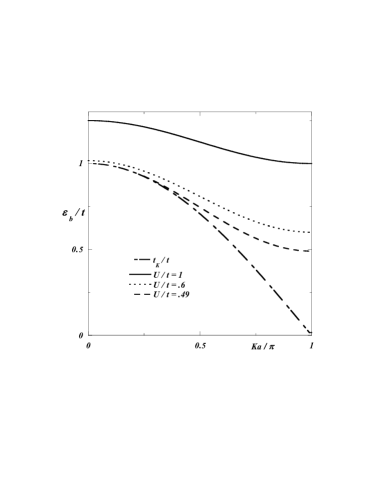
Figure 1: Dispersion curves of $t_{K}$ as a dashed-dotted line and of $\varepsilon_{b}(K)$ as solid, dashed and dotted lines, associated with various $U$ values, respectively; those data have been obtained with $t_{K}=t\cos\left(Ka/2\right)$, where $t,a$ are the one-electron bandwidth and the lattice parameter, respectively.

The $T_{c}$ dependence on $c_{0}$ will be discussed by assigning to $\rho(\epsilon)$ the expression, valid for free electrons

$$\rho(\epsilon)=\eta\sqrt{\epsilon-\epsilon_{b}}\Rightarrow c_{0}=\frac{2}{3}\eta\left(E_{F}\left(0,c_{0}\right)-\epsilon_{b}\right)^{\frac{3}{2}}\quad,$$ (7)

with $\eta=\frac{\sqrt{2}m^{\frac{3}{2}}V}{\pi^{2}\hbar^{3}}$, whereas $\epsilon_{b},m,V=17\AA^{3}$ stand for the bottom of the conduction band, electron mass and volume of the unit-cell, respectively. With help of Eq.(4), Eqs.(2,3) can be recast into a system of two equations

$$\begin{array}[]{l}E_{F}(0,c_{0})-\frac{\rho^{\prime}}{\rho}\frac{\left(\pi k_{B}T_{c}\right)^{2}}{6}-\frac{\varepsilon_{b}(K)}{2}=0\\ \left(\rho+\rho^{\prime\prime}\frac{\left(\pi k_{B}T_{c}\right)^{2}}{6}\right)^{-1}+\frac{\partial\mu}{\partial c_{s}}(K,c_{s}=0)=0\end{array}\quad,$$ (8)

to be solved for the two unknowns $c_{0}(T_{c}),t_{K}(T_{c})$ with $T_{c}$ being dealt with as a disposable parameter.

To that end, starting values are assigned to $U,t_{K}$, which gives access to $\varepsilon_{b}(K),\frac{\partial\mu}{\partial c_{s}}(K,c_{s}=0)$) and thence to $E_{F}\left(0,c_{0}\right),\epsilon_{b}$ and finally to $c_{0}$, owing to Eqs.(2,3,7). Those values of $c_{0},t_{K}$ are then fed into Eqs.(8) to launch a Newton procedure, yielding the solutions $c_{0}(T_{c}),t_{K}(T_{c})$. The results are presented in table 1. Since we intend to apply this analysis to high-$T_{c}$ compoundsarm , we have focused upon low concentrations $c_{0}<0.2$, which entails, in view of Eqs.(4,7), that $\left|\frac{\partial\mu}{\partial c_{s}}\right|$ takes a high value. This requires in turn $\varepsilon_{b}(K)\rightarrow t_{K}$ (see Eq.(6)) and thencesz5 $U\rightarrow\frac{t_{K}}{2}$, in agreement with $\frac{t_{K}}{U}\approx 2$ in table 1.

A remarkable property of the data in table 1 is that $c_{0},t_{K}$ are barely sensitive to large variations of $T_{c}$, i.e. $\left|\delta c_{0}\right|<10^{-3},\left|\delta t_{K}\right|<10^{-5}$ for $\delta T_{c}\approx 400K$. This can be understood as follows : taking advantage of Eqs.(2,4,7) results into

$$\frac{2E_{F}(0,c_{0})}{\varepsilon_{b}(K)}-1=\frac{\pi^{2}}{12}\left(\frac{k_{B}T_{c}}{\Delta(T_{c})}\right)^{2}\quad,$$

which, due to $\frac{dt_{K}}{dT_{c}}\approx 0,\Delta(T_{c})\approx 1eV,T_{c}=400K$, yields indeed $\delta c_{0}=c_{0}(400K)-c_{0}(1K)\approx 10^{-3}$, in agreement with the data in table 1. Such a result is significant in two respects, regarding high-$T_{c}$ compounds, for which $c_{0}$ can be varied over a wide range :

• because of $\frac{dc_{0}}{dT_{c}}\approx 0$, the one-electron band structure can be regarded safely as $c_{0}$ independent, which enhances the usefulness of the above analysis;

• the large doping rate up to $\approx 0.2$ is likely to give rise to local fluctuations of $c_{0}$, which, in view of the utmost sensitivity of $T_{c}$ with respect to $c_{0}$, will result into a heterogeneous sample, consisting in domains, displaying $T_{c}$ varying from $0$ up to a few hundreds of $K$. Thus the observed $T_{c}$ turns out to be the upper bound of a broad distribution of $T_{c}$ values, associated with superconducting regions, the set of which makes up a percolation path throughout the sample. However, if the daunting challenge of making samples, wherein local $c_{0}$ fluctuations would be kept well below $10^{-4}$, could be overcome, this might pave the way to superconductivity at room temperature.

Table 1: Solutions $c_{0}(T_{c}),t_{K}(T_{c}),\Delta(T_{c})$ ($\Delta(T_{c})=E_{F}\left(0,c_{0}(T_{c})\right)-\epsilon_{b}$) of Eqs.(8); $t_{K},\Delta,U$ are expressed in $eV$, whereas the unit for $c_{0}$ is the number of conduction electrons per atomic site.

$T_{c}(K)$	$c_{0}$	$t_{K}$	$\Delta$
$1$	$0.10215$	$6$	$1.1976$
$400$	$0.10225$	$5.9999$	$1.1984$

$U=3.39$ $T_{c}(K)$ $c_{0}$ $t_{K}$ $\Delta$ $1$ $0.14897$ $2$ $1.5402$ $400$ $0.14906$ $1.9999$ $1.5407$  $U=1.04$ $T_{c}(K)$ $c_{0}$ $t_{K}$ $\Delta$ $1$ $0.19158$ $4$ $1.8214$ $400$ $0.19167$ $3.9999$ $1.8219$  $U=2.2$

The $T_{c}$ dependence upon $U$ will be analysed with

$$\rho(\epsilon)=\frac{4}{\pi t}\sqrt{1-\left(1-\frac{\epsilon}{t}\right)^{2}}\quad,$$

where $2t$ stands for the one-electron bandwidth. Our purpose is to determine the unknowns $t_{K}(E_{F},T_{c}),U(E_{F},T_{c})$ with $E_{F}=E_{F}(T=0,c_{0})$ and $c_{0}=\int_{0}^{E_{F}}\rho(\epsilon)d\epsilon$. To that end, Eq.(3) will first be solved for $t_{K}$ by replacing $\frac{\partial E_{F}}{\partial c_{n}}(T_{c},c_{0}),\frac{\partial\mu}{\partial c_{s}}(0)$ by their expressions given by Eqs.(4,6), while taking advantage of Eq.(2). Then the obtained $t_{K}$ value is fed into Eq.(5) to determine $U$. The results are presented in Fig.22.

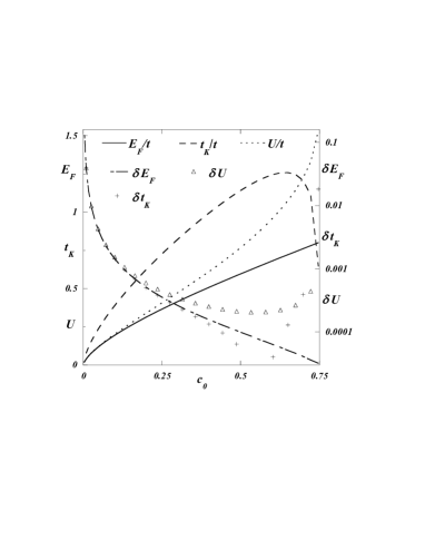
Figure 2: Plots of $E_{F}(T_{c},c_{0}),t_{K}(T_{c},c_{0}),U(T_{c},c_{0})$ calculated for $T_{c}=1K$ and $t=3eV$; the unit for $c_{0}$ is the number of conduction electrons per atomic site; $\delta f$ with $f=E_{F},t_{K},U$ is defined as $\delta f=\left|1-\frac{f(300K,c_{0})}{f(1K,c_{0})}\right|$; the scale is linear for $E_{F},t_{K},U$ but logarithmic for $\delta E_{F},\delta t_{K},\delta U$.

It can be noticed that there is no solution for $c_{0}>.75$, because $\frac{\partial E_{F}}{\partial c_{n}}(T_{c},c_{0})\approx\frac{1}{\rho}\left(E_{F}(0,c_{0})\right)$ and $\frac{\partial\mu}{\partial c_{s}}(0)>\frac{U}{2}$ decrease and increase, respectively, with increasing $c_{0}$, so that Eq.(3) can no longer be fulfilled eventually. But the most significant feature is that $\delta U$ is almost insensitive to large $T_{c}$ variation, except for $E_{F}\rightarrow 0$, i.e. for $E_{F}$ close to the Van Hove singularity, located at the bottom of the band, which has two consequences :

• $c_{0}$ cannot be varied in most superconducting materials, apart from high-$T_{c}$ compounds, so that $U$ is unlikely to be equal to $U(c_{0})$, indicated in Fig.22. Conversely, since high-$T_{c}$ compounds allow for wide $c_{0}$ variation, $c_{0}$ can be tuned so that $U=U(c_{0})$;

• the only possibility for a non high-$T_{c}$ material to turn superconducting is then offered at the bottom of the band, because $\delta U$ becomes large due to $\frac{\rho^{\prime}}{\rho}(E_{F}\rightarrow 0)\propto\frac{1}{E_{F}}$ in Eq.(4). Such a conclusion, that superconductivity was likely to occur in the vicinity of a Van Hove singularity in low-$T_{c}$ materials, had already been drawnsz5 independently, based on magnetostriction data.

It will be shown now that $\rho(\epsilon),\rho_{K}(\varepsilon)$ cannot stem from the same one-electron band. The proof is by contradiction. As a matter of fact $\rho(\epsilon)$ should read in that case

$$\rho(\epsilon)=\frac{4}{\pi t}\sqrt{1-\left(\frac{\epsilon}{t}\right)^{2}}\quad.$$

Hence $U>0$ entails, in view of Fig.11 and Eq.(2), that there is $\frac{\varepsilon_{b}}{2}=E_{F}>0$, which implies $\rho^{\prime}(E_{F})<0$ in contradiction with Eq.(3). Accordingly, since the two different one-electron bands, defining respectively $\rho(\epsilon),\rho_{K}(\varepsilon)$, display a sizeable overlap, they should in addition belong to different symmetry classes of the crystal point group, so that superconductivity cannot be observed if there are only $s$-like electrons at $E_{F}$ or if the point group reduces to identity. Noteworthy is that those conclusions had already been drawn empiricallymat .

The critical temperature $T_{c}$ has been calculated for conduction electrons, coupled via a repulsive force, within a model based on conditions, expressed in Eqs.(2,3). Superconductivity occurring in conventional materials has been shown to require $E_{F}(T_{c})$ being located near a Van Hove singularity, whereas a practical route towards still higher $T_{c}$ values has been delineated in high-$T_{c}$ compounds, provided the upper bound of local $c_{0}$ fluctuations can be kept very low. The thermodynamical criterions in Eqs.(2,3) unveil the close interplay between independent and bound electrons in giving rise to superconductivity. At last, it should be noted that Eqs.(2,3) could be applied as well to any second order transition, involving only conduction electrons, such as ferromagnetism or antiferromagnetism.