Network Hawkes Process Models for Exploring
Latent Hierarchy in Social Animal Interactions

Abstract

Group-based social dominance hierarchies are of essential interest in understanding social structure (DeDeo and Hobson,, 2021). Recent animal behavior research studies can record aggressive interactions observed over time. Models that can explore the underlying hierarchy from the observed temporal dynamics in behaviors are therefore crucial. Traditional ranking methods aggregate interactions across time into win/loss counts, equalizing dynamic interactions with the underlying hierarchy. Although these models have gleaned important behavioral insights from such data, they are limited in addressing many important questions that remain unresolved. In this paper, we take advantage of the observed interactions’ timestamps, proposing a series of network point process models with latent ranks. We carefully design these models to incorporate important theories on animal behavior that account for dynamic patterns observed in the interaction data, including the winner effect, bursting and pair-flip phenomena. Through iteratively constructing and evaluating these models we arrive at the final cohort Markov-Modulated Hawkes process (C-MMHP), which best characterizes all aforementioned patterns observed in interaction data.

As such, inference on our model components can be readily interpreted in terms of theories on animal behaviors. The probabilistic nature of our model allows us to estimate the uncertainty in our ranking. In particular, our model is able to provide insights into the distribution of power within the hierarchy which forms and the strength of the established hierarchy. We compare all models using simulated and real data. Using statistically developed diagnostic perspectives, we demonstrate that the C-MMHP model outperforms other methods, capturing relevant latent ranking structures that lead to meaningful predictions for real data.

1 Introduction

In this paper we consider the problem of providing a general model-based framework for exploring the unobserved social hierarchy among a group of mice through their observed repeated aggressive interactions. We do this using data from the study conducted by Williamson et al., (2016), in order to address unsolved questions in that work. In particular, describing the dominance structure behind such interactions well is a difficult task, and existing methods cannot adequately capture all possible dynamics, quantify uncertainty in the ranking, or provide insights into how a power hierarchy is formed or the distribution of that hierarchy.

There is no existing method which can describe how the observed interactions are generated from the underlying social hierarchy. Similarly, how mice are able to recognize their social status relative to other mice and how this recognition facilitates hierarchy formation and maintenance remains an unanswered question. The temporal dynamics in these interactions are driven by the need of the mice to explore, recognize, maintain, and exploit their positions in such a hierarchy, through mechanisms that are not fully understood. Section 2 presents an overview of existing well-known methods for dominance ranking and their properties. These existing methods, which generally utilise aggregate data, suffer several common issues, including the inability to rigorously evaluate the estimated ranking and the inability to deal with the temporal component of these interactions, which is likely influenced by the animals’ gains of social information about their group’s structure (Hobson et al.,, 2021). Specifying statistical generative models therefore provides a natural way to characterize the structure of these social groups more generally. One focus of the models we develop here is the ability to capture the latent stable dominance hierarchy via modeling the temporal and network dynamics of these social interactions. In Section 3, we take advantage of the timestamps of these interactions and propose three network point process models: the cohort Hawkes process model (C-HP), the cohort degree-corrected Hawkes process model (C-DCHP) and the cohort Markov-modulated Hawkes process model (C-MMHP). We construct these models such that these point processes are a function of a set of latent rank variables. These latent rank variables are a powerful feature of our models, allowing us to incorporate various known traits of animal behaviors in a social hierarchy into our model. We develop these models in a Bayesian framework to capture uncertainty estimates and to better model pairs which contain few interactions. We iteratively develop each model from the previous to better account for dynamics seen in animal data. This results in our final Cohort Markov-Modulated Hawkes Process (C-MMHP) model. In Section 4, these models are compared, using simulated and real data, to existing methods for understanding animal dominance ranking, highlighting how different methods capture different behavior components, leading to different rank estimates. We illustrate that our final model is flexible and adequately captures dynamics driven by the group’s inherent dominance hierarchy by showing results on rank inference, prediction performance and residual analysis. These point process models, therefore, provide a new utility for future research that can lead to better understandings of the dominance hierarchies among animals and be used to generate further research questions. Section 5 summarizes this work and discuss future directions for our proposed model.

2 Background

Here we review the literature on social hierarchy for group-living animals. Empirical studies of the social hierarchy of animals that live in a group are generally developed based on the observations of dyadic, or pairwise, agonistic interactions. In Williamson et al., (2016), the agonistic interactions include fighting, chasing and mounting behaviors. We consider all such aggressive interactions without differentiating the type, as is often done in this area (Lee et al.,, 2019). We denote the interactions between $N$ animals as a matrix $W$, where $W_{ij}$ is the number of aggressive interactions won by animal $i$ against animal $j$. In So et al., (2015) and Williamson et al., (2016), this is also called a win/loss matrix.

Two approaches are generally considered in the animal behavior literature to analyse this win/loss matrix (Drews,, 1993): functional methods and structural methods. Functional methods aim to directly infer a ranking of animals from this win/loss matrix by rearranging this matrix in an attempt to best capture behavioral patterns, expected in a social hierarchy. The rank is therefore inferred directly from the observations recorded in the win/loss matrix. If $W_{ij}>W_{ji}$ then functional methods infer that $i$ dominates $j$. Alternatively, structural methods propose an indirect model-based approach, associating a latent ranking variable $F_{i}$ with individual $i$. If $F_{i}>F_{j}$ then these structural methods infer that $i$ dominates $j$. These latent variables are constructed to satisfy a set of a priori assumptions, and structural models attempt to estimate these latent ranks to best align with the behavior captured in $W$.

An important concept in dominance ranking is linearity. Under a strict linearity assumption, for any three individuals, $i,j$, and $k$, if $i$ dominates $j$ and $j$ dominates $k$, then $i$ is assumed to dominate $k$. In social network research, this closed triad relationship is also called transitivity. For functional methods, the linearity assumption intuitively follows from observational studies of group-living animals. However, phenomena that violate a strict linearity assumption are often observed. In these cases, functional methods aim to find a nearly linear ranking that is most consistent with the observed wins and losses. Meanwhile, in structural methods, the linearity assumption is not directly observable but is incorporated as a property of the latent parameter $F$. The goal for structural methods is to study the model that can mostly reflect the potential formation mechanisms of dominance hierarchy.

One popular functional model is the I&SI method of de Vries, (1998). The I&SI method is a matrix-reordering method that identifies ordinal rankings of individuals that are most consistent with a linear hierarchy, by iteratively minimizing two criteria: the number of inconsistencies (I) and then, conditionally, the total strength of the inconsistencies (SI) without increasing I. The number of inconsistencies (I) is the number of pairs in which the lower-ranked individual wins more frequently than the higher-ranked individual in a given win/loss matrix, $\tilde{W}$,

$$I=\sum_{i>j}\mathbbm{1}_{\{\tilde{W}_{ij}>\tilde{W}_{ji}\}},$$

where $\mathbbm{1}_{\{\cdot\}}$ is an indicator function. The matrix $\tilde{W}$ is generated by reordering the original win/loss matrix $W$ according to a ranking of the individuals. The strength of a single inconsistency is the absolute rank difference of the inconsistent pair. Then, the total strength of the inconsistencies (SI) is the sum of strengths of all inconsistencies in $\tilde{W}$,

$$SI=\sum_{i>j}|i-j|\mathbbm{1}_{\{\tilde{W}_{ij}>\tilde{W}_{ji}\}}.$$

An example is shown in Figure 1. The original win/loss matrix in the example is $W$, which corresponds to $I=3$ and $SI=7$. According to the I&SI ranking method, the matrix is reordered to yield $\tilde{W}$, the rightmost matrix in Figure 1, in which $I=1$ and $SI=3$. Intuitively, the I&SI method finds the order of the rankings that is most consistent with a linear hierarchy. Although such a perfect linear hierarchy usually does not exist, I&SI aims to find a ranking where any inconsistencies take place between individuals that are close in rank. In other words, the I&SI method is most likely to allow for inconsistent dyads near the diagonal.

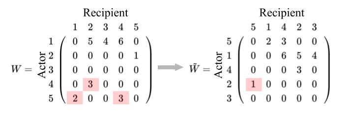
Figure 1: An example of a win/loss matrix and the corresponding reordered matrix according to the I&SI method. The entries shaded in red in the matrix are the inconsistencies, where the lower-ranked individual wins more frequently than the higher-ranked individual.

This method suffers from the problem that the algorithm is not guaranteed to converge to a unique optimal solution (de Vries and Appleby,, 2000). In particular, when there is a tie in the number of wins/losses ($W_{ij}=W_{ji}>0$) or an unknown relationship (i.e., where there is little information, $W_{ij}=W_{ji}=0$), the result highly depends on the choice of rules for assigning rankings. Another reason for the divergence is the method’s reliance on only an asymmetric relationship between the number of wins and losses, instead of the absolute difference. Such a simplified binary dominance measure ignores important information in the data – the total number of fights. It is often observed that the distribution of dominance power exhibits a high discrepancy (Chase et al.,, 2002), such as when highly ranked animals win a larger number of fights against intermediately ranked animals than these intermediate animals win against lowly ranked animals. This is seen in a win/loss matrix with large variation in the values of $W_{ij}$, but an ordinal ranking from a binary dominance measure is not discriminative enough to demonstrate that. Williamson et al., (2016) provide an analysis of monopolization of the most dominant mouse in each cohort, which suggests the necessity for considering a real-valued score instead of the ordinal rank.

Winner-loser models are an important family of structural methods that aim to explain the formation of linear dominance hierarchy (Lindquist and Chase,, 2009). Commonly, the models assume an innate power parameter for each individual $i$, denoted as $F_{i}$ (some models may assume a time-variant version, i.e. $F_{i}(t)$) (Bonabeau et al.,, 1999; Dugatkin,, 1997; Hemelrijk,, 2000). Although different models have their own specific formulations, common components they share are: an interaction probability and a dominance probability. Both are functions of innate power. The mathematical formulation of the models will not be discussed here, but some assumptions used in these model are of interest. One essential idea is the winner effect, the phenomenon in which an animal that has experienced previous wins will continue to win future aggressive interactions with increased probability. Although the extent and effectiveness of these winner effects remains unclear, evidence from experiments show that they exist and vary in different groups and species (Dugatkin,, 1997; Dugatkin and Earley,, 2003; Hsu and Wolf,, 1999). Experimental evidence also shows patterns that are challenging to capture through winner-loser models, such as bursting and pair-flips. Bursting means that higher-rank animals often exhibit successive fighting of lower-rank ones in an extended period of time. Pair-flips describe the situation when a pair of animals exchange the direction of their aggressive acts before a stable dominance relationship is established. A potential model for learning a latent hierarchy should therefore be able to incorporate these characteristics. In Section 4 we describe several existing structural and functional models in detail, which we use for comparison with our proposed methods.

2.1 Issues with conventional approaches

In summary, although the current methods have led to important insights on social structures among animals (So et al.,, 2015; Williamson et al.,, 2016; Hobson et al.,, 2021), they suffer from several issues that prevent them from being of utility for today’s increasingly available data with temporal information.

For functional methods, the use of an ordinal ranking alone may not be informative enough to describe the unequal distribution of dominance power which is commonly observed. The observed win/loss matrices are a noisy realisation of the true underlying dominance ranking among animals. Algorithms that attempt to directly derive the ranking by rearranging $W$ can therefore be unstable and unable to account for even small deviations from expected behavior. In addition, uncertainty measures are not available for the dominance ranking produced.

Structural models for such data provide much potential to understand the underlying drivers of animal behavior. However, methods to evaluate these models have been limited, as seen in Lindquist and Chase, (2009). These models are generally not built under the statistical framework of generative models. They fall short of providing a probabilistic connection between the observed social interaction timestamps and the underlying dominance hierarchies, and as such are unsuited to rationalize noisy patterns against the subject-matter assumptions of these models. As a result, a more systematic solution is needed for modeling the temporal dynamics of the dominance hierarchy, instead of relying on empirical scores. The timestamps of interactions among a group contain information about how the particular hierarchy formation and social information of this hierarchy are associated with social interaction patterns over time. This framework can provide better insights into the questions of Williamson et al., (2016) such as agnostic interactions in uncommon directions. The utilisation of a probabilistic generative model for latent ranking further provides the potential to rigorously assess model fit and help formalise scientific hypotheses. In the next section we will develop generative point process network models for this data, which we then compare with these existing methods in Section 4.

3 Latent ranking structured network point process models

In this section, we propose a series of probabilistic generative models to address common issues with conventional approaches, as discussed in the previous section. Inspired by theories on social hierarchy among group-living animals, there are various properties that we want to take into account when constructing these models: inconsistencies lying between the interactions and rankings, the time-evolving nature of the interaction dynamic, the winner effect, bursting and pair-flips phenomenons. For modeling the observed timestamps of social interactions, our models address three contributing mechanisms: the unobserved social hierarchy, the developmental influence from the animals’ social information about the social hierarchy, and temporal dependence on historical interactions.

We first introduce the required notation of point process models and network data, leading to a model for network point processes (Section 3.1). We then propose three such network point process models based on latent (structural) rankings (Section 3.2). We motivate the development of each of these models in turn by examining the properties each model fails to capture in one cohort of mice interaction data (described in Section 4.4), using the inference procedure described in Section 4.2.

3.1 Network point process models for animal interactions

Animal aggressive interaction data is essentially network data, where the senders are the winners of the fights and the receivers are the losers. To consider the necessary information lying in the timestamps of interactions, we introduce point process models on networks. In this section, we start with notation and a discussion on point processes in general (i.e., for non-network data), with a focus on the Hawkes process. We then introduce the notation for network event arrival data and network point process models.

Point process models.

Consider event arrival time data that consists of all event history up to a final-observation time $T$: $\mathcal{H}(T)=\{t_{m}\}_{m=0}^{M}$, where $t_{0}=0$, $t_{M}=T$, and $M$ is the total number of events. An equivalent representation of this event history $\mathcal{H}(T)$ is via a counting process, $N(t)$, where $N(t)$ is a right-continuous function that records the number of events observed during the interval $(0,t]$. The associated stochastic property is usually specified by its conditional intensity function $\lambda(t|\mathcal{H}(t))$ at any time $t\in(0,T]$, conditioning on current history $\mathcal{H}(t)$,

$$\lambda(t|\mathcal{H}(t))=\lim_{\Delta t\to 0}\frac{Pr(N(t+\Delta t)-N(t)=1|\mathcal{H}(t))}{\Delta t}.$$

This is the instantaneous expected rate of events occurring around a time $t$ given the history. Inference on the intensity function is conducted by evaluating the likelihood function for a sequence of events up to time $T$, $\mathcal{H}(T)$, which can be expressed as (Daley and Jones,, 2003)

$$\prod_{m=1}^{M}\lambda(t_{m}|\mathcal{H}(t_{m}))\exp\Big{\{}-\int_{0}^{T}\lambda(s|\mathcal{H}(s))ds\Big{\}}.$$ (1)

A Hawkes process (Hawkes,, 1971) is a linear self-exciting process that can explain bursty patterns in event dynamics. For a univariate model, the intensity function with exponential triggering function is defined as

$$\lambda(t)=\lambda_{1}+\sum_{t_{m}<t}\alpha e^{-\beta(t-t_{m})},$$ (2)

where $\lambda_{1}>0$ specifies the baseline intensity, $\alpha>0$ calibrates the instantaneous boost to the event intensity at each arrival of an event, and $\beta>0$ controls the decay of past events’ influence over time.

Network point process models.

Consider a network consisting of a fixed set of $N$ nodes, $V=\{1,2,...,N\}$. For each directed pair of nodes $(i,j)$, the observations of interactions (fights) between them up to terminal time $T$ includes the sender (winner) $i$, the receiver (loser) $j$ and a sequence of event times $\mathcal{H}^{i,j}(T):=\{t_{m}^{i,j}\}_{m=0}^{M^{i,j}}$. Hence, a network Hawkes process model has a conditional intensity function for each pair $(i,j)$ at time $t$ given by $\lambda^{i,j}(t|\mathcal{H}^{i,j}(t))$. The likelihood of the interactions on the whole network is then

$$\prod_{i=1}^{N}\prod_{j\neq i}^{N}\prod_{m=1}^{M^{i,j}}\lambda^{i,j}(t^{i,j}_{m}|\mathcal{H}^{i,j}(t^{i,j}_{m}))\exp\Big{\{}-\int_{0}^{T}\lambda^{i,j}(s|\mathcal{H}^{i,j}(s))ds\Big{\}}.$$

3.2 Latent ranking structured models for network point processes

Motivated first by the winner effect reviewed in Section 2, we model the conditional intensity of directed winning interactions between a given node pair as a function of their event (winning) history. Although experimental observations cannot explicitly verify the extent or persistence of influence of historical events, the intensity formulation in the Hawkes process (2) can help us model this winner effect flexibly. In a Hawkes process, $\alpha$ describes the extent to which previous wins influence the tendency to engage in a new fight. $\beta$ represents the persistence – how fast this effect decays over time. A large $\beta$ means that the winner effect decays quickly and only the most recent wins influence the tendency to engage in aggressive interactions at the present time.

For a directed pair $(i,j)$, the Hawkes process intensity is

$$\lambda^{i,j}(t)=\lambda^{i,j}_{1}+\alpha^{i,j}\sum_{k}\exp{(-\beta^{i,j}(t-t_{k}^{i,j}))},$$

where $\lambda^{i,j}_{1},\alpha^{i,j}$ and $\beta^{i,j}$ are pair-wise parameters in the Hawkes process. For all pairs, we will introduce structure in these pair-wise parameters below by assuming a latent rank variable, $f_{i}\in[0,1],\ i=1,2,...,N$. This is similar to the latent characteristic concept used in the winner-loser models (Lindquist and Chase,, 2009) and the latent rank in the aggregate-ranking model (De Bacco et al.,, 2018) reviewed in Section 4.1.2. The latent rank variable essentially embeds each individual in a one-dimensional unobserved ranking space. We constrain the pair-wise intensity function by bounding the latent rank in order to avoid issues with model identifiability. This latent rank variable is a powerful feature of our model as it allows us to incorporate various model assumptions on how the latent dominance hierarchy and historical events (i.e., social information) influence social interaction dynamics by specifying particular forms of the parameters $\lambda^{i,j}_{1},\alpha^{i,j}$ and $\beta^{i,j}$ in the intensity function, as we will discuss in Section 3.2.1, 3.2.2 and 3.2.3.

3.2.1 Cohort Hawkes Process (C-HP) Model

In the first model, we assume a baseline intensity, $\lambda_{1}$, and that the rate of decay for historical events, $\beta$, is constant across pairs. We structure the impact of historical events on each pair as a function of the pair’s latent ranks $f_{i},f_{j}$ and parameters $\mathbf{\eta}$, i.e. $\alpha^{i,j}:=g_{\mathbf{\eta}}(f_{i},f_{j})$. Inspired by the inconsistency and strength of inconsistency concepts in the I&SI method, we expect that the function $g_{\mathbf{\eta}}(f_{i},f_{j})$ satisfies the following: (1) $g_{\mathbf{\eta}}(f_{i},f_{j})>g_{\mathbf{\eta}}(f_{j},f_{i})$ when $f_{i}>f_{j}$; (2) $g_{\mathbf{\eta}}(f_{i},f_{j})$ is a decreasing function of $|f_{i}-f_{j}|$ when $f_{i}-f_{j}<0$. Hence, we consider,

$$g_{\mathbf{\eta}}(f_{i},f_{j}):=\eta_{1}f_{i}f_{j}\exp{(-\eta_{2}|f_{i}-f_{j}|)}\mbox{logistic}(\eta_{3}(f_{i}-f_{j})),$$

where $\eta:=(\eta_{1},\eta_{2},\eta_{3})$.

Each component here is motivated by empirical evidence of observed behaviors seen in animal data. In particular, we describe each term in this excitation function in detail:

• $\eta_{1}f_{i}f_{j}$ encodes the overall tendency of animals to continue fighting as a function of the product of their latent rankings. This results in pairs of higher ranked individuals being more likely to continue fighting. For higher ranked animals there is added incentive to clearly establish their dominance over similarly ranked animals, hence more repeated interactions. Meanwhile, for a pair of lower ranked animals, there is often less incentive to move from (say) the lowest rank of the hierarchy to the second lowest. This behavior is observed empirically in mice, with the higher ranked animals being most active throughout. Modeling the excitation parameter with the product of latent rankings allows us to capture this variation across pairs.

• $\exp\left(-\eta_{2}|f_{i}-f_{j}|\right)$ captures important properties found in existing methods within our model. This component gives an excitation parameter of the Hawkes process that is a decreasing function of $|f_{i}-f_{j}|$ when $f_{i}<f_{j}$. With this condition, this means that a weaker animal is less likely to continue winning fights against a stronger animal, with the likelihood of these events decreasing as the discrepancy between their latent rankings increases. This is motivated by the strength of inconsistencies component of the I&SI method and agrees with observed behavior.

• $\mbox{logistic}\left(\eta_{3}(f_{i}-f_{j})\right)$ ensures that $g_{\eta}(f_{i},f_{j})>g_{\eta}(f_{j},f_{i})$ when $f_{i}>f_{j}$. This condition means that wins are more often from a dominant animal to a submissive one. Again, this aligns with the inconsistency concept of the I&SI method while being a property observed in real data.

Figure 2-(a) shows the contour plot of $g_{\mathbf{\eta}}(f_{i},f_{j})$, with $\eta_{1}=4.46,\eta_{2}=0.18$, and $\eta_{3}=1.46$, which are estimated values from real data analyzed in Section 4.4. Note that the $x$-axis in Figure 2-(a) is decreasing from left to right, in order to be consistent with the arrangement of a win/loss matrix, where the interactions between the most dominant pairs are displayed in the top left. We notice that the function takes higher values when $f_{i}>f_{j}$ (upper right triangle of Figure 2-(a)), compared to values when $f_{i}<f_{j}$ (lower left triangle of Figure 2-(a)). This ensures that winning interactions are directed more frequently from a dominant individual towards a submissive individual, mirroring the inconsistency concept in I&SI method. The contour plot also shows that the form of this function agrees with the idea of minimizing the total strength of the inconsistencies in the I&SI method: it has a smaller value when $f_{i}<f_{j}$ and $|f_{i}-f_{j}|$ is larger (moving from the diagonal to lower left triangle of Figure 2-(a)).

Now, the intensity in the C-HP model is

$$\lambda^{i,j}(t)=\lambda_{1}+g_{\mathbf{\eta}}(f_{i},f_{j})\sum_{k}\exp{(-\beta(t-t_{k}^{i,j}))}.$$

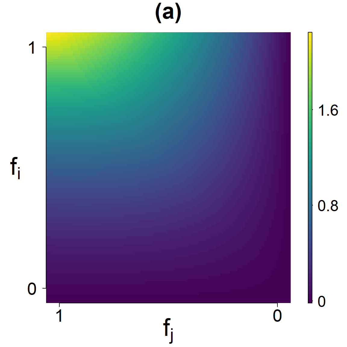
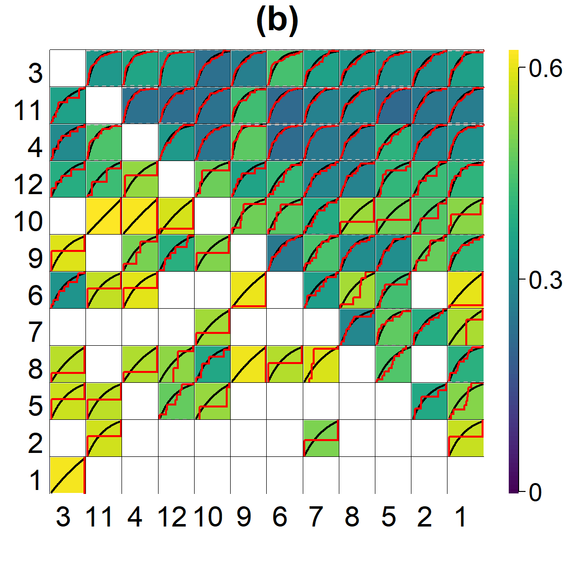
Figure 2: (a) Contour plot for $\alpha^{i,j}:=g_{\mathbf{\eta}}(f_{i},f_{j})$ where $f_{i},f_{j}\in[0,1]$. (b) Matrix of K-S statistics after fitting the C-HP model to the real data (reordered by I&SI ranking). The rows and columns of this matrix correspond to senders and receivers of an agonistic behavior, respectively. Color shading reflects the values of the K-S test statistics. Red lines are empirical cumulative distribution functions of rescaled-inter-event times and black lines are cumulative distribution functions of exponential random variable with rate 1.

To assess the goodness-of-fit of point process models, according to the time rescaling theorem (Brown et al.,, 2002), we can test whether the rescaled-inter-event times $\{\Lambda_{m}:=\int_{t_{m-1}}^{t_{m}}\lambda(s)ds\}_{m=1}^{M}$, are independently distributed following an exponential distribution with rate 1. We fit this model to data corresponding to interactions between a group of 12 mice, using the inference procedure of Section 4.2 We describe this data in more detail in Section 4.4. For each pair $(i,j)$, we conduct a Kolmogorov-Smirnov test on the rescaled-inter-event times $\{\Lambda^{i,j}_{m}:=\int_{t_{m-1}^{i,j}}^{t_{m}^{i,j}}\lambda^{i,j}(s)ds\}_{m=1}^{M^{i,j}}$ and show the test statistics result in Figure 2-(b). The background color indicates the value of the K-S statistics. This indicates good model fit for the C-HP model for the highly ranked animals (the top three rows of (Figure 2-(b)). The values of these K-S statistics increases, and there is evidence of a lack of fit as we move from the top rows of Figure 2-(b), particularly in the lower left diagonal. This is unsurprising as a majority of all interactions in this cohort are won by the 3rd animal (first row). As such, in the C-HP model, these interactions lead to a much larger value of $\lambda_{1}$ then would be suited to describe interactions between other nodes. This suggests that this model does not adequately address individual baseline event intensities when the number of interactions between pairs can vary widely. We introduce a correction to account for this next.

3.2.2 Cohort degree-corrected Hawkes process (C-DCHP)

The cohort Hawkes process model (C-HP) model assumes a constant baseline rate $\lambda_{1}$ and is incapable of modeling the degree heterogeneity of the observed nodes. However, it can be observed from Figure 2-(b) that this model tends to consistently fit poorly for pairs which include certain individuals, for example those pairs in which the sender (winner) is individual 10 or the receiver (loser) is individual 11. To address this issue, we extend the C-HP model, allowing varying baseline intensity rates across pairs. We accommodate degree heterogeneity in the pairwise baseline rate $\lambda_{1}^{i,j}$ by introducing a set of non-negative out-degree-correction parameters $\gamma_{i}$ and in-degree-correction parameters $\zeta_{j}$, $i,j=1,2,...,N$. With the baseline rate defined as $\lambda_{1}^{i,j}=\gamma_{i}+\zeta_{j}$, we have the intensity function as

$$\lambda^{i,j}(t)=\gamma_{i}+\zeta_{j}+g_{\eta}(f_{i},f_{j})\sum_{k}\exp{(-\beta(t-t_{k}^{i,j}))}.$$

This model introduces degree-correction parameters in the baseline rate of the C-HP model, hence, we refer to it as the cohort degree-corrected Hawkes process model (C-DCHP). Figure 3(a) shows the baseline intensity matrix after fitting this model to the same cohort in Figure 2-(b). These estimates suggest that a model which allows more flexible intensities may indeed be needed to capture the heterogeneity in behavior across individuals. We can see that this degree correction successfully adjusts for less active actors or recipients. For example, consider individuals $3$ and $6$; as shown in Figure 3, their estimated $\lambda_{1}^{ij}$s are relatively large indicating that both individuals are more active in terms of interaction frequency; individual 6 tends not to win many fights and individual 3 tends not to lose many fights. Importantly, these differences in activity level are individual-level attributes and require separate consideration when we are interested in learning about dominance hierarchy from dyad-level agonistic interaction data. The resulting inferred ranks from the C-DCHP model for such individuals are more consistent with the ranking obtained from existing methods, compared to the inferred ranks from the C-HP model. Similarly, to compare the fit of these models, we can look at the Pearson residuals (Wu et al., 2021a, ) from fitting each model to this data. We see, in Figure 3(b) that there is significant structure in the residuals after fitting the C-HP model, with large positive residuals for all interactions won by the top ranked animal. Fitting the C-DCHP model removes much of the structure in these residuals and better captures the heterogeneous nature of these pairwise interactions. However, the C-DCHP model consistently assigns a very large out-degree parameter value to the most dominant individual, as shown in Figure 3(a) and seen for all real data examples we consider. This complicates inference for the latent ranks of high-ranked individuals and leads to poor model performance for any interactions not involving this individual. In observed data, these interactions excluding this dominant individual more often exhibit more sporadic behaviour, with long periods where no events are observed, a feature we consider in the following model.

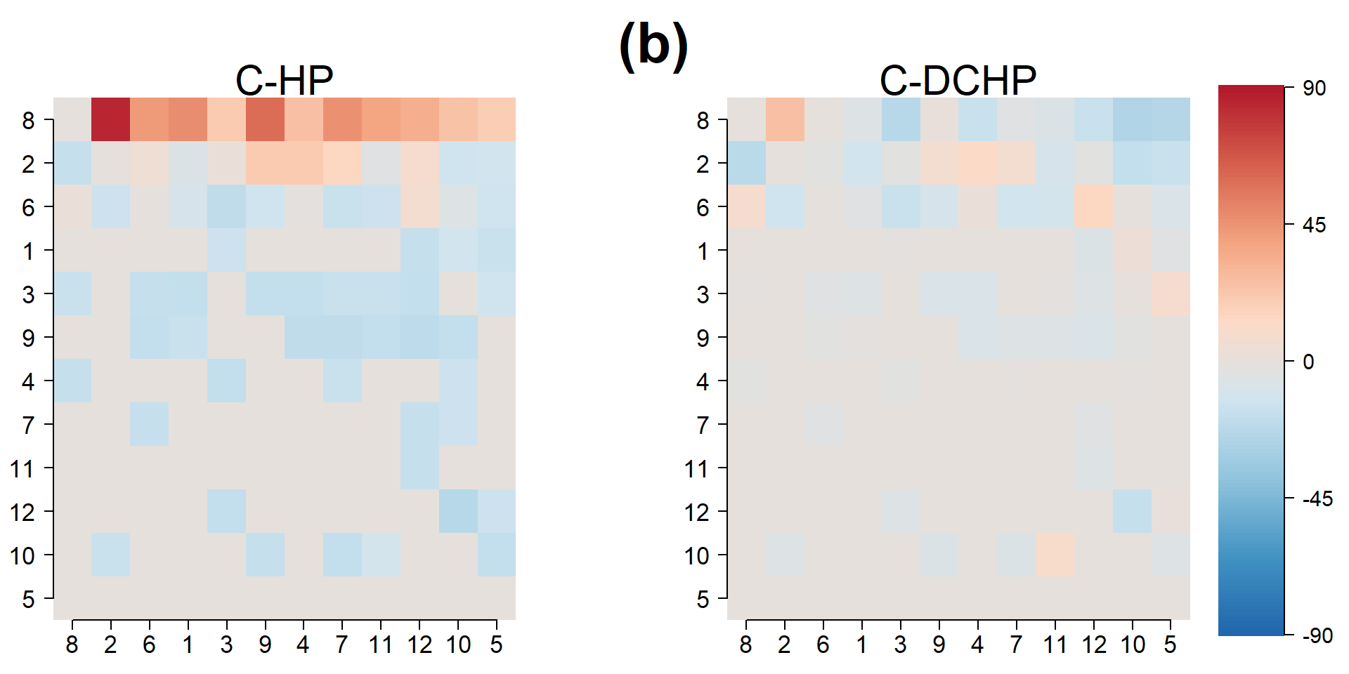
Figure 3: (a) Matrix of baseline rates $\lambda_{1}^{i,j}$ (reordered by I& SI rankings). These degree-corrected baseline rates allow for a more flexible node level model, clearly seen in the top row (a mouse which is involved in starting a large number of fights) and the bottom row (a mouse which does not start any fights but is often fought). (b) Pearson residuals for the C-HP and C-DCHP models.

3.2.3 Cohort Markov-modulated Hawkes Process (C-MMHP)

In Wu et al., 2021b , the Markov-modulated Hawkes Process (MMHP) is proposed to model general sequences of sporadic and bursty event occurrences. The model utilises a latent two-state continuous-time Markov chain (CTMC) $Z(t)$ to better describe event dynamics. In state 1 (the active state), events occur according to a Hawkes process, while in state 0 (the inactive state), according to a homogeneous Poisson process. The transition of $Z(t)$ is modeled through an infinitesimal generator matrix with parameters $\{q_{1},q_{0}\}$, with the first row corresponding to transitions from the active state, such that,

$$Q =\begin{bmatrix}-q_{1}&q_{1}\\ q_{0}&-q_{0}\end{bmatrix}.$$ (3)

Hence, for one MMHP, the conditional intensity function given the latent Markov process $Z(t)$, history events $\mathcal{H}(t)$ and parameter set $\Theta=\{\lambda_{0},\lambda_{1},\alpha,\beta,q_{1},q_{0}\}$ is

$$\lambda(t|Z(t),\mathcal{H}(t),\Theta)=\begin{cases}\lambda_{0},&\text{when }Z(t)=0,\\ \lambda_{1}+\alpha\sum_{k}\exp{(-\beta(t-t_{k}))},&\text{when }Z(t)=1.\end{cases}$$

Implicitly, the intensity function has the form

$$\lambda_{0}+(\lambda_{1}-\lambda_{0})Z(t)+\alpha Z(t)\sum_{k}\exp{(-\beta(t-t_{k}))}.$$

Thus, the latent process provides substantial flexibility in modeling the baseline rate as well as the extent of historical event influence.

We can readily extend this model to the network setting, where for directed wins between each pair $(i,j)$, the intensity follows,

$$\lambda(t|Z^{i,j}(t),\mathcal{H}^{i,j}(t),\Theta^{i,j})=\begin{cases}\lambda_{0}^{i,j},&\text{when }Z^{i,j}(t)=0,\\ \lambda_{1}^{i,j}+\alpha^{i,j}\sum_{k}\exp{(-\beta^{i,j}(t-t^{i,j}_{k}))},&\text{when }Z^{i,j}(t)=1.\end{cases}$$ (4)

Here $\Theta^{i,j}:=\{\lambda_{0}^{i,j},\lambda_{1}^{i,j},\alpha^{i,j},\beta^{i,j},q_{1}^{i,j},q_{0}^{i,j}\}$ is the parameter set for pair $(i,j)$. $q_{1}^{i,j}$ and $q_{0}^{i,j}$ are the instantaneous transition probabilities for the latent CTMC $Z^{i,j}(t)$ of a pair $(i,j)$. $Z^{i,j}(t)$ are independent across pairs. The transition probability $q_{1}^{i,j}$ ($q_{0}^{i,j}$) represents the probability that pair $(i,j)$ transitions out of the active (inactive) state and is modelled as a function of the latent ranks, $f_{i},f_{j}$. To understand the behavior of these latent state transition parameters for each pair $(i,j)$, consider the stationary distribution of the latent CTMC, $Z^{(i,j)}(t)$. For an irreducible and recurrent CTMC $Z(t)$ with infinitesimal generator as shown in (3), a stationary distribution $\pi$ satisfies $\pi^{T}Q=0$ (Yin and Zhang,, 2012). Hence for a pair $(i,j)$, the limiting behavior of their latent state transitions dictates that they spend $\frac{q_{0}^{i,j}}{q_{0}^{i,j}+q_{1}^{i,j}}$ of their time in the active state, and all remaining time in the inactive state. With the hope that if $i$ dominates $j$, i.e. $f_{i}>f_{j}$, the pair $(i,j)$ will spend lots of time in the active state, we form the transition probabilities as,

$$q_{1}^{i,j}=\exp{(-\eta_{3}f_{i})}$$

$$q_{0}^{i,j}=\exp{(-\eta_{3}f_{j})}.$$

Hence, when individual $i$ is stronger than individual $j$, node $i$ is more likely to start and continue winning against node $j$ (i.e. large $q_{0}^{i,j}$ and small $q_{1}^{i,j}$) than to observe wins from $j$ to $i$. This follows the asymmetry property of aggressive behavior in group animals. The limiting distribution of time spent in state $1$ is $\mbox{Logistic}(\eta_{3}(f_{i}-f_{j}))$.

Given the latent process between pair $(i,j)$, $Z^{i,j}(t)$, we assume that $\beta^{i,j}$ is a constant $\beta$ across pairs. In a similar vein to the C-HP and C-DCHP models, we model the winner effect $\alpha^{i,j}$ as taking the form $\eta_{1}f_{i}f_{j}\exp(-\eta_{2}|f_{i}-f_{j}|)$. The third component of the excitation parameter in these first two models is now replaced by the latent state indicator $Z^{i,j}(t)$. As such, this equips the conditional intensity in the C-MMHP model with additional flexibility, alternating between a simpler homogeneous Poisson process and a self exciting Hawkes process, with the limiting distribution of the process aligning with the C-DCHP model. Markov modulation allows the self-exciting component of the intensity to dissipate at points during the observation period, a phenomenon that is often observed in animal behavioral studies where interactions can be sparse at certain times. In other words, this modulation is introduced to account for the often seen sporadic nature of interactions between animals, arising from initial exploratory aggressive interactions and later interactions which may determine the precise hierarchy, before potentially stabilising.

Like the C-DCHP, we again consider the degree correction described in the previous model here, giving $\lambda_{0}^{i,j}=\gamma_{i}+\zeta_{j}$. $\lambda_{1}^{i,j}$ is defined by

$$\lambda_{1}^{i,j}=\lambda_{0}^{i,j}(1+w_{\lambda}),$$

for a common $w_{\lambda}\geq 0$, to ensure that the base rate of the point process in the active state is greater than the inactive state. Hence we have the intensity from $i$ to $j$ given by

$$\lambda^{i,j}(t)=\lambda_{0}^{i,j}+(\lambda_{1}^{i,j}-\lambda_{0}^{i,j})Z^{i,j}(t)+\eta_{1}f_{i}f_{j}\exp(-\eta_{2}|f_{i}-f_{j}|)Z^{i,j}(t)\sum_{k}\exp{(-\beta(t-t_{k}^{i,j}))}.$$

This proposed model therefore provides a potential mechanism to describe the establishment of a realised dominance structure, as an expression of a latent hierarchy, by incorporating each of the components of the C-DCHP model and allowing Markov modulation. This is a key step towards better understanding the true process behind such interactions, a key question highlighted by Williamson et al., (2016). The mechanism we propose here agrees with existing methods from the animal behavior literature and captures properties commonly seen in data of this form. For example, bursty behavior is commonly seen in aggressive and subordinate interactions (Lee et al.,, 2019), which is readily incorporated into our model through the use of a Hawkes process. Through the parameterization of the Hawkes process, our proposed model is also designed to capture a linear hierarchy. This agrees with many of the existing methods in this area. However, these existing aggregate methods fail to adequately account for wins in unexpected directions, such as from lower ranked to higher ranked animals, which can and do occur. Interactions such as these are unsurprising, particularly when the animals are first placed together, as they fight to gain social information about the social hierarchy. These interactions may continue to occur also. It can be advantageous for animals to improve their position by beating similarly ranked animals, to better obtain limited resources and potentially dissuade lower ranked animals from being aggressive towards them. While this is only seen among strong mice, in other species it occurs throughout the hierarchy (Hobson et al.,, 2021).

We observe this only among the top ranked mice in our data, where the top ranked animal can be defeated late in the observation period (Williamson et al.,, 2016). By equipping each directed interaction pair with a point process, there is always some likelihood that interactions will be observed between animals in an uncommon direction. Our C-MMHP model goes further than this. With a Markov Modulated Hawkes Process, we allow the likelihood for interactions to vary in time, alternating between a Poisson process and a Hawkes process. This additional flexibility is well suited for capturing interactions in an uncommon direction. In particular, interactions of this type are often sporadic, often occurring after long periods where there are no interactions between that pair or in that direction.

3.3 Model inference

Bayesian modeling.

Throughout this paper, we adopt a Bayesian framework for our model inference. Assuming a prior distribution for the model parameters and given a model likelihood, the posterior distribution for quantities of interest can help us calibrate the uncertainty in the model. This is an important aspect of our current research strategy. First, we need tools that can quantify uncertainty in rank inference. For example, in Williamson et al., (2016), the analysis shows that the pair-flips phenomenon exists in some cohorts, which means that the direction of aggressive interaction changed over time. In a Bayesian modeling framework, we can naturally capture this effect through uncertainty in the model parameters: we suspect that individuals that are involved in pair-flip phenomena should have larger posterior variances for their latent ranks. Second, in each cohort, there always exists some pairs that have few or no interactions across the observation time window. A Bayesian framework can achieve robust inference in such conditions, with the assistance of prior assumptions and by borrowing strength from the data of other pairs. In this paper, we will use the Stan modeling language (Carpenter et al.,, 2017) to fit all models and to obtain posteriors samples for model parameters. We describe further details of our inference procedure in Section 4.2.

4 Results

4.1 Comparison Models

Before analysing the performance of our models on both real and simulated data, we first describe in detail existing methods used to analyse dominance behavior in animals, which we shall use for comparison of inferred rankings. As described above, these methods can be broadly classified as functional and structural.

4.1.1 Functional methods

Along with the I&SI method, So et al., (2015) and Williamson et al., (2016) use the Glicko rating system to calculate temporal changes in dominance scores of each animal in each cohort. This is a dynamic paired comparison system that calculates a temporal sequence of cardinal scores based on the history of dyadic wins and losses (Glickman,, 1999). All individuals start with the same initial rating. After each observed fight between a pair, the winner (or the loser) gains (or loses) points according to a decreasing function of the difference between their previous scores. In this case, fighting between pairs whose scores differ a lot will not result in significant changes in the system. The calculation of the Glicko score depends on a predefined constant, which determines the volatility of the score changes. Since scores are computed after each fighting event, this method can capture the temporal dynamics of the dominance hierarchy, although it does not account for temporal components, such as the time between events. Williamson et al., (2016) also provides a clear visualization of the change in the dominance score based on this method, where the emergence and stabilization of the hierarchy can be easily deduced from the graph. However, this method is ad-hoc in the sense that there are no theoretical rules for researchers to choose important key aspects of this method, including the initial rating, the decreasing function for changing a pair’s scores after an observed fight, or the constant controlling the volatility of score changes. Since the method focuses on summarizing the observations without any formal modeling, it can be hard to provide formal insights regarding the evolution of hierarchy dynamics. It is also not always clear how to draw a conclusion about the hierarchy structure from the visualization of the rating system.

4.1.2 Structural methods

Lindquist and Chase, (2009) apply winner-loser models to real experimental data of hens and show the lack of fit between these models and the data. However, this procedure is qualitative only, by comparing simulation results from the models with the real data. The probabilistic generative models we proposed in Section 3 are able to capture these important animal behavior phenomena, including the winner effect, bursting and pair-flips. We also develop a corresponding statistical inference procedure which means that model-fitting can be assessed by rigorous statistical model diagnostics, rather than relying on simulations as in Lindquist and Chase, (2009). We analyse our models using these diagnostics in Section 4.3 and Section 4.4.

A more recent structural model is De Bacco et al., (2018), which introduced a physics-inspired model to infer cardinal hierarchical rankings of individuals in directed networks. By assuming that individuals are more likely to interact with others of similar rank, they propose an optimization solution and a generative model to find real-valued ranks of individuals. For a pair $(i,j)$, with latent rank variables $f_{i}$ and $f_{j}$, the aggregate-ranking model uses Poisson regression to model the aggregate counts between the pair over the entire observation period, denoted as $N_{i,j}$, as a function of the difference in their ranks. This is essentially the counting process evaluated at time $T$, $N^{i,j}(T)$, ignoring the exact event times. The only information used in the model is the existence and direction of the interactions in the network. We refer to this model as the aggregate-ranking model. Only using the aggregate counts of interactions makes it hard to address phenomena like the winner effect, bursting and pair-flips mentioned in Lindquist and Chase, (2009). Event time data which records when the aggressive behaviors occur is highly detailed and contains information needed to describe the important phenomena mentioned earlier.

4.2 Model implementation

To perform inference for each of these models we perform Bayesian inference using the Stan programming language (Stan Development Team,, 2020). We impose weakly informative priors for the model parameters where possible. In particular, for each model we use $\mbox{half-N}(0,1)$ priors on $\eta_{1},\eta_{2},\eta_{3}$ and $\beta$, $\mbox{U}[0,1]$ priors for $f$, and a $\mbox{half-N}(0,1)$ prior for $w_{\lambda}$ in the C-MMHP model, to ensure that the rate in the active state is greater than in the inactive state. For the degree-corrected models we place Laplace priors on $\gamma$ and $\zeta$, to account for nodes which do not win or lose any fights. Full details of the inference procedure to infer the latent states of the C-MMHP model are given in Wu et al., 2021b .

4.3 Synthetic results

We first wish to validate our proposed models using simulated data where we aim to recover the ground truth latent ranking vector. To compare the three proposed models, we simulate 50 independent C-MMHPs generating event winning times between 10 nodes with uniformly separated true latent ranks. By fitting the synthetic data with our proposed three models, we can obtain the inferred latent ranks as shown in Figure 4-(a). Inference using C-MMHP and the C-DCHP both recover the true latent ranks well, with the C-HP showing considerable bias for several nodes. It is unsurprising that there is little difference between the inferred rankings from the C-DCHP and C-MMHP model, given their similar limiting distribution. Figure 4-(b) shows an example of estimated intensity for one pair of individuals in one simulated process (from the top ranked to second ranked individual), indicating that the C-HP and C-DCHP models cannot capture the true intensity as well as the C-MMHP model. The C-HP incorrectly captures the true decay parameter while both the C-HP and C-DCHP model overestimate the intensity repeatedly for events which occurred in the inactive state, with both showing more over and underestimation, althought the C-MMHP does incorrectly classify some events.

We also compare the inferred ranking from each of these models and the comparison models discussed previously with the known true ranking. We summarize this using the Spearman rank correlation between the estimated ranking obtained from each method and the true ranking, as shown in Figure 5. We note that the C-MMHP model recovers the true ranking best, with the C-HP and C-DCHP models also performing well but showing more variability. As a structural method, the I&SI model recovers the true ranking reasonably well for simulations from the generative C-MMHP model. In this scenario a large proportion of fights occur in the active state of the simulated C-MMHP model and so agreement between the I&SI method and our proposed models is expected.

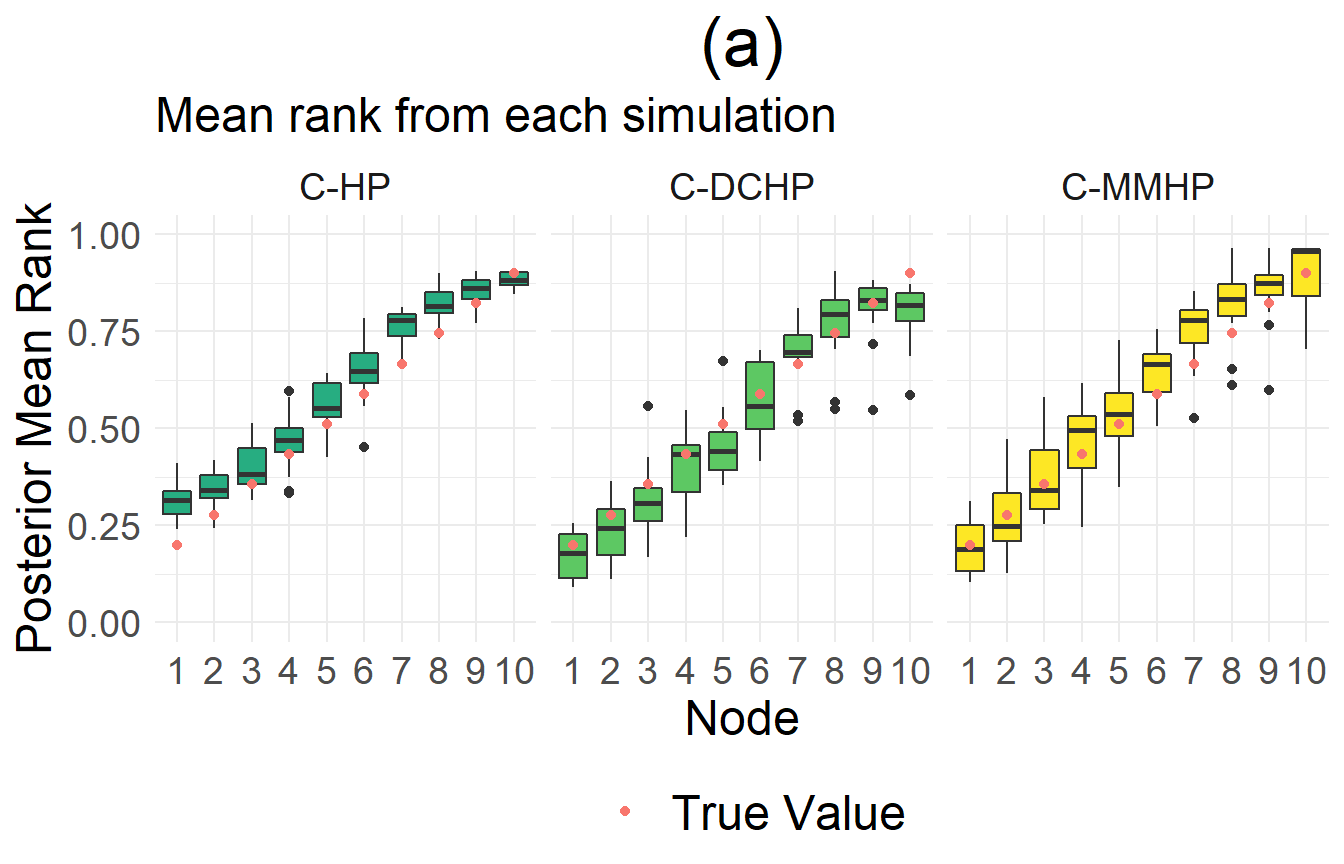
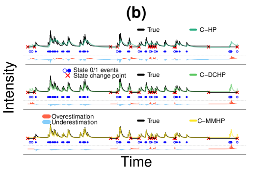
Figure 4: Simulation results from simulating 50 interaction datsets with common C-MMHP parameters. (a) Shows posterior inference of latent rank variable $f_{i},i=1,\dots,10$ by C-HP, C-DCHP and C-MMHP. Each value is the posterior mean for $f_{i}$ inferred from 50 independent simulations from a C-MMHP model with the same underlying parameters, with the true rank values overlaid in red. (b) Show the inferred intensity for one pair of individuals (top ranked to second highest ranked) in one simulation using three models. Here we fit each of the C-HP, C-DCHP and C-MMHP models to this data and plot the inferred intensity function for this pair. The events and the state they occurred in, along with the times the process changed state, are also shown in this plot. The red/blue shaded area underneath shows the magnitude of the error in the estimation of the intensity in terms of overestimation and underestimation.

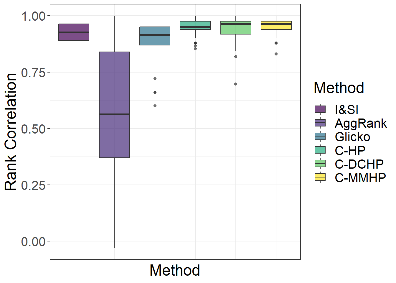
Figure 5: Shows the Spearman rank correlation between the inferred ranking from each of these models, along with existing methods, and the known true ranking.

4.4 Real data results

We next fit our models, C-HP, C-DCHP and C-MMHP to the ten mice cohorts studied by Williamson et al., (2016), which consisted of placing each cohort of twelve male mice in a large custom built vivarium. Intensive behavioral observations were conducted for one to three hours per day during the dark cycle over twenty-one consecutive days. Trained observers recorded all occurrences of the behaviors (including fighting, chasing, mounting, subordinate posture and induced-flee). The details of each behavioral event are also recorded, identifying the actor which wins the interaction and the actor which loses the interaction, along with the timestamp and location.

Using various measurements in social hierarchy analysis and social network analysis, Williamson et al., (2016) demonstrates that these mice cohorts form significantly linear social dominance hierarchies. The work also examines the temporal changes in the mice social hierarchy and shows that in most of the ten cohorts, the dominance hierarchies emerge rapidly and become stable by the end of the second week. Although results of the quantitative analysis are thoroughly discussed and the patterns in the temporal dynamics are summarized qualitatively, there are still observations in some cohorts that disagree with the authors’ speculations, which have been unexplained in existing work but are naturally accounted for in our model. We have addressed how our model provides a potential mechanism for the connection between the establishment of a latent ranking of these animals with the observed social interactions and described how it captures interactions in an uncommon direction. We will verify that our model does describe this data well using multiple metrics, illustrating that a flexible probabilistic model incorporating these hypothesised processes can be constructed. We then also show how further information may be available from these models, such as information about the distribution of individuals’ dominance power. We also compare the results from fitting the following existing models to this data: a dynamic social network in latent space model, and a Markov-modulated Hawkes process without incorporating any latent ranking structure between the nodes. We first briefly describe these models. Additional analysis results for each individual cohort are available in a supplemental file.

Dynamic social network in latent space model (DSNL)(Sarkar and Moore,, 2006).

This model is constructed for dynamic network data with binary links which is observed in discrete time steps. The model associates each node in the network with a latent space variable that can move in discrete time, and specifies that the move is Markovian. For node $i$ at discrete time $d$, the latent variable is denoted as $f^{(d)}_{i}$. We tailor this model to our observed mice interaction data by changing the binary link assumption in the original model to allow for aggregate counts by using a Poisson link instead of a logistic link. We construct discrete time steps to be the ending time of each day in the observation time window, i.e. $t^{(d)}$. Hence, for each pair $(i,j)$, we have the count of their interactions during day $d$, $N_{d}^{i,j}:=N^{i,j}(t^{(d)})-N^{i,j}(t^{(d-1)})$, where $N^{i,j}(t)$ is the counting process for pair $(i,j)$ evaluated at time $t$. Further details of this model will be omitted here.

Markov-modulated Hawkes process without network ranking structure (I-MMHP) (Wu et al., 2021b, ).

In this model, we assume that the intensity function of (4) allows for different parameter values $\Theta^{i,j}$ across pairs. This means there is no structure between nodes and a latent ranking of the animals cannot be inferred. The independent structure of the parameters in this model is less constrained than our C-MMHP model, where we consider network structure between nodes to learn latent rankings.

Summary measures for evaluating model performance.

Our real data analysis results will be summarized from several perspectives: (i) inference for the latent ranks and a summary of the properties captured by each of the different methods, prediction performance, both in terms of (ii) predicted events and (iii) predicted evolution of dynamics over time and (iv) additional insights available through the C-MMHP model, which may provide potential future research directions. We compare the results of the C-HP, C-DCHP and C-MMHP models under the first three of these perspectives. Because the nature of the three other comparison models - aggregate-ranking, DSNL and I-MMHP - differs, they are fitted and compared from different perspectives. The aggregate-ranking model (and also the I&SI method we discussed previously) estimates a static ranking and will be discussed in terms of inference for the latent ranks only. The I-MMHP is a point process model and can be evaluated using the same point process methods as our latent ranking point process models. However, the I-MMHP cannot be used to infer a latent ranking. Finally, both the DSNL and I-MMHP models can perform prediction of events (or event counts) and can serve as comparison models in the prediction performance section.

4.4.1 Inference on latent rank

We fit the C-HP, C-DCHP, C-MMHP and aggregate-ranking models to our data of ten cohorts separately. Figure 6 shows the relationship between I&SI rank and posterior draws of latent ranks using our three models and aggregate-ranking model in two cohorts, Cohort 5 in Figure 6 (a) and Cohort 3 in Figure 6 (b). While we have ordered the animals by their estimated I&SI ranking, this is not to take it as some reference ranking but to highlight how our models capture a different ranking structure. These cohorts display the two types of common characteristics we observe across the 10 cohorts. Cohort 5 provides an example of general behavior seen in 7 of the 10 cohorts studied here. In this example, there is general agreement between the rankings inferred from each of the Hawkes models, with the C-MMHP model displaying less uncertainty than the alternative models. The C-MMHP model identifies 3 approximate groups within the rankings, which is seen in several cohorts. As such, the bursty model assumption seems to agree with the dynamics evident here, with these bursty dynamics largely aligning with the power hierarchy. We also see animals such as # 7 and # 10 where the ranking from the C-MMHP model deviates from the I&SI ranking, as these animals are involved in relatively few fights and as such there are few periods of bursty fights. In this cohort all animals lose a similar number of fights, with the percentage of all fights which are classified as active by the Markov modulation being very high for the whole cohort.

Different from the seven cohorts represented by cohort 5, Cohort 3 and another two cohorts exhibit another form of common behavior. Here it is difficult to identify differences in the rankings for many of the animals. There is also weaker agreement between the C-MMHP model and the C-HP/C-DCHP models, while we also see disagreement between the I&SI ranking and the simplest of our models, the C-HP model. Interestingly, here all inactive originate from animal # 5, which is ranked significantly lower by the C-MMHP model than its I&SI ranking. Similarly, this animal has a large relative out degree estimate under both the C-DCHP and C-MMHP models. For these cohorts there are a large number of sporadic fights and a large percentage of wins attributed to a single animal, who seems to indiscriminately win fights against all other animals repeatedly. Although this behavior is rewarded by traditional ranking methods, it is not clear that this should be an indication of dominance, with other animals perhaps unable to learn social information about the losers of these fights (Hobson,, 2020). Our C-MMHP model places less emphasis on this behavior, giving such animals a lower ranking than existing methods.

Given that the Aggregate Ranking method and the I&SI method use the same win/loss matrix information, it is expected that they show strong agreement.

Figure 6: Real data fitting results. (a) Comparison of rank inference using different model with I&SI rank for Cohort 5. (b) Comparison of rank inference using different model with I&SI rank for Cohort 3.

4.4.2 Prediction

We can also use posterior predictive distributions to validate the models considered. For each model, we split the data into two time periods: (1) the first 15 days of data, $\mathcal{H}^{i,j}(t^{(15)})$, where $t^{(d)}$ is the ending observation time for the $d$-th day, which is used to estimate the model and (2) a prediction window from day 15 to day $t^{(d)}$, for $d=16,...,21$, the remaining observation period, which allows us to compare models across different prediction horizons. For each prediction horizon $t^{(d)}$, we generate a predicted point process separately over the time period $t^{(15)}$ to $t^{(d)}$, given each posterior draw of parameters and the historical events in the first 15 days. Hence, the predicted counting process $\hat{N}^{i,j}(t)$ is constructed by generating processes in each prediction period and adding these to the true process in the model-fitting period. For each prediction horizon and model, we generate 1000 posterior processes, corresponding to 1000 posterior draws from the posterior distribution for the model parameters. Following Sarkar and Moore, (2006), we can also make predictions over these same time windows using the DSNL model.

Two aspects of the predictions are evaluated, the accuracy of predictions for the interaction counts and the prediction of the rankings.

For each point process model and for each different prediction horizon $d=16,...,21$, the number of total interactions for pair $(i,j)$ during the prediction period can be estimated by $\bar{\hat{N}}^{(i,j)}(t^{(d)})-N^{(i,j)}(t^{(15)})$, where $\bar{\hat{N}}^{(i,j)}(t^{(d)})$ is the average count of wins across 1000 posterior processes. We arrange the prediction counts in a matrix $\hat{A}^{(d)}$ such that each $(i,j)$ entry is the predicted number of interactions for pair $(i,j)$ from the end of the 15th day until the $d$th day. To quantify the accuracy of these predicted counts, we use the mean absolute error (MAE) of the difference between the estimated and real win/loss matrix $A^{(d)}$,

$$\frac{1}{n}\sum_{i,j}|\hat{A}^{(d)}_{ij}-A^{(d)}_{ij}|$$

The smaller the MAE, the closer the model’s predictions of the interaction counts are to the observed data. Figure 7-(a) summarizes the result across all cohorts, by taking the median predicted counts for each pair across each of 1000 posterior draws. The C-MMHP, C-DCHP and I-MMHP models provide the best predictions of interaction counts, with the smallest MAE across all prediction horizons, with C-MMHP slightly outperforming the other models.

We also infer a proxy predicted rank of individual $i$ at prediction time $t^{(d)}$ by introducing the out-degree intensity

$$\hat{\lambda}_{i}(t^{(d)})=\sum_{j}\hat{\lambda}^{i,j}(t^{(d)}).$$

The Glicko score ranking system serves as a bench mark for us to compare to, as it is a dynamic score. While this is not a true dynamic score, we can construct it for each of the models we consider here, allowing us to use it as a comparison across them, identifying agreement between each of these models and the evolution of the Glicko ranking. We compute the Spearman rank correlation of our inferred rank with the Glicko score at the end of the prediction day. Figure 7-(b) summarizes the result for all cohorts. The C-MMHP model closely aligns with the Glciko score, with rank correlation close to 1, while the unconstrained I-MMHP model also performs well in this scenario.

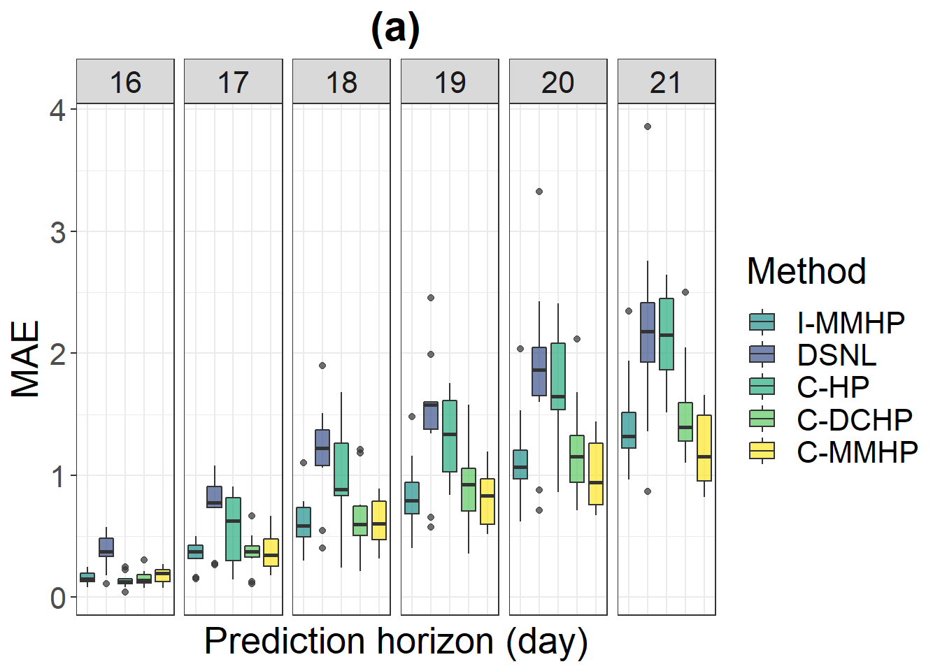
Figure 7: Prediction of events and rank. (a) shows the MAE of predicted error for all cohorts, using the median predicted count for each model for each cohort on each day. (b) Summarizes the Spearman rank correlation of predicted rank for all cohorts, where each cohort is predicted by the posterior mean of $\hat{\lambda}_{i}(t^{(d)})$.

Our posterior predictive processes can even be used to forecast the Glicko scores over future prediction windows, since we obtain the full event history from the generated process. In contrast, the DSNL model can only provide day-level predictions, which we have evaluated previously. Figure 8-(a) shows the prediction of Glicko scores over days 19-21 when fitting the data in the first 18 days to the C-MMHP model. Our prediction bands can forecast temporal trends of Glicko ratings in the real data and provide an appropriate representation of the uncertainty in these predictions, which we illustrate in Figure 8-(a). These prediction bands correctly separate the rankings of most animals, particularly the highly ranked nodes, and capture the groups of rankings that seem to have formed for this cohort. Being able to predict rank evolution over time is not possible using existing methods and this could be of use in the experimental design of these studies to guide data collection, such as the ability to isolate mice who would be expected to rank similarly in the original group.

4.4.3 Additional insights from the C-MMHP model

Finally, we wish to highlight some additional insights which are available after fitting our C-MMHP model. Since our C-MMHP model can separate wins into active and inactive states, such separation can serve as a prepossessing step for the data. To illustrate this, we first fit the C-MMHP model to the data for one cohort and classify the wins into active and inactive states according to the estimated latent Markov process. The two types of interactions can then be fitted separately using other animal behavior models. Wu et al., 2021b shows that the wins in the active state more closely follow a linear hierarchy, as compared to the set of all wins or the set of inactive wins; this provides an explanation for the pair-flips phenomenon. During the active state, pairs are engaging in aggressive interactions and actively trying to navigate the social hierarchy, while in the inactive state, the wins are more or less random and lack specifically directed aggression seen in the active state. As an example, we fit the DSNL model to the set of overall events, active events and inactive events separately, and calculate the Spearman rank correlation between the latent ranks for each day as estimated by the DSNL model and the Glicko ratings at the end of each day. Figure 8-(b) shows these rank correlations on each day for the three types of wins. This suggests that the information contained in these wins varies over time, with the inactive state showing a stronger correlation with the Glicko ranking in the start and middle of the observation period. Similarly, as Williamson et al., (2016) pointed out, the distribution of individual dominance power within animal groups is an important question. One way we can address this is by looking at the “out” degree estimates from our C-MMHP model. In particular, we see significant agreement between the out degree parameter estimates and whether Williamson et al., (2016) could identify the dominant animal after the first week. Where this animal could be clearly identified early on, the C-MMHP model resulted in a much larger out degree estimate for that animal than the rest of that cohort. This was not the case for the two cohorts where the dominant animal took longer to establish itself. This out degree parameter may therefore provide some insights into the distribution of individual dominance power within a given group, although further work is needed to further investigate this important question posed by Williamson et al., (2016). Interestingly, a similar connection is not seen with the less flexible C-DCHP model, which does not first classify events as active and inactive and base the inferred ranking on only the active events.

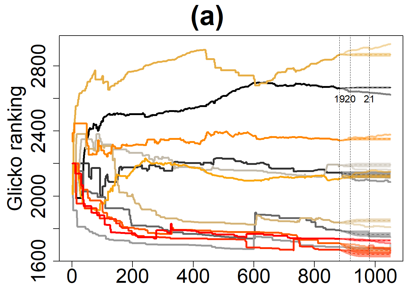
Figure 8: Further results on C-MMHP. (a) Glicko score ranking prediction of last three days using posterior draws, after fitting the first 18 days data in C-MMHP. True Glicko score ranking of all the time period is shown with the solid colored line, while the posterior prediction mean is in dashed line and one standard deviation is plotted in shaded color. The x-axis corresponds to the total number of interactions across the cohort. (b) Rank correlation between DSNL inferred latent rank and Glicko score ranking for each day in one cohort. Three colored bar indicated the performance of three inferred rankings conducted on the overall interactions, active and inactive respectively.

5 Discussion

In this paper, we propose a series statistical models that can uncover latent social dominance hierarchy among a group of animals from interaction win event times. These models can serve as an important tool in animal aggressive behavior analysis and provide insight into important questions of recognition and its role in hierarchy formation. To accomplish this, we formalize a point process model for continuous-time directed social network data. Three such models are developed: the cohort Hawkes process model (C-HP), the cohort degree-corrected Hawkes process model (C-DCHP) and the cohort Markov-modulated Hawkes process model (C-MMHP). The Hawkes process incorporates the winner effect and bursting patterns of aggressive behaviors, which are regularly observed in patterns of aggressive interactions across animal species. The degree correction allows the model to better capture individual level heterogeneity that is commonly observed in data of this form. Finally, Markov-modulation accounts for pair-flip situations and allows for asymmetry in interactions between pairs of animals, by separating these interactions into active and inactive states. Performing inference for these models in the Bayesian paradigm allows us to accurately quantify the uncertainty in the inferred rankings and to better infer the ranking of nodes involved in few interactions, components that have been lacking in existing models for animal ranking.

The simulation study demonstrates that inferences from these models are reasonable and that the true ranking of nodes can be recovered. The mice cohort study serves as a real data example and demonstrates that the C-MMHP model performs best overall, in terms of providing insightful latent rank inference, prediction of both events and rank over time and potentially being of interest in generating future research directions. Although we do not have a ground truth for rankings in real data, we have described how our model complements existing ranking methods in the literature and the potential value of the additional inference available. That the event dynamics can be described by a latent ranking provides evidence that how these mice interact and explore their social structure is driven by their position in a hierarchy, a key idea in recognition.

We explore the dynamics of animal behavior using this model motivated by observed and hypothesized phenomena in data of this form. The also highlight how the use of a new model may capture phenomena which existing models are not suited for. The results from our analysis of aggressive mice interactions provide insights on the agreement between model assumptions and the observed dynamics. This C-MMHP model can also be used to simulated future events, which could aid in designing studies of this form. Similarly, the state separation available in the C-MMHP model could lead to additional insights in conjunction with other models for animal behavior.

In the future, our model can be extended to incorporate the loser effect and bystander effect (Chase and Seitz,, 2011) within the Hawkes process intensity function. The loser effect means that an animal that has lost in earlier contests has an increased probability of losing subsequent contests with other individuals. The bystander effect describes the situation where an animal’s behavior might be influenced by observing an interaction or contest between two other animals. The extent of each effect can be estimated through a multivariate Hawkes process. The existence of such effects could be tested through the limiting distribution in Chen et al., (2017). Alternatively, models which utilise reciprocating interactions, such as Blundell et al., (2012) could also be of interest. So et al., (2015) raises a question about the causal relationship between aggressive behavior and gene expression. It is feasible to integrate these elements in our model by modeling the baseline intensities as a function of covariates that correspond to gene expression. We have also seen that certain global parameters in our models do not vary from Cohort to Cohort. As such, it would be of interest to design a hierarchical version of our model, borrowing strength from different datasets. Further work could also be done to make the degree estimates a function of the nodes latent rank, although there is no clear evidence from the literature as to the association between the baseline activity level and the position in a realised hierarchy. This question therefor remains an important future problem.

Similarly, the model we have proposed here is a special case of a latent space model. Latent space models are an important tool in social network analysis and have been widely used in modeling both static network (De Bacco et al.,, 2018; Hoff,, 2005; McCormick and Zheng,, 2015) and dynamic network (Sarkar and Moore,, 2006; Sewell and Chen,, 2015) data. Although latent space models of discrete-time dynamic networks have been considered (Kim et al.,, 2018), along with continuous time dynamics across repeatedly observed matrices (Durante and Dunson,, 2014), there has been little work in the context of continuous time events occurring on networks, and this remains an area for future research.

Data and Code

All data and code used in this paper are available in a public repository.

References

- Blundell et al., (2012) Blundell, C., Beck, J., and Heller, K. A. (2012). Modelling reciprocating relationships with hawkes processes. Advances in Neural Information Processing Systems, 25:2600–2608.
- Bonabeau et al., (1999) Bonabeau, E., Theraulaz, G., and Deneubourg, J.-L. (1999). Dominance orders in animal societies: the self-organization hypothesis revisited. Bulletin of mathematical biology, 61(4):727–757.
- Brown et al., (2002) Brown, E. N., Barbieri, R., Ventura, V., Kass, R. E., and Frank, L. M. (2002). The time-rescaling theorem and its application to neural spike train data analysis. Neural computation, 14(2):325–346.
- Carpenter et al., (2017) Carpenter, B., Gelman, A., Hoffman, M. D., Lee, D., Goodrich, B., Betancourt, M., Brubaker, M., Guo, J., Li, P., and Riddell, A. (2017). Stan: A probabilistic programming language. Journal of statistical software, 76(1).
- Chase and Seitz, (2011) Chase, I. D. and Seitz, K. (2011). Self-structuring properties of dominance hierarchies: a new perspective. In Advances in genetics, volume 75, pages 51–81. Elsevier.
- Chase et al., (2002) Chase, I. D., Tovey, C., Spangler-Martin, D., and Manfredonia, M. (2002). Individual differences versus social dynamics in the formation of animal dominance hierarchies. Proceedings of the National Academy of Sciences, 99(8):5744–5749.
- Chen et al., (2017) Chen, S., Shojaie, A., Shea-Brown, E., and Witten, D. (2017). The multivariate hawkes process in high dimensions: beyond mutual excitation. arXiv preprint arXiv:1707.04928.
- Daley and Jones, (2003) Daley, D. J. and Jones, D. V. (2003). An Introduction to the Theory of Point Processes: Elementary Theory of Point Processes. Springer.
- De Bacco et al., (2018) De Bacco, C., Larremore, D. B., and Moore, C. (2018). A physical model for efficient ranking in networks. Science advances, 4(7):eaar8260.
- de Vries, (1998) de Vries, H. (1998). Finding a dominance order most consistent with a linear hierarchy: a new procedure and review. Animal Behaviour, 55(4):827–843.
- de Vries and Appleby, (2000) de Vries, H. and Appleby, M. C. (2000). Finding an appropriate order for a hierarchy: a comparison of the i&si and the bbs methods. Animal Behaviour, 59(1):239–245.
- DeDeo and Hobson, (2021) DeDeo, S. and Hobson, E. A. (2021). From equality to hierarchy. Proceedings of the National Academy of Sciences, 118(21).
- Drews, (1993) Drews, C. (1993). The concept and definition of dominance in animal behaviour. Behaviour, 125(3):283–313.
- Dugatkin, (1997) Dugatkin, L. A. (1997). Winner and loser effects and the structure of dominance hierarchies. Behavioral Ecology, 8(6):583–587.
- Dugatkin and Earley, (2003) Dugatkin, L. A. and Earley, R. L. (2003). Group fusion: the impact of winner, loser, and bystander effects on hierarchy formation in large groups. Behavioral Ecology, 14(3):367–373.
- Durante and Dunson, (2014) Durante, D. and Dunson, D. B. (2014). Nonparametric bayes dynamic modelling of relational data. Biometrika, 101(4):883–898.
- Glickman, (1999) Glickman, M. E. (1999). Parameter estimation in large dynamic paired comparison experiments. Journal of the Royal Statistical Society: Series C (Applied Statistics), 48(3):377–394.
- Hawkes, (1971) Hawkes, A. G. (1971). Spectra of some self-exciting and mutually exciting point processes. Biometrika, pages 83–90.
- Hemelrijk, (2000) Hemelrijk, C. K. (2000). Towards the integration of social dominance and spatial structure. Animal behaviour, 59(5):1035–1048.
- Hobson, (2020) Hobson, E. A. (2020). Differences in social information are critical to understanding aggressive behavior in animal dominance hierarchies. Current opinion in psychology, 33:209–215.
- Hobson et al., (2021) Hobson, E. A., Mønster, D., and DeDeo, S. (2021). Aggression heuristics underlie animal dominance hierarchies and provide evidence of group-level social information. Proceedings of the National Academy of Sciences, 118(10).
- Hoff, (2005) Hoff, P. D. (2005). Bilinear mixed-effects models for dyadic data. Journal of the american Statistical association, 100(469):286–295.
- Hsu and Wolf, (1999) Hsu, Y. and Wolf, L. L. (1999). The winner and loser effect: integrating multiple experiences. Animal Behaviour, 57(4):903–910.
- Kim et al., (2018) Kim, B., Lee, K. H., Xue, L., Niu, X., et al. (2018). A review of dynamic network models with latent variables. Statistics Surveys, 12:105–135.
- Lee et al., (2019) Lee, W., Fu, J., Bouwman, N., Farago, P., and Curley, J. P. (2019). Temporal microstructure of dyadic social behavior during relationship formation in mice. PloS one, 14(12):e0220596.