Sensitivity and depth of investigation from Monte Carlo ensemble statistics

Abstract

For many geophysical measurements, such as direct current or electromagnetic induction methods, information fades away with depth. This has to be taken into account when interpreting models estimated from such measurements. For that reason, a measurement sensitivity analysis and determining the depth of investigation are standard steps during geophysical data processing. In deterministic gradient-based inversion, the most used sensitivity measure, the differential sensitivity, is readily available since these inversions require the computation of Jacobian matrices. In contrast, differential sensitivity may not be readily available in Monte Carlo inversion methods, since these methods do not necessarily include a linearization of the forward problem. Instead, a prior ensemble is used to simulate an ensemble of forward responses. Then, the prior ensemble is updated according to Bayesian inference. We propose to use the covariance between the prior ensemble and the forward response ensemble for constructing sensitivity measures. In Monte Carlo approaches, the estimation of this covariance does not require additional computations of the forward model. Normalizing this covariance by the variance of the prior ensemble, one obtains a simplified regression coefficient. We investigate differences between this simplified regression coefficient and differential sensitivity using simple forward models. For linear forward models, the simplified regression coefficient is equal to differential sensitivity, except for the influences of the sampling error and of the correlation structure of the prior distribution. In the non-linear case, the behaviour of the simplified regression coefficient as sensitivity measure is analysed for a simple non-linear forward model and a frequency-domain electromagnetic forward model. Differential sensitivity and the simplified regression coefficient are similar for prior intervals on which the forward model response is approximately linear. Differences between the two sensitivity measures increase with the degree of non-linearity in the prior range. Additionally, we investigate the correlation between prior ensemble and forward response ensemble as sensitivity measure. Correlation yields a normalised version of the simplified regression coefficient. We propose to use this correlation and the simplified regression coefficient for determining depth of investigation in Monte Carlo inversions.

1 Introduction

Many measurements used in applied geophysics, such as measurements from electrical resistivity tomography and electromagnetic induction methods, can be reproduced by assuming diffusive energy propagation. In combinations with simulations, such measurements allow to estimate subsurface distributions of physical properties, such as electrical conductivity, using inverse modeling techniques. There are two major types of inversion techniques, deterministic gradient-based and stochastic Monte Carlo (MC) inversions Aster et al., (2018). Both inversion types rely on the influence of proposed parametric subsurface models on simulation responses McGillivray and Oldenburg, (1990). The so-called measurement sensitivity characterises this influence by linearised analysis, i.e. partial derivatives of the simulated data with respect to model parameters. Using sensitivity, the influence of the different measurement signals can be compared. In particular, model parameters to which the measurements have negligible sensitivity can be identified.

For a typical surface measurement, sensitivity is negligible from a characteristic depth downwards. This characteristic depth is called the depth of investigation (DOI) of this particular surface measurement. An estimation of the DOI is crucial as it can prevent over- or misinterpretation of the inversion results Oldenburg and Li, (1999). A determination of the DOI is not trivial if data from diffusive methods are processed, since (1) a depth of absolute zero sensitivity does not exist, and (2) sensitivity computations are usually restricted to parameter variations around a (deterministic) inversion result. If the inversion result is significantly different from the true subsurface parameters, the estimation of the DOI may be wrong.

Due to the lack of a depth of truly zero sensitivity, a definition of the DOI always contains some degree of arbitrariness. Often, a rather small sensitivity threshold is defined relative to a reference sensitivity, for example using 5 $\%$ of the maximum sensitivity. Other approaches to DOI estimation define global sensitivity thresholds. For example, Christiansen and Auken, (2012) introduced the method of cumulative sensitivity. They compute all cumulative sums of sensitivities throughout a one-dimensional model starting from the bottom. This way, it is possible to give a global sensitivity threshold for DOI estimation, but the arbitrariness of this threshold remains. As the cumulative sensitivity is based on differential sensitivities, it must be assumed that the derived inverse image is a good representation of subsurface reality.

Despite the helpful guidelines for DOI estimation pointed out in the previous paragraph, the problem associated with investigating the sensitivity only around the final inverse model remains for deterministic inversion results. This non-uniqueness problem was already considered in the early days of geophysical inverse processing, for example using the Backus-Gilbert analysis (e.g., Backus and Gilbert, (1968) and Backus and Gilbert, (1967)). However, in their analysis, only a linear range around the result of the inverse method is searched for subsurface models that equally well satisfy the observed data. As a first step towards coping with this non-uniqueness problem in fully non-linear deterministic inversions, Oldenburg and Li, (1999) introduced the so-called DOI index for the interpretation of direct current and induced polarisation inversion results. This procedure was later adapted for the evaluation of electromagnetic inversion results (e.g., Brosten et al., (2011)). To derive the DOI index, the reference model for the inversion is altered to expose features in the inverse image that strongly depend on the choice of the reference model. However, alteration is often limited to two different reference models, leaving large parts of the model parameter space unexplored.

As an alternative to deterministic methods, stochastic Monte Carlo (MC) inversion methods have been used used more frequently in recent years as the available computational resources are growing Tarantola, (2005). Such methods solve the parameter estimation problem by random sampling of probability distributions and searching for an inverse solution given as a random parameter vector that follows a probability distribution as first formalized by Tarantola and Valette, (1982). MC methods tackle the general non-uniqueness problem by performing an as extensive as possible search of the model parameter space using random sampling. In this way, MC methods allow to characterise the uncertainty of the inversion result. Several variations of MC approaches exist and are used in geophysical practice. A thorough compilation, featuring popular applications of Markov chain Monte Carlo methods Mosegaard and Tarantola, (1995), can be found in Sambridge and Mosegaard, (2002). Although, since the publication of their review, several new MC methods have been introduced, for example trans-dimensional, multi-chain or approximate Bayesian methods (Malinverno, (2002), Sambridge et al., (2006), Socco and Boiero, (2008), Vrugt et al., (2009), and Bobe et al., (2019)).

In MC methods, the model parameter space that is sampled is defined based on prior knowledge. This prior knowledge can be understood in the Bayesian sense. It also serves as implicit regularization in such probabilistic frameworks. With its subjectivity, the definition of the prior is often the main criticism of Bayesian inversion methods Scales and Tenorio, (2001). However, in the following we will assume that defined prior distributions do reflect possible realizations of the subsurface according to prior knowledge.

Applying MC sampling, one has to compute the forward response for each prior model realization. Drawing a large number of prior samples, one obtains detailed insight on how changes in the parameter model relate to changes in the measurement response. Above, we defined such a relation as measurement sensitivity. Deriving covariance of the prior and the forward response ensemble and dividing this by the prior ensemble variance, we derive a simplified regression coefficient (SimRC). For dimensionless comparison of signals, the SimRC can be normalised by the variance of the forward response ensemble, yielding the correlation of prior and forward response ensemble.

Inversion updates derived from MC analysis are conditioned on the above mentioned covariances and the actual measurement data. Therefore, MC analysis does not require a linearised analysis of the forward problem and consequently, the traditionally used differential sensitivities are not readily available. Thus, commonly used DOI methods (see above) cannot immediately be applied. Moreover, local differential sensitivities have only limited informative value when evaluating results from global MC analysis and are usually not computed in such (e.g., Minsley, (2011)).

For DOI estimations in MC inversions, the inverted model is often cut at a depth at which posterior uncertainty becomes ’too large’ to be considered informative (e.g., Brodie and Sambridge, (2012)). One inconvenience of this DOI selection procedure is that the absolute size of the posterior uncertainty interval for model sections to which the measurements have negligible sensitivity almost only depends on the chosen prior probability. When a prior probability incorporates a high degree of certainty, a high degree of certainty will as well be seen for the posterior model, also for model parameters to which the measurements have vanishing sensitivity. This behaviour of the posterior probability makes a DOI threshold based on the size of the posterior uncertainty inevitably conditioned on the chosen prior distribution. Here, it should be noted that model sections with vanishing sensitivity or correlation to the measurements can certainly be considered just as reliable as the prior knowledge. Nevertheless, practitioners usually have keen interest in exploring the sensitivity of their model and in delineating their prior knowledge from the information gained from the inversion update.

One method for such a delineation is the computation of the Kullback-Leibler (KL) divergence. The KL divergence was recently presented for Bayesian inversion results in Blatter et al., (2018). The KL divergence gives the difference in information content of prior and posterior distribution. At a depth below prior and posterior distribution are near equal, no information was added by the measurement data. This depth can be interpreted as a DOI. However, the KL divergence is a purely statistical measure, allowing no analysis of measurement sensitivity and requires that a posterior distribution is available.

Analysis of the sensitivity not only gives insight in the nature of the inversion update, it can also support reconsideration of measurement design. However, instead of additionally computing differential sensitivities, we propose the use of the SimRC and of the correlation for model sensitivity analysis. The closely related regression coefficient as used by Saltelli et al., (2004) is often considered as a global sensitivity and is informative for the sampled model parameter space Saltelli et al., (2004). Additionally, the correlation allows for comparison of different measurement signals, and a vanishing correlation gives an intuitive measure for the DOI.

The text at hand treats the estimation of sensitivity and DOI for probabilistic MC inversion methods using the SimRC and correlation analysis. For some non-probabilistic MC methods (optimization methods), the presented work might be applicable, however, these will not be considered here. We will describe (1) how the readily available ensembles of prior distribution and forward response can be used to estimate SimRC sensitivity, and (2) how the SimRC and the corresponding correlation functions can be used to estimate a DOI. This DOI distinguishes between updated model parameters and parameters that essentially remain described by prior information. Additionally, common DOI estimation and illustration methods (e.g., Christiansen and Auken, (2012) and Oldenburg and Li, (1999)) can be applied to the SimRC functions.

The manuscript is structured as follows. First, we show how the SimRC is derived for Monte Carlo style inversions. Second, we explain how the SimRC relates to differential sensitivities in linear inverse problems. We also show how the SimRC and derived correlation functions can be used when estimating the DOI in surface measurement data inversions. Further, we include three synthetic studies illustrating differences and similarities between the differential sensitivity and the SimRC. We introduce a linear and a non-linear toy model to provide a semi-quantitative analysis of the influence of the prior distribution (sampling) specifications on the SimRC, namely prior correlation, non-linearity of the forward model, and the sample size. For the application to a geophysical problem, we provide simulations of a one-dimensional frequency-domain electromagnetic forward model in which different measurement signals with different differential sensitivities to the subsurface model are compared and analysed using the SimRC sensitivity.

2 Theory

In the following paragraphs we recall the general concept of Bayesian inference in Monte Carlo (MC) inversion approaches. Hereby, we will focus on the computation of the sample covariance between the prior and forward response ensemble. We motivate constructing measurement sensitivity measures from this covariance. The first proposed sensitivity measure is the covariance normalised by prior variance, a simplified regression coefficient (SimRC). We show that the SimRC and differential sensitivity are equal for the case of a linear forward model and no correlation in the prior distribution. Additionally, we propose using the SimRC and the correlation between prior ensemble and forward response ensemble for estimating the depth of investigation (DOI) of a geophysical surface measurement.

2.1 Bayesian inference

In Bayesian inversion approaches, prior information is represented in a probabilistic manner. According to Bayes’ theorem, this prior information is combined with the observed data to derive a posterior probability density function (PDF). The prior distribution is expressed as the PDF $\rho(\textbf{m})$ for the random vector of model parameters $\textbf{m}\in\mathbb{R}^{n_{par}}$, where $n_{par}$ is the number of model parameters. The likelihood function is the PDF $\rho(\textbf{d}|\textbf{m})$ that denotes the conditional probability that a set of observation $\mathbf{d}\in\mathbb{R}^{n_{obs}}$ is measured for a given set of parameters. Here, $n_{obs}$ denotes the number of observation variables. For geophysical measurements, the likelihood gives information on whether an observation is compatible with predicted responses $g(\textbf{m})$, where $g$ is a geophysical forward model. The posterior PDF for the random vector of model parameters is derived by applying Bayes’ theorem:

$$\rho(\textbf{m}|\textbf{d})\propto\rho(\textbf{d}|\textbf{m})\rho(\textbf{m}).$$ (1)

For large-dimensional non-linear inverse problems, no analytical solution to Equation 1 can be given Tarantola, (2005). Numerical sampling of the involved probability distributions is one possibility for obtaining an approximate solution to Bayes’ theorem. Monte Carlo methods are a class of algorithms based on numerical random sampling. Collecting the Monte Carlo samples in matrices, we approximate $\rho(\textbf{m})$ by a matrix $\mathbf{M}\in\mathbb{R}^{(n_{par}\times N)}$ Evensen, (2003), where $N$ is the number of samples. For each column in $\mathbf{M}$, forward responses are simulated. The resulting forward response ensemble is collected in a matrix $\mathbf{G}=g(\mathbf{M})\in\mathbb{R}^{(n_{obs}\times N)}$.

In principle, drawing a large number of samples $N$ the model parameter space is searched nearly exhaustively covering almost all possible parameter realizations. In comparison with deterministic inversion, non-uniqueness problems are therefore largely mitigated in MC inversions Tarantola and Valette, (1982).

We start the introduction of the SimRC by defining the covariance matrices between the parameters $\mathbf{m}$ following the prior distribution $\rho$, and the forward model responses $g(\mathbf{m})$:

$$\mathrm{Cov}(g(\mathbf{m}),\mathbf{m})=\mathbf{E}[(\mathbf{m}-\mathbf{E}[\mathbf{m}])(g(\mathbf{m})-\mathbf{E}[g(\mathbf{m})])^{T}].$$ (2)

The covariances $\mathrm{Cov}(\mathbf{m},\mathbf{m})$ and $\mathrm{Cov}(g(\mathbf{m}),g(\mathbf{m}))$ are defined analogously. In Figure 1, we summarise the sensitivity measure candidates of this work that are derived from these covariances.

From now on, we express probability distributions by an ensemble of Monte Carlo samples. Consequently, the covariances will be approximated as sample covariances. In terms of the ensemble matrices $\mathbf{M}$ and $\mathbf{G}$ the approximation of the covariance $\mathrm{Cov}(g(\mathbf{m}),\mathbf{m})$ reads

$$\mathbf{C}_{mg}:=\mathbf{M^{\prime}G^{\prime}}^{T}\frac{1}{N-1}\approx\mathrm{Cov}(g(\mathbf{m}),\mathbf{m}),$$ (3)

where the primed matrices denote that for each parameter the parameter mean was subtracted from each parameter sample. Analogously, we define the (co-)variance matrices

$$\mathbf{V}_{m}:=\mathbf{M^{\prime}M^{\prime}}^{T}\frac{1}{N-1}\approx\mathrm{Cov}(\mathbf{m},\mathbf{m}),$$ (4)

and

$$\mathbf{V}_{g}:=\mathbf{G^{\prime}G^{\prime}}^{T}\frac{1}{N-1}\approx\mathrm{Cov}(g(\mathbf{m}),g(\mathbf{m})).$$ (5)

In this notation, the sample approximations for the various coefficients given in Figure 1 can be summarized as follows:

$$\mathrm{RC}_{j,i}=[\mathbf{V}^{-1}_{m}\mathbf{C}_{mg}]_{i,j}\qquad\mathrm{(regression\,\,coefficient)},$$ (6)

and

$$\mathrm{SRC}_{j,i}=[\mathbf{V}^{-1}_{m}\mathbf{C}_{mg}]_{i,j}(\sigma_{m_{i}}/\sigma_{g_{j}})\qquad\mathrm{(standardized\,\,RC)}$$ (7)

by Saltelli et al., (2004), where the index $j$ is used for responses and the index $i$ is used for model parameters. Consequently, the pair $ji$ could be read as sensitivity of response $j$ on parameter $i$.

Additionally, we define

$$\mathrm{SimRC}_{j,i}=[\mathbf{C}_{mg}]_{i,j}/\sigma^{2}_{m_{i}}\qquad\mathrm{(simplified\,\,RC)},$$ (8)

and

$$\mathrm{CC}_{j,i}=[\mathbf{C}_{mg}]_{i,j}/(\sigma_{m_{i}}\sigma_{g_{j}})\qquad\mathrm{(correlation\,\,coefficient)},$$ (9)

where $\sigma^{2}_{m_{i}}:=[\mathbf{V}_{m}]_{ii}$ and $\sigma^{2}_{g_{j}}:=[\mathbf{V}_{g}]_{jj}$ are the sample variances.

The comparison of various correlations, for example CC, can be easier than the comparison of covariances, as correlation is independent of units by normalization Mosegaard and Tarantola, (1995).

2.2 Discussion of the SimRC

SimRC vs. differential sensitivity

Sensitivities characterise the influence of a parameter model on simulated measurement responses. Sensitivities are used for communicating geophysical inversion results as they support interpretation and possibly hint at adjustments of measurement design. Mostly, sensitivities are derived from a differential analysis, i.e. applying the difference quotient. For MC analysis, where Jacobian approximations are not readily available, we propose the usage of the SimRC as defined in the previous section. To illustrate similarities between SimRC and differential sensitivity, we now consider a linear forward model.

Linear forward models

We give the linear forward model of finite dimensions $g:\mathbb{R}^{n_{par}}\rightarrow\mathbb{R}^{n_{obs}}$ the following general form:

$$g(\mathbf{m})=\mathbf{A}\cdot\mathbf{m}+\mathbf{b},$$ (10)

with vector $\mathbf{b}$ for the intercept and matrix $\mathbf{A}\in\mathbb{R}^{(n_{obs}\times n_{par})}$ for the slope. Arbitrary samples of $\mathbf{m}$ can be used to generate a $(\mathbf{m},g(\mathbf{m}))$-scatter plot, in which all points lie on the plane defined by Equation 10.

Using the property of the sample covariance matrix that it is a quadratic form (Horn and Johnson, (2012); chapter 4.5.3), we get

$$\mathrm{Cov}(\mathbf{m},g(\mathbf{m}))=\mathrm{Cov}(\mathbf{m},\mathbf{m})\mathbf{A}^{T}.$$ (11)

Here, $\mathrm{Cov}(\mathbf{m},\mathbf{m})\in\mathbb{R}^{(n_{par}\times n_{par})}$ is the prior covariance matrix of the parameter vector. Inserting the Monte Carlo samples, we get the expression

$$\mathbf{C}_{mg}=\mathbf{V}_{m}\mathbf{A}^{T}.$$ (12)

We now use (1) that quadratic covariance matrices are invertible (in the definition of RC), and (2) the general identity $\mathrm{Cov}(\mathbf{x},\mathbf{y})^{T}=\mathrm{Cov}(\mathbf{y},\mathbf{x})$.

Inserting Equation 12 in the definition of RC and SRC (Eq. 6 and 7), one derives

$$\mathrm{RC}_{j,i}=[\mathbf{A}]_{j,i}.$$ (13)

In this linear case, this slope $\mathbf{A}$ is equal to both the differential sensitivity and the regression coefficient as used by Saltelli et al., (2004).

If the prior covariance matrix is a simple diagonal matrix, or equivalently no prior correlation is implemented, the relation $[\mathbf{C}_{mg}]_{i,j}=\sigma^{2}_{m_{i}}[\mathbf{A}]_{j,i}$ holds, and then can be inserted in the SimRC definition (Eq. 8), yielding the same expression as for RC_j,i in Equation 13.

Non-diagonality

For non-diagonal prior covariance matrices, the SimRC differs from the general regression coefficient/differential sensitivity due to the simplified matrix inversion.

In this work, we propose the SimRC for construction of sensitivity measures for two reasons. First, prior correlation has a strong effect on Bayesian inference and thus, it may be beneficial to incorporate it in a sensitivity measure. Monte Carlo samples of the prior distribution account for prior correlation. Likewise, the SimRC functions implicitly include prior correlation. Second, the computation of the SimRC is less expensive compared to the computation of the regression coefficient as given in Equation 6. For some cases, specifically for large models, the sample model variance matrix $\mathbf{V}_{m}=\mathbf{M^{\prime}M^{\prime}}^{T}/(N-1)$ (see Eq. 4) may be singular. This singularity causes the non-existence of the matrix’ inverse, disallowing the computation of RC and SRC.

Non-linearity

For non-linear functions $g$, the slope at point $\mathbf{m}$ is computed using the difference quotient:

$$\frac{\partial g_{j}(\mathbf{m})}{\partial m_{i}}\approx\frac{g_{j}(\mathbf{m}+\Delta m\mathbf{e}_{i})-g_{j}(\mathbf{m})}{\Delta m},$$ (14)

for which the $i$th parameter was perturbed by $\Delta m$, and $\mathbf{e}_{i}$ is its unit vector. From the linear case, we can draw some conclusions regarding the relation of difference quotient and SimRC for general functions. The difference quotient and the SimRC should be approximately equal for prior parameters ranges that are in the order of $\Delta m_{i}$. Below, we will investigate the similarity of the SimRC and the difference quotient for two synthetic non-linear forward models. In practice the search space defined through the prior distribution is large compared to an infinitesimally small $\Delta m_{i}$. Thus, in the context of general non-linear forward models, the SimRC needs to be interpreted by comparing the prior parameter range to the non-linearity of the forward model.

2.3 Correlation and depth of investigation

Often, an estimate for the depth of investigation (DOI) and sensitivity functions are provided along with inversion results. In probabilistic inversions, inversion results should be as least as reliable as the prior knowledge, regardless of how sensitive or insensitive the surface measurements are to the parameters. However, also for probabilistic inversions, sensitivity and DOI allow valuable insight into the nature of the inversion process. In particular, they can help to distinguish between parameters updated by Bayesian inference and parameters left more or less at their prior values. In this way, sensitivities and DOI may point out that an adjustment of measurement design is necessary.

The SimRC gives a measure for the sensitivity of a measurement setup to a particular subsurface model. Thus, all available approaches for determining the DOI from sensitivity can be applied to the SimRC. However, for determining the DOI, a dimensionless sensitivity can have advantages. By normalizing the SimRC, one obtains the correlation between prior ensembles and forward response ensembles (Eq. 9). This correlation can be viewed as standardised SimRC corresponding to the standardised regression coefficient as used by Saltelli et al., (2004).

Due to its normalization, the correlation function has some beneficial properties when compared to the SimRC. First, the normalization makes sensitivities of different measurement signals comparable and easier to threshold. For example, the influence of signals from different electrode configurations in a direct current resistivity survey can be compared in terms of correlation. Second, for parameters with zero correlation to the measurement setup, no inversion update will be seen. Thus, zero correlation gives an intuitive measure for the DOI of Bayesian inference: the depth below which almost no correlation is found. One disadvantage of using correlation as sensitivity measure is that strong correlation can happen while there is small sensitivity (for a wide range of applicable parameter values). Thus, the information of how wide the range of equally applicable parameter values is, is lost by normalization.

To complete the discussion of using the correlation for determining the DOI, we discuss the selection process. Due to two reasons a zero correlation DOI cannot be determined: (1) as for other sensitivity measures, the diffusive nature of energy propagation for the discussed measurement techniques prevents the correlation from reaching the zero function, and (2) the presence of undersampling in the MC ensemble may introduce spurious correlation.

Due to reason (1) there is always some degree of arbitrariness in the DOI threshold selection. Thanks to its normalization and the resulting comparability between parameters, the correlation allows the definition of global DOI threshold values (for global DOI threshold values derived from differential sensitivity see Oldenburg and Li, (1999) and Christiansen and Auken, (2012)).

Regarding reason (2), as always in ensemble calculations, the ensemble has to be chosen large enough such that the spurious correlations are kept in the background noise.

A useful approach accounting for fluctuations when determining the DOI from correlation sensitivity is the upwards cumulative sensitivity approach by Christiansen and Auken, (2012). This approach can easily be applied to the CC functions (Eq. 9). By computing a cumulative sum, the possibly present spurious correlation is smoothed. To enable global thresholding, we introduce a normalization:

$$\mathrm{CC}^{cum}_{j}(\mathbf{M,G})=\frac{\sum\limits_{i=j}^{n_{par}}|\mathrm{CC}_{i}|}{|\mathrm{CC}_{max}|},$$ (15)

with indices $j=1,...,n_{par}$, the correlation sensitivity $\mathrm{CC}_{i}$ for the $i$th layer, and the maximum correlation sensitivity $\mathrm{CC}_{max}$ for the vertical sequence of parameters.

The upwards cumulative sensitivity approach will be analysed in the synthetic examples below.

3 Synthetic examples

We now investigate the differences between differential sensitivity on the one hand, and the simplified regression coefficient (SimRC, Equation 8) and the correlation coefficient (CC, Equation 9) on the other hand. To this end, we look at the depth distribution of these parameters and use them to estimate a depth of investigation (DOI) for interesting cases. As outlined above, we expect that the differences between differential sensitivity and the SimRC are essentially determined by three parameters: (1) non-linearity of the physical model equations, (2) prior distribution correlations, and (3) the sampling bias of the ensemble. First, a linear toy model is used to illustrate the influence of sampling bias and prior correlation for the linear case. Second, for a non-linear toy model all three influencing parameters are investigated. Finally, we analyse the SimRC and correlation for a non-linear geophysical model and compare them to differential sensitivities.

3.1 Linear toy model

We start with the relation of differential sensitivity and the SimRC using the simple case of a linear toy model. This toy model describes a surface measurement $S$ that is sensitive to a subsurface property $p$. The toy model is characterised by two key features: (1) a linear relation between the model parameters and the model response, and (2) an exponential decrease of the model response with depth. This exponential behaviour introduces a sensitivity that converges to zero with increasing depth but, similarly to diffusive geophysical models, a depth of truly zero sensitivity does not exist.

We choose the explicit relation between measurement response $S$ and subsurface parameter $p$ as follows

$$S(z)=S_{0}\cdot\frac{p}{p_{0}}\cdot\mathrm{e}^{-z/z_{0}},$$ (16)

with depth $z$, and constants $S_{0}$, $p_{0}$ and $z_{0}$. $S_{0}$ is the response of a subsurface layer with property $p_{0}$ at negligible depth. $z_{0}$ is the depth at which the response of a subsurface layer is reduced by a factor $1/\mathrm{e}$ compared to negligible depth. In general, these constants depend on the units of the corresponding physical variable. For simplicity, we set them to one.

The total toy model response is given by an integration over the whole subsurface:

$$S^{total}=\int_{0}^{\infty}S(z)\mathrm{d}z.$$ (17)

We discretise Equation 17 using equally thick, discrete layers of constant $p$. The bottom layer of the model is chosen to extend to infinite depth. In the following, we investigate the two influences on the relation of the SimRC and differential sensitivity expected from theory: (1) different prior distribution probability density functions (PDFs), and (2) the influence of the ensemble size on the RC.

We define some standard parameters that remain valid for all comparisons unless explicitly stated otherwise. First, each prior distribution is sampled drawing 100,000 samples. The standard deviations (STDs) of the respective forward responses are computed from the ensemble. We define a prior distribution with identical Gaussian prior PDFs for each discrete model layer: a mean of $p=3$ and a STD of 0.5. We compute the SimRC and correlation between the prior ensemble and the forward response ensemble computed by the linear toy model. We compare the SimRC function to the differential sensitivity for a homogeneous parameter model at $p=3$.

3.1.1 Gaussian prior PDF

We study the SimRC and the correlation for the linear toy model using five different prior STDs: 0.01, 0.1, 0.5 , 1.0, and 1.5.

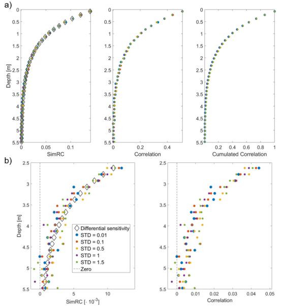
Figure 2: a) Differential sensitivity, simplified regression coefficient (SimRC; left) and correlation (center, right) for five prior standard deviations (STD). Forward responses are computed using the linear toy model; b) Zoom-in of a).

Results for the SimRC, correlation, and differential sensitivity are shown in Figure 2a. As described by the toy model (Eq. 16), the differential sensitivity asymptotically approaches the zero function with depth. As expected for linear model equations, all SimRC functions (Eq. 8) are very close to the differential sensitivity function. The shape of all correlation functions (Fig. 2a center) is similar to the differential sensitivity function. As a consequence, the cumulative correlation functions are very similar for all five prior distribution STDs.

We now zoom in the results (Fig. 2b) in order to visualise sampling fluctuations. On average, the SimRC follows the differential sensitivity function. However, fluctuations around the differential sensitivity are present for all derived SimRC functions. Such fluctuations can be explained by the sampling bias.

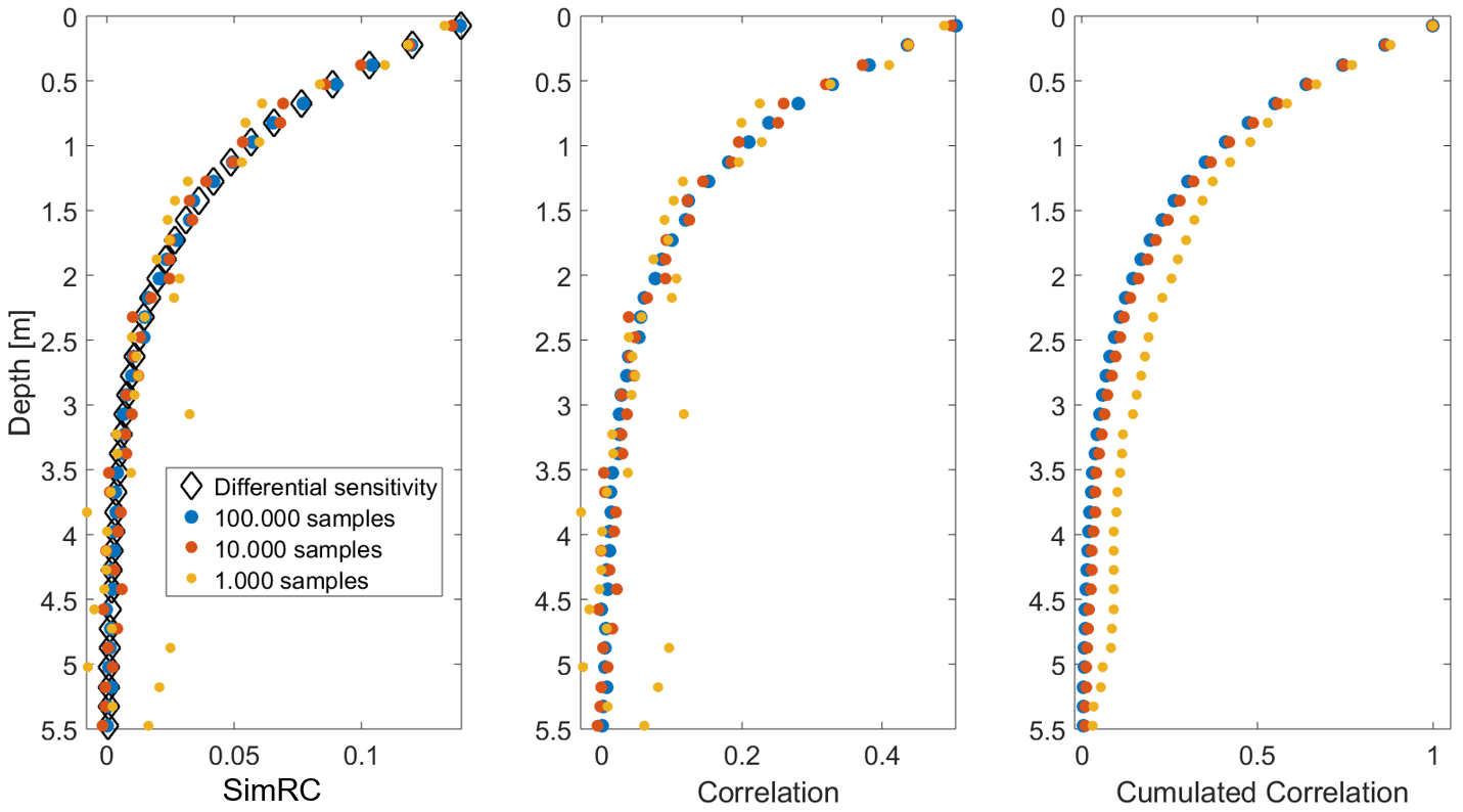
Figure 3: Differential sensitivity, simplified regression coefficient (SimRC; left) and correlation (center, right) for three different ensemble sizes. Forward responses are computed using the linear toy model.

To investigate the influence of the ensemble size on the SimRC and correlation functions, we re-sample the Gaussian prior PDF with a STD of 0.5 using the smaller ensemble sizes 10,000 and 1,000. Results are shown in Figure 3. The comparison with differential sensitivity indicates the expected increase in the sampling error with decreasing ensemble size. The sampling error is also present in the different cumulative correlation functions. By normalizing and summing up, the fluctuations are smoothed and they stay visible as an offset generated by the larger absolute correlation values at depth.

For an ensemble of only 1,000 samples, the undersampling effects become so pronounced that they prevent the interpretation of the SimRC as sensitivity. Thus, for this toy model, an ensemble size of at least 10,000 is needed to use the SimRC as sensitivity, and subsequently for defining a DOI. However, it is important to note here that the minimal necessary number of samples in other studies may differ and always depend on the specific problem addressed.

Theoretically, differential sensitivities can only take positive values for this toy model. Thus, negative sensitivity values are a result of sampling error. Generally, negative sensitivity values should only occur in regions below the DOI. For such profile sections to which measurements have low sensitivity, the correlation must be interpreted as zero, or, in the case of interpreting results from diffusive methods, as negligibly small.

The DOI derived from the differential sensitivity using a threshold of 5 $\%$ of the maximum sensitivity is 3 meter. Since the SimRC values are almost equal to the differential sensitivities, they yield a DOI of 3 meter as well. For the correlations and cumulative correlation, we choose the thresholds that yield the same DOI of 3 meter in this simple linear case. For the correlations, this threshold correlation is 0.03. For cumulative correlation, this threshold is 0.05. For the more complicated examples, we will analyse the differences in DOI for these same thresholds.

3.1.2 Multivariate Gaussian prior PDF with vertical constraints

To study the effect of prior correlation on the SimRC, we investigate four prior distributions with different correlation lengths. In general, prior correlation is implemented if a priori correlation between model parameters is assumed Tarantola and Valette, (1982). We extend the separate Gaussian PDFs per parameter to a multivariate Gaussian PDF (e.g., Mardia et al., (1979)). In this multivariate Gaussian PDF, parameters can be correlated via a prior covariance matrix Hansen et al., (2006). Here, we introduce a simple Gaussian shaped correlation, which is fully defined by a standard deviation of the prior parameters and a spatial correlation length (Gaspari and Cohn, (1999); Section 4.3). As before, for all parameters the Gaussian mean is set to $p=3$ and a STD of 0.5 is chosen, creating a multivariate Gaussian prior distribution. We compute multiple ensembles for different prior distributions with increasing correlation length: 0 m, 0.2 m, 0.6 m and 1m. For the correlation length of zero meters, parameters are sampled independently, and thus, this prior distribution is equivalent to the uncorrelated Gaussian PDFs of the last section.

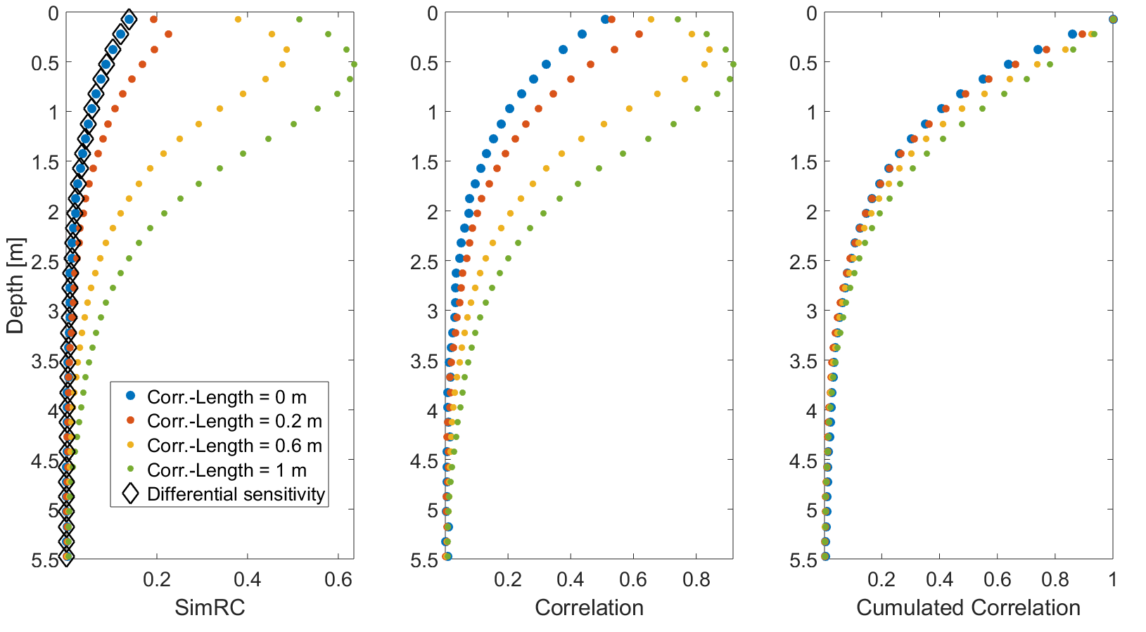
Figure 4: Differential sensitivity, simplified regression coefficient (SimRC; left) and correlation (center, right) for four different correlation lengths of a uniform multivariate Gaussian prior distribution. Forward responses are computed using the linear toy model.

SimRC results for different correlation lengths are shown in Figure 4. The larger the prior correlation length, the larger the SimRC and consequently the correlation between prior ensemble and forward response ensemble. Prior correlation has the most obvious effect on the shallow parameters to which measurements are more sensitive. For the very shallowest parameters, correlation decreases again due to the decreasing number of neighbouring correlated layers.

The difference between differential sensitivity and the SimRC caused by prior correlation has to be taken into account when interpreting SimRC functions as sensitivity. On the one hand, this is a deviation from the concept of differential sensitivity derived purely from partial derivatives. On the other hand, it may be beneficial, especially in Bayesian inversion methods, to incorporate the prior correlation into the sensitivity measure since it drives the Bayesian update. Of course, when interpreting the SimRC, it has to be kept in mind that the SimRC is not purely a property of the functional relationship at hand. Instead, it is influenced by a mixture of the functional relationship and the prior correlation that is a human input. Finally, for the cumulative correlation functions, we can observe that the differences due to correlation are reduced by the normalization (Fig 4 right).

Since an increase in correlation length leads to larger SimRC values, it is evident that it also enlarges a DOI estimate that is derived from SimRC and correlation analysis. As before, we use 5 $\%$ of the maximum sensitivity as the DOI threshold to compare DOIs estimated from differential sensitivity and SimRC functions. For the DOIs derived from correlation, we use a threshold correlation of 0.03. For the cumulative correlation we choose 0.05 as DOI threshold. These two threshold are set based on the results of the previous examples (see above).

All DOI values are listed in Table 1. The DOI for differential sensitivity is 3 meter. For the SimRC and the correlation, the derived DOIs are larger for larger correlation lengths. This behaviour has the same advantages and disadvantages as the form of the SimRC function as discussed before. The disadvantage is that the DOI is affected by input other than the function itself. On the other hand, the advantage is that the larger DOI properly reflects the sphere of influence of the Bayesian update. For the cumulative correlation, the DOIs are closer to the DOI of the differential sensitivity. We attribute this to the normalization that also brings the cumulative correlation curves closer together.

3.2 Non-linear toy model

To study differences between differential sensitivity and the SimRC for a non-linear parameter dependence, we introduce a simple but strongly non-linear toy model. We adjust the linear toy model from the previous section by turning the linear relation between the model response and the subsurface parameter $p$ into an exponential one (Figure 5):

$$S(z)=S_{0}\cdot\mathrm{e}^{p/p_{0}}\cdot\mathrm{e}^{-z/z_{0}}.$$ (18)

The total response is computed for a discretised model analogous to the linear case. As for the linear example, we compute SimRC and correlation of prior and forward response ensemble for different prior distributions and ensemble sizes. As before, the default prior distribution is a Gaussian PDF with mean $p=3$ and STD of 0.5, sampled using an ensemble size of 100,000, unless stated otherwise.

3.2.1 Gaussian prior PDF

We study the effect of the non-linearity between the forward model response and the prior distribution by using five prior distributions differing in STD. The STDs are 0.01, 0.1, 0.5 , 1.0, and 1.5. For larger STD, the ensemble will be more non-linear.

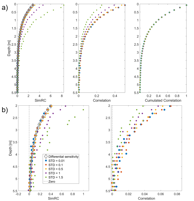
Figure 6: a) Differential sensitivity, simplified regression coefficient (SimRC; left) and correlation (center, right) for five prior standard deviations (STD). Forward responses are computed using the non-linear toy model; b) Zoom-in of a).

Results are shown in Figure 6. For the two smallest STDs, the SimRC function (Eq. 8) is close to the differential sensitivities (Fig. 6a left). In the more shallow profile sections, we observe that the SimRC increases for the larger STDs. As the parameter-response relation is exponential, this behaviour is expected. For the larger STDs, the curvature of the non-linearity of the forward model leads to regression coefficients that are larger than the slope at the mean of the prior ensemble. If the curvature had a different sign, such that it would reduce the slope of the function, it would lead to SimRC values that are smaller than differential sensitivity.

In the correlation functions (Fig. 6), we see that an increase in prior STD causes a decrease in the correlation for the more shallow model parameters. As correlation is a measure for the linearity of the relation between two random variables, this decrease of correlation is expected for the non-linear toy model. For correlation, any curvature would lead to a decrease. The cumulative correlation function is similar for all investigated prior STDs (Fig. 6a right). The integration over depth almost removes the effects of the non-linearities in the correlation functions. Thus, a DOI estimation derived from cumulative correlation functions would be almost identical for all STDs.

For the SimRC, fluctuations around the differential sensitivity function are observed especially in the lower most parts of the profile (Fig. 6b). Fluctuations are more pronounced for larger STDs. Thus, a strong non-linearity in parameter-response relation requires a larger ensemble size to achieve a similarly low degree of ensemble bias as seen for less non-linear relations.

Turning to the DOIs, we use the same threshold as for the linear case. For the differential sensitivity, this results in a DOI of 3 m. All DOI values are listed in Table 2. SimRC DOIs are close to the 3 meter DOI derived for the differential sensitivity function, regardless of the prior distribution STD. For the DOI derived from the correlation functions, a decrease in DOI is observed for an increasing prior STD. This effect can be traced back to the general decrease of correlation for an increasing non-linearity (see above). As for the linear example, the cumulative correlation is closer to the DOI derived for differential sensitivity by normalization.

3.2.2 Multivariate Gaussian prior PDF with vertical constraints

As for the linear case, we now introduce prior correlation by turning the Gaussian priors from the previous section into multivariate Gaussian priors. The SimRC is analysed for these correlation lengths: 0 m, 0.2 m, 0.6 m and 1m.

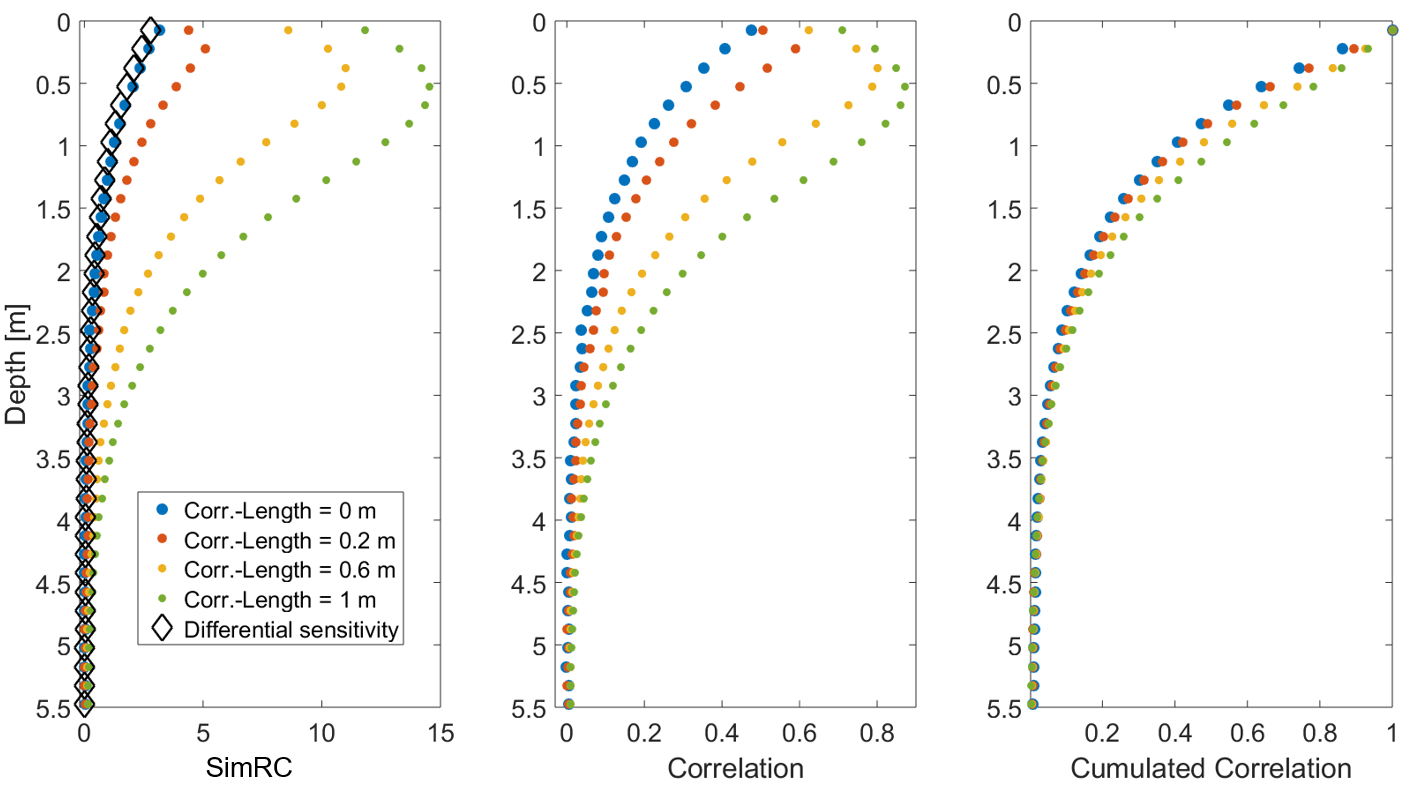
Figure 7: Differential sensitivity, simplified regression coefficient (SimRC; left) and correlation (center, right) for four different correlation lengths of a uniform multivariate Gaussian prior distribution. Forward responses are computed using the non-linear toy model.

Results are shown in Figure 7. By comparing the SimRC to differential sensitivity, we see two influences on the SimRC functions: (1) a relatively small offset arising from the non-linearity in the model response, and (2) the relatively larger influence of the prior correlation. As for the linear case, the SimRC and correlation in the shallow profile parts increase with increasing correlation length as parameters here are most sensitive to the toy model.

Since the sensitivity measures for this case are very similar case with correlation, we do not explicitly show the DOI values. As in the linear case, the DOI estimates for the SimRC in the region of enhanced correlation are larger compared to the DOI estimate from differential sensitivity.

3.2.3 Uniform prior PDF

We study the applicability of SimRC and correlation analysis of uniform PDFs as a simple non-Gaussian case. We study the non-linearity of the toy model response by increasing the size of the prior interval. In particular, we derive the SimRC and correlation functions for five different uniform prior intervals around a mean of $p=3$: $\pm$0.05, $\pm$0.5, $\pm$2.5,$\pm$5.0, and $\pm$7.5.

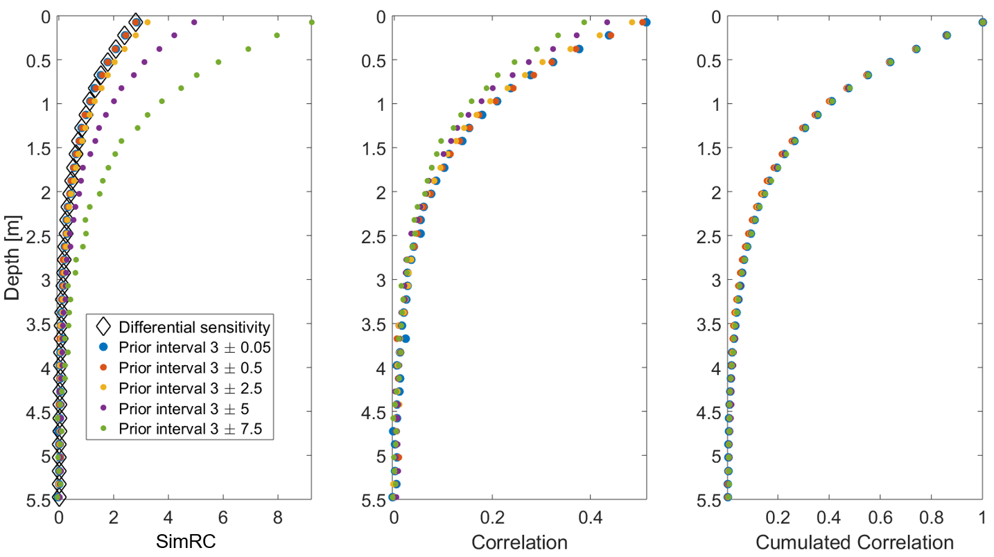
Figure 8: Differential sensitivity, simplified regression coefficient (SimRC; left) and correlation (center, right) for five uniform prior intervals. Forward responses are computed using the non-linear toy model.

Results are shown in Figure 8. The SimRC and correlation functions are similar to the Gaussian case. Again, for the two smallest prior intervals, the differential sensitivity approximately equals the computed SimRC. As for the Gaussian case, correlation decreases with an increase of non-linearity on the investigated parameter-response interval. The cumulative correlation functions are closer together for all investigated prior distribution PDFs. This simple example shows that the usage of SimRC and correlation as sensitivity measures is not strictly restricted to Gaussian PDFs.

3.3 Frequency-domain electromagnetic model

Frequency-domain electromagnetic (FDEM) induction data show diffusive energy propagation in the subsurface when low frequencies are used for surveying. Therefore, measurement sensitivity and DOI are quantities of interest when FDEM are processed and discussed.

FDEM data are sensitive to the electrical conductivity (EC) of the subsurface. During FDEM surveys, an electromagnetic field is generated in a transmitter coil. The field propagates into the subsurface and generates eddy currents in conductive material. These eddy currents subsequently generate a secondary field that is recorded by one or multiple receiver coils. The magnitude of the secondary field is usually expressed in parts-per-million [ppm] with respect to the primary field. This magnitude can be related to EC using the non-linear formulas given by Ward and Hohmann, (1988).

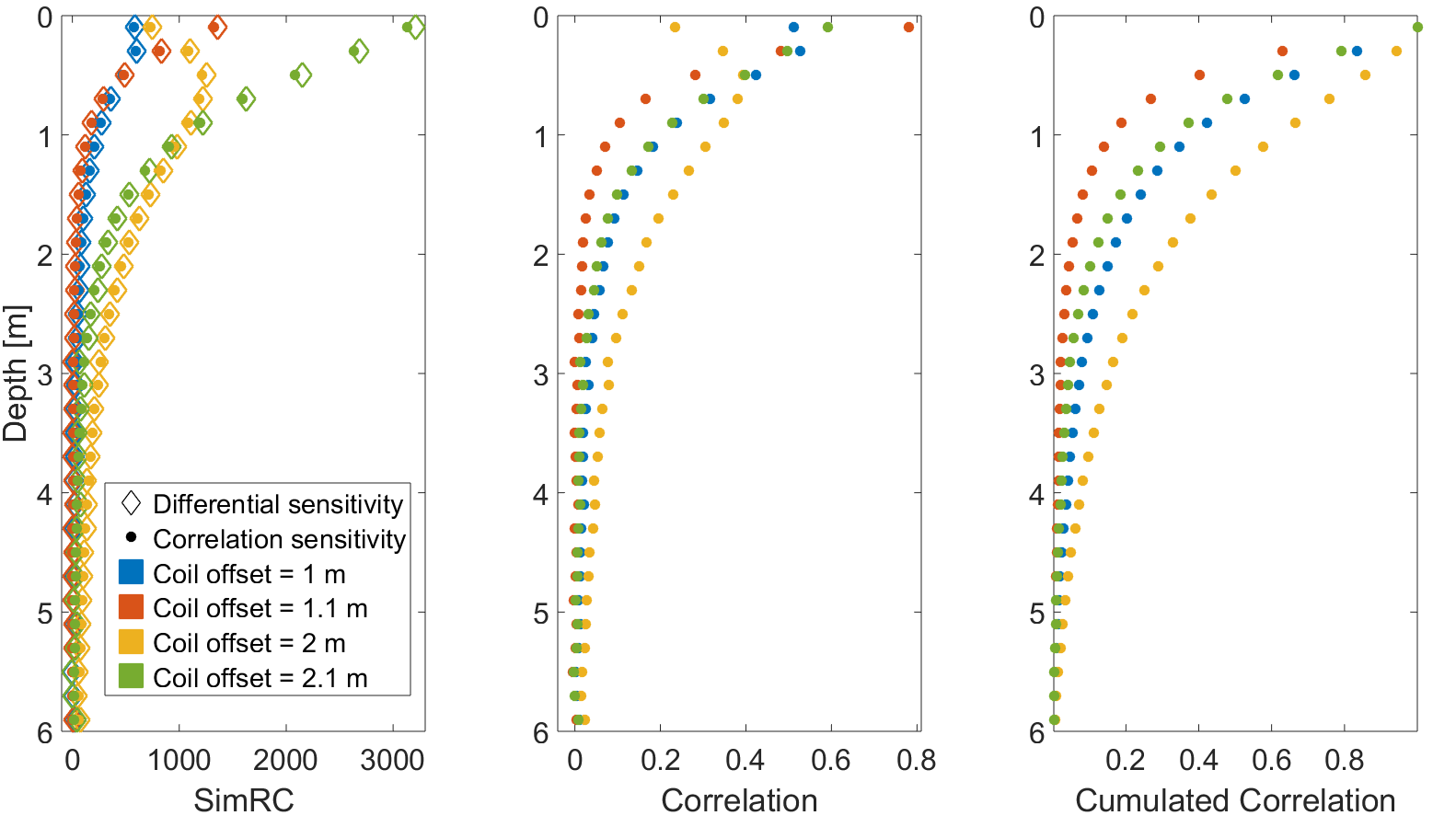
Figure 10: Differential sensitivity, simplified regression coefficient (SimRC; left) and correlation (center, right) for a uniform Gaussian prior distribution and the different simulated measurement signals for four FDEM receiver coils with different distance to the transmitter coil.

For one-dimensional forward modelling of FDEM data, we use the code provided by Hanssens et al., (2019). We simulate data for one transmitter and two receiver coils, each of the receivers simulated at two different lateral offsets. The first receiver is simulated with a horizontal co-planar coil setup at two locations, in particular at 1 m and 2 m offset to the transmitter coil. The second receiver is simulated with a perpendicular coil setup at 1.1 m and 2.1 m offset from the transmitter coil. This way, simulated differential sensitivity functions (Fig. 10) of the four signals differ (1) in magnitude due to the offset variations, and (2) in shape due to the difference in setup geometry.

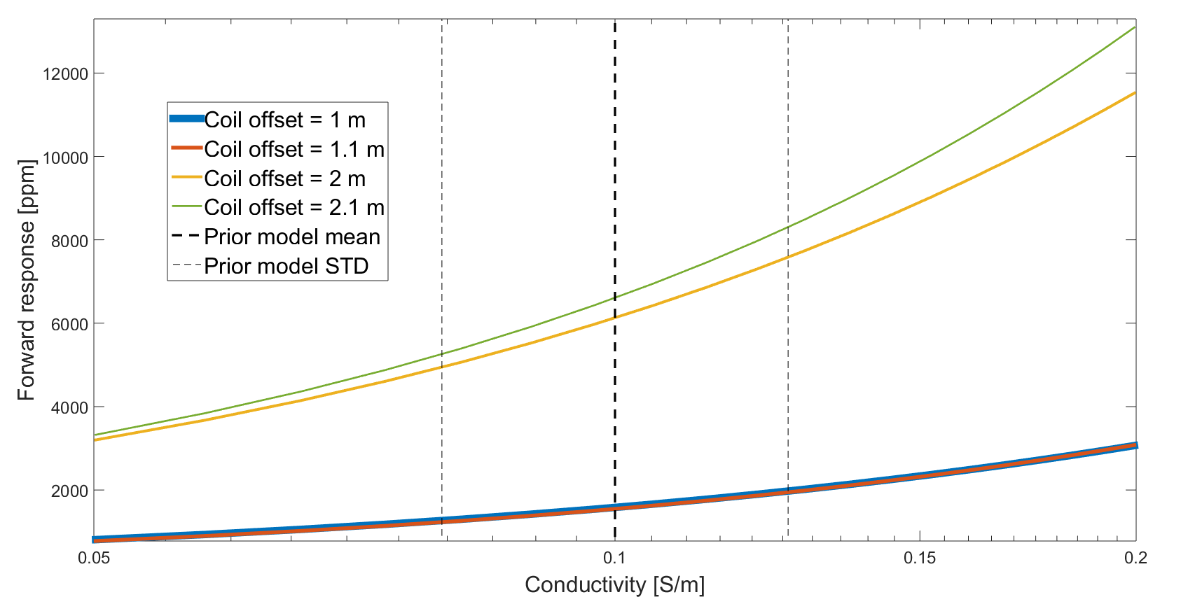
Figure 9: Forward response for the FDEM forward model around the Gaussian prior distribution mean.

Data are simulated for a discretised subsurface for which each layer is 20 cm thick. To prevent unphysical (negative) parameter values, prior model parameters are defined through log-normal PDFs for the subsurface parameters. The prior ensemble has a size of 100,000. Around the selected prior mean (EC of 100 mS/m), the forward response shows a slightly non-linear behaviour (Fig. 9). For the coils with larger offset, the non-linearity is more pronounced than for the two smaller offset measurements.

The statistical parameters for SimRC analysis for all four measurement signals are shown in Figure 10. The SimRC and the differential sensitivity are almost identical. After our analysis for the synthetic models, differences between the two quantities can be associated to two potential sources: (1) the non-linearity of the forward equation as shown in Figure 9, and (2) and undersampling bias in the ensemble. The most non-linear signal, the simulated response for the perpendicular 2.1 m coil, accordingly shows the largest difference of differential sensitivity of the uniform parameter model with an EC of 100 mS/m and the SimRC.

As different signals are compared here, this example gives a good illustration of the normalizing effect implicitly included in the correlation derived from the SimRC. Contrasting SimRC to correlation (Fig. 10 left and center), correlation functions of all four simulated measurements signals are directly comparable for the simulated EC profile.

A comparison of the DOIs is based on the thresholds from the synthetic examples. DOI values are listed in Table 3. DOIs for differential sensitivity and SimRC are about equal, as non-linearity is in the responses around the ensemble mean is comparable small.

In general, DOIs derived from SimRC and correlation are in close agreement with the DOIs derived from differential sensitivity. The largest difference occurs for the horizontal co-planar coil at offset 2.0 m. For this configuration, the largest DOIs are seen. Looking at Figure 10, we see that all sensitivity measures already close to zero in this range. Thus, a small change in the threshold would lead to considerably different DOIs.

All in all, the SimRC and correlation functions yield sensitivity measures and DOIs in agreement with differential sensitivity for this FDEM forward model.

4 Conclusion

In this work, we introduce the simplified regression coefficient (SimRC). Additionally, we propose the SimRC and correlation of prior ensemble and forward response ensemble as sensitivity measures and for DOI estimation. Both measures are closely related to differential sensitivities of measurement variables to model parameters. For linear problems, we showed that SimRC and differential sensitivity are equal if no correlation is implemented in the prior distribution.

For Monte Carlo inversion methods, the SimRC is computed from the readily available covariance matrix. Thus, no additional forward model runs are needed. This makes the SimRC a computationally attractive alternative to the Jacobians needed to compute differential sensitivity.

We analyse the use of the SimRC analysis for three synthetic examples: a linear, a simple non-linear, and a frequency-domain electromagnetic forward model. For each forward model, we analyse the following influences on the SimRC function: (1) forward model non-linearities, (2) a priori defined (vertical) correlation between the model parameters, and (3) ensemble fluctuations caused by undersampling. All three influences cause differences between differential sensitivity and the SimRC.

Regarding the non-linearity of the forward model, differences between differential sensitivity and SimRC increase with an increase in the non-linearity of our synthetic forward model. The deviation between differential sensitivity and the SimRC depends on the curvature of the forward model. For correlation, the non-linearity leads to smaller absolute correlations. The influence of non-linearity on DOI estimation was minor, the SimRC, correlation, and cumulative correlation yield DOIs similar to the differential sensitivities.

While the influence of non-linearity is small-sized, the SimRC and correlation may have an advantage over differential sensitivities for some specific forward models. For our realistic exponential non-linearity, they account for the average of non-linearity of a whole interval of the definition range of the forward model. This averaging property can be even more vital for other forward models. For example, for alternating forward models, local partial derivatives may give a wrong impression of a function, while the ensemble used to compute the SimRC and correlations has the ability to capture the forward model behaviour across the whole prior range.

Regarding a priori correlation, differences of differential sensitivity and the SimRC are more pronounced than for non-linearity. Two main deviations can be observed. First, the SimRC and correlation are much larger in the most sensitive area of the subsurface. Second, the DOI becomes larger, as regions of the subsurface that were previously not sensitive become sensitive through correlation.

The a priori correlation introduces an important difference between differential sensitivities and the SimRC. While differential sensitivity is fully determined by the underlying forward model, the SimRC, by including effects of correlation between prior distribution parameters, becomes dependent on a second human input. This is a disadvantage of the SimRC (and general stochastic Monte Carlo methods) and it always has to be kept in mind when analysing its values. On the other hand, the dependency on prior correlation can be desirable since this correlation is important for the Bayesian update. Thus, when insight into the update process is the target of the sensitivity study, the SimRC functions gives valuable extra-information compared to differential sensitivity. If a separate analysis of pure measurement sensitivity is desired, one could additionally compute the (computationally more expensive) regression coefficient.

Regarding ensemble fluctuations, as for all ensemble methods, the overall size of the ensemble has to be large enough for the problem at hand. Here, this means that small ensemble size leads to ensemble bias which hinder an sensible assessment of the sensitivity and a clear determination of the DOI. In these cases, it is likely that the ensemble is also too small for the actual Bayesian update.

Finally, applying the SimRC analysis to a geophysical forward model, we obtain similar information from differential sensitivity and the SimRC. After checking that non-linearities in the investigated frequency-domain electromagnetic model are comparably small for the investigated prior range and if no prior correlation is implemented, the SimRC can be used and interpreted as a (classical) differential sensitivity.

Overall, we recommend using DOI estimations from the SimRC for geophysical parameter estimations using Bayesian inference. For correlation functions, obtained by normalizing the SimRC, global DOI thresholds can be introduced. When the influences of prior correlation and non-linearity are kept in mind, the SimRC and correlation yield a computationally attractive sensitivity adapted to judging the sphere of influence of a Bayesian update.

Analogous to differential sensitivity, the SimRC can be extended to 2-D and 3-D models in a straightforward manner. In the future, the SimRC should be applied and tested for such models beyond the 1-D approximation, further analysing its advantages over Jacobian and RC computations. The computational advantage over the Jacobian becomes especially beneficial for highly-parametrised models resulting in expensive forward model runs. Additionally, for cases where the number of model parameters exceeds the number of Monte Carlo samples, the sample model variance matrix may be singular, causing the RC and SRC to be unavailable while the SimRC is still available.

While in this work the SimRC was solely compared to differential sensitivity and thereof derived simple measures for the DOI, more sophisticated DOI estimation approaches as outlined in the introduction should be compared to the DOI estimations derived from SimRC and the correlation functions. In particular, the normalized Kullback-Leibler divergence and the correlation functions could be compared for multiple synthetic cases to further investigate three main questions: (1) how the Kullback-Leibler divergence relates to the SimRC functions, (2) if more generally valid DOI thresholding values can be defined, and (3) how a DOI estimate from Kullback-Leibler divergence relates to the SimRC DOI estimates derived for the measurement signals. For such a comparison, it must be acknowledged that SimRC does not formally provide an overall DOI. However, considering the SimRC function of the measurement signal showing the deepest significant sensitivity to the subsurface parameters may be adequate for a meaningful comparison to the Kullback-Leibler divergence function.

Table 1: Depth of investigations for regression coefficient (SimRC; DOI threshold=5 $\%$ of maximum sensitivity), correlation (DOI threshold=0.01), and cumulative correlation (DOI threshold=5 $\%$) for four different correlation lengths for the prior distribution. Forward responses are computed using the linear toy model. The DOI of the differential sensitivity (DOI threshold=5 $\%$ of maximum sensitivity) is 3.0 m.

Corr.-Length [m]	DOI SimRC [m]	DOI Corr. [m]	DOI Cum. Corr. [m]
0.0	3.15	2.85	3.15
0.2	3.30	3.30	3.00
0.6	3.60	3.75	3.15
1.0	4.05	4.35	3.30

Table 2: Depth of investigations for regression coefficient (SimRC; DOI threshold=5 $\%$ of maximum sensitivity), correlation (DOI threshold=0.01), and cumulative correlation (DOI threshold=5 $\%$) for five different standard deviations (STD) of the prior distribution. Forward responses are computed using the non-linear toy model. The DOI of the differential sensitivity (DOI threshold=5 $\%$ of maximum sensitivity) is 3.0 m.

STD	DOI SimRC [m]	DOI Corr.[m]	DOI Cum. Corr. [m]
0.01	3.15	2.85	3.00
0.1	3.15	2.85	3.15
0.5	3.00	3.00	3.00
1.0	3.00	2.55	3.15
1.5	2.85	2.40	3.15

Table 3: Depth of investigations for regression coefficient (SimRC) and differential sensitivity (both with DOI threshold=5 $\%$ of maximum sensitivity), correlation (DOI threshold=0.01), and cumulative correlation (DOI threshold=5 $\%$) for the four simulated FDEM forward responses corresponding to the coil offsets. The last row corresponds to the overall DOI (maximum of the DOIs for the separate signals).

Coil Offset [m]	DOI Diff. Sens. [m]	DOI SimRC [m]	DOI corr. [m]	DOI cum. corr. [m]
1.0	3.4	3.6	3.2	4.0
1.1	1.6	1.6	1.8	2.2
2.0	6.0	5.6	4.8	4.8
2.1	2.8	3.0	3.0	3.2

Figure 1: Sensitivity measure candidates derived from the full prior distribution $\rho(\mathbf{m})$ and forward model $g$; $\mathbf{E}$ is the expectation operator with respect to $\rho(\mathbf{m})$; RC and SRC as used by Saltelli et al., (2004).

Figure 5: Exponential dependency of $S^{total}$ on the subsurface parameter $p$.

References

- Aster et al., (2018) Aster, R. C., Borchers, B., and Thurber, C. H. (2018). Parameter estimation and inverse problems. Elsevier.
- Backus and Gilbert, (1968) Backus, G. and Gilbert, F. (1968). The resolving power of gross earth data. Geophysical Journal International, 16(2):169–205.
- Backus and Gilbert, (1967) Backus, G. E. and Gilbert, J. (1967). Numerical applications of a formalism for geophysical inverse problems. Geophysical Journal International, 13(1-3):247–276.
- Blatter et al., (2018) Blatter, D., Key, K., Ray, A., Foley, N., Tulaczyk, S., and Auken, E. (2018). Trans-dimensional Bayesian inversion of airborne transient EM data from Taylor Glacier, Antarctica. Geophysical Journal International, 214(3):1919–1936.
- Bobe et al., (2019) Bobe, C., Van De Vijver, E., Keller, J., Hanssens, D., Van Merivenne, M., and De Smedt, P. (2019). Probabilistic 1-D inversion of frequency-domain electromagentic data using a Kalman ensemble generator. IEEE Transactions on Geoscience and Remote Sensing, In press.
- Brodie and Sambridge, (2012) Brodie, R. C. and Sambridge, M. (2012). Transdimensional Monte Carlo inversion of AEM data. ASEG Extended Abstracts, 2012(1):1–4.
- Brosten et al., (2011) Brosten, T. R., Day-Lewis, F. D., Schultz, G. M., Curtis, G. P., and Lane Jr, J. W. (2011). Inversion of multi-frequency electromagnetic induction data for 3D characterization of hydraulic conductivity. Journal of Applied Geophysics, 73(4):323–335.
- Christiansen and Auken, (2012) Christiansen, A. and Auken, E. (2012). A global measure for depth of investigation. Geophysics, 77(4):WB171–WB177.
- Evensen, (2003) Evensen, G. (2003). The ensemble Kalman filter: Theoretical formulation and practical implementation. Ocean dynamics, 53(4):343–367.
- Gaspari and Cohn, (1999) Gaspari, G. and Cohn, S. E. (1999). Construction of correlation functions in two and three dimensions. Quarterly Journal of the Royal Meteorological Society, 125(554):723–757.
- Hansen et al., (2006) Hansen, T. M., Journel, A. G., Tarantola, A., and Mosegaard, K. (2006). Linear inverse Gaussian theory and geostatistics. Geophysics, 71(6):R101–R111.
- Hanssens et al., (2019) Hanssens, D., Delefortrie, S., De Pue, J., Van Meirvenne, M., and De Smedt, P. (2019). Frequency-domain electromagnetic forward and sensitivity modeling: Practical aspects of modeling a magnetic dipole in a multilayered half-space. IEEE Geoscience and Remote Sensing Magazine, 7(1):74–85.
- Horn and Johnson, (2012) Horn, R. A. and Johnson, C. R. (2012). Matrix analysis. Cambridge university press.
- Malinverno, (2002) Malinverno, A. (2002). Parsimonious Bayesian Markov chain Monte Carlo inversion in a nonlinear geophysical problem. Geophysical Journal International, 151(3):675–688.
- Mardia et al., (1979) Mardia, K., Kent, J., and Bibby, J. (1979). Multivariate analysis. Academic Press, London.
- McGillivray and Oldenburg, (1990) McGillivray, P. R. and Oldenburg, D. (1990). Methods for calculating Fréchet derivatives and sensitivities for the non-linear inverse problem: A comparative study. Geophysical prospecting, 38(5):499–524.
- Minsley, (2011) Minsley, B. J. (2011). A trans-dimensional Bayesian Markov chain Monte Carlo algorithm for model assessment using frequency-domain electromagnetic data. Geophysical Journal International, 187(1):252–272.
- Mosegaard and Tarantola, (1995) Mosegaard, K. and Tarantola, A. (1995). Monte Carlo sampling of solutions to inverse problems. Journal of Geophysical Research: Solid Earth, 100(B7):12431–12447.
- Oldenburg and Li, (1999) Oldenburg, D. W. and Li, Y. (1999). Estimating depth of investigation in dc resistivity and IP surveys. Geophysics, 64(2):403–416.
- Saltelli et al., (2004) Saltelli, A., Tarantola, S., Campolongo, F., and Ratto, M. (2004). Sensitivity analysis in practice: a guide to assessing scientific models. John Wiley & Sons Ltd.
- Sambridge et al., (2006) Sambridge, M., Gallagher, K., Jackson, A., and Rickwood, P. (2006). Trans-dimensional inverse problems, model comparison and the evidence. Geophysical Journal International, 167(2):528–542.
- Sambridge and Mosegaard, (2002) Sambridge, M. and Mosegaard, K. (2002). Monte Carlo methods in geophysical inverse problems. Reviews of Geophysics, 40(3):3–1.
- Scales and Tenorio, (2001) Scales, J. A. and Tenorio, L. (2001). Prior information and uncertainty in inverse problems. Geophysics, 66(2):389–397.
- Socco and Boiero, (2008) Socco, L. V. and Boiero, D. (2008). Improved Monte Carlo inversion of surface wave data. Geophysical Prospecting, 56(3):357–371.
- Tarantola, (2005) Tarantola, A. (2005). Inverse problem theory and methods for model parameter estimation, volume 89. SIAM.
- Tarantola and Valette, (1982) Tarantola, A. and Valette, B. (1982). Inverse problems= quest for information. Journal of geophysics, 50(1):159–170.
- Vrugt et al., (2009) Vrugt, J. A., Ter Braak, C., Diks, C., Robinson, B. A., Hyman, J. M., and Higdon, D. (2009). Accelerating Markov chain Monte Carlo simulation by differential evolution with self-adaptive randomized subspace sampling. International Journal of Nonlinear Sciences and Numerical Simulation, 10(3):273–290.
- Ward and Hohmann, (1988) Ward, S. H. and Hohmann, G. W. (1988). Electromagnetic theory for geophysical applications. Electromagnetic methods in applied geophysics, 1(3):131–311.