SEEDisCS I. Molecular gas in galaxy clusters and their large-scale structure

We investigate how the galaxy reservoirs of molecular gas fuelling star formation are transformed while the host galaxies infall onto galaxy cluster cores. As part of the Spatially Extended ESO Distant Cluster Survey (SEEDisCS), we present CO(3-2) observations of 27 star-forming galaxies obtained with the Atacama Large Millimeter Array (ALMA). These sources are located inside and around CL1411.1$-$1148 at $z=0.5195$, within five times the cluster virial radius. These targets were selected to have stellar masses (M_star), colours, and magnitudes similar to those of a field comparison sample at similar redshift drawn from the Plateau de Bure high-$z$ Blue Sequence Survey (PHIBSS2). We compare the cold gas fraction ($\mu_{\rm H_{2}}=$ M${}_{\rm H_{2}}$/M_star), specific star formation rates (SFR/M_star) and depletion timescales ($t_{\rm depl}=$ M${}_{\rm H_{2}}$/SFR) of our main-sequence galaxies to the PHIBSS2 subsample. While the most of our galaxies (63%) are consistent with PHIBSS2, the remainder fall below the relation between $\mu_{\mathrm{H_{2}}}$ and M_star of the PHIBSS2 galaxies at $z\sim 0.5$. These low-$\mu_{\mathrm{H_{2}}}$ galaxies are not compatible with the tail of a Gaussian distribution, hence they correspond to a new population of galaxies with normal SFRs but low gas content and low depletion times ($\lesssim 1$ Gyr), absent from previous surveys. We suggest that the star formation activity of these galaxies has not yet been diminished by their low fraction of cold molecular gas.

1 Introduction

Galaxy surveys have revealed a strong bimodality of the galaxy population in colour, star formation rates (SFRs), and morphology (e.g., SDSS, Strateva et al. 2001). Galaxies can indeed be broadly described as either red predominantly early-type galaxies with little or no star formation or blue predominantly late-type galaxies with active star formation (e.g. Driver et al. 2006; Brammer et al. 2009; Muzzin et al. 2013). A major thrust of the ongoing research is to understand how the quenching of star formation starts and works in galaxies, which leads ultimately to the build-up of the passively evolving population. The fraction of star-forming galaxies is the lowest inside galaxy clusters, while at the same time the fraction of early-type morphologies (lenticulars, ellipticals) is the highest in the field (Dressler 1980; Blanton & Moustakas 2009). There is no shortage of proposed physical mechanisms to explain how galaxies stop forming stars at a higher frequency in clusters relative to the field: tidal stripping (Gnedin 2003), ram-pressure stripping (Gunn & Gott 1972), thermal evaporation (Cowie & Songaila 1977), encounters with other satellites (‘harassment’, Moore et al. 1996), and removal of the diffuse gas reservoir of galaxies (‘strangulation’, Larson et al. 1980; Zhang et al. 2019). However, we are still lacking the observational evidence that will distinguish between the relative importance of the different mechanisms put forward and set their sphere of influence.

Interestingly, the removal of HI gas and suppression of star formation seems to occur at large distances from the cluster cores ($\sim$2-4 virial radii; Solanes et al. 2002; Gomez et al. 2003; Haines et al. 2015). The implication is that galaxies are possibly pre-processed over cosmic time before they fall into the cluster cores (e.g. Einasto et al. 2018; Olave-Rojas et al. 2018; Salerno et al. 2020); our current understanding is that the largest gravitationally bound overdensities in the initial $\Lambda$ cold dark matter ($\Lambda$CDM) density field collapse and gradually merge to form increasingly more massive clusters connected by filaments (Springel et al. 2018). This network of matter, called the cosmic web, is observed up to a redshift of $z\sim 1$ (Pimbblet et al. 2004; Kitaura et al. 2009; Guzzo et al. 2018) and is a potential site for pre-processing. One piece of evidence for this is that massive red galaxies have preferentially been found close to the filament axes (Malavasi et al. 2016; Laigle et al. 2018; Kraljic et al. 2018; Gouin et al. 2020). Another possibility is that the cluster environment, and in particular the hot intracluster medium, actually extends beyond the cluster virial radius (Zinger et al. 2018).

Unfortunately, the cluster infall regions still remain poorly explored around galaxy clusters due to the dearth of deep imaging and accompanying spectroscopy in these extended regions. The first and seminal wide-field investigations at intermediate redshift ($z\sim 0.3-0.9$) focused on individual very massive systems ($\sigma\geq$ 900 km s^-1; e.g. Kodama et al. 2001; Moran et al. 2007; Koyama et al. 2008; Patel et al. 2009; Tanaka et al. 2009), or even superclusters (Lemaux et al. 2012). They highlighted the need for a variety of physical quenching processes acting well beyond the cluster virial radii. Larger surveys followed such as the CLASH-VLT survey (Biviano et al. 2013), the ORELSE survey(Lubin et al. 2009), the PRIMUS survey (Berti et al. 2019), and the IMACS cluster building survey (Dressler et al. 2013), leading to improved sampling of datasets and analyses.

To date most studies have focused only on the consequences of quenching (i.e. the properties of the stellar populations). The gas that fuels star formation, which is ultimately what must be affected to stop star formation, has barely been explored in dense environments. We have undertaken a new approach, which has the significant advantage of allowing us to link the galaxy stellar mass build-up and the cosmic evolution of the galaxy molecular gas reservoir. In other words, it allows us to establish how molecular gas is fuelling star formation, and how it is modified when star formation is on its way to quenching (e.g. Castignani et al. 2020).

In order to shed light on the above issues, we are conducting a survey of the large-scale structures (LSS) around two spectroscopically well-characterised, intermediate-redshift, medium-mass clusters. They are selected from the ESO Distant Cluster Survey (EDisCS; White et al. 2005). This paper presents our results for CL1411.1$-$1148 and the analysis of our ALMA dataset. It is organised as follows. In Sect. 2 we present the sample selection and the observations with the Atacama Large Millimeter Array (ALMA). In Sect. 3, we present our results and make a comparison with the field population. We discuss our results in Sect. 4, and summarise our conclusions in Sect. 5. In the following we assume a flat $\Lambda$CDM cosmology with $\Omega_{\rm m}=0.3$, $\Omega_{\Lambda}=0.7$ and $H_{0}=70$ km s^-1 Mpc^-1 (see Riess et al. 2019; Planck Collaboration 2020), and we use a Chabrier initial mass function (IMF) (Chabrier 2003). All magnitudes are in the AB system.

2 Sample and observations

EDisCS contains 18 systems at $0.4<z<0.8$ spanning the mass range from groups to massive clusters (velocity dispersions between $\sim$200 and 1200 km s^-1), each with $\sim$20 to 70 spectroscopically confirmed members (Halliday et al. 2004; Milvang-Jensen et al. 2008). Multi-band optical $B,V,I$, and $R$ photometry and spectroscopy were obtained with VLT/FORS2 and $J$, and $K_{s}$ bands gathered with the SOFI instrument on the NTT. Spitzer MIPS 24-micron observations were also obtained for a subset of clusters (Finn et al. 2010).

The Spatially Extended EDisCS survey (SEEDisCS) focuses on CL1301.7$-$1139 and CL1411.1$-$1148 at redshifts $z_{\rm cl}=0.4828$ and 0.5195 and velocity dispersions $\sigma_{\rm cl}=681$ and 710 km s^-1, respectively. Their intermediate masses make them close analogues to the progenitors of typical local clusters, whose velocity dispersions peak at around 500 km s^-1 (Milvang-Jensen et al. 2008). Deep $u$, $g$, $r$, $i$, $z$ and $K_{\rm s}$ images were taken with CFHT/MEGACAM and WIRCam. They cover a region that extends up to $\sim 10\times$ $R_{200}$, with $R_{200}$ corresponding to the cluster virial radius. Our observational strategy follows three main steps: i) identifying the LSS around the two clusters using accurate photometric redshifts (normalised median absolute deviation $\sigma_{\rm NMAD}=0.036$; Rerat et al. in prep.); ii) spectroscopically following up these LSS to characterise them precisely and to study the properties of the galaxy stellar populations; iii) using ALMA CO observations to reveal the status of the galaxy cold gas reservoirs.

2.1 Sample selection

Our ALMA targets were selected in the LSS around CL1411.1$-$1148 and using three criteria. First, targets were chosen to fall within three times the cluster velocity dispersion (3$\times\sigma_{cl}$), corresponding to a redshift interval $\Delta z=\pm 0.010$ around the cluster redshift. This is measured from the galaxy spectroscopic redshifts obtained with VLT/FORS2, VLT/VIMOS, or MMT/Hectospec, or from a robust redshift estimate from the IMACS Low Dispersion Prism (LDP). Second and with only one exception, the selected targets are located at a projected cluster centric distance smaller than 5$\times R_{200}$. Third, the targets span the same range of stellar masses; $u$, $g$ and $i$ magnitudes; and colours from the combination of these bands as our initial comparison sample of normal star-forming field galaxies with CO information, the Plateau de Bure high-$z$ Blue Sequence Survey 2 (PHIBSS2; Freundlich et al. 2019). This means that stellar masses were between log(M_star/M_⊙)=10 and 11, $i\leq 22$, $g-i$ between $\sim$ 1 and 2.2, and $u-g$ between $\sim$ 0.6 and 1.5. Two galaxies from the original EDisCS spectroscopic sample were detected by Spitzer at 24 $\mu$m in the central $\sim$1.8 $\times$ 1.8 Mpc region of CL1411.1$-$1148 ($R_{200}=1.27$ Mpc), above the 97 $\mu$Jy 80% completeness flux limit of the EDisCS Spitzer observations (Finn et al. 2010). They are identified by a bold black circle in all figures.

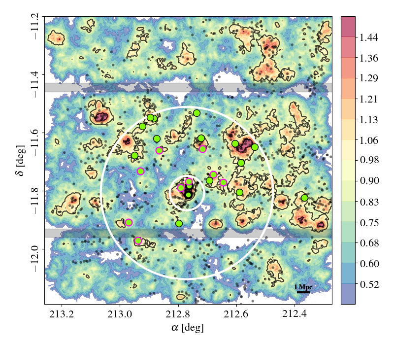
Figure 1: Density map of the CFHT/MEGACAM 1$\degr\times$1$\degr$ field around CL1411.1$-$1148. The colour-coding indicates the $\log_{10}$ of the density of galaxies averaged over the ten nearest neighbours. Black contours are at 1 and $3\sigma$ above the field mean density. The grey points identify all galaxies with a $z_{\mathrm{spec}}$ within $\mathrm{5\sigma_{cl}}$ of the cluster redshift. The inner and outer white circles are positioned at $R_{200}$ and $5R_{200}$ radius, respectively. The grey bands indicate the gaps between the MEGACAM CCDs. The green circles show our ALMA targets. The thick black outline identifies the two cluster members detected at 24 $\mu$m by Spitzer. The pink outer rings show the position of the galaxies with low gas fraction (see Fig. 9 and Sect. 4.2).

Figure 1 shows the galaxy density map in the 1$\degr\times$1$\degr$ region centred on CL1411.1$-$1148. Densities are calculated within a photometric redshift slice of $\pm(1+z_{cl})\times\sigma_{\rm NMAD}$ = 0.0547 around the cluster redshift. Within this photometric redshift slice, we use a ‘nearest neighbour’ approach, in which for any point $(x,y)$ the distance $r_{N}(x,y)$ to the $N{th}$ nearest neighbour is estimated. The galaxy density is thus the ratio between $N$ (fixed) and the surface defined by the adaptive distance: $\rho_{N}(x,y)=\frac{N}{\pi r^{2}_{N}(x,y)}$. We chose $N=10$, which corresponds to an average spatial scale (i.e. the mean distance between the ten galaxies) of about 0.8 Mpc, with 90% of the values being smaller than $\sim$1.5 Mpc. We selected 27 star-forming galaxies, satisfying the three criteria detailed above, and mapping the variety of local densities encountered inside and around the cluster as they appear from the photometric redshift estimates.

Figure 2 provides another 2D view of the spatial distribution of our ALMA targets over the same 1$\degr\times$1$\degr$ MEGACAM field of view. The galaxy positions are calculated relative to the position of the brightest cluster galaxy (BCG) in redshift and right ascension (RA). The galaxy relative position in redshift, $\Delta d_{\rm cl}$, is computed by taking the difference between the comoving distances of the galaxy and the BCG. The relative position in RA, $\Delta$RA, is obtained by transforming the angular separation between the BCG and the galaxy into a distance, using the angular distance at the redshift of the galaxy. Our full spectroscopic sample within $\pm$ $\mathrm{3\times\sigma_{cl}}$ of $z_{\rm cl}$ is presented, as are the photometric redshift cluster member candidates. The finger-of-God structure due to the relative velocities of the CL1411.1$-$1148 galaxies is clearly seen along the $\Delta d_{\rm cl}$-axis. Many of our targets are located in LSS related to CL1411.1$-$1148, such as the one extending westward from the cluster centre and up to 30 Mpc behind it; a few are in more isolated (lower density) regions. The information on our targets are summarised in Table 1.

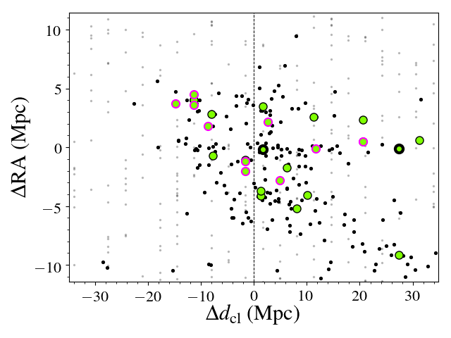
Figure 2: Light cone centred on $z_{\rm cl}=0.5195$ and extending to $\pm 3\sigma_{\rm cl}$ in redshift. In right ascension, $1\degr$ is covered. The vertical line corresponds to the cluster redshift. The grey points indicate the galaxies with a photometric redshift. Galaxies with spectroscopic redshifts are in black. Our sample is in green, lower $\mu_{\mathrm{H_{2}}}$ galaxies (see Sect. 4.2) are outlined in pink, and Spitzer observed galaxies are outlined in thick black. Distances are expressed relative to the brightest cluster galaxy (BCG).

PHIBSS2 encompasses 60 galaxies with CO(2-1) detections at $0.49\leq z\leq 0.8$, with stellar masses (M_star) higher than $10^{10.1}$ M_☉ and SFRs above 3.5 M_☉yr^-1 selected from the COSMOS, AEGIS and GOODS-North deep fields. A subsample of 19 systems falls at $0.49\leq z\leq 0.6$ and is used as comparison sample for our study.

Figure 3 presents the distribution of the $0.49\leq z\leq 0.6$ PHIBSS2 field galaxies and our ALMA sample in the $g-i$ versus $i$ colour–magnitude diagram (CMD). The position of the red sequence of CL1411.1$-$1148 is derived by considering the initial galaxy sample of EDisCS in the centre of CL1411.1$-$1148, for which we have $V$- and $I$- as well as $g$- and $i$-band photometry. We first identify the passive galaxies in the ($V$, $I$) CMD from De Lucia et al. (2007). This provides us with their positions in the ($g$, $i$) plane and allows us to fit the corresponding mean locus of the red sequence, and place its $\pm 0.3$ mag dispersion.

The $g$- and $i$-band photometry for the PHIBSS2 galaxies comes from the original CFHT Legacy survey catalogue for the COSMOS and AEGIS fields (Erben et al. 2009), while they were derived from $B$, $V$, and $I$ for the galaxies in the GOODS-North field from the 3D-HST catalogues (Capak et al. 2004). The latter may suffer from some uncertainties as no proper photometric calibration between these bands and $g$ and $i$ exists for galaxies.

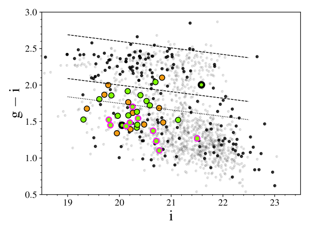
Figure 3: Observed colour–magnitude diagram, $g-i$ as a function of $i$ for the CL1411 galaxies. Our ALMA sample is in green. The dots with the thick black borders are our Spitzer-observed galaxies, and those with the pink borders are our low-$\mu_{\mathrm{H_{2}}}$ sample (see Sect. 4.3). The orange dots are the PHIBSS2 galaxies. The grey points are the photometric redshift members. The small black dots are the spectroscopic redshift galaxies, within $3\sigma_{\rm cl}$ of the cluster redshift. The dashed lines delimit the red sequence and its $\pm$0.3 mag dispersion. The dotted line delimits the transition zone between the blue clump and the red sequence, 0.25 mag below the lower boundary of the red sequence.

Figure 4 presents the rest-frame $U-V$ versus $V-J$ colour–colour diagram (CCD) that helps discriminate between passive and star-forming galaxies (Williams et al. 2009). The rest-frame colours were derived with EAZY (Brammer et al. 2008). We used the Johnson-Cousins $U$ and $V$ bands, and the 2MASS $J$ band (Skrutskie et al. 2006), together with a set of six templates: five main component templates obtained following the Blanton & Roweis (2007) algorithm and one for dusty galaxies (Brammer et al. 2008).

As expected, most of our targets fall in the star-forming region. Two systems, SEDCSJ1410249$-$1138157 and SEDCSJ1410518$-$1139195, are formally located within the passive region, however close to the boundary between the two regimes. None of them is located in the red sequence in Fig. 3, but rather in or close to the green valley, hence they are most likely transitioning to a quenched regime. On the other hand, the CO targets within the red sequences of the ($g$, $i$) CMD in Fig. 3 are not located in the passive region of the $UVJ$ plane, meaning that they are dusty.

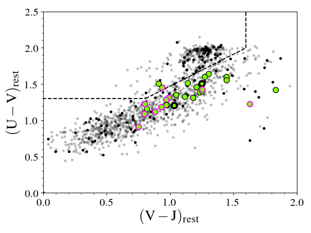
Figure 4: Rest-frame UVJ colour–colour diagram. The dashed lines separate passive galaxies, in the upper part, from star-forming galaxies (Williams et al. 2009). Colours and symbols are the same as in Fig. 3

Table 1: Sample properties: Galaxy ID, coordinates, optical spectroscopic redshift, and SED-based estimates of the galaxy $M_{\rm star}$ and SFRs

IDs	R.A. (J2000)	Dec (J2000)	${z_{\rm spec}}$	Mstar  ($\mathrm{10^{10}\,M_{\odot}}$)	$\mathrm{SFR}_{SED}$  ($\mathrm{M_{\odot}\,yr^{-1}}$)
SEDCSJ1409277$-$1149267	14:09:27.7553	$-$11:49:26.734	0.5275	$7.08^{+1.47}_{-1.47}$	$19.14^{+10.58}_{-11.90}$
SEDCSJ1410089$-$1138578	14:10:08.9192	$-$11:38:57.846	0.5217	$2.95^{+0.61}_{-0.68}$	$5.09^{+3.81}_{-3.52}$
SEDCSJ1410204$-$1142155	14:10:20.3750	$-$11:42:15.477	0.5199	$14.13^{+2.93}_{-3.58}$	$10.52^{+2.18}_{-7.63}$
SEDCSJ1410214$-$1148167	14:10:21.4016	$-$11:48:16.687	0.5226	$12.02^{+2.49}_{-2.21}$	$18.92^{+3.92}_{-9.59}$
SEDCSJ1410249$-$1138157	14:10:24.9817	$-$11:38:15.703	0.5199	$5.62^{+1.68}_{-2.07}$	$3.82^{+1.14}_{-2.99}$
SEDCSJ1410349$-$1146140†	14:10:34.9274	$-$11:46:14.071	0.5210	$3.09^{+0.64}_{-0.64}$	$5.71^{+2.70}_{-2.89}$
SEDCSJ1410429$-$1144385†	14:10:42.8737	$-$11:44:38.509	0.5308	$5.89^{+1.08}_{-1.08}$	$9.82^{+5.99}_{-4.18}$
SEDCSJ1410463$-$1145508	14:10:46.3146	$-$11:45:50.845	0.5214	$13.8^{+3.18}_{-2.22}$	$44.87^{+10.33}_{-40.30}$
SEDCSJ1410518$-$1139195†	14:10:51.8133	$-$11:39:19.548	0.5185	$4.9^{+0.79}_{-0.90}$	$3.33^{+1.65}_{-1.57}$
SEDCSJ1410532$-$1137091	14:10:53.2482	$-$11:37:09.091	0.5193	$4.68^{+0.97}_{-0.86}$	$15.38^{+10.63}_{-11.16}$
SEDCSJ1410568$-$1131594	14:10:56.8242	$-$11:31:59.398	0.5171	$5.5^{+1.64}_{-1.52}$	$6.27^{+1.88}_{-3.68}$
EDCSNJ1411028$-$1147006⋆	14:11:02.8248	$-$11:47:01.302	0.5202	$4.79^{+1.10}_{-0.99}$	$15.92^{+6.60}_{-7.88}$
SEDCSJ1411033$-$1146028†	14:11:03.2799	$-$11:46:02.789	0.5231	$1.82^{+0.50}_{-0.42}$	$4.59^{+1.27}_{-2.27}$
EDCSNJ1411036$-$1148506⋆	14:11:03.5909	$-$11:48:50.573	0.5282	$2.29^{+0.63}_{-0.58}$	$5.58^{+3.41}_{-3.28}$
SEDCSJ1411096$-$1147245†	14:11:09.6219	$-$11:47:24.523	0.5002	$0.74^{+0.22}_{-0.21}$	$2.86^{+0.84}_{-1.42}$
SEDCSJ1411112$-$1154452	14:11:11.2342	$-$11:54:45.236	0.5292	$10.72^{+2.22}_{-2.22}$	$16.29^{+3.38}_{-11.82}$
SEDCSJ1411243$-$1140510†	14:11:24.3255	$-$11:40:51.064	0.5171	$1.15^{+0.32}_{-0.27}$	$5.71^{+1.58}_{-1.84}$
SEDCSJ1411275$-$1139433†	14:11:27.5630	$-$11:39:43.290	0.5203	$3.39^{+0.70}_{-0.70}$	$10.89^{+2.26}_{-4.51}$
SEDCSJ1411296$-$1137130	14:11:29.6609	$-$11:37:13.061	0.5259	$5.5^{+1.39}_{-1.64}$	$4.65^{+1.18}_{-4.22}$
SEDCSJ1411319$-$1133048	14:11:31.9412	$-$11:33:04.781	0.5231	$3.31^{+0.76}_{-0.61}$	$7.62^{+4.30}_{-3.33}$
SEDCSJ1411348$-$1132522	14:11:34.7740	$-$11:32:52.216	0.5172	$4.9^{+1.01}_{-0.90}$	$8.85^{+8.66}_{-7.54}$
SEDCSJ1411416$-$1134421	14:11:41.6397	$-$11:34:42.092	0.5198	$5.13^{+0.94}_{-1.06}$	$7.53^{+4.94}_{-3.56}$
SEDCSJ1411431$-$1143589†	14:11:43.0675	$-$11:43:58.969	0.5156	$1.82^{+0.42}_{-0.34}$	$6.19^{+1.43}_{-2.71}$
SEDCSJ1411449$-$1158184†	14:11:44.9883	$-$11:58:18.447	0.5149	$5.75^{+1.59}_{-1.72}$	$12.79^{+3.54}_{-7.51}$
SEDCSJ1411478$-$1140389	14:11:47.7871	$-$11:40:38.956	0.5159	$2.51^{+0.46}_{-0.35}$	$10.64^{+10.78}_{-6.98}$
SEDCSJ1411480$-$1148562	14:11:47.9664	$-$11:48:56.199	0.5156	$11.22^{+2.07}_{-2.33}$	$9.38^{+8.1}_{-5.5}$
SEDCSJ1411528$-$1154286†	14:11:52.8004	$-$11:54:28.643	0.5160	$3.63^{+0.75}_{-0.67}$	$6.12^{+4.23}_{-2.96}$

2.2 ALMA observations

Fluxes in the CO(3-2) line, falling at $\sim$226 GHz in the ALMA Band 6 for $z\sim$ 0.52, were acquired during the ALMA Cycles 3 and 5 (programs 2015.1.01324.S, 2017.1.00257.S). The observations were conducted in the compact configurations C36$-$2 and C36$-$3, with 38 to 42 antennas, and C43$-$2, with 45 to 50 antennas, in Cycle 3 and 5, respectively. This led to beam sizes of 0.94″$\times$ 0.89″ and 1.2″$\times$ 0.95″ for Cycle 3 and 5, respectively. The integration times were of 7.5 hours (11 hours with overheads) in the 225.51–228.86 GHz spectral window. The resulting rms noise ranges from 0.09 to 0.25 mJy/beam in both cycles, and the spectral resolution is 50.7 km s^-1 for Cycle 3 and between 10.3 and 41 km s^-1 for Cycle 5, depending on the binning applied to reach sufficient signal-to-noise ratio.

A standard data reduction was performed with the CASA ALMA Science Pipeline (McMullin et al. 2007).The problematic antennas and runs were flagged. The continuum was fitted over the entire spectral window, except for the channels corresponding to the CO line, and subtracted. The final datacubes were created with the tclean routine using a Briggs weighting and a robustness parameter of 0.5, which is a trade-off between uniform and natural weighting. Finally we performed a primary beam correction, with the impbcor routine to obtain an astronomically correct image of the sky.

The final continuum-subtracted and primary-beam-corrected maps were exported to be analysed using GILDAS. The i-band images of our targets, the CO maps and spectra are shown in Fig. 12.

3 Derived parameters

3.1 CO flux and molecular gas mass

Fluxes, $S_{\mathrm{CO}}\,\Delta V$, were obtained by selecting the velocity window centred on the peak emission and maximising the flux over it and the spatial extent of the source.

Following Lamperti et al. (2020), the error on the flux is defined as

$$\epsilon_{\rm CO}=\frac{\sigma_{\rm CO}\Delta V}{\sqrt{\Delta V\Delta w_{ch}^{-1}}},$$ (1)

where $\sigma_{\rm CO}$ is the rms noise (in Jy) calculated in units of spectral resolution $\Delta w_{ch}$, and $\Delta V$ (in km s^-1) is the width of the spectral window in which the line flux is calculated, $\Delta w_{ch}=50.7$ km s^-1 for Cycle 3 and $\Delta w_{ch}=\{10.3;20.6;41\}$ km s^-1, depending on the binning applied to the spectrum, for Cycle 5. All intensity maps and integrated spectra are shown in Fig 12 of the Appendix. A few of our targets show double-peaked emission lines, which is an indication of rotation. This will be analysed in a forthcoming paper.

The intrinsic CO luminosity associated with a transition between the levels $J$ and $J-1$ is expressed as

$$L^{\prime}_{\mathrm{CO(J\rightarrow J-1)}}=3.25\times 10^{7}S_{\mathrm{CO(J\rightarrow J-1)}}\Delta V\,\nu_{\mathrm{obs}}^{-2}\,D_{\mathrm{L}}^{2}\,(1+z)^{-3},$$ (2)

where $L^{\prime}_{\mathrm{CO(J\rightarrow J-1)}}$ is the line luminosity expressed in units of ${\rm K\,km\,s\textsuperscript{-1}pc^{2}}$; $S_{\mathrm{CO(J\rightarrow J-1)}}\Delta V$ is the velocity-integrated flux in ${\rm Jy\,km\,s^{-1}}$; $\nu_{\mathrm{obs}}$ is the observed frequency in GHz; $D_{\mathrm{L}}$ is the luminosity distance in Mpc; and $z$ is the redshift of the observed galaxy (Solomon et al. 1997; Solomon & Vanden Bout 2005).

The total cold molecular gas mass (M${}_{\mathrm{H_{2}}}$) is then estimated as

$$M_{\mathrm{H_{2}}}=\alpha_{\mathrm{CO}}\frac{L^{\prime}_{\mathrm{CO(J\rightarrow J-1)}}}{r_{J1}},$$ (3)

where $\alpha_{\mathrm{CO}}$ is the CO(1-0) luminosity-to-molecular-gas-mass conversion factor, considering a 36% correction to account for interstellar helium, and $r_{J1}=L^{\prime}_{\mathrm{CO(J\rightarrow J-1)}}/L^{\prime}_{\mathrm{CO(1-0)}}$ the corresponding line luminosity ratio.

The $\alpha_{\mathrm{CO}}$ factor depends on different parameters: the average cloud density, the Rayleigh-Jeans brightness temperature of the CO transition, and the metallicity of the giant molecular clouds (GMCs) of the galaxy (Leroy et al. 2011; Genzel et al. 2012; Bolatto et al. 2013; Sandstrom et al. 2013). In the Milky Way, in nearby main-sequence (MS) star-forming galaxies, and in low-metallicity galaxies different methods are used to estimate this conversion factor. They converge to $\alpha_{\mathrm{CO}}=4.36\pm 0.9\,M_{\odot}\,{\rm(K\,km\,s^{-1}\,pc^{2})^{-1}}$, including the correction for helium, as a good estimate for normal star-forming galaxies (Dame et al. 2001; Grenier et al. 2005; Abdo et al. 2010; Leroy et al. 2011; Bolatto et al. 2013; Carleton et al. 2017).

The values of $r_{31}$ have been measured in a number of ways in nearby galaxies, and range from $\sim$ 0.2 to 2 (rarely reached however) (Mauersberger et al. 1999; Mao et al. 2010; Wilson et al. 2012). Dumke et al. (2001) found that $r_{31}$ could vary within a galaxy from $r_{31}\sim 0.8$ in the bulge to $r_{31}\sim 0.4$ in the disk for local galaxies without enhanced star formation. More recently Lamperti et al. (2020) identified a trend of $r_{31}$ with star formation efficiency, from $\sim$ 0.2 to 1.2 (with a mean value around 0.5), and inferred from modelling that the gas density is the main parameter responsible for this variation. At intermediate ($z\sim 0.5$) and high redshifts ($z\sim 1.5$), several studies assumed $r_{31}=0.5\pm 0.05$, as we do here as a fair compromise between all studies (Bauermeister et al. 2013b; Genzel et al. 2015; Chapman et al. 2015; Carleton et al. 2017; Tacconi et al. 2018). We discuss the impact of the choice of $\alpha_{\mathrm{CO}}$ and $r_{31}$ on the cold molecular gas masses of our galaxies in Sect. 4.4.

The full widths at half maximum (FWHMs) are derived from single or double Gaussian fits of the CO emission lines. We obtain a median FWHM of 224 km s^-1 with a standard deviation of 101 km s^-1 for our entire ALMA sample, similarly to what is found for our range of stellar masses by Freundlich et al. (2019).

The intrinsic CO(3-2) luminosity $L^{\prime}_{\mathrm{CO(3-2)}}$, the line FWHM, the cold molecular gas mass M${}_{\mathrm{H_{2}}}$, the corresponding gas-to-stellar-mass ratio $\mu_{\rm H_{2}}={\rm M}_{\mathrm{H_{2}}}/$M_star, and the redshift of the CO emission of our sample galaxies are listed in Table 3.1. One galaxy, SEDCSJ1411096$-$1147245, exhibits a large difference between its optical and CO redshifts. This is due to its optical redshift being estimated from IMACS-LDP, with a precision $\sigma_{z}=0.007$ (Just et al. 2015). SEDCSJ1411096$-$1147245 was not in our initial list of targets for ALMA. It turned out that while our primary target was not detected (SEDCSJ1411098$-$1147242 at $z_{\rm spec}=0.5260$), its companion galaxy within 3″, SEDCSJ1411096$-$1147245 was. This is shown in Fig. 12 in the $i$-band image; the original target is shown on the left.

Table 2: CO redshift, line-integrated flux, line width, luminosity of the CO(3-2) emission, cold molecular gas masses and cold molecular gas-to-stellar mass ratios of the ALMA targets.

IDs	$z_{\mathrm{CO}}$	$S_{\mathrm{CO(3-2)}}\Delta V$
	FWHM	($\mathrm{Jy\,km\,s^{-1}}$)
	$L^{{}^{\prime}}_{\mathrm{CO(3-2)}}$
	M${}_{\mathrm{H_{2}}}$
	$\mu_{\mathrm{H_{2}}}$
SEDCSJ1409277$-$1149267	0.5287	0.943 $\pm$ 0.052	568 $\pm$ 45	15.36 $\pm$ 0.853	13.39 $\pm$ 3.16	$0.189^{+0.084}_{-0.084}$
SEDCSJ1410089$-$1138578	0.5227	0.494 $\pm$ 0.029	236 $\pm$ 19	7.859 $\pm$ 0.457	6.85 $\pm$ 1.62	$0.232^{+0.103}_{-0.108}$
SEDCSJ1410204$-$1142155	0.5200	0.655 $\pm$ 0.021	110 $\pm$ 45	10.326 $\pm$ 0.329	9.0 $\pm$ 2.09	$0.064^{+0.028}_{-0.031}$
SEDCSJ1410214$-$1148167	0.5226	0.500 $\pm$ 0.008	93 $\pm$ 2	7.966 $\pm$ 0.132	6.95 $\pm$ 1.6	$0.058^{+0.025}_{-0.024}$
SEDCSJ1410249$-$1138157	0.5199	0.327 $\pm$ 0.015	262 $\pm$ 10	5.154 $\pm$ 0.243	4.49 $\pm$ 1.05	$0.08^{+0.043}_{-0.048}$
SEDCSJ1410349$-$1146140†	0.5213	0.164 $\pm$ 0.014	224 $\pm$ 21	2.597 $\pm$ 0.225	2.26 $\pm$ 0.56	$0.073^{+0.033}_{-0.033}$
SEDCSJ1410429$-$1144385†	0.5220	0.214 $\pm$ 0.018	118 $\pm$ 20	3.374 $\pm$ 0.288	2.94 $\pm$ 0.72	$0.050^{+0.021}_{-0.021}$
SEDCSJ1410463$-$1145508	0.5215	2.150 $\pm$ 0.010	206 $\pm$ 2	34.094 $\pm$ 0.199	29.73 $\pm$ 6.82	$0.215^{+0.099}_{-0.084}$
SEDCSJ1410518$-$1139195†	0.5193	0.175 $\pm$ 0.025	166 $\pm$ 31	2.750 $\pm$ 0.400	2.4 $\pm$ 0.65	$0.049^{+0.021}_{-0.022}$
SEDCSJ1410532$-$1137091	0.5213	1.398 $\pm$ 0.038	404 $\pm$ 12	22.03 $\pm$ 0.596	19.21 $\pm$ 4.44	$0.411^{+0.18}_{-0.17}$
SEDCSJ1410568$-$1131594	0.5172	0.483 $\pm$ 0.014	273 $\pm$ 9	7.53 $\pm$ 0.225	6.57 $\pm$ 1.52	$0.119^{+0.063}_{-0.061}$
EDCSNJ1411028$-$1147006	0.5207	0.884 $\pm$ 0.020	148 $\pm$ 6	13.95 $\pm$ 0.325	12.17 $\pm$ 2.80	$0.254^{+0.117}_{-0.111}$
SEDCSJ1411033$-$1146028†	0.5231	0.108 $\pm$ 0.010	243 $\pm$ 22	1.724 $\pm$ 0.155	1.5 $\pm$ 0.37	$0.083^{+0.043}_{-0.039}$
EDCSNJ1411036$-$1148506	0.5287	0.436 $\pm$ 0.049	148 $\pm$ 13	7.102 $\pm$ 0.799	6.19 $\pm$ 1.58	$0.270^{+0.144}_{-0.138}$
SEDCSJ1411096$-$1147245†	0.5259	0.144 $\pm$ 0.017	272 $\pm$ 72	2.306 $\pm$ 0.278	2.01 $\pm$ 0.52	$0.270^{+0.150}_{-0.145}$
SEDCSJ1411112$-$1154452	0.5292	0.602 $\pm$ 0.014	183 $\pm$ 11	9.843 $\pm$ 0.237	8.58 $\pm$ 1.98	$0.080^{+0.035}_{-0.035}$
SEDCSJ1411243$-$1140510†	0.5168	0.106 $\pm$ 0.006	183 $\pm$ 14	1.65 $\pm$ 0.098	1.44 $\pm$ 0.34	$0.125^{+0.064}_{-0.059}$
SEDCSJ1411275$-$1139433†	0.5203	0.154 $\pm$ 0.006	127 $\pm$ 5	2.431 $\pm$ 0.101	2.12 $\pm$ 0.49	$0.063^{+0.028}_{-0.028}$
SEDCSJ1411296$-$1137130	0.5259	0.411 $\pm$ 0.016	243 $\pm$ 27	6.634 $\pm$ 0.255	5.78 $\pm$ 1.35	$0.105^{+0.051}_{-0.056}$
SEDCSJ1411319$-$1133048	0.5233	0.736 $\pm$ 0.024	266 $\pm$ 13	11.75 $\pm$ 0.390	10.25 $\pm$ 2.37	$0.309^{+0.143}_{-0.129}$
SEDCSJ1411348$-$1132522	0.5173	0.645 $\pm$ 0.034	306 $\pm$ 27	10.05 $\pm$ 0.525	8.77 $\pm$ 2.06	$0.179^{+0.079}_{-0.075}$
SEDCSJ1411416$-$1134421	0.5200	0.759 $\pm$ 0.027	163 $\pm$ 6	11.97 $\pm$ 0.424	10.44 $\pm$ 2.42	$0.203^{+0.085}_{-0.089}$
SEDCSJ1411431$-$1143589†	0.5166	0.198 $\pm$ 0.008	124 $\pm$ 8	3.075 $\pm$ 0.124	2.68 $\pm$ 0.62	$0.147^{+0.068}_{-0.061}$
SEDCSJ1411449$-$1158184†	0.5149	0.259 $\pm$ 0.012	361 $\pm$ 17	4.002 $\pm$ 0.189	3.49 $\pm$ 0.82	$0.061^{+0.031}_{-0.032}$
SEDCSJ1411478$-$1140389	0.5160	0.450 $\pm$ 0.020	259 $\pm$ 29	6.984 $\pm$ 0.312	6.09 $\pm$ 1.42	$0.242^{+0.101}_{-0.090}$
SEDCSJ1411480$-$1148562	0.5160	0.388 $\pm$ 0.024	265 $\pm$ 34	6.021 $\pm$ 0.378	5.25 $\pm$ 1.25	$0.047^{+0.020}_{-0.021}$
SEDCSJ1411528$-$1154286†	0.5166	0.102 $\pm$ 0.023	166 $\pm$ 58	1.584 $\pm$ 0.362	1.38 $\pm$ 0.45	$0.038^{+0.020}_{-0.019}$

3.2 Stellar masses and star formation rates

The stellar masses and SFRs were derived with MAGPHYS (da Cunha et al. 2008) using the $u$, $g$, $r$, $i$, $z$, and Ks bands, as well as the 24 $\mu$m flux when available. The stellar populations and dust extinction models are those of Bruzual & Charlot (2003) and Charlot & Fall (2000). MAGPHYS provides probability density functions (PDFs) for each parameter (i.e. SFR, M_star, dust mass, dust temperature). For each quantity, we considered the peak value of the PDFs and our uncertainties correspond to the 68% confidence interval of the same PDFs. The wavelength coverage of our photometric bands does not allow the identification of AGNs, which could affect the SFR and M_star estimates. However, the analysis of the [OII]-to-H$\beta$ line ratio indicates that most likely the emission lines in our galaxy spectra are not typical of AGNs (Sánchez-Blázquez et al. 2009). This adds to our current understanding that there is a smaller percentage of AGNs in clusters (less than 3%) than in the field (Miller et al. 2003; Kauffmann et al. 2004; Mishra & Dai 2020).

We used the two galaxies in the core of CL1411.1$-$1148 which were detected by Spitzer at 24 $\mu$m to evaluate the robustness of our stellar mass and SFR estimates. The 24 $\mu$m flux (corresponding to $\sim$15$\mu$m at $z\sim 0.52$) allows us to better constrain the dust emission and judge its impact on the derived quantities. Figure 5 presents the spectral energy distribution (SED) fits and the corresponding likelihood distribution of M_star and SFR for EDCSNJ1411028$-$1147006 and EDCSNJ1411036$-$1148506. For both galaxies, M_star stays identical with or without the 24 $\mu$m flux. As to the SFR, the PDFs of EDCSNJ1411028$-$1147006 are essentially identical with or without the 24 $\mu$m flux point. The case of EDCSNJ1411036$-$1148506 is different. Its SFR PDF is wider without the 24 $\mu$m flux point (peak value at $\log({\rm SFR})=0.5$) than when calculated with the 24 $\mu$m point (peak value at $\log({\rm SFR})=0.8$). The two PDFs have medians within 0.3 dex and are highly overlapping, hence the SFR estimates are consistent with each other. EDCSNJ1411036$-$1148506 is the faintest galaxy in our sample in the $i$ band ($>$ 21.5, Fig. 3) and is probably observed edge-on, as seen in Fig. 12. Its UV flux is very low, with the deepest rest-frame 4000 Å break, hence representing the most challenging and dusty case in our sample.

In summary, our stellar mass estimates are robustly derived from $u$ to $K_{\rm s}$ photometry. As for the SFRs, missing the Spitzer 24 $\mu$m flux could lead to underestimated values, but our error bars are realistic enough to take this possibility into account.

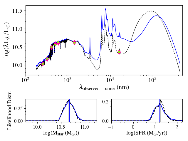
(a) EDCSNJ1411028$-$1147006.

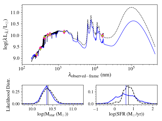
(b) EDCSNJ1411036$-$1148506.

Figure 5: SEDs and likelihood distributions for the two Spitzer-observed galaxies: EDCSNJ1411028$-$1147006 (a) and EDCSNJ1411036$-$1148506 (b). The blue curves are without the MIPS 24 $\mu$m fluxes and the black dashed curves are with the MIPS 24 $\mu$m fluxes. The top panels show the fitted SEDs in black and blue, the observed fluxes in green, and the model fluxes in pink. The bottom panels of (a) and (b) show the likelihood distributions for M_star and SFR, and the medians for the M_star and SFR, as the blue and black vertical lines, derived with MAGPHYS.

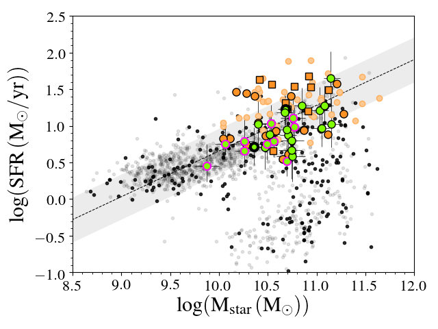
Figure 6: Location of the CL1411 (grey) and ALMA (green) galaxies in the stellar mass–SFR plane. The dots with thick black borders represent the Spitzer-observed galaxies and those with the pink outline indicate the low-$\mu_{\mathrm{H_{2}}}$ galaxies. Galaxies in black and grey are the rest of the spectroscopic and photometric samples, respectively, at the cluster redshift. The plain orange circles are the PHIBSS2 galaxies with $0.49\leq z\leq 0.6$, while the light orange circles trace the PHIBSS2 sample at $0.6<z\leq 0.8$; the orange squares show the cluster LIRGs of Castignani et al. (2020) at $z\sim 0.54$. The dashed black line is the Speagle et al. (2014) MS corrected for a Chabrier IMF, at our cluster redshift with the corresponding $\pm$0.3dex scatter as the grey shaded area.

Figure 6 presents the position of our sample galaxies relative to the MS of normal star-forming galaxies at the same redshift (Speagle et al. 2014), corrected for a Chabrier IMF. Our spectroscopic and photometric datasets are both displayed. More than three-quarters (78%) of our ALMA targets fall within the $\pm$ 0.3 dex dispersion of the MS. Three of our ALMA targets are located just below the $-0.3$ dex limit; however, they are still compatible with the MS considering the uncertainties on the SFRs. Three systems fall in between the MS and the red sequence. These are systems in the transition region between star-forming and passive systems. Mancini et al. (2019) show that this region of the stellar mass–SFR plane contains galaxies that are quenching, but also galaxies that are undergoing a rejuvenation of star formation. With the exception of three PHIBSS2 galaxies, which stand clearly above the MS, PHIBSS2 $z\sim 0.55$ systems and our ALMA targets cover the same SFR–M_star space. Their cold gas reservoirs can therefore be compared.

4 Discussion

4.1 Comparison sample

To place our results in a global context, our datasets are compared to the other CO-line observations available to date. They are listed below in order of increasing redshift.

• 53 detections of CO(1-0) for local ($0.001<z<0.05$) IR luminous galaxies (Gao & Solomon 2004);

• 19 detections of CO(1-0) for LIRGs with $z\sim 0.01$ (García-Burillo et al. 2012);

• 333 detections of CO(1-0) for galaxies from xCOLD GASS (Saintonge et al. 2017) with M${}_{\rm star}>10^{10}$M_⊙ and $z$ between 0.01 and 0.05;

• 46 detections of CO(3-2) for galaxies selected from the BASS survey (Baumgartner et al. 2013) with $z<0.04$ and studied in Lamperti et al. (2020);

• 27 detections of CO(1-0) and CO(3-2) for star-forming galaxies with $z$ from 0.06 to 0.3 from the EGNoG survey (Bauermeister et al. 2013a, b);

• 8 detections of CO(1-0) emission for galaxies selected based on their 4000 Å emission strength with redshifts from 0.1 to 0.23 (Morokuma-Matsui et al. 2015);

• 9 detections of CO(1-0) for star-forming galaxies inside and in the foreground and background of two Abell clusters, A2192 and A963, with $z$ between 0.13 and 0.23, from the COOL BUDHIES survey (Cybulski et al. 2016);

• 8 CO(1-0) and 12 CO(2-1) observations of LIRGs inside clusters with redshift between 0.21 and 0.56 (Castignani et al. 2020);

• 2 CO(2-1) and 1 CO(1-0) detections of LIRGS inside two clusters at $z=0.397$ and $0.489$ (Jablonka et al. 2013);

• 5 CO(1-0) detections from 24$\mu$m-selected galaxies at $z=0.4$ (Geach et al. 2009, 2011);

• 46 detections of CO(2-1) for star-forming galaxies with $0.5\leq z\leq 0.8$, as part of the PHIBSS2 survey (Tacconi et al. 2018; Freundlich et al. 2019);

• 4 CO(2-1) detections for massive and passive galaxies from the LEGA-C survey with $0.6\leq z\leq 0.73$ (Spilker et al. 2018);

• 52 detections of CO(3-2) for star-forming galaxies with redshifts ranging from 1 to 2.3, as part of the PHIBSS1 survey (Tacconi et al. 2010, 2013);

• 17 CO(2-1) detections of main-sequence galaxies inside the XMMXCS J2215.9$-$1738 cluster at $z=1.46$ (Hayashi et al. 2018);

• 5 detections of CO(2-1) for near-IR selected galaxies at $z\sim 1.5$ from Daddi et al. (2010);

• 11 detections of CO(2-1) emission for cluster galaxies at $z\sim 1.6$ from Noble et al. (2017, 2019);

• 2 detections of CO(1-0) emission of massive cluster galaxies at $z\sim 1.62$ from Rudnick et al. (2017)

It is noteworthy that most of these datasets are made of field galaxies, with the exception of Geach et al. (2009, 2011), Jablonka et al. (2013), Cybulski et al. (2016), Noble et al. (2017, 2019) and Castignani et al. (2020). Depending on the focus of the discussions below, we include all or only parts of this comparison sample. The PHIBSS2 galaxies at $0.49\leq z\leq 0.60$ are the best field counterparts to our study in terms of redshift range, and even more importantly because most of the galaxies are forming stars at a normal rate for their stellar masses. The ten galaxies of the MACS J0717.5+3745 cluster observed by Castignani et al. (2020) are, in redshift, the closest cluster galaxy counterparts to our study. However, they were selected differently, specifically as LIRGs, and consequently probe on average higher specific SFRs (sSFR = SFR/M_star) than our sample, and do not extend down to the lowest values as our sample does, as can be seen in Fig. 7. The three field PHIBSS2 galaxies with the highest gas fraction are systems very clearly above the MS, hence they do not have counterparts in our dataset. They are nonetheless included in our analysis.

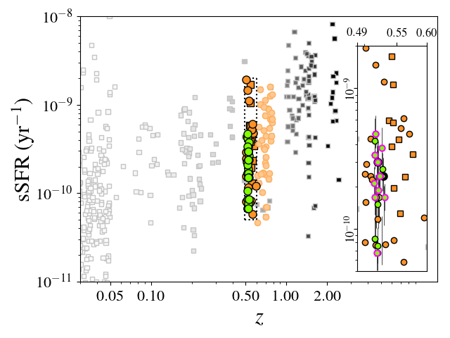
Figure 7: Specific star formation rates as a function of redshift. The green dots identify our ALMA targets; dots with the thick black borders are the galaxies detected at 24 $\mu$m, and dots with the pink outlines galaxies with low gas fraction. The orange circles stand for the PHIBSS2 galaxies, with the darker shade for the systems at $0.49\leq z\leq 0.6$ and the lighter for the galaxies at $0.6<z\leq 0.8$. The orange squares indicate the M0717 LIRGs. The symbols in shades of grey are for the samples we pulled from the literature at different redshifts. We provide a zoom-in of the region delineated by the dotted lines (see inset), around the redshift of CL1411.1$-$1148. While three of the PHIBSS2 sources have sSFRs well above those of our ALMA targets, the sSFRs of the rest of the PHIBSS2 sources are in perfect agreement with those from our sample.

4.2 Gas fractions

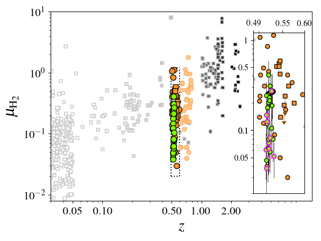
Figure 8: Molecular gas-to-stellar mass ratio as a function of redshift. The colour-coding is as in Fig. 7. We provide a zoom-in of the region delineated by the dotted lines (see inset), around the redshift of CL1411.1$-$1148.

Figure 8 shows the variation of the galaxy gas fraction, $\mu_{\mathrm{H_{2}}}$$={\rm M}_{\rm H_{2}}/$M_star, with redshift for both our targets and other CO-line measurements published to date. Our sample is the largest sample of galaxies with direct cold gas measurements at a single intermediate redshift ($0.5000<z<0.5375$) and the only one with galaxies in interconnected cosmic structures around a given galaxy cluster. The cluster galaxy sample of Castignani et al. (2020) at $z\sim 0.54$ extends to $\sim$ 1.6 times the virial radius of M0717, hence stays closer to the cluster centre than the present study.

We probe a wide range of $\mu_{\mathrm{H_{2}}}$ values, from $\sim$0.04 to 0.30; 44% of our galaxies have $\mu_{\mathrm{H_{2}}}$ lower than 0.1. This contrasts with the bulk of other datasets at $z>0.05$. Of these, only the PHIBSS2 sample at $0.49\leq z\leq 0.8$ has gas fractions that are as low as ours, and even then only $\sim$ 20% of the coeval PHIBSS2 galaxies have $\mu_{H_{2}}$ below 0.1. The low gas fractions we see in our sample compared to those in the field cannot simply be due to cosmic evolution in $\mu_{\mathrm{H_{2}}}$, as samples at both lower and higher redshift have increased gas fractions. It is more likely linked to how we selected our galaxies as many early CO studies that dominate the literature values tended to select LIRGs rather than normal star-forming galaxies. This could impact the derivation of the scaling relations using different studies covering a wide range of redshifts (e.g. Tacconi et al. 2018).

Figure 9: Fraction of cold molecular gas as a function of the galaxy stellar masses. The colours and shapes of the symbols are the same as in Fig. 7. The dotted line is the fit of the $M_{\rm star}$–$\mu_{\mathrm{H_{2}}}$ relation for the PHIBSS2 galaxies at $0.49<z\leq 0.6$, with its variance being represented by the two dashed lines. The pink outlined green symbols are for our low-$\mu_{\mathrm{H_{2}}}$ galaxies, which are located below the $1\times$ $\sigma_{\rm H_{2}}$ line of the M_star–$\mu_{\mathrm{H_{2}}}$ relation for the PHIBSS2 field galaxies.

Figure 9 presents the galaxy cold gas fractions as a function of their stellar masses. It constitutes the main result of our analysis. At redshifts similar to those of our sample, $0.49\leq z\leq 0.6$, the relation between $\mu_{\mathrm{H_{2}}}$ and M_star for the PHIBSS2 subsample has a slope of $\sim-0.82$ and a variance $\sigma_{\rm H_{2}}=0.37$ dex. A significant fraction of our targets fall below this 1 $\times$ $\sigma_{\rm H_{2}}$ line of the M_star–$\mu_{\mathrm{H_{2}}}$ relation for the field galaxies. This means that while 63% of the galaxies in the LSS of CL1411.1$-$1148 have gas mass fractions comparable to their field counterparts, 37% lie below the locus defined by field galaxies at the same stellar mass. We refer to these ten galaxies as low-$\mu_{\mathrm{H_{2}}}$ systems. In order to quantify the significance of this low-$\mu_{\mathrm{H_{2}}}$ population, we randomly extracted, 100 000 times, 27 galaxies from a normal distribution of sources with the same mean $\mu_{\mathrm{H_{2}}}$ and same standard deviation as PHIBSS2. The probability of getting 37% of the galaxies below 1$\sigma$ is less than 1%. Therefore, this excess to one side of the field relation deviates significantly from the expected tail of sources for a Gaussian distribution, and reveals a population that was absent from previous surveys. These galaxies are identified with the dagger symbol (^†) in the tables and they are highlighted in pink in all figures. Combining our sample with the comparison field PHIBSS2 subsample with $z\leq 0.6$, the relation between $\mu_{\mathrm{H_{2}}}$ and M_star becomes slightly shallower, with a slope of $-0.51$.

Interestingly, the SFRs of all but one (SEDCSJ1410518$-$1139195) of the low-$\mu_{\mathrm{H_{2}}}$ galaxies are normal for their stellar masses, indicating that their molecular gas reservoir, either in mass or in physical properties, is modified before their star formation activity is impacted. This possibility was also suggested by Jablonka et al. (2013) for LIRGs in clusters and by Alatalo et al. (2015) for local elliptical galaxies, who find that their diffuse gas reservoir could potentially be stripped before the dense gas, which is more closely related to star formation. This disconnection between $\mu_{\mathrm{H_{2}}}$ and SFR is further illustrated in Fig. 10 which presents $\mu_{\mathrm{H_{2}}}$ as a function of the galaxy sSFR, normalised to their position on the MS, following Genzel et al. (2015).

Figure 10: Fraction of cold molecular gas as a function of the normalised specific star formation rates. The colours and shapes of the symbols are the same as in Fig. 7. The dotted lines represent the $\pm 0.3$ dex scatter of the MS.

Although our galaxies have normal SFRs for their stellar masses, they have a significantly different distribution of gas fractions than the field samples. Our low-$\mu_{\mathrm{H_{2}}}$ targets populate a region that to date has remained uncovered at similar redshift, and reveal that there is a much larger scatter in $\mu_{\mathrm{H_{2}}}$ at fixed sSFR (nearly twice as much) than previously encountered in other studies at similar redshifts. To quantify this result, we performed an Anderson–Darling (A-D) test (Scholz & Stephens 1987) between the $\mu_{\mathrm{H_{2}}}$ distributions of PHIBSS2 galaxies and ALMA targets, both within the MS. The A-D test is more sensitive to differences in the tails of the distributions than a Kolmogorov–Smirnov test. When all MS galaxies are considered, the A-D test results in p = 0.027, meaning that there is only a 2.7% chance that the two samples come from the same distribution in $\mu_{\mathrm{H_{2}}}$. When we restrict the comparison to the low-$\mu_{\mathrm{H_{2}}}$ MS galaxies only and the full MS PHIBSS2 galaxies, we find p = $1.3\times 10^{-3}$, which clearly shows that this low-$\mu_{\mathrm{H_{2}}}$ tail of the ALMA sample comes from a significantly different $\mu_{\mathrm{H_{2}}}$ distribution ($>$99%) from that of the PHIBSS2 MS galaxies.

Figure 11: Dependence of the depletion timescale (in Gyr) as a function of the normalised specific star formation rates. The colours and shapes of the markers are the same as in Fig. 7. The horizontal dotted line is located at 1 Gyr and the vertical dotted lines represent the $\pm$ 0.3 dex scatter of the MS.

Figure 11 shows the depletion timescales (M_gas/SFR) as a function of the normalised sSFR. Our low-$\mu_{\mathrm{H_{2}}}$ galaxies have short depletion times $\sim 300$ Myr compared to the bulk of the population known so far. This implies that they should consume their gas and quench more rapidly.

4.3 Link with local density

As a first attempt to link the spatial location of our sample galaxies and their gas masses, we searched for a possible correlations between the galaxy gas fraction and cluster-centric distance, but did not find any.

We then looked into the possibility that low gas fractions correlate with local (over)densities. Figures 1 and 2 suggest that while the low-$\mu_{\mathrm{H_{2}}}$ galaxies are embedded in coherent LSS, their relation with a local and/or small-scale environment does not stand out. Hence, there must be more than one parameter explaining the status of the galaxy gas reservoir that we are witnessing.

Similarly, we have looked into the environment of the PHIBSS2 galaxies. For the galaxies in the COSMOS field, we used the G10-COSMOS catalogue (Davies et al. 2015) for their position and redshift, and the zCOSMOS 20k group catalogue (Knobel et al. 2012). The 3D-HST survey catalogue (Brammer et al. 2012; Skelton et al. 2014; Momcheva et al. 2015) was used for the PHIBSS2 galaxies within the AEGIS and GOODS-North fields. We used the DEEP2 group catalogue (Gerke et al. 2012) for AEGIS. No equivalent group catalogue was found for GOODS-North. Among the 19 PHIBSS2 galaxies, only 5 belong to a group or are close to one. However, we did not find any correlation between their gas content and the density of their local environment.

4.4 Caveats

The derivation of cold gas masses involves two parameters, $\alpha_{\mathrm{CO}}$ and $r_{31}$. This raises the question of whether the low-$\mu_{\mathrm{H_{2}}}$ galaxies could arise from our choices of these parameters.

The PHIBSS2 CO conversion factor, $\alpha_{\mathrm{CO}}$, decreases with increasing metallicity, from 4.7 down to 3.8 $\,M_{\odot}\,{\rm(K\,km\,s^{-1}\,pc^{2})^{-1}}$. Applying the same definition and estimating the metallicity from its relation with the galaxy stellar mass as in Genzel et al. (2012), $\alpha_{\mathrm{CO}}$ could in principle vary from $\alpha_{\rm CO}=3.76$ to $4.91\,M_{\sun}\,{\rm(K\,km\,s^{-1}\,pc^{2})^{-1}}$ over our range of masses. This would increase by 12% the cold molecular gas mass of the two lowest mass galaxies (M${}_{\rm star}\lesssim 10^{10}\,M_{\sun}$) in our sample, keep galaxies at M${}_{\rm star}\sim 10^{10}\,M_{\sun}$ at the same positions, and decrease by 13% the gas masses of the most massive of our target. None of these shifts would change the identification of the low-$\mu_{\mathrm{H_{2}}}$ galaxies.

As to the flux ratios, the observations of PHIBSS2 were conducted in CO(2-1), with $r_{21}=0.77$ as a trade off between the values found in earlier studies, which range from 1 to 0.6 (Freundlich et al. 2019). As seen from Eq. 3, increasing $r_{31}$ decreases the galaxy gas mass, hence increasing the gas mass in our low-$\mu_{\mathrm{H_{2}}}$ galaxies is not an option. As shown in previous studies of nearby galaxies (Mauersberger et al. 1999; Mao et al. 2010; Lamperti et al. 2020), there is a large scatter in $r_{31}$ ($\sim$0.1) with any fixed parameter involving the galaxy SFRs. It should be noted, however, that these nearby samples are mostly composed of galaxies above the main sequence unlike our targets. The value of $r_{31}$ would need to be decreased by at least a factor 2 in order to reconcile our sample with the PHIBSS2 galaxies in Fig. 9. At the lowest tail of the distribution $r_{31}=0.2$ is rarely encountered (Mao et al. 2010). Moreover, if $r_{31}$ does vary from one galaxy to another, some normal systems could have $r_{31}$ higher than 0.5. Hence, they would potentially move into the low-$\mu_{\mathrm{H_{2}}}$ region. This issue definitely needs further observations directly in CO(1-0).

5 Conclusion

We have presented the CO(3-2) emission line fluxes obtained with ALMA for a sample of 27 galaxies located within $5\times R_{200}$ of the centre of the EDisCS cluster CL1411.1$-$1148 at $z=0.5195$. This constitutes the largest sample of galaxies with direct cold gas measurements at a single intermediate redshift ($0.5000<z<0.5375$), and the only sample of galaxies in interconnected cosmic structures around a galaxy cluster.

Unlike most of the previous studies which targeted galaxies based on their SFRs, our selection is based on stellar masses and on ground-based photometry in the $u,\,g$, and $i$ bands only, with the requirement that galaxies are in the blue cloud of the cluster colour–magnitude diagrams, and have available spectroscopic redshifts. The derivation of the galaxy stellar masses and star formation rates placed all but two of our targets on the MS of the normal star-forming galaxies, with stellar masses between log(M_star/M${}_{\sun})=9.8$ and 11.2, and SFRs ranging from $\log({\rm SFR}/($M${}_{\sun}{\rm yr}^{-1}))=0.3$ up to 1.7. Two galaxies fall within the passive region of the rest-frame $UVJ$ colour–colour diagram. They still are very close to the star-forming sequence, which suggests that these systems are transitioning to a quenched state.

Our sample covers a wide range of cold molecular gas masses, from $1.38\times 10^{9}$ up to $3\times 10^{10}$ M_☉. The low tail of this gas mass distribution probes lower values than most other studies of CO at $z>0.05$. We have compared our results to the PHIBSS2 survey (Freundlich et al. 2019), which is the best field counterpart to our study at $z\sim 0.5$. Looking at the link between galaxy gas fraction and stellar mass, we find that while 63% of our galaxies follow the same trend between $\mu_{\mathrm{H_{2}}}$ and M_star as field galaxies, 37% of our targets fall below the 1$\sigma$ variance of the relation derived for the field galaxies. This excess to one side of the field relation deviates significantly from the expected tail of sources for a Gaussian distribution and reveals a population that was absent from other surveys. Our cold molecular gas mass estimates depend on our choice of the CO conversion factor, $\alpha_{\mathrm{CO}}$, and the line ratio, $r_{31}$. But our results remain the same for all reasonable values of these parameters. Nevertheless direct observation of the CO(1-0) transition should help shed definitive light on this issue.

Interestingly, the SFRs of the low-$\mu_{\mathrm{H_{2}}}$ galaxies are normal for their stellar masses. This indicates that their molecular gas reservoir changes, either in mass or properties, before the galaxy SF activity is impacted. Our sample displays a much larger scatter in $\mu_{\mathrm{H_{2}}}$ than previously encountered in other studies at similar redshifts (at least two times larger). This is the case at fixed SF activity and stellar mass, as represented by the specific SFR normalised to the position of the galaxies on the mass sequence.

Although our galaxies have been selected in the vicinity of a galaxy cluster, we have not identified any correspondence between the low gas fraction of the galaxies and the local density of their environment.

Appendix A ALMA maps and spectra of our galaxies

In this appendix we present the $i$-band images, the ALMA intensity maps, and the spectra of all of our targets. The low-$\mu_{\mathrm{H_{2}}}$ targets are indicated as such by a label at the bottom left of the $i$-band image.

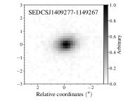
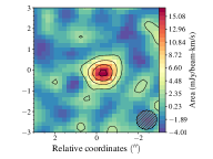
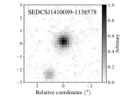
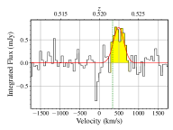
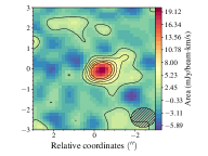
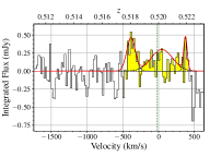
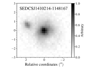
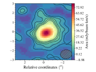
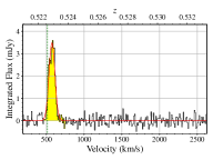
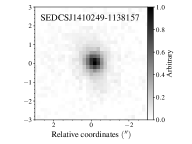
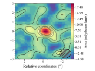
Figure 12: Left: CFHT/MEGACAM i-band images of our galaxies, unless stated otherwise, in a $6\arcsec\times 6\arcsec$ snapshot, centred on the galaxies coordinates. Middle: ALMA map of the CO(3-2) emission around our galaxies. Spatial scale is the same as in the left panel. The colour wedge of the intensity map is in mJy$/$beam km s^-1. The contours are defined such that they are spaced by 2 times the rms starting at 1 time above the rms. In the bottom right corner is the beam size. Right: The spectrum shows the flux, $S_{\mathrm{CO}}$, spatially integrated as indicated in Sect. 2.2, of the source in mJy in function of the velocity in km s^-1, with respect to a fixed frequency. The Gaussian profiles are fits of the emission lines from which we derived our FWHMs. The yellow filled zones correspond to the spectral extent of the emissions. The green vertical line corresponds to the spectroscopic redshift.

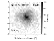
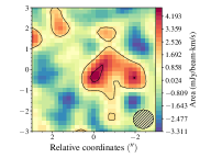
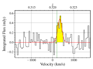
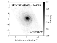
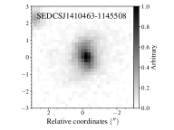
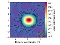
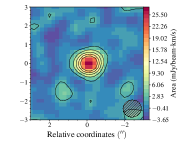
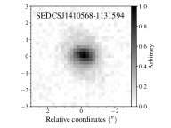
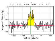
Figure 13: Continued.

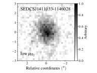
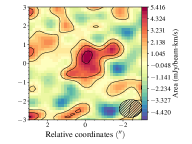
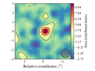
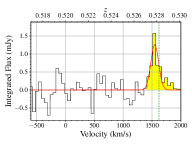
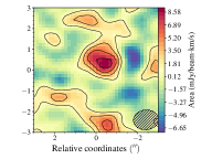
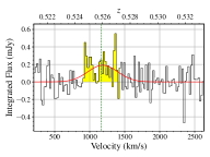
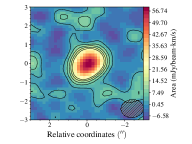
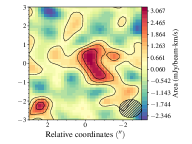
Figure 14: Continued.

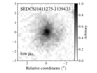
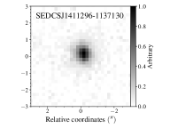
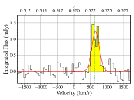
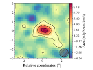
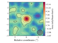
Figure 15: Continued.

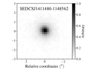
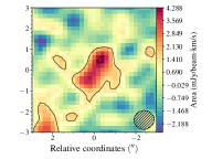
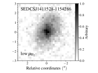
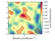
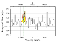
Figure 16: Continued.