Using the Gini coefficient to characterize the shape
of computational chemistry error distributions
Abstract
The distribution of errors is a central object in the assesment and benchmarking of computational chemistry methods. The popular and often blind use of the mean unsigned error as a benchmarking statistic leads to ignore distributions features that impact the reliability of the tested methods. We explore how the Gini coefficient offers a global representation of the errors distribution, but, except for extreme values, does not enable an unambiguous diagnostic. We propose to relieve the ambiguity by applying the Gini coefficient to mode-centered error distributions. This version can usefully complement benchmarking statistics and alert on error sets with potentially problematic shapes.
1 Introduction
The reliability of a computational chemistry method is conditioned by the distribution of its prediction errors. Distributions with heavy tails elicit a risk of large prediction errors. As a benchmarking statistic, the popular mean unsigned error (MUE) bears no information on such a risk [1, 2, 3, 4]. We have recently reported a case where two unbiased error distributions with identical values of the MUE present widely different risks of large errors because of heavy tails in one of them [5, 4]. It would therefore be very useful to complement the MUE with a statistic indicating or quantifying the risk of large errors.
We recently proposed alternative statistics such as [2], , [2] and systematic improvement probability (SIP) [3]. In terms of risk, these statistics offer the following interpretations:
-
•
There is a 5 % risk for absolute errors to exceed .
-
•
There is a probability that absolute errors are larger than a chosen threshold . provides a direct quantification of the risk of large errors, but has to be defined a priori and might be user-dependent, which complicates its reporting in benchmarking studies.
-
•
For two methods and , the SIP provides the system-wise probability that the absolute errors of are smaller than the absolute errors of , informing on the risk incurred by switching between two methods. Interestingly, the SIP analysis provides a decomposition of the MUE difference between two methods in terms of gain and loss probabilities [3].
The and partly answer the question, but they are point estimates on the cumulated density function of the absolute errors, and a statistic accounting for the whole distribution might be of interest. Besides, it is well established in econometrics that measures of dispersions such as the variance perform poorly at risk estimation and that higher moments of the distributions have to be considered [6]. This would lead us to such measures as skewness and kurtosis, but none of these alone would be able to cover all the scenarii. The risk of large errors through heavy tails of the errors distribution might be associated with large skewness or large kurtosis or a combination of them.
The Lorenz curve [7] is widely used in econometrics to represent the distribution of wealth in human populations. Its summary statistics, notably the Gini coefficient (noted ) [8, 9, 10], are used to evaluate the degree of inequality within these populations. The Gini coefficient is also used, for instance, in ecology, to estimate the inequality of properties within plant populations [11, 9], in astronomy, to characterize the morphology of galaxies [12], or in information theory, to characterize the sparsity of datasets [13].
The Lorenz curve has many mathematical representations, the most interesting one, for us, being its formulation as an integral of the quantile function, a direct link with our study of probabilistic metrics [2, 3, 4]. More precisely, we explore here the interest of the Gini coefficient as a complement to the MUE in benchmarking studies.
We introduce the statistical tools and their implementation in Section 2, and apply them to a series of datasets to illustrate the interest and limitations of the Gini coefficient in Section 4. An adaptation of the Gini coefficient is proposed to relieve its main drawbacks when applied to error datasets.
2 Statistical methods
2.1 Definitions
Let us consider a distribution of errors with probability density function (PDF) . The absolute errors have a folded PDF . To avoid ambiguity, statistics based on absolute errors are indexed by .
2.1.1 CDF and quantile function
The cumulative distribution function (CDF) of the absolute errors is noted
| (1) |
from which the quantile function is the inverse
| (2) |
2.1.2 Mean unsigned error
The mean unsigned error (MUE), is defined as
| (3) |
Using the change of variable , and , the MUE also can be shown to be the integral of the quantile function
| (4) | ||||
| (5) |
2.1.3 The Lorenz curve
The Lorenz curve gives the percentage of cumulated absolute errors due to the % smallest values, or equivalently, the portion of the MUE due to the % smallest absolute errors:
| (6) |
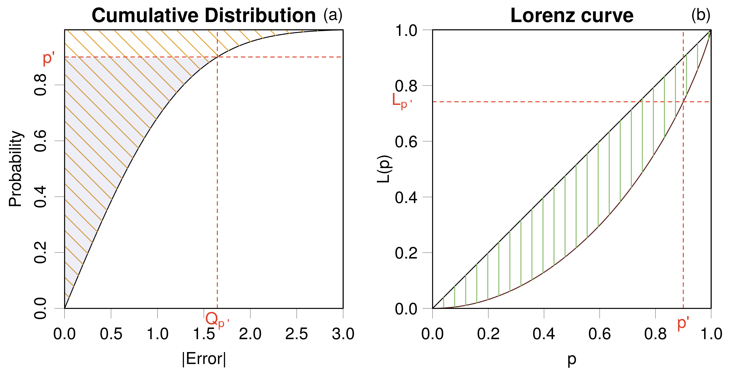
As shown in Fig. 1(a), it is the ratio between the slanted shaded area and the total slanted area. Its value for is reported on the corresponding Lorenz curve graph (Fig. 1(b)).
The Lorenz curve provides a scale-invariant representation of the CDF [14], with the following properties: is concave, increasing with , such as , and . lies one the identity line () when all the errors are equal, i.e. . Note that this case corresponds to a discontinuous CDF, with a jump at . The deviation of an error distribution from this extreme case can be measured by the Gini coefficient.
2.1.4 The Gini coefficient
It is related to the area between and the identity line (Fig. 1(b))
| (7) |
where the factor two is used to scale between 0 and 1. The smaller , the closer the Lorenz curve to the identity line. The Gini coefficient, usually noted , is generally used for distributions with positive support. Our notation is a reminder that we are working here with distributions of absolute errors .
For sets of absolute errors with a normal distribution , is proportional to the coefficient of variation [11], where the standard deviation of the absolute errors
| (8) |
Note that this relationship does hold only when all errors are of the same sign (), therefore with small values.
Two typical values of will be useful in the following:
-
•
for any zero-centered normal distribution of errors , the distribution of absolute errors is the half-normal distribution, with value [15];
-
•
for any zero-centered uniform distribution, , or any uniform distribution with a bound at zero, or , folding produces a uniform distribution with the minimal bound at zero, with value [15].
2.1.5 Skewness and kurtosis
Skewness measures the asymmetry of a distribution, while kurtosis is used as a measure either of its “peakedness” or “tailedness” [16] The moments-based formulae for skewness and kurtosis are not robust to outliers, and more robust quantile-based formulae have been proposed by several authors [17, 16, 6, 18].
For the skewness, we use a measure using the difference between the mean and median
| (9) |
where the brackets indicate the mean value, is the median of signed error, , and the subscript refers to the authors of this definition, Goeneveld and Meeden [17]. takes its values between -1 and 1, and is 0 for symmetric distributions.
For kurtosis, an estimate based on quantiles is used [6] (originating from a similar form proposed by Crown and Siddiqui [19], hence the subscript)
| (10) |
where is the quantile function for signed errors. The correction factor for the normal distribution (2.91) makes that measures an excess kurtosis. Datasets with have heavier tails than a normal distribution, and the opposite for negative values.
Specific notations will be introduced below when these statistics are applied to sets of absolute errors.
2.2 Estimation
We consider in this section the application of the previous statistics to finite error samples, and the corresponding formulae. Let us consider a set of errors (), derived from a set of calculated values () and reference data (), by . The absolute errors are noted .
MSE, MUE and mode.
The mean signed error (MSE) is estimated as , and the mean unsigned error (MUE) as .
As one is not dealing with necessarily symmetric distributions, the mode is an interesting location statistic, notably in correspondence to the tails of a distribution. The mode locates the part of the population with the highest density, which is expected to bring a large contribution to , and therefore influence the Lorenz curve and Gini coefficient. As one cannot assume the unimodality of the underlying distributions, one will consider the main mode. A non-parametric robust method, Bickel’s half-range mode (HRM) estimator [20, 21], is used to estimate the location of the error samples main mode. This methods proceeds by iterative bipartition of modal intervals (intervals with highest density).
and .
Let us introduce the cumulated sum of the smallest absolute errors
| (11) |
where is the order statistic (i.e., the value with rank ) of the sample of absolute errors. For consistency, one sets .
The Lorenz curve is estimated as
| (12) |
where . Note that, due to the use of finite samples, takes its values in .
and .
Uncertainty.
2.3 Implementation
All calculations have been made in the R language [27], using several packages, notably for the Gini coefficient (package ineq [23]), the HRM estimator (package genefilter [28]) and bootstrapping (package boot [29]).
The Gini coefficient, Lorenz curves, , , and mode estimator have been implemented in the freely available R [27] package ErrViewLib (v1.3, https://doi.org/10.5281/zenodo.3628475). The datasets can be analyzed with the ErrView graphical interface (source: https://doi.org/10.5281/zenodo.3628489; web interface: http://upsa.shinyapps.io/ErrView).
3 Datasets
3.1 Model datasets
Before applying the Gini coefficient to literature datasets, one explores its properties on error sets generated from distributions with controlled properties: uniform, normal, Student’s-, lognormal [30] and -and- [31, 25, 3].
It is important to note that we explore only distributions with a single dominant, more or less structured peak, such as the ones encountered in most computational chemistry error datasets. In the list of analytical distributions above, the uniform is an exception because of its undefined mode. We use it as an extreme case of single peaked, continuous distribution, with negative excess kurtosis.
Besides, it is easy to design multi-peaked distributions for which our conclusions on the Gini coefficient would not be valid. In fact, none of the usual summary statistics (MUE, MSE, skewness, kurtosis…) would describe properly such distributions.
3.2 Literature datasets
The statistical tools described above are applied to datasets gathered in the computational chemistry literature. These are summarized in Table 1, and strongly overlap with those studied in more details in a previous article [4], from which we removed small datasets (). The statistics, empirical cumulative density functions and Lorenz curves corresponding to these datasets are provided as Supplementary Information.
| Case | Property | Source | ||
|---|---|---|---|---|
| BOR2019 | Band gaps (eV) | 471 | 15 | [32] |
| NAR2019 | Enthalpies of formation (kcal/mol) | 469 | 4 | [33] |
| PER2018 | Intensive atomization energies (kcal/mol) | 222 | 9 | [2] |
| SCH2018 | Adsorption energies (eV) | 195 | 7 | [34] |
| THA2015 | Polarizability (relative errors, in %) | 135 | 7 | [35] |
| WU2015 | Polarizability (relative errors, in %) | 145 | 36 | [36] |
| ZAS2019 | Effective atomization energies (kcal/mol) | 6211 | 3 | [37] |
| ZHA2018 | Solid formation enthalpies (kcal/mol) | 196 | 2 | [38] |
4 Applications
In its usual application fields, the Gini coefficient is applied to distributions with positive support. Our application to computational chemistry error sets involves the intermediate folding operation, which is not reversible. In a first part, we show how this limits the information on the errors distribution that can be inferred from the Gini coefficient. To relieve this difficulty, we propose a mode-centering operation before folding, which better preserves some of the tail properties of the original distributions. The Gini coefficient is then compared to other tails statistics, notably at the level of statistical uncertainty.
4.1 Gini coefficient vs. bias
The link between the Gini coefficient and the coefficient of variation (Eq. 8) tells us that, for a normal distribution of given standard deviation, an decreasing bias should result in increasing values of . At some point, this relation is broken by the folding operation: as noted earlier, for a centered normal distribution, one has , for which Eq. 8 does not hold. The dependence between a distribution shift and has been plotted in Fig. 2(a) for uniform normal , Student’s-, lognormal and -and- distributions.
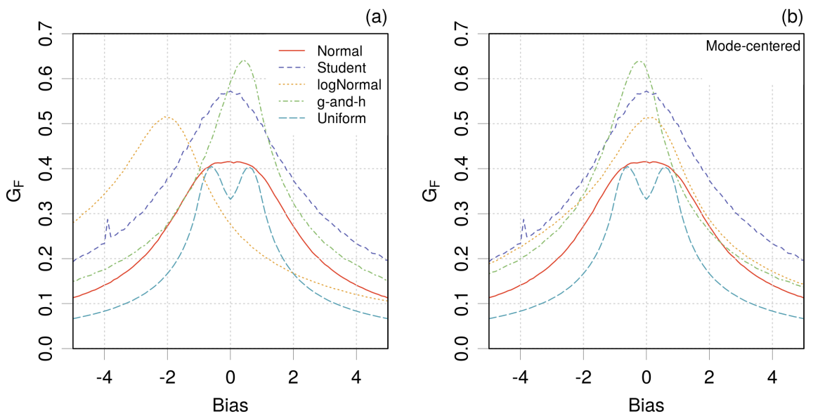
The zero-centered unimodal symmetric distributions (normal and Student’s-) have their maximal value when the bias is null. The curve for the uniform distribution reaches when the distribution is centered or shifted by . For intermediate absolute values of the bias, the folded distribution is not uniform and presents higher values of . The value decreases when the bias is large enough to exclude zero from the range of non-null densities. Having heavier tails, the Student’s- distribution has a larger Gini coefficient than the normal. Any added bias leads to a decrease of .
The decay curves are symmetric with respect to the sign of the bias. This is no longer the case for asymmetric distributions (lognormal and -and-), for which the peak is reached for non-null values of the bias and the decay curves are non-symmetric.
In Fig. 2(b) we plotted similar curves for distributions centered on their mode before adding a bias (the symmetric distributions have been left unchanged). This shows that the maximal value of is reached when the mode of the distribution is at, or near, the origin. This assertion is validated in the next section (Sect. 4.2).
Another important point illustrated by these curves is that the level of information that can be recovered from is not uniform over the range of values. For instance, might as well occur for a centered normal distribution as for positively or negatively biased Student’s-, lognormal of -and- distributions, whereas values above 0.41 exclude normal and uniform distributions. Within the restrictions on the distributions shapes we considered above, one might infer that a value smaller than is likely to reveal a biased error distribution, while a value above is likely to signal distributions with one or two extended tail(s) (compared to normal tails), and with a possible bias. Between these bounds lies a blind zone where compensation between bias and shape factors prevent any inference on either of them.
4.2 Does mode-centering maximize ?
In order to avoid the blind zone effect observed above and be able to characterize the shape of a distribution from its value, mode-centering seems to offer an interesting way to relieve the bias/shape compensation. Mode-centering a distribution results in a folded distribution where both tails overlap and mix, but it ensures that the contribution of the most-extended tail will prevail. In absence of mode-centering, when a biased distribution has a large tail encompassing zero, the folding around zero might considerably reduce this tail.
The assertion that mode-centering maximizes is tested here by comparing the results for mode-centering with those obtained by explicitly maximizing the Gini coefficient with respect to a bias value. We define as the value of the bias which maximizes
| (15) |
and note . This equation is solved numerically by the Nelder and Mead optimizer [39].
The values of and were computed for the literature datasets and compared to the mode and respectively, through -scores
| (16) |
and
| (17) |
where the uncertainties are estimated by bootstrap.
In the hypothesis of a normal distribution of -scores, a test threshold of 2 is generally chosen for the absolute value of the -score [40]. For absolute values above 2, there is less than 5 percent of probability that the difference is due to sampling effects. For values below, one does not reject the hypothesis that the compared values are equal [3].
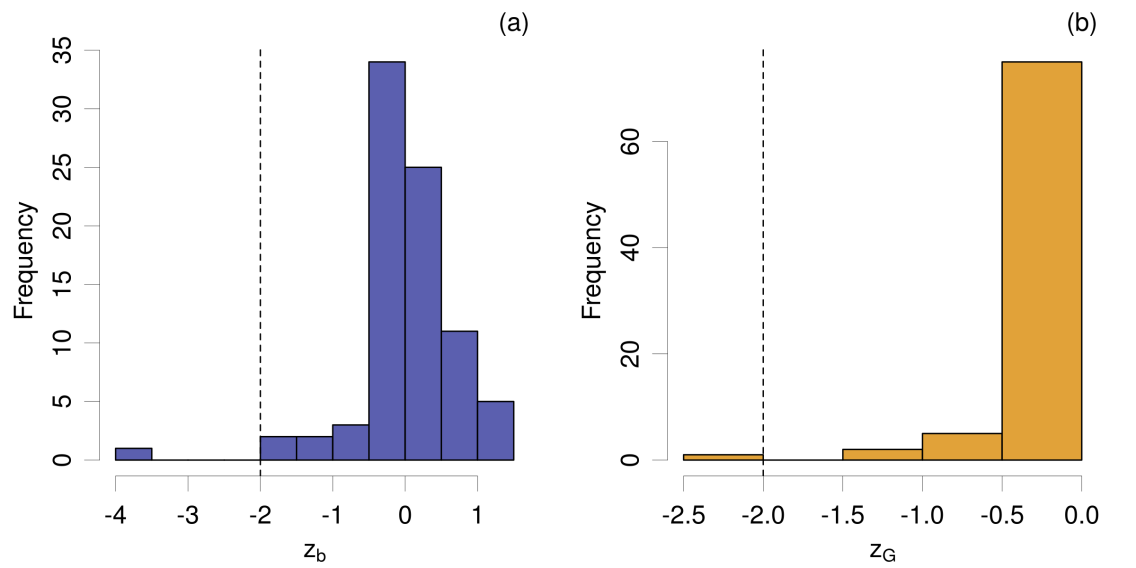
Histograms for the -scores are shown in Fig. 3. At the exception of one point, the absolute value of all -score values are smaller than 2, and we have therefore no reason to reject the hypothesis that these values are equal considering their uncertainty. The outlying point, with and corresponds to the MP2 method in dataset ZAS2019, which has a practically normal distribution [5]. One has and for a distance of 1.07 between the mode and , to be compared to the standard deviation of the distribution, 1.7. As seen in Fig. 2(a), there is a flat area near the top of the curve as a function of bias for a normal distribution: very small deviations from a perfect normal distribution (as hinted to by the value of being larger than 0.41) can deviate the optimal point over a wide range.
For all practical purposes in the present study, one can therefore estimate that mode-centering maximizes the value of the Gini coefficient, at a fraction of the computing cost for the search for . We further note that for distributions having distinct mean and mode, centering on the mean would not maximize and therefore preserve some of the ambiguity due to bias/shape compensation.
4.3 versus
We note the Gini coefficient of mode-centered folded distributions . Fig. 4(a) displays versus for the literature datasets. It is clear that mode-centering increases all values, i.e. for all datasets, within the estimation uncertainties. The -scale is now reduced to values above 0.4, in conformity with our interpretation that all values below were due to bias.
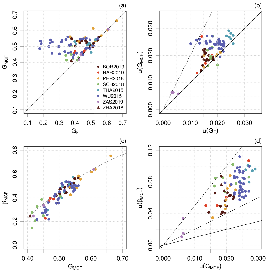
The uncertainties are reported in Fig. 4(b), showing that for some datasets the uncertainty on is larger than the uncertainty on , up to a factor two. This extra uncertainty is due to the uncertainty on the mode value. We note also a size effect, the smallest datasets (THA2015, ) having the largest uncertainty, and the largest dataset (ZAS2019, , the smallest one.
4.4 as a shape statistic
In parallel with the Gini coefficient, the skewness of the distribution has also been considered as an estimator of inequality [11]. One is interested here in comparing with , which is the skewness (Eq. 9) of the mode-centered folded distribution.
The values for our selection of literature datasets is shown in Fig. 4(c). There is an excellent correlation between those statistics, considering the uncertainties reported in Fig. 4(d). Using model datasets of large size () for Student’s- and -and- distributions with a range of shape parameters, one observes a nearly perfect non-linear correlation (dashed line, resulting from a quadratic fit of the sampled values). The dispersion of the points for the literature datasets about this curve is mostly due to statistical uncertainty (the points for the largest dataset (ZAS2019, ) are very close to the curve). It is important to note that the uncertainty on is a factor two to five smaller than the uncertainty on , and therefore performs better for smaller datasets.
We can therefore conclude that is apt at estimating the heaviness of the errors distribution tail after mode-centering and folding. In order to appreciate the information about the signed error distribution that can be extracted from , we plotted it against the skewness and excess kurtosis (Fig. 5).
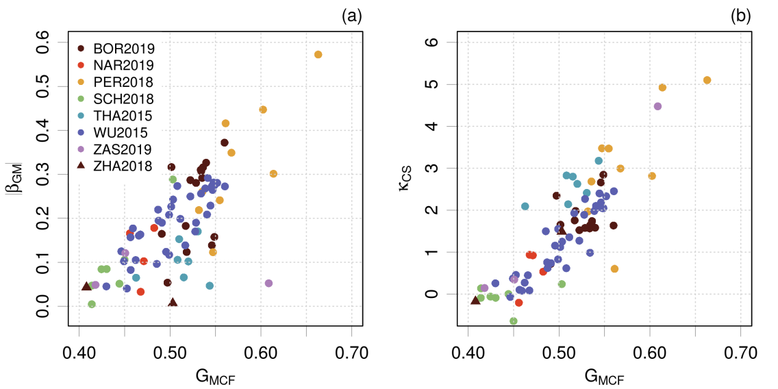
Considering skewness (Fig. 5(a)), all the points seem to lie within an angular sector, indicating that distributions with large skewness have necessarily large values. For instance, if the absolute value of the skewness is above 0.3, is larger than 0.5. Reciprocally, provides only an upper limit to (for , the absolute value of the skewness cannot be above 0.4). For kurtosis (Fig. 5(b)), there is a lax positive trend between both statistics, and, globally, large values of are associated with large excess kurtosis, which might be due to heavy tails or outliers. In both graphs, values of below 0.45 are associated with low skewness and excess kurtosis. Although information is lost because of folding, can still provide some information about the shape of the distribution of signed errors, and notably about the kurtosis.
Let us consider a few examples to illustrate this point. We see in Fig. 5 that most points fall between 0.4 and 0.55, but a few methods reach higher values. The largest value in this study is 0.66 (orange dot) for method CAM-B3LYP in the PER2018 set [2] (cf. Table 2). This corresponds to large values of both and . The authors discussed how this DFA is in the head group of two methods with similar MUE values, but does not minimize the risk of large errors (Sect. II.A [2]). From the same set, B3LYP has the second largest value (0.61) and presents the same tail features than CAM-B3LYP. The third largest value (0.61, violet dot) belongs to the ZAS2019 dataset, and it presents a null skewness and a large kurtosis. An in-depth study has been published for this case [5], where the errors distribution for the SLATM-L2 method was shown to have large tails, despite having the smallest MUE among the compared methods. In the same set, the MP2 method has a practically normal errors distribution and can be found in the lower part of the Gini scale (0.42). This analysis can be repeated for the ten methods with largest values (Table 2), showing that large values point indeed towards error sets with high kurtosis and/or skewness.
| Dataset | Methods | ||||||
|---|---|---|---|---|---|---|---|
| PER2018 | CAM-B3LYP | 0. | 663(16) | 0. | 572(57) | 5. | 1(1.3) |
| PER2018 | B3LYP | 0. | 614(20) | 0. | 301(74) | 4. | 93(96) |
| ZAS2019 | SLATM_L2 | 0. | 6086(59) | 0. | 052(22) | 4. | 48(25) |
| PER2018 | LC-PBE | 0. | 602(20) | 0. | 447(64) | 2. | 82(82) |
| PER2018 | PBE0 | 0. | 568(24) | 0. | 349(63) | 2. | 99(86) |
| PER2018 | BH&HLYP | 0. | 561(20) | 0. | 416(52) | 0. | 60(48) |
| WU2015 | HCTHhyb | 0. | 560(24) | -0. | 273(84) | 2. | 45(83) |
| BOR2019 | HLE16 + SOC | 0. | 560(19) | 0. | 372(43) | 1. | 64(47) |
| PER2018 | BLYP | 0. | 555(20) | -0. | 241(67) | 3. | 47(78) |
| WU2015 | B97-2 | 0. | 552(22) | -0. | 281(80) | 2. | 33(77) |
4.5 Application of to ranking
To evaluate the interest of in a practical scenario, one might consider it as an alert mechanism to complement a MUE ranking. But a question remains: “What is the threshold for one should use to detect problematic error distributions ?” We have seen above that the ten largest values, above 0.55, point to distributions with notable tails. We propose for the present study to adopt an alert value based on the median of the values for our full dataset (0.51) and round it to 0.5. This might be reevaluated when more data are analyzed. Using this threshold, one might flag distributions suspected of having tails unsuitable for reliable predictions.
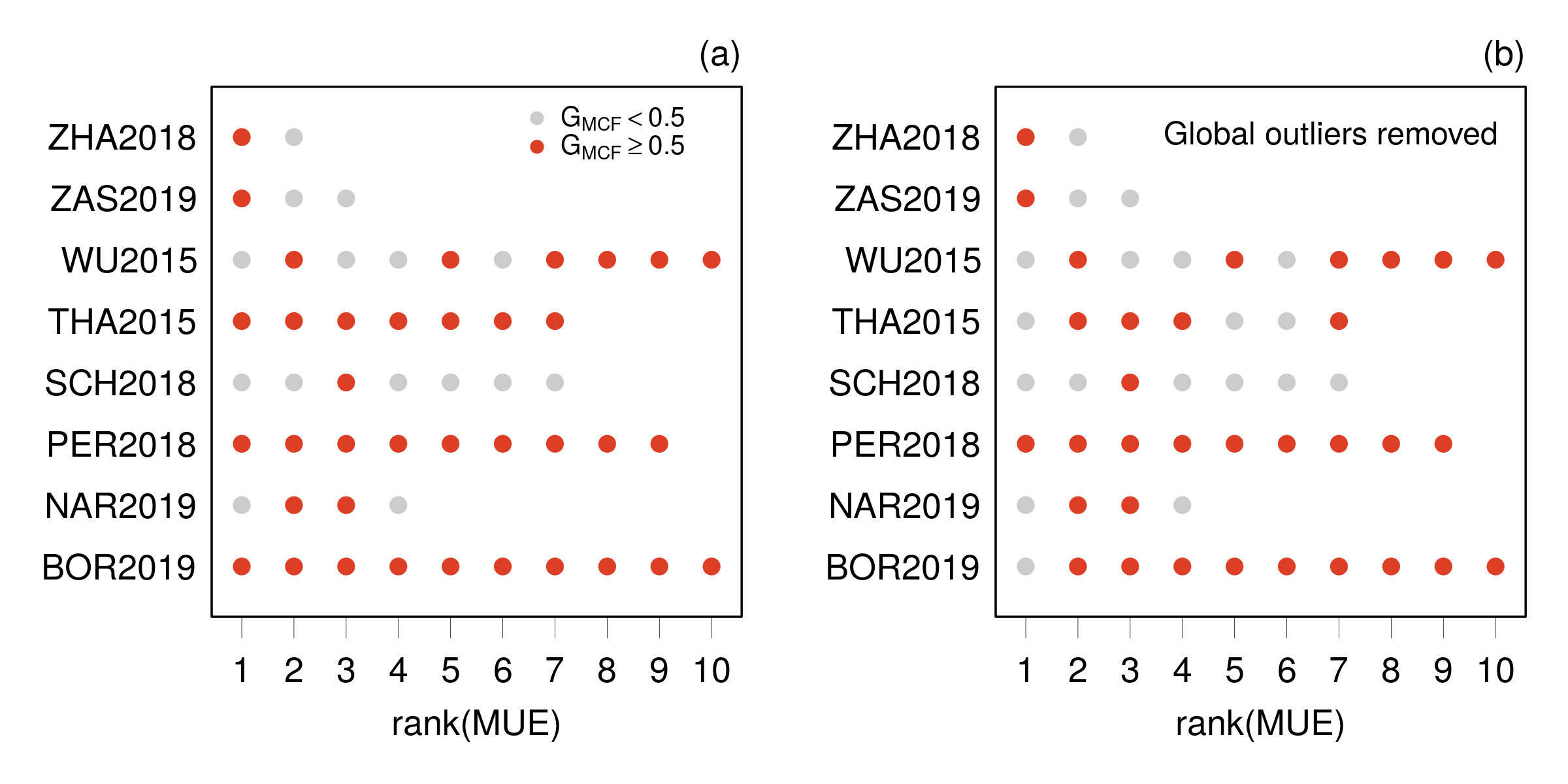
Fig. 6(a) shows, for each dataset, the flagging of the methods with best ranking. If one considers the first rank, five methods are flagged, but it is striking that three datasets have all their 10 lowest MUE-ranked methods flagged (BOR2019, PER2018 and THA2015). For BOR2019, all methods present some excess kurtosis and variable levels of skewness. We can relate this to an increasing trend of the errors with the bandgap value [4]. In the case of PER2018, the error distributions present also large skewness and kurtosis, that can be associated with the chemical heterogeneity of the dataset [2]. For THA2015, it was noted previously [35, 4] that some experimental reference data with large measurement uncertainty could not be reproduced by any method in the studied set. These outliers contribute to the tails of all the error distributions (so-called global outliers) and affect values. Note that, more generally, reference data are not necessarily the origin of global outliers, as a missing physical contribution in the tested methods could produce similar effects.
To explore the role of global outliers, Fig. 6(b) reports the same analysis after search and removal of global outliers, defined as systems lying out of the interval for all methods of a dataset. The removal of 6 systems affects strongly the case THA2015, confirming the previous analysis. The results for BOR2019 are mostly unchanged, except for the best MUE-ranked method (mBJ) which benefits from the removal of a single global outlier. No effect is observed for the PER2018 dataset, confirming the intrinsic heavy-tailed shape of these heterogeneous atomization energy error sets [2].
The other datasets with leading -flagged methods are ZAS2019 and ZHA2018. The former has already been discussed (Sect. 4.4), and the removal of several global outliers has no impact. In the case ZHA2018, the first MUE-ranked method is SCAN, which has a value just above the threshold (0.503), presents no skewness and a slight level of kurtosis. Removal of 4 global outliers does not improve the shape of the errors distribution. However, the errors on the formation enthalpies present a linear trend as a function of the calculated values. Correcting this trend [1] improves slightly the performance and the shape of the SCAN distribution, but most notably of the PBE distribution, which performances get indistinguishable from those of SCAN (Table 3).
| Methods | MUE | MSE | ||||||||||
|---|---|---|---|---|---|---|---|---|---|---|---|---|
| (kcal/mol) | (kcal/mol) | (kcal/mol) | ||||||||||
| PBE | 0. | 2106(98) | -0. | 205(10) | 0. | 467(34) | -0. | 043(64) | -0. | 17(28) | 0. | 408(18) |
| SCAN | 0. | 1024(69) | -0. | 0165(97) | 0. | 291(21) | -0. | 007(67) | 1. | 49(53) | 0. | 503(19) |
| lc-PBE | 0. | 0923(61) | 0. | 0 | 0. | 287(38) | -0. | 138(71) | 1. | 02(43) | 0. | 479(24) |
| lc-SCAN | 0. | 0917(63) | 0. | 0 | 0. | 276(26) | -0. | 082(67) | 1. | 27(41) | 0. | 475(20) |
4.6 Limits of the coefficient
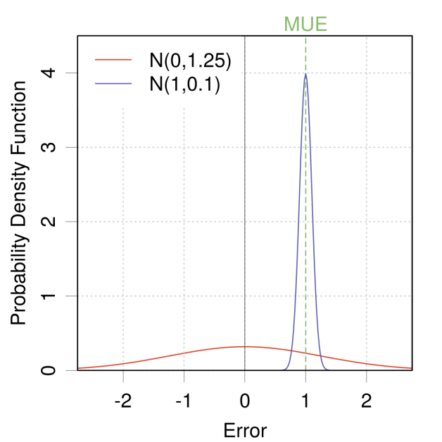
We have shown above that might be a useful complement to the usual ranking statistics, in order to detect error distributions with shapes that might reveal problem in prediction reliability. However there remains cases where the index is insufficient to reveal underlying problems. Fig. 7 proposes a scenario of two normal distributions () with the same value of the MUE (1.0), and yet very different risks of large prediction errors. This is clearly a case showing that a quantile-based statistic, such as , is an essential complement to the MUE.
5 Conclusion
The Gini coefficient presents an interesting addition to the computational chemistry benchmarking statistical toolbox. We focused here on its properties in relation with features of the error distributions, such as bias and shape (skewness and kurtosis). The interest of the Gini coefficient is that it correlates with these features, and offers a one-number summary. This is also one of its weaknesses, as there is no unique mapping from the Gini coefficient to these features.
To unscramble this situation, we propose to use the Gini coefficient of the mode-centered distributions, , which offers a simpler to interpret, shape-based, measure of tailedness. Large values, e.g. above 0.5, alert us about large tails that might be due to large skewness, kurtosis and/or the presence of outliers. For high ranking methods, this is an incentive to inspect closely the error distributions and check if the selected methods might have problems of reliability in their predictions. It might then be worth to investigate if the distorted shape of the distribution is due to systematic trends in the errors, as they can often be corrected by simple linear transformations [41, 1, 42, 43, 44]. The impact of such corrections on the shape of error distributions is the prospect of further studies.
Supplementary Information
Statistics, ECDFs and Lorenz curves for the literature datasets are openly available at the following URL: https://doi.org/10.5281/zenodo.4333217
Data availability statement
The data and codes that support the findings of this study are openly available at the following URL: https://doi.org/10.5281/zenodo.4333217
Dedication
This work is dedicated to Ramon Carbó-Dorca for his 80th birthday. It reflects his interest for cross-disciplinary aspects of science, especially the role of mathematics in chemistry.
References
- [1] P. Pernot, B. Civalleri, D. Presti, and A. Savin. Prediction uncertainty of density functional approximations for properties of crystals with cubic symmetry. J. Phys. Chem. A, 119:5288–5304, 2015. doi:10.1021/jp509980w.
- [2] P. Pernot and A. Savin. Probabilistic performance estimators for computational chemistry methods: the empirical cumulative distribution function of absolute errors. J. Chem. Phys., 148:241707, 2018. doi:10.1063/1.5016248.
- [3] P. Pernot and A. Savin. Probabilistic performance estimators for computational chemistry methods: Systematic improvement probability and ranking probability matrix. I. Theory. J. Chem. Phys., 152:164108, 2020. doi:10.1063/5.0006202.
- [4] P. Pernot and A. Savin. Probabilistic performance estimators for computational chemistry methods: Systematic improvement probability and ranking probability matrix. II. Applications. J. Chem. Phys., 152:164109, 2020. doi:10.1063/5.0006204.
- [5] P. Pernot, B. Huang, and A. Savin. Impact of non-normal error distributions on the benchmarking and ranking of Quantum Machine Learning models. Mach. Learn.: Sci. Technol., 1:035011, 2020. doi:10.1088/2632-2153/aba184.
- [6] M. Bonato. Robust estimation of skewness and kurtosis in distributions with infinite higher moments. Finance Research Letters, 8:77–87, 2011. doi:10.1016/j.frl.2010.12.001.
- [7] M. O. Lorenz. Methods of measuring the concentration of wealth. Publications of the American Statistical Association, 9:209–219, 1905. doi:10.1080/15225437.1905.10503443.
- [8] C. Gini. Variabilità e mutabilità. 1912.
- [9] C. Damgaard and J. Weiner. Describing inequality in plant size or fecundity. Ecology, 81:1139–1142, 2000. doi:10.2307/177185.
- [10] I. I. Eliazar and I. M. Sokolov. Measuring statistical heterogeneity: The Pietra index. Physica A, 389:117–125, 2010. doi:10.1016/j.physa.2009.08.006.
- [11] R. B. Bendel, S. S. Higgins, J. E. Teberg, and D. A. Pyke. Comparison of skewness coefficient, coefficient of variation, and Gini coefficient as inequality measures within populations. Oecologia, 78:394–400, 1989. doi:10.1007/BF00379115.
- [12] M. K. Florian, N. Li, and M. D. Gladders. The Gini coefficient as a morphological measurement of strongly lensed galaxies in the image plane. Astrophys. J., 832:168, 2016. doi:10.3847/0004-637X/832/2/168.
- [13] N. Hurley and S. Rickard. Comparing measures of sparsity. IEEE Transactions on Information Theory, 55:4723–4741, 2009. doi:10.1109/TIT.2009.2027527.
- [14] C. Kleiber. The Lorenz curve in economics and econometrics. techreport, TU Dortmund, March 2005. doi:10.17877/DE290R-14481.
- [15] P. M. Dixon, J. Weiner, T. Mitchell-Olds, and R. Woodley. Bootstrapping the Gini coefficient of inequality. Ecology, 68:1548–1551, 1987. doi:10.2307/1939238.
- [16] D. Ruppert. What is kurtosis?: An influence function approach. The American Statistician, 41:1, 1987. doi:10.2307/2684309.
- [17] R. A. Groeneveld and G. Meeden. Measuring skewness and kurtosis. The Statistician, 33:391–399, 1984. URL: http://www.jstor.org/stable/2987742, doi:10.2307/2987742.
- [18] K. Suaray. On the asymptotic distribution of an alternative measure of kurtosis. Int. J. Adv. Stat. Proba., 3:161–168, 2015. doi:10.14419/ijasp.v3i2.5007.
- [19] E. L. Crow and M. M. Siddiqui. Robust estimation of location. Journal of the American Statistical Association, 62:353–389, 1967. doi:10.2307/2283968.
- [20] D. R. Bickel. Robust estimators of the mode and skewness of continuous data. Comput. Stat. Data Anal., 39:153–163, 2002. doi:10.1016/S0167-9473(01)00057-3.
- [21] S. B. Hedges and P. Shah. Comparison of mode estimation methods and application in molecular clock analysis. BMC Bioinformatics, 4:31, 2003. doi:10.1186/1471-2105-4-31.
- [22] G. J. Glasser. Variance formulas for the mean difference and coefficient of concentration. J. Am. Stat. Assoc., 57:648–654, 1962. doi:10.1080/01621459.1962.10500553.
- [23] A. Zeileis. ineq: Measuring Inequality, Concentration, and Poverty, 2014. R package version 0.2-13. URL: https://CRAN.R-project.org/package=ineq.
- [24] F. E. Harrell and C. Davis. A new distribution-free quantile estimator. Biometrika, 69:635–640, 1982. doi:10.2307/2335999.
- [25] R. R. Wilcox and D. M. Erceg-Hurn. Comparing two dependent groups via quantiles. J. App. Stat., 39:2655–2664, 2012. doi:10.1080/02664763.2012.724665.
- [26] B. Efron. Bootstrap Methods: Another Look at the Jackknife. Ann. Stat., 7(1):1–26, January 1979. doi:10.1214/aos/1176344552.
- [27] R Core Team. R: A Language and Environment for Statistical Computing. R Foundation for Statistical Computing, Vienna, Austria, 2019. URL: http://www.R-project.org/.
- [28] R. Gentleman, V. Carey, W. Huber, and F. Hahne. genefilter: methods for filtering genes from high-throughput experiments, 2019. R package version 1.68.0. doi:10.18129/B9.bioc.genefilter.
- [29] A. Canty and B. D. Ripley. boot: Bootstrap R (S-Plus) Functions, 2019. R package version 1.3-22.
- [30] M. Evans, N. Hastings, and B. Peacock. Statistical Distributions. Wiley-Interscience, 3rd edition, 2000.
- [31] D. C. Hoaglin. Exploring data tables, trends, and shapes, chapter Summarizing shape numerically: The g-and-h distributions, pages 461–513. Wiley, New York, 1985.
- [32] P. Borlido, T. Aull, A. W. Huran, F. Tran, M. A. Marques, and S. Botti. Large-scale benchmark of exchange–correlation functionals for the determination of electronic band gaps of solids. J. Chem. Theory Comput., 15:5069–5079, 2019. doi:10.1021/acs.jctc.9b00322.
- [33] B. Narayanan, P. C. Redfern, R. S. Assary, and L. A. Curtiss. Accurate quantum chemical energies for 133000 organic molecules. Chem. Sci., 10:7449–7455, 2019. doi:10.1039/c9sc02834j.
- [34] P. S. Schmidt and K. S. Thygesen. Benchmark database of transition metal surface and adsorption energies from many-body perturbation theory. J. Phys. Chem. C, 122:4381–4390, 2018. doi:10.1021/acs.jpcc.7b12258.
- [35] A. J. Thakkar and T. Wu. How well do static electronic dipole polarizabilities from gas-phase experiments compare with density functional and MP2 computations? J. Chem. Phys., 143:144302, 2015. doi:10.1063/1.4932594.
- [36] T. Wu, Y. N. Kalugina, and A. J. Thakkar. Choosing a density functional for static molecular polarizabilities. Chem. Phys. Lett., 635:257–261, 2015. doi:10.1016/j.cplett.2015.07.003.
- [37] P. Zaspel, B. Huang, H. Harbrecht, and O. A. von Lilienfeld. Boosting quantum machine learning models with a multilevel combination technique: Pople diagrams revisited. J. Chem. Theory Comput., 15(3):1546–1559, 2019. doi:10.1021/acs.jctc.8b00832.
- [38] Y. Zhang, D. A. Kitchaev, J. Yang, T. Chen, S. T. Dacek, R. A. Sarmiento-Perez, M. A. L. Marques, H. Peng, G. Ceder, J. P. Perdew, and J. Sun. Efficient first-principles prediction of solid stability: Towards chemical accuracy. npj Comput. Mater., 4:9, 2018. doi:10.1038/s41524-018-0065-z.
- [39] J. A. Nelder and R. Mead. A Simplex Method for Function Minimization. The Computer Journal, 7:308–313, 1965. doi:10.1093/comjnl/7.4.308.
- [40] R. N. Kacker, R. Kessel, and K.-D. Sommer. Assessing differences between results determined according to the guide to the expression of uncertainty in measurement. J. Res. Nat. Inst. Stand. Technol., 115(6):453, 2010. doi:10.6028/jres.115.031.
- [41] K. Lejaeghere, J. Jaeken, V. V. Speybroeck, and S. Cottenier. Ab initio based thermal property predictions at a low cost: An error analysis. Phys. Rev. B, 89:014304, jan 2014. doi:10.1103/physrevb.89.014304.
- [42] K. Lejaeghere, L. Vanduyfhuys, T. Verstraelen, V. V. Speybroeck, and S. Cottenier. Is the error on first-principles volume predictions absolute or relative? Comput. Mater. Sci., 117:390–396, 2016. doi:10.1016/j.commatsci.2016.01.039.
- [43] J. Proppe, T. Husch, G. N. Simm, and M. Reiher. Uncertainty quantification for quantum chemical models of complex reaction networks. Faraday Discuss., 195:497–520, 2016. doi:10.1039/c6fd00144k.
- [44] J. Proppe and M. Reiher. Reliable estimation of prediction uncertainty for physicochemical property models. J. Chem. Theory Comput., 13:3297–3317, 2017. doi:10.1021/acs.jctc.7b00235.