Soft-drop grooming for hadronic event shapes

Abstract

Soft-drop grooming of hadron-collision final states has the potential to significantly reduce the impact of non-perturbative corrections, and in particular the underlying-event contribution. This eventually will enable a more direct comparison of accurate perturbative predictions with experimental measurements. In this study we consider soft-drop groomed dijet event shapes. We derive general results needed to perform the resummation of suitable event-shape variables to next-to-leading logarithmic (NLL) accuracy matched to exact next-to-leading order (NLO) QCD matrix elements. We compile predictions for the transverse-thrust shape accurate to $\text{NLO}+\text{NLL}^{\prime}$ using the implementation of the CAESAR formalism in the SHERPA event generator framework. We complement this by state-of-the-art parton- and hadron-level predictions based on NLO QCD matrix elements matched with parton showers. We explore the potential to mitigate non-perturbative corrections for particle-level and track-based measurements of transverse thrust by considering a wide range of soft-drop parameters. We find that soft-drop grooming indeed is very efficient in removing the underlying event. This motivates future experimental measurements to be compared to precise QCD predictions and employed to constrain non-perturbative models in Monte-Carlo simulations.

1 Introduction

Event-shape variables attribute simple real numbers to a scattering event, determined by the momenta of the final-state particles, that characterise geometric properties of the event. Their distributions offer a wide range of potential applications in collider phenomenology. This includes precision QCD studies, e.g. extractions of the strong coupling, the discrimination of hypothetical new physics from Standard Model expectations, as well as stress-tests, validation and tuning of Monte Carlo event generators. Aside from event generators, theoretical predictions for event shapes can be obtained from fixed-order and resummation calculations. However, in general, event-shape observables are rather susceptible to non-perturbative corrections, i.e. hadronisation effects and the underlying event. These need to be taken into account when comparing high-precision calculations with experimental data, e.g. through the evaluation of power corrections Dokshitzer:1995zt ; Dokshitzer:1995qm ; Dokshitzer:1997ew , or, via phenomenological models, as done in event generators Buckley:2011ms . Their sensitivity to non-perturbative phenomena makes event-shape observables very valuable for the tuning of Monte Carlo generators.

There exists a vast amount of event-shape studies for $e^{+}e^{-}$ colliders Heister:2003aj ; Abbiendi:2004qz ; Abdallah:2003xz ; Achard:2004sv for DIS Aktas:2005tz ; Chekanov:2006hv , and corresponding higher-order and higher-logarithmic perturbative QCD predictions, see for instance Abbate:2010xh ; Abbate:2012jh ; Hoang:2014wka ; Banfi:2014sua ; Tulipant:2017ybb ; Bell:2018gce ; Kang:2013lga ; Becher:2015gsa ; Becher:2015lmy ; Dixon:2018qgp ; Gao:2019ojf ; Dixon:2019uzg ; Gehrmann:2019hwf . Event shapes such as thrust can be consistently defined also for hadron colliders Banfi:2004nk , but despite their great potential, they have received comparably little attention from experiments at hadron colliders to date.

Resummed predictions for event shapes, e.g. at next-to-leading logarithmic (NLL) accuracy, can be derived and matched to next-to-leading order (NLO) calculations. Ref. Banfi:2010xy presented an extensive phenomenological study of a variety of event shapes in dijet production under Tevatron and LHC conditions, based on $\text{NLO}+\text{NLL}^{\prime}$ predictions as well as Monte Carlo simulations. The smaller number of experimental studies of event-shape observables in hadronic collisions is certainly related to their pronounced sensitivity to non-perturbative corrections Banfi:2010xy , which complicates the interpretation of measurements in terms of perturbative predictions. Additional complications arise from constraints on the measurement acceptance region, e.g. a maximum rapidity range, $|y|\leq y_{\text{max}}$, or, a non-vanishing particle (track) transverse momentum cut, $p^{\text{track}}_{T,\text{min}}$, that hinder the direct comparison between idealised theoretical predictions and experiment. Some recent LHC measurements of event-shape variables have been based on reconstructed jets, rather than particles, as input for the observable calculation Aad:2012np ; Khachatryan:2014ika ; Sirunyan:2018adt ; Aad:2020fch . While this eases the evaluation of systematic uncertainties and acceptance corrections, it makes it extremely difficult to address them beyond a fixed-order calculation or Monte Carlo simulations.

With this work we follow the original approach of using particles as inputs to the observable. However, we consider grooming the event using Soft Drop Larkoski:2014wba , and only use the surviving constituent particles as inputs to the event-shape calculation. This provides the potential to significantly reduce the impact of non-perturbative effects while retaining the ability to analytically address these observables. As a concrete example we focus on the transverse-thrust shape. Through variations of the grooming parameters its underlying-event sensitivity can be regulated, providing additional means to tune the corresponding phenomenological models. Furthermore, the impact of using a finite maximum input-particle rapidity and minimum transverse momentum can be diminished by grooming. In fact, for sufficiently hard grooming a rather direct correspondence between perturbative predictions and hadron-level results is found. In Refs. Baron:2018nfz ; Marzani:2019evv similar observations have been made for soft-drop thrust in $e^{+}e^{-}$ collisions, where a reduced sensitivity to hadronisation effects was observed. Many other jet-substructure techniques for underlying-event mitigation exist, for example Butterworth:2008iy ; Ellis:2009su ; Krohn:2009th ; Dasgupta:2013ihk ; Dreyer:2018tjj with a detailed overview given in Marzani:2019hun . However, these approaches are restricted to grooming the constituents of a given jet only. Soft-drop grooming individual jets at hadron colliders is also intensely studied theoretically, see e.g. Frye:2016aiz ; Marzani:2017kqd ; Kang:2018jwa ; Kang:2018vgn ; Bell:2018vaa ; Kang:2019prh ; Hoang:2019ceu ; Kardos:2020ppl ; Kardos:2020gty ; Anderle:2020mxj for recent results. With this work we suggest to extend those methods to grooming of the entire event, thereby generalising the work in Baron:2018nfz ; Marzani:2019evv to global event shapes at hadron colliders.

We derive resummed predictions at $\text{NLO}+\text{NLL}^{\prime}$ accuracy for soft-drop transverse thrust by employing the implementation of the CAESAR resummation formalism Banfi:2004yd in the SHERPA event generator framework Gerwick:2014gya ; Gleisberg:2008ta ; Bothmann:2019yzt . We compare the results against parton-level shower Monte Carlo predictions before focusing on the mitigation of underlying-event effects through soft-drop grooming.

This paper is organised as follows: in Sec. 2 we give a prescription to apply soft-drop to global event shape observables for dijet events in hadronic collisions. The $\text{NLO}+\text{NLL}^{\prime}$ resummation and matching calculation are discussed in Sec. 3. In Sec. 4 we present predictions for soft-drop thrust in dijet-event final states at the LHC. We then compare resummed results and parton-shower simulations, and study the sensitivity to non-perturbative corrections as well as experimentally motivated acceptance cuts. Our conclusions are presented in Sec. 5.

2 Soft drop for hadronic event shapes

With all final-state particles contributing to the observable calculation, event-shape variables can be particularly sensitive to non-perturbative corrections. This we illustrate here for the transverse-thrust observable, which we will use throughout the paper as concrete example. This hadron-collider variant of thrust is defined as

$$\tau_{\perp}\equiv 1-\max_{\vec{n}_{\perp}}\left(\frac{\sum_{i}|\vec{p}_{T,i}\cdot\vec{n}_{\perp}|}{p_{T,\text{tot}}}\right)\;,\quad p_{T,\text{tot}}=\sum\limits_{i}p_{T,i}\,,$$ (1)

with the sum extending over all final-state particles, and $\vec{p}_{T,i}$ the respective two-component transverse-momentum vector with length $p_{T,i}=|\vec{p}_{T,i}|$. The unit vector $\vec{n}_{\perp}$ that maximises the sum in Eq. (1) defines the transverse-thrust axis. As a three-jet observable, transverse thrust quantifies the deviation from the back-to-back event configuration.

In Fig. 1 we present results obtained with the SHERPA generator at different stages of the event evolution, i.e. after parton showering but without underlying event (PL), with the underlying-event contribution included (PL+UE), and fully hadronised (HL+UE). We consider dijet-production at $\sqrt{s}=13\;\text{TeV}$ with the leading-jet transverse momentum above $200\;\text{GeV}$ and $500\;\text{GeV}$, respectively. Further details on the event selections and generator settings can be found in Secs. 2.2 and 4.1. We can observe that the inclusion of the underlying event significantly shifts the distribution, corresponding to up to 40% corrections in the peak region for events with a jet above $200\;\text{GeV}$. Even for the higher transverse-momentum criterion ($500\;\text{GeV}$) the underlying event still retains a similar impact. Hadronisation corrections are comparably smaller. Qualitatively hadronisation pushes events to somewhat higher values of transverse thrust, resulting in corrections of order 10% in the peak region and even more sizeable in the low-$\tau_{\perp}$ tail, i.e. $\ln(\tau_{\perp})\lesssim-3$. This strong susceptibility of the observable to non-perturbative effects over its whole range makes the comparison of experimental measurements with purely perturbative calculations rather indirect and plagued by significant modelling uncertainties.

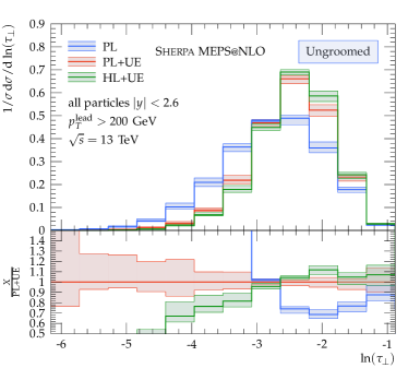
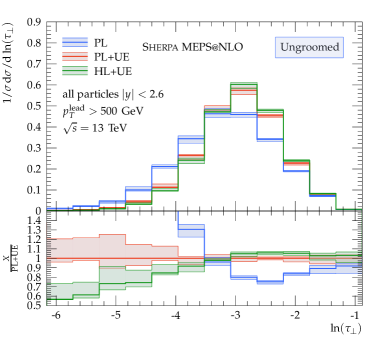
Figure 1: The transverse-thrust distributions for events with a leading-jet transverse momentum $p^{\text{lead}}_{T}>200\;\text{GeV}$ (left) and $p^{\text{lead}}_{T}>500\;\text{GeV}$ (right). Further details on the event-selection cuts are given in Sec. 2.2. Shown are MEPS@NLO predictions obtained with SHERPA at parton level (PL), with the underlying event included (PL+UE), and at full hadron level (HL+UE). The lower panels show the ratios with respect to the PL+UE prediction.

Transverse thrust has been measured by the Tevatron Aaltonen:2011et and LHC experiments Aad:2012np ; Khachatryan:2014ika ; Sirunyan:2018adt ; Aad:2020fch . However, recent measurements are based on reconstructed jets as inputs to the observable calculation, which simplifies dealing with the large underlying event contributions but prevents a direct comparison to perturbative predictions, see for example the discussion in Banfi:2010xy . Those have so far been presented at NLO QCD Nagy:2003tz and resummed to $\text{NLO}+\text{NLL}^{\prime}$ level in the CAESAR framework Banfi:2003je , and more recently the resummation has been extended to NNLL accuracy in the context of soft-collinear effective field theory Becher:2015gsa ; Becher:2015lmy . In this work we consider full particle-level final states, i.e. charged tracks, as input to the observable calculation. To mitigate the impact of non-perturbative effects, in particular the underlying event, we suggest soft-drop grooming the event prior to the observable evaluation. We argue that the developed method should be applicable to the standard set of observables studied by the experiments, and the derived formulae are given for a general observable within the limitations of the CAESAR approach to resummation. For concreteness, we focus on transverse thrust, as the "standard candle" event-shape variable, in our phenomenological studies.

2.1 Definition groomed event shapes

Soft drop has a wide range of applications, including being used in boosted-particle tagging or for pile-up mitigation. The method introduced in Larkoski:2014wba has originally been designed as a jet-substructure technique to remove soft wide-angle radiation from a jet. For a jet of radius $R_{\text{SD}}$ the constituents get reclustered using the Cambridge–Aachen (C/A) algorithm Dokshitzer:1997in ; Wobisch:1998wt . Then the last C/A clustering step is undone and the resulting two subjets are subjected to the soft-drop criterion

$$\frac{\min(p_{T,i},p_{T,j})}{p_{T,i}+p_{T,j}}\geq z_{\text{cut}}\left(\frac{\Delta R_{ij}}{R_{\text{SD}}}\right)^{\beta}\,,$$ (2)

with $p_{T,i}$ the transverse momenta of the two constituent subjets with respect to the beam, and $\Delta R_{ij}^{2}=(y_{i}-y_{j})^{2}+(\phi_{i}-\phi_{j})^{2}$ their separation in the rapidity-azimuth plane. If the condition is satisfied grooming ends and the jet is the combination of these two subjets, otherwise the subjet with smaller transverse momentum is removed from the jet and the procedure is continued for the harder subjet. The two relevant parameters are the threshold $z_{\text{cut}}$ and the angular exponent $\beta\geq 0$. It should be noted that for $\beta=0$, which corresponds to the modified Mass-Drop Tagger (mMDT) Butterworth:2008iy ; Dasgupta:2013ihk , all soft emissions at LO accuracy are groomed. This alters the logarithmic structure of the resummation leading to only single-logarithmic enhancement of the observable which is of collinear origin.

Here, we build up on work in Baron:2018nfz ; Kardos:2018kth , where soft drop has been applied to the thrust variable in $e^{+}e^{-}$ collisions Farhi:1977sg , among other event shapes. We stress that the main motivation for this is to study observables close to traditional event shapes but with reduced impact of non-perturbative effects, even though soft drop is a more general tool that could suggest alternative observable definitions by itself. Correspondingly, the event is divided into two hemispheres based on the thrust axis, and the soft-drop condition is applied to both of them. We will generalise this idea and define soft-drop groomed versions of hadronic event shapes. To this end we employ the transverse-thrust axis $\vec{n}_{\perp}$ to separate a given event into azimuthal hemispheres, $\mathcal{H}_{R}$ containing all particles with $\vec{n}_{\perp}\cdot\vec{p}_{T,i}\geq 0$, and $\mathcal{H}_{L}$ containing all particles with $\vec{n}_{\perp}\cdot\vec{p}_{T,i}<0$. For each hemisphere separately, we can then apply the standard soft-drop procedure, i.e. recluster all particles in the hemisphere into a C/A jet, then subsequently undo clustering steps and check the soft-drop criterion Eq. (2) as described above for jets. The remaining particles of both hemispheres, which we will refer to as $\mathcal{H}_{L}^{\prime}$ and $\mathcal{H}_{R}^{\prime}$, then constitute the groomed-event final state. The hemispheres do not have an auxiliary radius associated to them, so we can make a choice $R_{\text{SD}}=1$ in what follows. The result of this application of soft-drop is quite different from the usual approach of grooming jets. In general, $\beta>0$ suppresses grooming for radiation at small angles. For a jet $R_{\text{SD}}$ is typically chosen equal to the jet radius and this suppression is happening for all radiation inside the jet. However, for a hemisphere there will be cases for which $\Delta R_{ij}>R_{\text{SD}}$. For these particles, grooming will instead be even stronger. This changes the role of the parameter $\beta$, as values $\beta>0$ can result in more significant grooming. This in particular has the potential to suppress contributions from multiple-parton interactions, i.e. the underlying event, which are largely uncorrelated in angle with respect to the hard process.

We now want to calculate a given event shape with the particles that survived this grooming procedure. The exact definition of the groomed event shape for arbitrary, not necessarily soft and/or collinear configurations might however not be uniquely fixed by this prescription, and care has to be taken not to introduce issues regarding collinear safety, cf. Appendix A of Marzani:2019evv for a detailed discussion. As we are going to focus on hadronic thrust in our phenomenological studies, we give an explicit definition of its groomed variant:

$$\tau_{\perp}^{\text{SD}}\equiv\left(1-\frac{\sum_{i\in\mathcal{H}_{L}^{\prime}}|\vec{p}_{T,i}\cdot\vec{n}_{\perp,L}^{\prime}|}{\left(p_{T,\text{tot}}\right)^{\text{groomed}}}-\frac{\sum_{i\in\mathcal{H}_{R}^{\prime}}|\vec{p}_{T,i}\cdot\vec{n}_{\perp,R}^{\prime}|}{\left(p_{T,\text{tot}}\right)^{\text{groomed}}}\right)\frac{\left(p_{T,\text{tot}}\right)^{\text{groomed}}}{\left(p_{T,\text{tot}}\right)^{\text{all}}}$$ (3)

$$\text{with}\quad\vec{n}_{\perp,X}^{\prime}=\frac{\sum_{i\in\mathcal{H}_{X}^{\prime}}\vec{p}_{T,i}}{\left|\sum_{i\in\mathcal{H}_{X}^{\prime}}\vec{p}_{T,i}\right|},\quad\text{and}\quad\left(p_{T,\text{tot}}\right)^{\text{groomed}}=\sum_{i\in\mathcal{H}_{L}^{\prime}}\left|\vec{p}_{T,i}\right|+\sum_{i\in\mathcal{H}_{R}^{\prime}}\left|\vec{p}_{T,i}\right|,$$ (4)

where as indicated all sums run over the particles that survive grooming in the respective hemispheres, and $\left(p_{T,\text{tot}}\right)^{\text{all}}$ denotes the scalar sum of the transverse momenta of all particles, whether or not affected by grooming. Multiplying by the ratio of the total groomed and ungroomed transverse momentum guarantees collinear safety as mentioned above, in full analogy with the $e^{+}e^{-}$ case Baron:2018nfz ; Marzani:2019evv .

Experimental considerations

In addition to the theoretical considerations when defining an observable, it should be viable to be measured experimentally in a setup as close to the calculation as possible. The resummation and fixed-order consideration are based on the distribution of partons. After applying a correction according to some hadronisation model, or convincing ourselves that those corrections are rather small, they might be taken as a prediction for the observable as defined on all hadrons in the final state. However, those are not readily available in general in hadron-collider experiments, though for example the particle-flow method used by the CMS experiment Sirunyan:2017ulk gets rather close to the particle level. However, for our final phenomenological studies, we here define the observables based on detectable charged-particle tracks, accessible with conventional tracking techniques. Those are assumed to resemble the overall distribution of hadrons in the event, allowing us to relate to the analytic calculation. However, the use of charged tracks in practice results in several limitations.

The first experimental restriction is the rapidity range where tracks can be measured reliably. This results in a maximum rapidity $y_{\text{max}}$ within which particles are considered to contribute to the observable calculation. For transverse thrust this cut-off alters the logarithmic structure for the resummation. In Banfi:2010xy this was addressed by suggesting certain changes to the observable definitions. Here, we are going to argue that our modification, i.e. soft-drop grooming, is already sufficient. The reason for this is essentially that particles contributing to this difference in logarithmic structure will have low transverse momentum and therefore be prone to grooming. This allows us to ignore the rapidity cut-off in the resummed calculation and take it into account in the final matched distributions by including it in the fixed-order calculation.

In addition to the spatial restriction, a track-based measurement can only be performed based on charged particles with a transverse momentum above some threshold $p^{\text{track}}_{T,\text{min}}$. This conversion from all particles to charged tracks can not easily be consistently included in either resummation or fixed-order computations. However, we can make use of particle-level Monte Carlo simulations, including the parton-to-hadron transition process, to estimate the impact of this restriction. This is studied in detail along with the parton-shower results in Sec. 4. There we will also verify our assumption on the correspondence between measurements based on charged and all particles in hadronic final states.

2.2 Event selection and phase-space constraints

For completeness, we will define the full phase space we consider for both the analytic calculation and our Monte Carlo studies. We want to study dijet events in proton–proton collisions at $\sqrt{s}=13\;\text{TeV}$ centre-of-mass energy. We require events to contain at least two $R=0.4$ anti-$k_{t}$ jets Cacciari:2008gp , rather central in rapidity, and satisfying an asymmetric cut on their transverse momenta:

$$|y_{j}|<1\,,\;\;\text{and}\qquad p_{T}^{\text{lead}}\geq p_{T,\text{min}}\,,\quad p_{T}^{2\text{nd}}\geq\frac{p_{T,\text{min}}}{2}\,.$$ (5)

In what follows we consider the two choices $p_{T,\text{min}}=200\;\text{GeV}$ and $p_{T,\text{min}}=500\;\text{GeV}$. Note, these jet requirements serve as triggers only; the observable calculation is based on final-state particles, not on jets. For validation, we produce Monte Carlo samples at parton level as well as hadron level taking charged and neutral final states into account. To address the restricted acceptance for particle tracks mentioned above, only particles with $|y|\leq y_{\text{max}}=2.6$ are considered for both jet reconstruction and observable calculation. All cuts mentioned so far are implemented in the fixed-order calculations as well. For our final "experiment-level" Monte-Carlo prediction, we in addition only take into account charged particles in the hadronic final state, with a transverse momentum of

$$p^{\text{track}}_{T}\geq p^{\text{track}}_{T,\text{min}}=500\;\text{MeV}\,.$$ (6)

To study the impact of soft-drop grooming, we investigate a variety of parameter choices, i.e. $z_{\text{cut}}\in\{0.05,0.1,0.2,0.3\}$ with $\beta\in\{0,1,2\}$, while keeping $R_{\text{SD}}=1$ fixed. For the higher jet transverse-momentum selection ($p_{T,\text{min}}=500\;\text{GeV}$) we consider in addition smaller grooming thresholds, i.e. $z_{\text{cut}}=0.01$ and $z_{\text{cut}}=0.02$. We make use of the FASTJET implementation of the soft-drop procedure Cacciari:2011ma .

An event display

To illustrate the potential of soft-drop grooming to mitigate the impact in particular of the underlying event, we provide in Fig. 2 an event-display view of a typical event simulated with the SHERPA generator. We use $\beta=1$ and show the effect of several $z_{\text{cut}}$ values, indicated by different colours. As done for Fig. 1, we consider the event at different levels of its evolution, i.e. at parton level (lower panel), with underlying event included (middle panel) and at hadron level (upper panel). At all stages we take into account all particles in the acceptance region and do not apply a $p_{T,\text{min}}^{\text{track}}$ cut.

Each particle in the event display is scaled linearly in size according to its transverse momentum, with larger points corresponding to larger values of $p_{T}$. The event’s two leading jets have transverse momenta of $p_{T,j}^{\text{lead}}\approx 215\;\text{GeV}$ and $p_{T,j}^{\text{2nd}}\approx 185\;\text{GeV}$, respectively. The hemispheres of the event are separated by a vertical line, which we choose to be at $\phi=0$, with $\phi<0$ and $\phi\geq 0$ for the left and right hemisphere, correspondingly. It is visible that the particles surviving the hardest grooming modes can cluster significantly away from the original thrust axis. For this isolated event this is due to the presence of semi-hard emissions sufficiently separated from the hardest parton of the PL event. A majority of the underlying-event activity is already groomed away with $z_{\text{cut}}\leq 0.1$ (black and blue) while larger values of $z_{\text{cut}}$ (green and orange) probe into the hard process. In this particular event we can observe that, in the right hemisphere for $z_{\text{cut}}=0.3$, grooming probes into the fragmentation products of the hardest PL parton. Thus, by grooming ever more aggressive, sizeable difference between observable values at parton and hadron level can emerge despite most hadronisation corrections already being removed at softer choices of grooming.

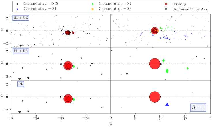
Figure 2: Event-display view of a typical two-jet event from proton–proton collision at $\sqrt{s}=13\;\text{TeV}$ at different stages of the event evolution. The respective final states are shown for various levels of soft-drop grooming, i.e. without grooming, and $z_{\text{cut}}=\{0.05,0.1,0.2,0.3\}$ with $\beta=1$.

3 NLL resummation and matching to NLO QCD

Having established the procedure for the type of observable we wish to study, we can detail the strategy for the resummation of this school of observables. In this section we will start from the general CAESAR framework for resummation and show the alterations needed for groomed event shapes. Finally, we confirm the logarithmic structure by comparing the expansion of the resummation to fixed order for groomed transverse thrust, and present matched $\text{NLO}+\text{NLL}^{\prime}$ results.

3.1 CAESAR in a nutshell

We base our calculation on the well known CAESAR formalism for soft-gluon resummation Banfi:2003je ; Banfi:2004nk . Starting from a well separated, hard Born configuration $\mathcal{B}$, it is possible to write the cumulative distribution of a given observable $v$ — resummed to NLL accuracy, with $L\equiv\ln\left(1/v\right)$ being the relevant logarithm — in a rather generic master formula

$$\begin{split}\Sigma_{\mathrm{res}}(v)&=\sum_{\delta}\Sigma^{\delta}(v)\,,\,\,\text{where}\\ \Sigma_{\mathrm{res}}^{\delta}(v)&=\int d\mathcal{B_{\delta}}\frac{\mathop{d\sigma_{\delta}}}{\mathop{d\mathcal{B_{\delta}}}}\exp\left[-\sum_{l\in\delta}R_{l}^{\mathcal{B_{\delta}}}(L)\right]\mathcal{P}^{\mathcal{B}_{\delta}}(L)\mathcal{S}^{\mathcal{B_{\delta}}}(L)\mathcal{F}^{\mathcal{B_{\delta}}}(L)\mathcal{H}^{\delta}(\mathcal{B_{\delta}})\,,\end{split}$$ (7)

and NLL is defined as systematically exponentiating all contributions of the type $\alpha_{\text{s}}^{n}L^{n}$ and higher logarithmic powers. This formulation is applicable to a wide range of observables. The sum extends over different partonic channels $\delta$; we will drop this label in the following if not explicitly needed. The main ingredients are the hard function $\mathcal{H}$ representing the kinematic cuts on the Born kinematics $\mathcal{B}$, the function $\mathcal{F}$ accounting for the effect of multiple emissions, the soft function $\mathcal{S}$ implementing the non-trivial colour evolution, the collinear radiators $R_{l}$ for all hard legs $l$, and the ratio of parton-distribution-functions (PDFs) $\mathcal{P}$ to take into account the true initial-state collinear scale,

$$\mathcal{P}^{\mathcal{B}_{\delta}}(L)=\prod_{l=1}^{2}q_{l}\left(x_{l}^{\mathcal{B_{\delta}}},e^{-L/(a_{l}+b_{l})}\mu_{F}\right)/q_{l}\left(x_{l}^{\mathcal{B_{\delta}}},\mu_{F}\right).$$ (8)

We refer to the original literature on the CAESAR formalism, in particular the review Banfi:2004yd , for a detailed discussion on the construction and the applicability of the approach. It has been used to resum a number of event shapes in hadron-hadron collisions Banfi:2010xy . These can in principle all be modified and studied as soft-drop groomed variants. We will present the general formalism to do so, we focus on groomed transverse thrust for concrete results. In what follows we make use of the implementation of the CAESAR formalism in the SHERPA framework presented originally presented in Gerwick:2014gya which we recently also applied to obtain resummed predictions for soft-drop thrust Marzani:2019evv and multijet resolution scales Baberuxki:2019ifp in electron–positron collisions.

The building blocks of the CAESAR resummation formula can be calculated for observables $V$ (vanishing at Born level) that have a specific scaling behaviour when assuming an additional soft gluon with momentum $k$, collinear to a leg $l\in\mathcal{B}$, i.e.

$$V(k)=\left(\frac{k_{t}^{\left(l\right)}}{\mu_{Q}}\right)^{a_{l}}e^{-b_{l}\eta^{\left(l\right)}}d_{l}\left(\theta\right)g_{l}\left(\phi\right)\,.$$ (9)

Here $k_{t}^{\left(l\right)}$ and $\eta^{\left(l\right)}$ are the emission’s transverse momentum and pseudorapidity relative to leg $l$, respectively. Furthermore, $\phi$ labels the azimuthal angle of the emission, while $\theta$ is the hard-process scattering angle in the centre-of-mass frame. Finally, $\mu_{Q}$ denotes the hard scale, or resummation scale, of the problem. The main goal for the remainder of this section is to recompute the building blocks including the effect of soft-drop grooming as described in Sec. 2.1.

3.2 NLL resummation for soft-drop groomed event shapes

Due to some of the complexities involved in the treatment of initial-state emissions we will compute the full resummation in the strict $v\ll z_{\text{cut}}\ll 1$ limit. This allows us to ensure that the logarithms of the observables are taken into account up to NLL accuracy. We stress that we are neglecting any contributions not associated with at least next-to-leading order in $L$, logarithms of the soft-drop parameter $z_{\text{cut}}$ are only taken into account if they appear in such a contribution. In practice the grooming logarithms are not with respect to $z_{\text{cut}}$ but some related $z_{\text{cut}}^{\prime}$ absorbing factors dependent on the exact hard kinematics, which should be taken into account for the appropriate limit instead. We will specify $z_{\text{cut}}^{\prime}$ later and just note here that, as long as $z_{\text{cut}}^{\prime}/z_{\text{cut}}={\cal O}(1)$, the two limits coincide. The region $v\sim z_{\text{cut}}$ will also not be treated and therefore the resummation will not shift into the ungroomed contribution beyond the transition point. Those effects will hence only be accounted for to the accuracy of the fixed-order calculation.

The behaviour of the observable in the presence of an additional soft gluon that remains ungroomed is still given by Eq. (9), however, grooming imposes additional phase-space constraints given by Eq. (2). Per construction, the C/A algorithm will always cluster the emission to one of the final-state legs, independent of the parton it is actually radiated off. We therefore need to treat initial- and final-state emissions separately.

In the $v\ll z_{\text{cut}}\ll 1$ limit only radiation from the final-state legs will potentially not be groomed and can result in logarithms of the observable. Collinear initial-state and the associated PDF contributions will always be groomed away and result in logarithms of $z_{\text{cut}}$ or related variables, but not be enhanced by $L$. The same is true for wide-angle soft emissions. In practice, we can hence set $R_{1}=R_{2}=0$ and $\mathcal{P}=1,\,\mathcal{S}=1$ in the groomed case. Further discussion of those contributions, relevant away from the strict limit we are working in, is presented in App. A. We finally note that this in particular includes the type of emissions with $\Delta R_{ij}\gg R_{\mathbf{SD}}$ with respect to the relevant final-state leg, which we discussed earlier due to their special nature in this approach to grooming events. Those will hence not need any special consideration in the resummed calculation at this accuracy.

Finally, in this limit the multiple-emission nature of the observable is not altered. In particular for the typical case where the multiple-emission function only depends on the logarithmic derivative of the radiator, $\mathcal{F}(L)=\mathcal{F}(R^{\prime}(L))$, we can use the same functional form as in the ungroomed case, i.e. for additive observables like transverse thrust $\mathcal{F}(R^{\prime})=e^{-\gamma_{E}R^{\prime}}/\Gamma(1+R^{\prime})$, simply with a different radiator argument. Including the limit $v\sim z_{\text{cut}}$ would change the $\mathcal{F}$ function, as discussed in detail in Appendix B.2 of Marzani:2019evv .

In the remainder of this section we will recompute the final-state leg radiators $R_{l}$. The general phase-space constraints for emissions off leg $l$ are given by:

1. (i) $\eta^{(l)}>\ln(2E_{l}/Q)$ (with $Q$ the mass of the radiating dipole) for the emission to be collinear to $l$,

2. (ii) the limit given by collinear momentum conservation, i.e. $\eta^{(l)}<\ln(2E_{l}/k_{t}^{(l)})$, and,

3. (iii) the condition $v>V(k)$, cf. left hand side of Fig. 3 for the resulting Lund-plane diagram.

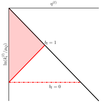
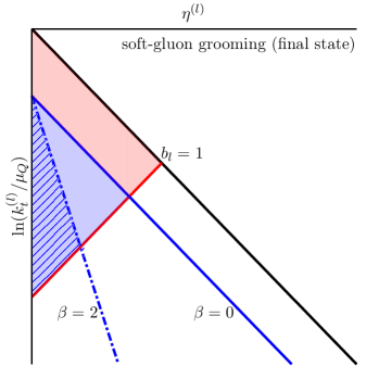
Figure 3: The emission phase space in the Lund plane illustrating the kinematic constraints without (left) and with grooming (right). In the left figure we consider the CAESAR parameters $a_{l}=1$ with $b_{l}=0$ and $b_{l}=1$ (valid for thrust). The blue areas in the right panel mark the phase-space region removed by grooming with boundaries corresponding to $\beta=0$ (solid line and area) and $\beta=2$ (dashed line, hatched area).

Soft-drop grooming now imposes an additional constraint:

1. (iv) an emission only contributes if it is not groomed, implying
   

   $$\frac{k_{t}^{(l)}e^{\left(1+\beta\right)\eta^{\left(l\right)}}}{2E_{l}}\geq z_{\text{cut}}\left(\frac{R_{\text{SD}}\sin\theta}{2}\right)^{-\beta}\equiv z_{\text{cut}}^{\prime}\,.$$

To derive this last condition, we rewrote the soft-drop criterion Eq. (2) in the soft/collinear region in terms of $k^{(l)}_{t}$ and $\eta^{\left(l\right)}$, using

$$p_{T,k}=k^{(l)}_{t}\frac{e^{\eta^{\left(l\right)}}}{2}\sin\theta\,, p_{T,l}=E_{l}\sin\theta\,,$$

$$\left|\Delta y\right|=\frac{2e^{-\eta^{\left(l\right)}}\cos\phi}{\sin\theta}\,, \left|\Delta\phi\right|=\frac{2e^{-\eta^{\left(l\right)}}\sin\phi}{\sin\theta}\,.$$

As mentioned earlier, the relevant argument of the logarithms is $z_{\text{cut}}^{\prime}$, as we now formally introduced it. It differs from $z_{\text{cut}}$ by a factor $\left(R_{\text{SD}}\mathop{\sin\theta}/2\right)^{-\beta}$. Since we are interested here in the collinear limit relative to centralised final-state particles, i.e. $\sin\theta\sim\mathcal{O}(1)$, and choose $R_{\textbf{SD}}\sim\mathcal{O}(1)$ we indeed have $z_{\text{cut}}^{\prime}/z_{\text{cut}}\sim\mathcal{O}(1)$. This implies that the limits $v\ll z_{\text{cut}}^{\prime}\ll 1$ and $v\ll z_{\text{cut}}\ll 1$ correspond to one another. In our following numerical analysis we use $R_{\textbf{SD}}=1$ and require Born-level events with $|y_{j}|<1$, cf. Eq. (5), what corresponds to $\sin\theta>0.648$. Note, the limit $z_{\text{cut}}^{\prime}\ll 1$ is challenged when considering grooming parameters $z_{\text{cut}}\geq 0.1$ and $\beta=2$. Despite this, we still probe such choices in our phenomenological analyses. However, corrections proportional to $z_{\text{cut}}^{\prime}$ beyond the ones considered here might become numerically sizeable for these cases. In any case, they will be taken into account to NLO after matching.

With the above general considerations, radiation in the blue area in the right hand side of Fig. 3 does not contribute to the groomed observable, and the integral over this area should be subtracted from the ungroomed case. This results in the radiator function for the groomed observable being given by

$$R\left(v,z_{\text{cut}}\right)=\sum_{l}C_{l} \left[\vphantom{\frac{\frac{1}{2}}{\frac{\frac{1\frac{1}{2}}{2}1}{\frac{1}{2}}}}\int_{\mu_{Q}^{2}v^{\frac{2}{a_{l}+b_{l}}}}^{\mu_{Q}^{2}}\frac{dk_{t}^{2}}{k_{t}^{2}}\frac{\alpha_{\text{s}}\left(k^{2}_{t}\right)}{\pi}\left(\ln\left(\frac{Q}{k_{t}}\right)+B_{l}\right)\right.$$

$$+ \int_{\mu_{Q}^{2}v^{\frac{2}{a_{l}}}}^{\mu_{Q}^{2}v^{\frac{2}{a_{l}+b_{l}}}}\frac{dk_{t}^{2}}{k_{t}^{2}}\frac{\alpha_{\text{s}}\left(k^{2}_{t}\right)}{\pi}\left(\ln\left(\frac{Q}{2E_{l}}\right)+\frac{1}{b_{l}}\ln\left[\left(\frac{k_{t}}{\mu_{Q}}\right)^{a_{l}}\frac{d_{l}g_{l}}{v}\right]\right)$$

$$- \int_{\mu_{Q}^{2}f\left(v,z_{\text{cut}}^{\prime}\right)}^{\mu_{Q}^{2}\left(z_{\text{cut}}^{\prime}\right)^{2}}\frac{dk_{t}^{2}}{k_{t}^{2}}\frac{\alpha_{\text{s}}\left(k^{2}_{t}\right)}{\pi}\left(\ln\left(\frac{Q}{k_{t}}\right)-\frac{\beta}{1+\beta}\ln\left(\frac{2E_{l}}{k_{t}}\right)+\frac{1}{1+\beta}\ln\left(z_{\text{cut}}^{\prime}\right)\right)$$

$$- \left.\int_{\mu_{Q}^{2}v^{\frac{2}{a_{l}}}}^{\mu_{Q}^{2}f\left(v,z_{\text{cut}}^{\prime}\right)}\frac{dk_{t}^{2}}{k_{t}^{2}}\frac{\alpha_{\text{s}}\left(k^{2}_{t}\right)}{\pi}\left(\ln\left(\frac{Q}{2E_{l}}\right)+\frac{1}{b_{l}}\ln\left[\left(\frac{k_{t}}{\mu_{Q}}\right)^{a_{l}}\frac{d_{l}g_{l}}{v}\right]\right)\right]\,,$$ (10)

with the soft-collinear corner parameterised as

$$f\left(v,z_{\text{cut}}^{\prime}\right)=v^{\frac{2\left(1+\beta\right)}{b_{l}+a_{l}\left(1+\beta\right)}}\left(z_{\text{cut}}^{\prime}\right)^{\frac{2b_{l}}{b_{l}+a_{l}\left(1+\beta\right)}}=v^{2p_{l}^{\left(v\right)}}\left(z_{\text{cut}}^{\prime}\right)^{2p_{l}^{\left(z\right)}}\,,$$ (11)

where in the second equality we defined

$$p_{l}^{(v)}\equiv\frac{1+\beta}{b_{l}+a_{l}\left(1+\beta\right)}\quad\text{and}\quad p_{l}^{(z)}\equiv\frac{b_{l}}{b_{l}+a_{l}\left(1+\beta\right)}\,.$$ (12)

The first two lines of Eq. (10) correspond to the original ungroomed triangle contribution. Using the usual CAESAR convention the coefficient $B_{l}$ accounts for hard-collinear splittings. The last two lines in Eq. (10) subtract off emissions that are groomed. The difference in the overall scales in the $k_{t}$-integration is beyond NLL accuracy and $\mu_{Q}$ can be used for all. Note that, as already indicated by our notation, we are free to use a unique scale $Q$ to represent the maximal kinematic energy available for emissions from leg $l$, although it generally differs for the contributions of the various dipoles $l$ is a part of. These differences, however, can be captured at NLL accuracy by the soft function $\mathcal{S}$, which for groomed event shapes only results in logarithms of $z_{\text{cut}}$. The radiator function can be brought to a form similar to the ungroomed case, see for instance Eq. (5) in Ref. Banfi:2003je ,

$$R\left(v,z_{\text{cut}}\right)=\sum_{l}C_{l} \left[r_{l}\left(L,\thinspace L_{z}\right)+r_{l}^{\prime}\left(L,\thinspace L_{z}\right)\left(\ln\left(\bar{d}_{l}\right)-b_{l}\ln\left(\frac{2E_{l}}{\mu_{Q}}\right)\right)\right.$$

$$\left.+\beta\,\dot{r}_{l}\left(L,\thinspace L_{z}\right)\ln\left(\frac{2E_{l}}{\mu_{Q}}\right)+B_{l}T\left(\frac{\alpha_{\text{s}}\beta_{0}L}{a_{l}+b_{l}}\right)+T\left(\alpha_{\text{s}}\beta_{0}L_{z}\right)\ln\left(\frac{Q}{\mu_{Q}}\right)\right]\,.$$ (13)

Here we have introduced an additional logarithm $L_{z}=\ln(1/z_{\text{cut}}^{\prime})$. The function $T$ is given by

$$T(X)=\int^{\mu_{Q}^{2}}_{\mu_{Q}^{2}e^{-\frac{2X}{\alpha_{\text{s}}\beta_{0}}}}\frac{dk_{t}^{2}}{k_{t}^{2}}\frac{\alpha_{\text{s}}\left(k^{2}_{t}\right)}{\pi}=\frac{-\ln(1-2X)}{\pi\beta_{0}}\,,$$ (14)

with $\beta_{0}=(11C_{A}-2n_{f})/(12\pi)$ and $\alpha_{\text{s}}=\alpha_{\text{s}}(\mu_{\text{R}}^{2})$. Furthermore, $\ln(\bar{d}_{l})$ is given by the sum of $\ln(d_{l})$ and the azimuthally averaged $\ln(g_{l})$ contribution, i.e.

$$\ln\left(\bar{d}_{l}(\theta)\right)=\ln\left(d_{l}(\theta)\right)+\int_{0}^{2\pi}\frac{d\phi}{2\pi}\ln\left(g_{l}(\phi)\right)\,.$$ (15)

The appearing resummation functions for the groomed event shapes follow the same structure as in the ungroomed case, however, the additional function $\dot{r}_{l}$ appears, given by the derivative of $r_{l}$ with respect to $L_{z}$, rather than $L$, as for $r_{l}^{\prime}$. Their explicit form reads:

$$r_{l}\left(L,\thinspace L_{z}\right) =\int_{\mu_{Q}^{2}e^{\frac{-2L}{a_{l}+b_{l}}}}^{\mu_{Q}^{2}}\frac{dk_{t}^{2}}{k_{t}^{2}}\frac{\alpha_{\text{s}}\left(k^{2}_{t}\right)}{\pi}\ln\left(\frac{\mu_{Q}}{k_{t}}\right)$$

$$+\int_{\mu_{Q}^{2}e^{-2\left(p_{l}^{\left(v\right)}L+p_{l}^{\left(z\right)}L_{z}\right)}}^{\mu_{Q}^{2}e^{\frac{-2L}{a_{l}+b_{l}}}}\frac{dk_{t}^{2}}{k_{t}^{2}}\frac{\alpha_{\text{s}}\left(k^{2}_{t}\right)}{\pi}\left(\frac{L}{b_{l}}+\frac{a_{l}}{b_{l}}\ln\left(\frac{k_{t}}{\mu_{Q}}\right)\right)$$

$$+\int_{\mu_{Q}^{2}e^{-2\left(p_{l}^{\left(v\right)}L+p_{l}^{\left(z\right)}L_{z}\right)}}^{\mu_{Q}^{2}e^{-2L_{z}}}\frac{dk_{t}^{2}}{k_{t}^{2}}\frac{\alpha_{\text{s}}\left(k^{2}_{t}\right)}{\pi}\frac{1}{1+\beta}\left(L_{z}-\ln\left(\frac{\mu_{Q}}{k_{t}}\right)\right)$$

$$=\frac{1}{\alpha_{\text{s}}}r_{1,l}\left(\alpha_{\text{s}}\beta_{0}L,\thinspace\alpha_{\text{s}}\beta_{0}L_{z}\right)+r_{2,l}\left(\alpha_{\text{s}}\beta_{0}L,\thinspace\alpha_{\text{s}}\beta_{0}L_{z}\right)\,,$$ (16)

$$r_{l}^{\prime}\left(L,\thinspace L_{z}\right) =\frac{1}{b_{l}}\int_{\mu_{Q}^{2}e^{-2\left(p_{l}^{\left(v\right)}L+p_{l}^{\left(z\right)}L_{z}\right)}}^{\mu_{Q}^{2}e^{\frac{-2L}{a_{l}+b_{l}}}}\frac{dk_{t}^{2}}{k_{t}^{2}}\frac{\alpha_{\text{s}}\left(k^{2}_{t}\right)}{\pi}$$

$$=\frac{1}{b_{l}}\left[T\left(p_{l}^{\left(v\right)}\alpha_{\text{s}}\beta_{0}L+p_{l}^{\left(z\right)}\alpha_{\text{s}}\beta_{0}L_{z}\right)-T\left(\frac{\alpha_{\text{s}}\beta_{0}L}{a_{l}+b_{l}}\right)\right]\,,$$ (17)

$$\dot{r}_{l}\left(L,\thinspace L_{z}\right) =\frac{1}{1+\beta}\int_{\mu_{Q}^{2}e^{-2\left(p_{l}^{\left(v\right)}L+p_{l}^{\left(z\right)}L_{z}\right)}}^{\mu_{Q}^{2}e^{-2L_{z}}}\frac{dk_{t}^{2}}{k_{t}^{2}}\frac{\alpha_{\text{s}}\left(k^{2}_{t}\right)}{\pi}$$

$$=\frac{1}{1+\beta}\left[T\left(p_{l}^{\left(v\right)}\alpha_{\text{s}}\beta_{0}L+p_{l}^{\left(z\right)}\alpha_{\text{s}}\beta_{0}L_{z}\right)-T\left(\alpha_{\text{s}}\beta_{0}L_{z}\right)\right]\,.$$ (18)

The LL and NLL terms $r_{1,l}$ and $r_{2,l}$ appearing in Eq. (16) are given by

$$r_{1,l}\left(\lambda,\thinspace\lambda_{z}\right)=\frac{-1}{2\pi\beta_{0}^{2}} \left[\frac{a_{l}+b_{l}}{b_{l}}\left(1-\frac{2\lambda}{a_{l}+b_{l}}\right)\ln\left(1-\frac{2\lambda}{a_{l}+b_{l}}\right)+\frac{1}{1+\beta}\left(1-2\lambda_{z}\right)\ln\left(1-2\lambda_{z}\right)\right.$$

$$-\left.\frac{a_{l}(1+\beta)+b_{l}}{b_{l}(1+\beta)}\left(1-2(p_{l}^{\left(v\right)}\lambda+p_{l}^{\left(z\right)}\lambda_{z})\right)\ln\left(1-2(p_{l}^{\left(v\right)}\lambda+p_{l}^{\left(z\right)}\lambda_{z})\right)\right]\,,$$ (19)

$$r_{2,l}\left(\lambda,\thinspace\lambda_{z}\right)=\frac{K}{4\pi^{2}\beta_{0}^{2}} \left[\frac{a_{l}+b_{l}}{b_{l}}\ln\left(1-\frac{2\lambda}{a_{l}+b_{l}}\right)+\frac{1}{1+\beta}\ln\left(1-2\lambda_{z}\right)\right.$$

$$\left.-\frac{a_{l}(1+\beta)+b_{l}}{b_{l}(1+\beta)}\ln\left(1-2(p_{l}^{\left(v\right)}\lambda+p_{l}^{\left(z\right)}\lambda_{z})\right)\right]$$

$$-\frac{\beta_{1}}{2\pi\beta_{0}^{3}} \left[\frac{a_{l}+b_{l}}{b_{l}}\left(\frac{1}{2}\ln^{2}\left(1-\frac{2\lambda}{a_{l}+b_{l}}\right)+\ln\left(1-\frac{2\lambda}{a_{l}+b_{l}}\right)\right)\right.$$ (20)

$$\left.+\frac{1}{1+\beta}\left(\frac{1}{2}\ln^{2}\left(1-2\lambda_{z}\right)+\ln\left(1-2\lambda_{z}\right)\right)\right.$$

$$\left.-\frac{a_{l}(1+\beta)+b_{l}}{b_{l}(1+\beta)}\left(\frac{1}{2}\ln^{2}\left(1-2(p_{l}^{\left(v\right)}\lambda+p_{l}^{\left(z\right)}\lambda_{z})\right)+\ln\left(1-2(p_{l}^{\left(v\right)}\lambda+p_{l}^{\left(z\right)}\lambda_{z})\right)\right)\right]\,,$$

with the coefficient $K$ in the $\overline{\text{MS}}$ renormalisation scheme given by $K=\left(\frac{67}{18}-\frac{\pi^{2}}{6}\right)C_{A}-\frac{5}{9}n_{f}$. In order to perform the actual calculation of the resummation we extended the SHERPA resummation plugin Gerwick:2014gya to include the soft-drop groomed version of the final-state radiators as presented above.

3.3 The non-perturbative realm

As is the case in the original CAESAR formalism, cf. also Luisoni:2015xha , the formulae presented here exhibit logarithmic branch cuts as a result of integrating the strong-coupling constant over the Landau pole. The positions of these branch cuts can be used to estimated the observable scales at which non-perturbative physics, i.e. hadronisation effects, dominate. From Eqs. (19) and (20) we can read off their locations as

$$2\lambda =a_{l}+b_{l}\,,$$ (21)

$$2p_{l}^{\left(v\right)}\lambda =1-2p_{l}^{\left(z\right)}\lambda_{z}\,.$$ (22)

Here we assumed $\lambda_{z}<1/2$. These can easily be expressed in terms of the observable $v=e^{-\lambda/\alpha_{\text{s}}\beta_{0}}$, which yields

$$v_{\text{Had, collinear}} =\left(e^{-1/2\alpha_{\text{s}}\beta_{0}}\right)^{a_{l}+b_{l}}=\left(\frac{\Lambda_{\text{QCD}}}{\mu_{R}}\right)^{a_{l}+b_{l}}\,,$$ (23)

$$v_{\text{Had, wide-angle}} =\left(e^{-1/2\alpha_{\text{s}}\beta_{0}}\right)^{a_{l}+b_{l}/(1+\beta)}\left(e^{L_{z}}\right)^{b_{l}/(1+\beta)}=\left(\frac{\Lambda_{\text{QCD}}}{\mu_{R}}\right)^{a_{l}}\left(\frac{\Lambda_{\text{QCD}}}{\mu_{R}z_{\text{cut}}^{\prime}}\right)^{b_{l}/(1+\beta)}\,.$$ (24)

For the last equality we introduced $\Lambda_{\text{QCD}}^{2}=\mu_{R}^{2}e^{-1/\alpha_{\text{s}}\beta_{0}}$. The notation reflects that the first solution corresponds to the collinear limit, whereas the second one is approached for the softest wide-angle emissions allowed by grooming (i.e. the intersection of the blue and red line in Fig. 3). The condition on $\lambda_{z}$ translates to $z_{\text{cut}}^{\prime}>\Lambda_{\text{QCD}}/\mu_{R}$, which if violated puts the full groomed part of the distribution into the non-perturbative region. Hadronisation corrections start to dominate when $v$ approaches the larger of the two solutions, such that, keepint in mind $\beta\geq 0$, we have

$$v_{\text{Had}} =\left(\frac{\Lambda_{\text{QCD}}}{\mu_{R}}\right)^{a_{l}+b_{l}}\,,\qquad\text{for }~{}b_{l}\leq 0\,,$$ (25)

$$v_{\text{Had}} =\left(\frac{\Lambda_{\text{QCD}}}{\mu_{R}}\right)^{a_{l}}\left(\frac{\Lambda_{\text{QCD}}}{\mu_{R}z_{\text{cut}}^{\prime}}\right)^{b_{l}/(1+\beta)}\,,\qquad\text{for }~{}b_{l}>0\,.$$ (26)

This agrees with the estimates given for example in Refs. Frye:2016aiz ; Caletti:2021oor for the energy-energy correlations $e_{2}^{(\alpha)}$ and jet angularities $\lambda^{1}_{\alpha}$, where the relevant parameters are $a_{l}=1$, $b_{l}=\alpha-1$ (see the latter reference for a detailed treatment using the CAESAR parametrisation). For reference, we note that, without grooming (i.e. $\beta\to\infty$), we would obtain

$$v^{\text{ungroomed}}_{\text{Had}}=\left(\frac{\Lambda_{\text{QCD}}}{\mu_{R}}\right)^{a_{l}}\,,\qquad\text{for }~{}b_{l}>0\,,$$ (27)

while the $b_{l}\leq 0$ case remains unchanged since here the dominant contribution is from the collinear limit. By comparing Eqs. (26) and (27) it is apparent that grooming reduces the impact of hadronisation corrections.

In Fig. 4 we present concrete results for $v_{\text{Had}}$ for different combinations of CAESAR observable parameters in dependence on the dimensionless ratio $\mu_{\text{R}}/\Lambda_{\text{QCD}}$. The black solid line corresponds to the case $a_{l}=1$ and $b_{l}=-1/2$, representing, for example, the so-called LHA jet angularity $\lambda^{1}_{1/2}$. As stated above, for observables with $b_{l}<0$ the onset of hadronisation dominance is, independent of grooming, given by Eq. (25). As also noted in Ref. Caletti:2021oor , this observable is very susceptible to non-perturbative corrections, even for rather high values of $\mu_{\text{R}}$. The black dashed line represents the class of observables parametrised by $a_{l}=1$ and $b_{l}\geq 0$ for the case of no grooming. Compared to the LHA angularity a somewhat reduced sensitivity to hadronisation effects is evident. However, this can be significantly reduced through soft-drop grooming. This is exemplified for the parameter set $a_{l}=b_{l}=1$, corresponding to the thrust observable we are going to study in what follows. We consider here grooming with $\beta\in\{0,1,2\}$ and two representative $z_{\text{cut}}^{\prime}$ values, i.e. $z_{\text{cut}}^{\prime}\in\{0.1,0.2\}$. For the considered range of $\mu_{\text{R}}/\Lambda_{\text{QCD}}$ grooming with $\beta=2$ reduces the transition point $v_{\text{Had}}$ by about $1-2$ $e$-folds. However, the dependence on $z_{\text{cut}}^{\prime}$ is rather mild. As evident from Eq. (26), the strongest suppression is obtained for $\beta=0$. For $z_{\text{cut}}^{\prime}=0.1$ $v_{\text{Had}}$ gets reduced by about $4$ $e$-folds at $\mu_{\text{R}}/\Lambda_{\text{QCD}}=1000$. By increasing $z_{\text{cut}}^{\prime}$ to $0.2$ we roughly gain another factor of $e$.

While these estimates are certainly helpful in getting a feeling for the ultimate breakdown of the perturbative approach, we note that they do not provide information on the scales related to the underlying event. In Sec. 4 such effects are addressed in a phenomenological study.

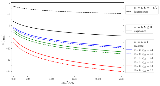
Figure 4: Observable value $v_{\text{Had}}$ where to expect dominance of non-perturbative corrections, i.e. hadronisation effects, as a function of the dimensionless quantity $\mu_{\text{R}}/\Lambda_{\text{QCD}}$. Results are given for different combinations of CAESAR parameters. For the case $a_{l}=b_{l}=1$, relevant for example for the thrust observable, we present results for different grooming parameter combinations.

3.4 Matching to NLO and achieving $\text{NLL}^{\prime}$ accuracy

We improve the pure resummation by matching to a fixed-order calculation at NLO QCD, i.e. at ${\cal{O}}(\alpha_{\text{s}}^{2})$ relative to the Born process. We combine our NLL resummation and the NLO in a way that allows us to effectively achieve $\text{NLL}^{\prime}$ accuracy. In what follows we detail our approach and discuss subtleties arising due to soft-drop grooming.

Preliminaries

Before performing the actual calculation it is common to exploit the ambiguities present at NLL to ease the matching to a fixed-order result. The natural argument of the logarithms $L_{z}$ is the value of the transition point for these types of emissions. Naturally, grooming vanishes as $v\to\left(z_{\text{cut}}^{\prime}\right)^{a_{l}}$, at which point the observable transitions back to the ungroomed case. However, this is based on the NLL approximation of the kinematics. Formally, in the Lund plane the LO transition point is reached when the intersection of the $\eta^{(l)}=\ln(2E_{l}/Q)$ line and the soft-drop line is at the same value of $k_{t}$ as that with the observable line. When this occurs the soft-drop line no longer results in a kinematic boundary on the emissions and instead the observable value is the only constraint. This happens when:

$$z_{\text{cut}}^{\prime}Q^{1+\beta}\left(2E_{l}\right)^{-\beta}=\left(\frac{v_{\text{trans}}}{d_{l}g_{l}}\right)^{1/a_{l}}\left(\frac{2E_{l}}{Q}\right)^{b_{l}/a_{l}}\mu_{Q}\,,$$ (28)

resulting in the transition point

$$v_{\text{trans}}=\left(z_{\text{cut}}^{\prime}\right)^{a_{l}}\left(\frac{2E_{l}}{\mu_{Q}}\right)^{a_{l}}\left(\frac{Q}{2E_{l}}\right)^{a_{l}\left(1+\beta\right)+b_{l}}d_{l}g_{l}=\tilde{z}_{\text{cut}}^{a_{l}}\,.$$ (29)

At fixed logarithmic accuracy we can always shift the argument of the logarithms by multiplying $z_{\text{cut}}^{\prime}$ with a constant and include an additional contribution to compensate for the leading terms in $L_{z}$. This way we can make use of the actual LO transition point for this type of emission as an argument of the logarithm, by comparing the full relations instead of the NLL approximation. Accordingly, we shift the argument of the logarithm from $L_{z}=-\ln(z_{\text{cut}}^{\prime})\to-\ln(\tilde{z}_{\text{cut}})$, and the additional contribution that needs to be taken into account reads:

$$R\to R+\frac{1}{a_{l}}\dot{r}_{l}\left(L,\thinspace L_{z}\right)\left[a_{l}\ln\left(\frac{2E_{l}}{\mu_{Q}}\right)+\left(a_{l}\left(1+\beta\right)+b_{l}\right)\ln\left(\frac{Q}{2E_{l}}\right)+\ln\left(\bar{d}_{l}\right)\right]\,.$$ (30)

Next, we include end-point corrections Catani:1992ua ; Jones:2003yv to ensure the cumulative distribution of the resummation approaches unity and its derivative vanishes at the kinematic end-point of the fixed-order distribution. Two types of logarithms are included, the one of the observable, which can be altered to vanish at the end-point, and logarithms of $z_{\text{cut}}$, which will not vanish there. The observable logarithms are modified in the usual manner

$$\ln\left(\frac{1}{x_{L}v}\right)\to\frac{1}{p}\ln\left(\frac{1}{\left(x_{L}v\right)^{p}}-\frac{1}{\left(x_{L}v^{\mathrm{max}}\right)^{p}}+1\right)=L\,,$$ (31)

where $x_{L}$ is chosen to be

$$\ln(x_{L})=-\sum_{l\in f}\ln(\bar{d}_{l})/n\,,$$ (32)

see Ref. Baberuxki:2019ifp , averaged over the final-state particles only, here $n=2$. Per default we will assume $p=1$. The argument of logarithms of $z_{\text{cut}}$ we multiply by the same factor, i.e. $L_{z}=-\ln(x_{L}\tilde{z}_{\text{cut}}^{a_{l}})/a_{l}$. Finally the exponential is modified according to

$$\exp\left[\tilde{R}\left(L,\,L_{z}\right)\right]\to\exp\left[\tilde{R}\left(L,\,L_{z}\right)-\tilde{R}\left(0,\,L_{z}\right)-\left(\frac{v}{v^{\text{max}}}\right)^{p}\tilde{R}^{\prime}\left(0,\,L_{z}\right)L\right],$$ (33)

where $\tilde{R}$ includes the multiple-emission function $\mathcal{F}$, and $\tilde{R}^{\prime}$ is its derivative with respect to $L$. Here we subtract $\tilde{R}\left(0,\,L_{z}\right)$ to consistently remove all pure $L_{z}$ type of contributions.

To remind the reader, for the practical implementation we focus on the resummation of logarithms in the observable in the strict limit $v\ll z_{\text{cut}}\ll 1$. Therefore we shall neglect the transition point in the resummation and expansion. We will only perform the exponentiation of the logarithms of the groomed observable, which requires the inclusion of final-state emissions only in the exponential. Other contributions result in logarithms of $z_{\text{cut}}$ and will be included through means of matching to fixed order, i.e. NLO QCD.

Definition of the matched distributions

To match the resummed predictions to the fixed-order calculation, we follow the strategy presented using our conventions in Baberuxki:2019ifp . We adopt the same notation, i.e. for every partonic channel $\delta$ we introduce the cumulant distributions

$$\Sigma^{\delta}(v)=\int_{0}^{v}\mathop{d\sigma^{\delta}}\quad\text{and}\quad\overline{\Sigma}^{\delta}(v)=\int_{v}^{1}\mathop{d\sigma^{\delta}}\,,$$ (34)

both, for the resummed (res) and the fixed-order (fo) calculations. They can be expanded in $\alpha_{\text{s}}$ relative to the Born configuration, which itself is ${\cal{O}}(\alpha_{\text{s}}^{2})$,

$$\Sigma^{\delta}(v)=\sigma^{\delta,(0)}+\Sigma^{\delta,(1)}(v)+\Sigma^{\delta,(2)}(v)+\dots~{},\;\;\text{where}\;\;\Sigma^{\delta,(n)}(v)\propto\alpha_{\text{s}}^{n+2}~{},$$ (35)

and $\sigma^{\delta,(0)}=\Sigma^{\delta,(0)}(1)$. We then define (taking the argument of the cumulants as implicit) the multiplicatively matched cumulant distribution for channel $\delta$

$$\Sigma^{\delta}_{\mathrm{mult}} =\Sigma^{\delta}_{\mathrm{res}}\left[1+\frac{\Sigma^{\delta,(1)}_{\mathrm{fo}}-\Sigma^{\delta,(1)}_{\mathrm{res}}}{\sigma^{\delta,(0)}}+\frac{1}{\sigma^{\delta,(0)}}\left(-\overline{\Sigma}^{\delta,(2)}_{\mathrm{fo}}-\Sigma^{\delta,(2)}_{\mathrm{res}}-\frac{\Sigma^{\delta,(1)}_{\mathrm{res}}}{\sigma^{\delta,(0)}}\left(\Sigma^{\delta,(1)}_{\mathrm{fo}}-\Sigma^{\delta,(1)}_{\mathrm{res}}\right)\right)\right]\,,$$ (36)

which reproduces the fixed-order result when expanded to ${\cal{O}}(\alpha_{\text{s}}^{2})$. In the limit $v\to 0$ it reduces to

$$\Sigma_{\mathrm{mult}}^{\delta}\to\left(1+\frac{\alpha_{\text{s}}}{2\pi}C_{1}^{\delta}+{\cal{O}}(\alpha_{\text{s}}^{2})\right)\Sigma_{\mathrm{res}}^{\delta}~{},\;\;\text{where}\qquad\frac{\alpha_{\text{s}}}{2\pi}C_{1}^{\delta}\equiv\lim_{v\to 0}\frac{\Sigma^{\delta,(1)}_{\mathrm{fo}}-\Sigma^{\delta,(1)}_{\mathrm{res}}}{\sigma^{\delta,(0)}}\,.$$ (37)

We later also refer to matched distributions at LO, which corresponds to including in Eq. (36) only the first two terms in the square brackets. Finally, the full cumulative distribution is given by the sum over partonic channels, i.e.

$$\Sigma_{\mathrm{match}}=\sum_{\delta\in\mathcal{B}}\Sigma_{\mathrm{match}}^{\delta}+\sum_{\delta\notin\mathcal{B}}\Sigma^{\delta}_{\mathrm{fo}}\,,$$ (38)

where the second sum takes into account channels vanishing in the soft limit and hence not part of the resummation.

Channel separation

In order to separate the fixed-order phase space into the different channels $\delta$, we employ the ‘flavour-$k_{t}$’ algorithm defined in Banfi:2006hf , called BSZ algorithm in the following. This is the approach taken in the resummation of plain event shapes at hadron colliders in Banfi:2010xy . We implemented and used the lepton-collider variant of this algorithm in our framework in earlier work Baberuxki:2019ifp . Here we will need to consider the hadron-collider version. We obtain the fixed-order matrix elements from the COMIX generator Gleisberg:2008fv , that provides all the required information about the flavour assignment of initial- and final-state partons in an automated fashion. The BSZ algorithm constitutes a sequential recombination algorithm, where the particle $i$ with the smallest distance measure

$$d_{ij} =\begin{cases}\min\left(p^{2}_{T,i},p^{2}_{T,j}\right)\Delta R^{2}_{ij}\,,&\text{if softer of $i,j$ is a gluon}\\ \max\left(p^{2}_{T,i},p^{2}_{T,j}\right)\Delta R^{2}_{ij}\,,&\text{if softer of $i,j$ is a quark}\end{cases},~{}$$ (39)

$$d_{iB} =\begin{cases}\min\left(p^{2}_{T,i},p^{2}_{T,B}(y_{i})\right)\,,&\text{if $i$ is a gluon}\\ \max\left(p^{2}_{T,i},p^{2}_{T,B}(y_{i})\right)\,,&\text{if $i$ is a quark}\end{cases}\,,\quad$$ (40)

$$d_{i\overline{B}} =\begin{cases}\min\left(p^{2}_{T,i},p^{2}_{T,\overline{B}}(y_{i})\right)\,,&\text{if $i$ is a gluon}\\ \max\left(p^{2}_{T,i},p^{2}_{T,\overline{B}}(y_{i})\right)\,,&\text{if $i$ is a quark}\end{cases},~{}$$ (41)

where $$\quad\begin{array}[]{l}p_{T,B}(y)=\sum_{j}p_{T,j}\left(\Theta\left(y_{j}-y\right)+\Theta\left(y-y_{j}\right)e^{y_{j}-y}\right)\\ p_{T,\overline{B}}(y)=\sum_{j}p_{T,j}\left(\Theta\left(y-y_{j}\right)+\Theta\left(y_{j}-y\right)e^{y-y_{j}}\right)\end{array}\,,$$ (44)

is combined with either final-state particle $j$ or the forward ($B$) or backward ($\overline{B}$) beam. The flavour of the combined object is determined by the sum of the flavours of the two clustered entities. For this purpose, any object with (anti-)quark flavour is called a quark, a gluon is an object without any net flavour (including the case of same-flavour quark-antiquark pairs). We run this algorithm until only two final-state objects are left. Together with the initial state, their flavours define the channel $\delta$ to which we assign the event. The algorithm as described so far can lead to channels that are not present as Born channels, e.g. including objects that have multiple (anti-)quarks or anti-quarks and quarks of different flavour associated to them. In our matching scheme they are taken into account in the sum over $\delta\notin\mathcal{B}$ in Eq. (38). We collect all those configurations in a common channel, denoted as ‘other’. To test the infrared safety of the BSZ algorithm and our implementation we need to check that this channel vanishes in the soft limit, i.e. if all but two particles become soft and/or collinear to one of the two remaining particles. This validation is presented in Fig. 5. We use transverse thrust $\tau_{\perp}$ as a measure for the hardness of the event. Infrared safety then implies that the differential cross section for the ‘other’ channel approaches zero in the limit $\tau_{\perp}\to 0$.

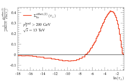
Figure 5: The ${\cal{O}}(\alpha_{\text{s}}^{2})$ contribution to the ‘other’ channel in the limit $\tau_{\perp}\to 0$.

For the results we present in this work, we will use what is referred to as ‘bland’ version of the BSZ algorithm in Banfi:2006hf , i.e., we veto any clustering that would lead to such not Born like jets, by effectively setting the measure $d_{ij}$ (and likewise the beam distance measures) to infinity for those cases.

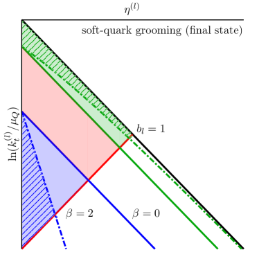
Figure 6: Left: The emission phase space in the Lund plane with the CAESAR parameters $a_{l}=1$ and $b_{l}=1$ (valid for thrust). The green area marks the phase-space region where the emitting particle will be removed by grooming with boundaries corresponding to $\beta=0$ (solid line and area) and $\beta=2$ (dashed line, hatched area). The blue area marks the region where the emitted gluon is removed, cf. Fig. 3. Right: Displays of the transverse plane of several LO final-state configurations. The colour codes indicate jet association according to the BSZ algorithm, groomed particles are in light shade and dashed in the case of quarks. (a) Sample event from the green area, where the quark is groomed instead of the gluon. (b), (c) Sample events with two quarks in one hemisphere, with the softer one getting groomed, for different jet clusterings. (d) Sample event from the blue area, a soft gluon is groomed.

$C_{1}^{\delta}$ and $\text{NLL}^{\prime}$ accuracy for soft-drop event shapes

The matching scheme we use in principle provides the correct constant $C_{1}^{\delta}$ up to terms beyond $\text{NLL}^{\prime}$ due to implicit averaging over different Born kinematics, see also the discussion in Banfi:2010xy ; Baberuxki:2019ifp . However, some subtleties arise, as the application of soft-drop grooming implies that the limit $v^{\text{SD}}\to 0$ does not uniquely impose the soft limit for all particles beyond the Born multiplicity. Hence $\Sigma^{\delta,(1)}_{\mathrm{fo}}$ in this limit consists of several pieces. As usual, there is the constant contribution of the virtual-real corrections at $v^{\text{SD}}=0$ and, for the real correction, there is a part of phase space where nothing is groomed, contributing a finite remainder between the integral of this phase space and $\Sigma^{\delta,(1)}_{\mathrm{res}}$. The pieces additionally present due to grooming are real corrections that result in $v^{\text{SD}}=0$ due to one particle being groomed away. In principle those should be multiplied by the appropriate Sudakov factors for the corresponding $(n+1)$-particle final state. However, to achieve $\text{NLL}^{\prime}$ accuracy those are needed at LL only, i.e. only in the limit of radiation that is simultaneously soft and collinear. This results in the same factor as for the $2\to 2$ configuration obtained by ignoring the groomed parton.

In practice, we sort all events according to the BSZ  cluster algorithm described above. A groomed gluon in a LO event will always also be clustered first, since it will have the smallest transverse momentum overall and the remaining two particles can not be collinear due to momentum conservation in the transverse plane. A configuration like this is shown in Fig. 6 in panel (d). For a gluon, the flavour assignment from this algorithm is hence the same as if it was simply discarded. This is still the case if a groomed quark is clustered to the beam, since our soft-drop observables are insensitive to initial-state radiation at LL. However, this will no longer be the case if a quark is groomed away but clustered to another final-state parton. This can happen if two quarks are in the same hemisphere. This is illustrated in panels (b) and (c) of Fig. 6, which would be classified as quark-quark (b) and gluon-gluon (c) like final states. Finally, a quark can be in a hemisphere together with a gluon, but be softer. The corresponding configuration in panel (a) of Fig. 6 would be attributed to the quark-quark channel. However, all those cases are suppressed with powers of $z_{\text{cut}}$. Since we work in the limit $z_{\text{cut}}\ll 1$, those terms are beyond our accuracy target. The phase-space region where this happens is illustrated in the left part of Fig. 6. For $\beta=0$, these power corrections are logarithmically enhanced and need to be taken into account at NLL accuracy if finite $z_{\text{cut}}$ effects are important, cf. Dasgupta:2013ihk ; Marzani:2017mva . With $\beta>0$, they still provide a constant contribution which would enter at $\text{NLL}^{\prime}$ accuracy. We note that, despite being formally irrelevant for us, these phase-space regions might still be problematic from a practical point of view when matching NLO and NLL resummation as we do here. This is due to flavour assignments that have no corresponding Born process and would thus be assigned to the ‘other’ channel. These are not guaranteed to vanish in the $v^{\text{SD}}\to 0$ limit (infrared safety of the flavour algorithm of course mandates that this happens in the $v\to 0$ limit, as we demonstrated above for $v=\tau_{\perp}$). This could lead to an unphysical behaviour where the matched distribution approaches a finite constant rather than zero in the soft limit. This could be solved by adjusting details of the matching scheme. However, we do not encounter this problem as we use the ‘bland’ variant of the BSZ algorithm.

With the above discussion at hand, we can conclude that our calculations achieve $\text{NLO}+\text{NLL}^{\prime}$ accuracy, in the $z_{\text{cut}}\ll 1$ limit, for histograms of differential distributions, scaled by the overall cross section at the corresponding accuracy, i.e.

$$\frac{1}{\sigma}\frac{\mathop{d\sigma}}{\mathop{d\ln(v^{\text{SD}})}}\equiv\frac{1}{\Sigma_{\mathrm{match}}(1)}\frac{\mathop{d\Sigma_{\mathrm{match}}(v^{\text{SD}})}}{\mathop{d\ln(v^{\text{SD}})}}\,.$$ (45)

3.5 Results for soft-drop transverse thrust

Here we apply our resummation for soft-drop groomed hadronic event shapes for the transverse-thrust observable introduced in Eq. (3). The parameters of its CAESAR representation, cf. Eq. (9), are collected in Table 1. In addition, in Table 2 we list the kinematic end-point values $v^{\text{max}}$, extracted from fixed-order calculations, for the ungroomed observable and those cases where grooming actually limits the observable range.

$\tau_{\perp}$	$a_{l}$	$b_{l}$	$d_{l}(\theta)$	$g_{l}(\phi)$
$l\in$ initial state	1	0	$\frac{1}{\sin\theta}\left(\frac{\mu_{Q}}{Q_{12}}\right)$	$1-\left|\cos\phi\right|$
$l\in$ final state	1	1	$\frac{1}{\sin^{2}\theta}\left(\frac{\mu_{Q}}{Q_{12}}\right)$	$\sin^{2}\phi$

Table 1: The CAESAR parametrisation valid for both plain and soft-drop groomed transverse thrust, given for initial- and final-state hard-process legs.

$z_{\text{cut}}\vphantom{\frac{\frac{12}{1}}{2}}$	$\beta$	$v^{\text{max}}_{\text{LO}}$	$v^{\text{max}}_{\text{NLO}}$
Ungroomed		$1/3$	0.3406
0.2	2	0.2927	0.3067
0.3	1	0.2929	0.3067
0.3	2	0.1994	0.2174

Table 2: Table of transverse thrust end-point values determined numerically at LO and NLO. The kinematical end-points for the $\beta,z_{\text{cut}}$ values not shown are unaltered by grooming.

All phase-space integrals are performed using SHERPA Gleisberg:2008ta ; Bothmann:2019yzt . This includes the integration over the Born phase space in Eq. (7), and, over the three- and four-particle phase space needed to evaluate the cumulants at LO and NLO QCD. For the LO, i.e. the calculation of $\Sigma_{\mathrm{fo}}^{(1)}(v^{\text{SD}})$, we need to add the constant contribution from the virtual correction to the Born $2\to 2$ parton scattering process and the real correction integrated up to $\tau_{\perp}^{\text{SD}}=v^{\text{SD}}$. Both parts are regularised using Catani–Seymour dipole subtraction Catani:1996vz ; Gleisberg:2007md . We obtain the required one-loop virtual matrix elements from OPENLOOPS Cascioli:2011va , using the COLLIER library Denner:2016kdg for the evaluation of tensor and scalar integrals. For the NLO calculation we regulate double real-correction divergences in the infrared by requiring $\tau_{\perp}>\tau^{\text{cut}}_{\perp}$. This implies that we do not need to calculate the two-loop virtual corrections, for which $\tau_{\perp}=0$. In the remaining phase space, the $2\to 3$ parton matrix element is finite (though possibly numerically large close to the cutoff), and we can evaluate the one-loop virtual and real corrections, including one real emission that might be arbitrarily soft/collinear, using the same tools as in the LO case. Since our matching formula Eq. (36) only depends on $\overline{\Sigma}_{\mathrm{fo}}^{(2)}(v^{\text{SD}})$, which is an integral from $v^{\text{SD}}$ to $1$, see Eq. (34), our final results are independent of the infrared cut for $v^{\text{SD}}>\tau^{\text{cut}}_{\perp}$. Using the fact that the value of groomed transverse thrust is strictly smaller than the corresponding value of ungroomed thrust, we can generate all results by setting the cut in $\tau_{\perp}$ to the lowest observable value we are interested in. In practice, we use $\tau^{\mathrm{cut}}_{\perp}=e^{-11}\approx 1.7\times 10^{-5}$.

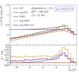
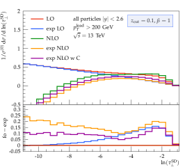
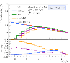
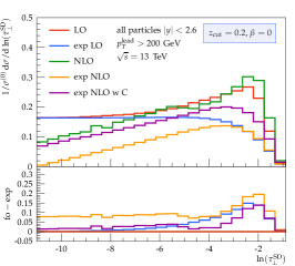
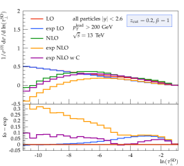
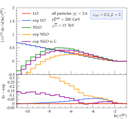
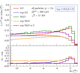
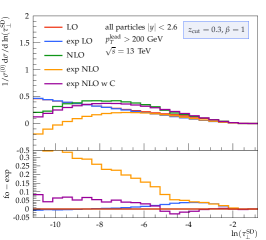
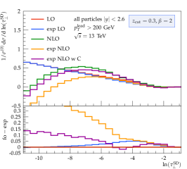
Figure 7: Comparison of the expansion of the NLL resummation and fixed-order results for soft-drop groomed thrust at LO and NLO accuracy. The lower panels show the difference between expansion and fixed order at LO and NLO.

For our calculation, the factorisation, renormalisation and resummation scale are chosen identical and equal to half the scalar sum of the partonic transverse momenta, i.e.

$$\mu_{\text{R}}=\mu_{\text{F}}=\mu_{\text{Q}}=\frac{1}{2}H_{T}\,.$$ (46)

We make use of the NNPDF-3.0 NNLO PDF Ball:2014uwa and evaluate $\alpha_{\text{s}}(\mu_{\text{R}}^{2})$ at two-loop starting from $\alpha_{\text{s}}(M^{2}_{Z})=0.118$, with a fixed number of $n_{f}=5$ active flavours.

In Fig. 7 we compile fixed-order results for the $p_{T,\text{min}}=200\;\text{GeV}$ event selection for different combinations of grooming parameters. Alongside we show the expansions of our resummation formulae to LO and NLO in $\alpha_{\text{s}}$. Note, our NLO results are in fact independent of the infrared regulator $\tau^{\mathrm{cut}}_{\perp}$ since $\frac{\mathop{d\Sigma}(v^{\text{SD}})}{\mathop{dv^{\text{SD}}}}=-\frac{\mathop{d\overline{\Sigma}}(v^{\text{SD}})}{\mathop{dv^{\text{SD}}}}$, cf. Eq. (34). In the notation of the previous section, we compare the derivatives $\frac{\mathop{d\Sigma}}{\mathop{d\ln\tau_{\perp}^{\text{SD}}}}$ of the cumulative distributions at LO

$$\Sigma_{\text{LO}}(\tau_{\perp}^{\text{SD}}) =\sum_{\delta}\left(\sigma^{\delta,(0)}+\Sigma_{\mathrm{fo}}^{\delta,(1)}(\tau_{\perp}^{\text{SD}})\right)\,,$$ (47)

$$\Sigma_{\text{exp LO}}(\tau_{\perp}^{\text{SD}}) =\sum_{\delta}\left(\sigma^{\delta,(0)}+\Sigma_{\mathrm{res}}^{\delta,(1)}(\tau_{\perp}^{\text{SD}})\right)\,,$$ (48)

and at NLO

$$\Sigma_{\text{NLO}}(\tau_{\perp}^{\text{SD}}) =\sum_{\delta}\left(\sigma^{\delta,(0)}+\Sigma_{\mathrm{fo}}^{\delta,(1)}(\tau_{\perp}^{\text{SD}})-\overline{\Sigma}^{\delta,(2)}_{\mathrm{fo}}(\tau_{\perp}^{\text{SD}})\right)\,,$$ (49)

$$\Sigma_{\text{exp \text{NLO}}}(\tau_{\perp}^{\text{SD}}) =\sum_{\delta}\left(\sigma^{\delta,(0)}+\Sigma_{\mathrm{res}}^{\delta,(1)}(\tau_{\perp}^{\text{SD}})+\Sigma^{\delta,(2)}_{\mathrm{res}}(\tau_{\perp}^{\text{SD}})\right)\,,$$ (50)

$$\Sigma_{\text{exp \text{NLO}}}^{C}(\tau_{\perp}^{\text{SD}}) =\sum_{\delta}\left(\sigma^{\delta,(0)}+\left(1+\frac{\Sigma_{\mathrm{fo}}^{\delta,(1)}(\tau_{\perp}^{\text{SD}})-\Sigma_{\mathrm{res}}^{\delta,(1)}(\tau_{\perp}^{\text{SD}})}{\sigma^{\delta,(0)}}\right)\Sigma_{\mathrm{res}}^{\delta,(1)}(\tau_{\perp}^{\text{SD}})+\Sigma^{\delta,(2)}_{\mathrm{res}}(\tau_{\perp}^{\text{SD}})\right)\,,$$ (51)

where the last definition corresponds to the inclusion of $C_{1}^{\delta}$ in the expansion in the limit $\tau_{\perp}^{\text{SD}}\to 0$. For all considered grooming parameters, we observe that the subtractions of the LO results, i.e. $\frac{\mathop{d}}{\mathop{d\ln\tau_{\perp}^{\text{SD}}}}\left(\Sigma_{\text{LO}}-\Sigma_{\text{exp LO}}\right)$, tend to zero as $\tau_{\perp}^{\text{SD}}\to 0$ (blue lines), confirming that all logarithmically enhanced terms are correctly captured by the expansion. In the difference between the exact NLO results and the naive expansion, $\Sigma_{\text{NLO}}-\Sigma_{\text{exp \text{NLO}}}$, for $\beta>0$ we expect and observe residual single-logarithmic contributions $\propto{\cal{O}}(1)\alpha_{\text{s}}^{2}L^{2}$, i.e. a linear rising difference in the derivative $\frac{\mathop{d}}{\mathop{d\ln\tau_{\perp}^{\text{SD}}}}\left(\Sigma_{\text{NLO}}-\Sigma_{\text{exp \text{NLO}}}\right)$ (orange lines). This contribution is a cross term between the $C^{\delta}_{1}$ coefficients and the LL $\alpha_{\text{s}}L^{2}$ contribution. However, as the LO structure for $\beta=0$ starts at $\alpha_{\text{s}}L$, this cross term does not exist for this case and the first order at which there is a difference is ${\cal{O}}(1)\alpha_{\text{s}}^{2}L$. In addition there are finite $z_{\text{cut}}$ contributions which, for $\beta=0$, already contribute $\propto{\cal{O}}(z_{\text{cut}})\alpha_{\text{s}}L$, however these effects cannot be extracted with any numerical significance.

Upon including the $C^{\delta}_{1}$ coefficients (purple lines), the NLO is expected to be captured up to a contribution $\propto{\cal{O}}(z_{\text{cut}})\alpha_{\text{s}}^{2}L^{2}$. The slope of the remaining difference and the dependence on $z_{\text{cut}}$ are indeed very small, to an extent that we are not able to significantly detect them numerically. We instead observe an almost constant difference between the derivatives of NLO and expansion, indicating missing terms of ${\cal{O}}(\alpha_{\text{s}}^{2}L)$ in the cumulant $\Sigma_{\text{exp \text{NLO}}}^{C}$, i.e., terms beyond $\text{NLL}^{\prime}$ accuracy. Up to these higher-order terms the logarithmic structure of the resummation thus fully matches the fixed order, in spite of the fact that the latter include a rapidity cut $|y|\leq y_{\text{max}}$ for the particles contributing to the observable. Emissions far out in rapidity will be groomed as they originate from soft wide-angle or initial-state radiation, for details see the discussion in App. A. This however does not hold for ungroomed thrust, for which the logarithmic structure of initial-state emissions is altered by such cut.

With the logarithmic structure of the expansion confirmed, we can consistently match the full NLL resummation to the fixed-order results, using multiplicative matching as presented in Eq. (36).

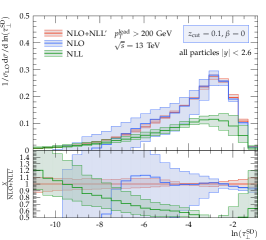
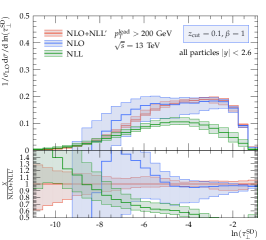
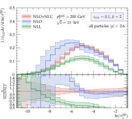
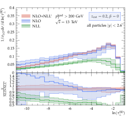
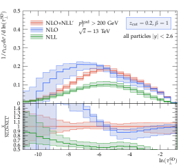
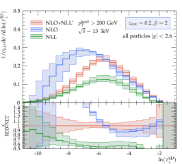
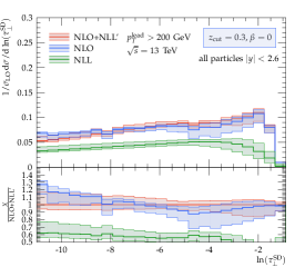
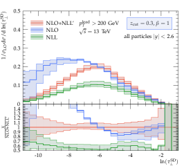
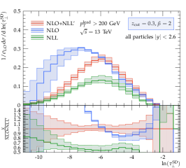
Figure 8: $\text{NLO}+\text{NLL}^{\prime}$ predictions for groomed transverse thrust for $\beta\in\{0,1,2\}$ (columns) and $z_{\text{cut}}\in\{0.1,0.2,0.3\}$ (rows) for the $p_{T,\text{min}}=200\;\text{GeV}$ event selection in comparison to the NLO result and the pure NLL resummation.

In Fig. 8 we present our results for the matched $\text{NLO}+\text{NLL}^{\prime}$ distributions for the $p_{T,\text{min}}=200\;\text{GeV}$ event selection, along with the corresponding NLO and pure NLL predictions. The uncertainty bands shown envelop the $7-$point scale variations for $\mu_{\text{R}}$ and $\mu_{\text{F}}$, i.e. $\{(\tfrac{1}{2}\mu_{\text{R}},\tfrac{1}{2}\mu_{\text{F}})$, $(\tfrac{1}{2}\mu_{\text{R}},\mu_{\text{F}})$, $(\mu_{\text{R}},\tfrac{1}{2}\mu_{\text{F}})$, $(\mu_{\text{R}},\mu_{\text{F}})$, $(\mu_{\text{R}},2\mu_{\text{F}})$, $(2\mu_{\text{R}},\mu_{\text{F}})$, $(2\mu_{\text{R}},2\mu_{\text{F}})\}$, and, for the resummation, separate variations of $\mu_{\text{Q}}$ by factors of $0.5$ and $2$, and the alternative end-point parameter choice $p=2$. The main result, the $\text{NLO}+\text{NLL}^{\prime}$ prediction, is shown in red, with its fixed-order ingredient (NLO) shown in blue, and the resummation contribution (NLL) in green. $\text{NLO}+\text{NLL}^{\prime}$ and NLO are normalised to unity including underflow, cf. Eq. (45). The NLL here is also rescaled by $\sigma_{\text{LO}}=\sigma^{(0)}+\sigma^{(1)}$ instead of just $\sigma^{(0)}$ in order to reflect the limit for the matched distribution when the resummed logarithms dominate. As before we consider $\beta\in\{0,1,2\}$ and $z_{\text{cut}}\in\{0.1,0.2,0.3\}$. In addition the ratio with respect to the $\text{NLO}+\text{NLL}^{\prime}$ result is included.

Grooming an event will reduce the value of transverse thrust, resulting in final states that exhibit a more pencil-like topology. This is evident if we increase the threshold $z_{\text{cut}}$. In consequence the cross section increases for smaller values of $\tau^{\text{SD}}_{\perp}$, including the situation that the event ends up outside the considered plot range. For $\beta>0$ even the peak position is significantly shifted to lower values. When comparing the matched predictions to the pure resummation, we can note that the latter dominates in the soft region, i.e. for $\ln(\tau_{\perp}^{\text{SD}})<-7$ for all $\beta$. However in the ratios it can be seen that there are still significant corrections originating from the $C^{\delta}_{1}$ coefficients and missing NLO logarithms. In particular for $\beta=0$, where the logarithmic enhancement is reduced, effects from the matching can reach up to $40\%$ even in the logarithmic region. In contrast, the fixed-order result dominates in the hard region, i.e. large $\tau_{\perp}^{\text{SD}}$, i.e. for $\ln(\tau_{\perp}^{\text{SD}})>-5$.

The $\text{NLO}+\text{NLL}^{\prime}$ prediction smoothly combines fixed order and resummation, thereby inheriting the strengths of both approaches. It is worthwhile to note that in particular for the case $\beta=0$ the NLO results remain close to the matched prediction even in the logarithmically dominated region. In particular for $z_{\text{cut}}>0.1$ results are found to agree within the NLO uncertainty estimate, however for $z_{\text{cut}}=0.1$ it can be read off from the ratios that the logarithms do still result in significant deviations for $\ln(\tau_{\perp}^{\text{SD}})<-7$. This agreement between $\text{NLO}+\text{NLL}^{\prime}$ and NLO, however, does not hold in general and for $\beta>0$, below $\ln(\tau_{\perp}^{\text{SD}})<-6$, the fixed-order results deviate very strongly from the resummed predictions. This applies in particular for $z_{\text{cut}}>0.1$, while in the $z_{\text{cut}}=0.1$ case the deviation is somewhat smaller and the uncertainties tend to be larger, rendering this statement more ambiguous.

Independent of the considered set of grooming parameters, the $\text{NLO}+\text{NLL}^{\prime}$ results offer a significant reduction of scale-variation uncertainties, when comparing to NLO and pure NLL, respectively. For the fixed order and the NLL these become rather sizeable away from their natural habitat, i.e. in the soft region for the NLO and towards the hard region for the NLL. For the matched predictions scale variations amount to roughly $10\%$ changes in the peak region and for $\beta>0$ somewhat increase towards the hard and soft end of the spectrum where the cross section is significantly reduced.

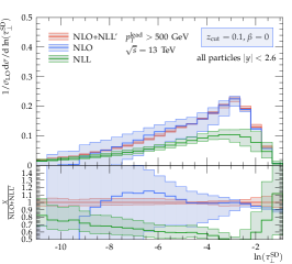
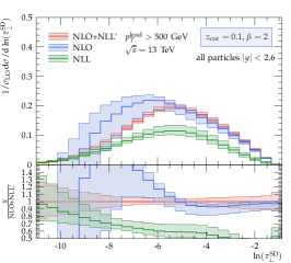
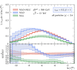
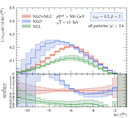
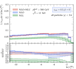
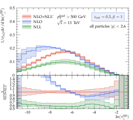
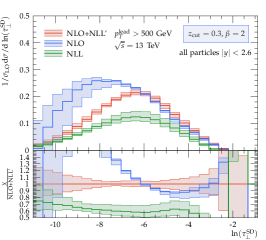
Figure 9: Same as Fig. 8 but for the $p_{T,\text{min}}=500\;\text{GeV}$ event selection.

In Fig. 9 we present corresponding predictions for the $500\;\text{GeV}$ event selection. The results are in fact very similar to the $p_{T,\text{min}}=200\;\text{GeV}$ case. The good agreement of the $\text{NLO}+\text{NLL}^{\prime}$ prediction with the NLO calculation and the pure NLL resummation in the hard and soft region respectively is confirmed. Furthermore, we recover the reduction of scale-variation uncertainties for the matched calculation. In Fig. 19 in Appendix B we compile further results for smaller values of the grooming threshold, namely $z_{\text{cut}}\in\{0.01,0.02,0.05\}$, that will be used in Sec. 4.3 when studying the potential of soft-drop grooming for underlying-event mitigation.

4 Phenomenological studies of soft-drop groomed thrust

In this section we present hadron-level predictions for the soft-drop groomed thrust distribution in proton–proton collisions at $13$ TeV centre-of-mass energy. However, we begin by comparing our $\text{NLO}+\text{NLL}^{\prime}$ accurate predictions to multijet merged parton-level simulations obtained with SHERPA. We then focus on the potential of soft-drop grooming to reduce the impact of the underlying event on the event-shape distribution. To this end we consider particle-level simulations obtained with SHERPA, HERWIG and PYTHIA.

4.1 Monte Carlo simulations – multijet merging, underlying event

To study the event-shape variable at the particle level, and to extract non-perturbative corrections, we compile Monte Carlo predictions based on the SHERPA event generator version 2.2.10 Bothmann:2019yzt . We simulate inclusive dijet production using the MEPS@NLO formalism Hoeche:2012yf ; Hoeche:2012fm , thereby merging the NLO QCD matrix elements for $2-$ and $3-$ and the LO matrix element for the $4-$parton final states obtained from COMIX Gleisberg:2008fv , with virtual corrections obtain from OPENLOOPS Cascioli:2011va , dressed by the SHERPA dipole parton shower Schumann:2007mg . The merging-scale parameter we set to $Q_{\text{cut}}=30\,\text{GeV}$.

To estimate the perturbative uncertainty of the Monte Carlo predictions, we again consider $7-$point variations of the factorisation and renormalisation scales, both in the hard matrix elements and the parton shower, evaluated using on-the-fly reweighting Bothmann:2016nao .

The nominal perturbative scales are defined according to the CKKW-style scale setting prescription Catani:2001cc , cf. Hoeche:2009rj for details. In this procedure the hard-process partons get clustered into a Born-like $2\to 2$ configuration that defines the $2-$jet core process with an associated scale $\mu_{\text{core}}$, that we set to

$$\mu_{\text{core}}=\frac{1}{2}H_{T}\,.$$ (52)

This corresponds to the jet transverse momentum for the reconstructed $2-$jet system and is also used to define the factorisation scale and the shower-starting scale of the core process, i.e.

$$\mu_{\text{F}}=\mu_{\text{Q}}=\mu_{\text{core}}\,.$$ (53)

The effective renormalisation scale, $\mu_{\text{CKKW}}$, of the $n$-parton hard matrix elements corresponds to

$$\alpha_{\text{s}}^{n}(\mu^{2}_{\text{CKKW}})=\alpha_{\text{s}}^{2}(\mu^{2}_{\text{core}})\prod\limits_{i=1}^{n-2}\alpha_{\text{s}}(t_{i})\,,$$ (54)

with $t_{i}$ the reconstructed shower-branching scales.

To account for hadronisation effects we employ SHERPA’s cluster fragmentation model Winter:2003tt . The underlying event simulation uses the SHERPA implementation of the Sjöstrand–Zijl multiple-parton interaction model Sjostrand:1987su . In both models the default set of tuning parameters is used, see Bothmann:2019yzt for details. To contrast and underpin the SHERPA predictions with other theoretical approaches to parton showering and in particular non-perturbative effects Buckley:2011ms , we also compile full particle-level results with HERWIG version 7.2.1 Bellm:2015jjp ; Bellm:2019zci and PYTHIA version 8.240 Sjostrand:2014zea . In both generators we simulate inclusive dijet production at leading order, using the default models and parameters for the underlying event and hadronisation simulations. We also make use of the codes’ default scale-setting that in both cases relates the parton-shower starting scale to the $p_{T}$ of the hard-process jets.

For event selection and analysis we employ the RIVET analysis package Buckley:2010ar .

4.2 Parton-level predictions

In order to further validate our analytic calculations and benchmark the perturbative inputs to our full particle-level Monte Carlo simulations, we compare the SHERPA MEPS@NLO parton-level (PL) predictions against our previously presented resummation results. To be more precise, by PL we here mean terminating the event evolution right after the parton-shower stage, determined by the dipole-shower cutoff $p^{\text{CSS}}_{T,\text{min}}=1\;\text{GeV}$. We then apply our usual event selection to this partonic final state, cf. Sec. 2.2, and include all generated partons with $|y|<2.6$ in the observable evaluation.

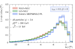
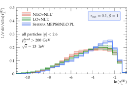
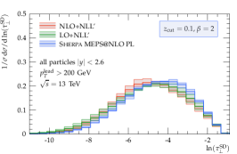
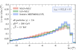
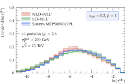
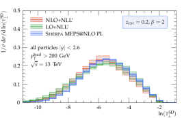
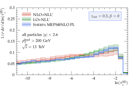
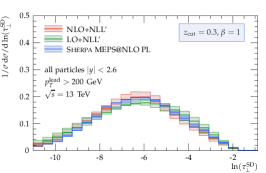
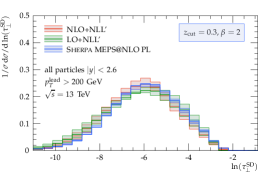
Figure 10: $\text{NLO}+\text{NLL}^{\prime}$ and $\text{LO}+\text{NLL}^{\prime}$ predictions for groomed transverse thrust for $\beta\in\{0,1,2\}$ (columns) and $z_{\text{cut}}\in\{0.1,0.2,0.3\}$ (rows) for the $p_{T,\text{min}}=200\;\text{GeV}$ event selection in comparison to parton-level MEPS@NLO results from SHERPA.

We consider our resummed predictions matched to LO and NLO, i.e. $\text{LO}+\text{NLL}^{\prime}$ and $\text{NLO}+\text{NLL}^{\prime}$, respectively. Complementary to the analytic resummation approach, in parton-shower simulations emissions off the Born process, as well as subsequent emissions thereof, get stochastically generated, thereby accounting for momentum conservation as well as finite recoil effects. In this context, it is important to stress that we also do not attempt to adjust the scale choices and evolution schemes in shower or resummation to particularly match each other which, together with the aforementioned recoil effects, can lead to significant practical differences Hoeche:2017jsi . We here rather aim to compare the resummed results to the exact perturbative input of our phenomenological studies. We hence should not necessarily expect the central values to agree, and rather be prepared to accept incompatibilities as insufficiencies in our error estimates.

In Fig. 10 we compare the three perturbative calculations, with the same grooming parameters as previously, $\beta\in\{0,1,2\}$ and $z_{\text{cut}}\in\{0.1,0.2,0.3\}$, for the $p_{T,\text{min}}=200\;\text{GeV}$ event selection. The MEPS@NLO results, including the scale-uncertainty band, are shown in blue, $\text{NLO}+\text{NLL}^{\prime}$ in red, and $\text{LO}+\text{NLL}^{\prime}$ in green. In Fig. 11 we compile the corresponding results for the $p_{T,\text{min}}=500\;\text{GeV}$ event selection, considering the same set of grooming parameters. We furthermore present predictions for smaller values of the grooming threshold, i.e.  $z_{\text{cut}}\in\{0.01,0.02,0.05\}$ in Fig. 20 in App. B.

For both choices of $p_{T,\text{min}}$, the three predictions yield very similar qualitative results, especially as far as the effect of grooming and the dependence on the parameters $z_{\text{cut}}$ and $\beta$ goes. This holds for the hard end of the spectrum, dominated by the fixed-order components, through the intermediate transition region, as well as for the resummation (multiple emission) dominated small-$\tau_{\perp}^{\text{SD}}$ limit. The matrix-element improved parton-shower simulation fully confirms the observations on the impact of grooming on the distributions shape. By increasing $z_{\text{cut}}$, events are pushed to lower observable values. For $\beta>0$ this even affects the position of the peak of the distributions. We take this agreement as further confirmation of the general effect of our proposed grooming procedure.

For the $200\;\text{GeV}$ selection we observe some quantitative differences, particularly so for $z_{\text{cut}}=0.1$, most significant for the case of $\beta=0$ and $\beta=1$. The MEPS@NLO simulation here predicts a somewhat narrower distribution with a more pronounced peak around the transition point between groomed and ungroomed regions. For the case of ungroomed transverse thrust a similar level of deviation has been observed in previous studies Banfi:2010xy . However, for stronger grooming these differences become smaller and we find in fact a remarkably good agreement, given the theoretical uncertainty. This behaviour is consistent with naive expectations. Soft drop, while not necessarily designed with perturbative ambiguities in mind, after all mainly removes wide-angle radiation that is less constrained.

For the $500\;\text{GeV}$ selection, the results fully confirm our general observations for the $200\;\text{GeV}$ case. The MEPS@NLO and the resummed predictions mostly agree as long as the final state is significantly groomed. Even for the grooming setups where differences were obvious, e.g. $z_{\text{cut}}=0.1$ and $\beta=0,1$, they appear to be reduced in the $500\;\text{GeV}$ case. Again, SHERPA predicts a somewhat narrower distribution than both the $\text{LO}+\text{NLL}^{\prime}$ and $\text{NLO}+\text{NLL}^{\prime}$ for those parameters.

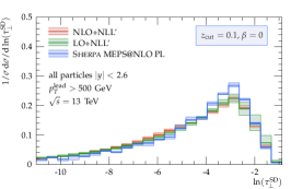
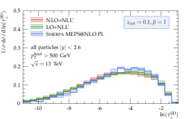
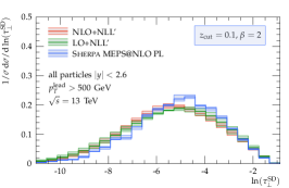
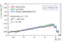
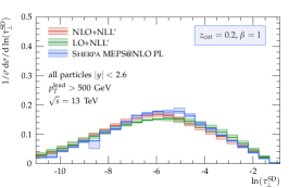
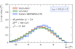
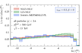
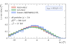
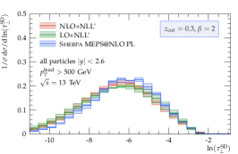
Figure 11: Same as Fig. 10 but for the $p_{T,\text{min}}=500\;\text{GeV}$ event selection.

We conclude from this initial parton-level comparison that the effects of soft-drop grooming are consistently modelled between the SHERPA PL and our resummed calculations, at least for sufficient grooming. To fully interpret the significance of the remaining differences, we should determine and confirm to what level hadronisation and underlying-event corrections are reduced by grooming. We will do exactly that in the following section.

4.3 Underlying event mitigation

After having validated the resummed predictions and compared them to parton-level matrix-element plus parton-shower simulations, the focus shall now shift to studying the impact of non-perturbative corrections on the observable and the potential of soft-drop grooming to reduce their impact. In Fig. 1 we already indicated the typical size of underlying event and hadronisation corrections as they arise for plain transverse thrust. In particular the underlying event results in a significant shift of the distribution towards higher observable values. While the parton-to-hadron fragmentation has a smaller impact for the bulk of the events, it is significant in particular in the low-$\tau_{\perp}$ tail. As the event display in Fig. 2 illustrates, we can expect that soft-drop grooming can be quite efficient in removing the largely uniform underlying-event activity from the final state. This can open the possibility for a more direct reproducibility of experimental measurements by perturbative predictions.

In Fig. 12 we present predictions for groomed transverse thrust for the $p_{T,\text{min}}=200\;\text{GeV}$ event selection obtained with SHERPA taking into account all particles with $|y|\leq y_{\text{max}}$. Results are given after showering the hard process (PL), after including the underlying event (PL+UE), and at full hadron level (HL+UE). For the grooming we again use $\beta\in\{0,1,2\}$, however in order to better illustrate the approach of the ungroomed case, we additionally include a smaller $z_{\text{cut}}$ value and here consider $z_{\text{cut}}\in\{0.05,0.1,0.2,0.3\}$.

For mild grooming with $z_{\text{cut}}=0.05$ and $\beta=0$ underlying-event corrections are indeed of similar size as for the ungroomed case shown in Fig. 1. As we groom harder by enlarging $z_{\text{cut}}$ we observe a more significant reduction in the impact of the underlying event. This is most evident for the case of $\beta=0$ (first column in Fig. 12). For $z_{\text{cut}}=0.1$ the peak is still shifted when including multiple parton interactions, although much less dramatic than for the ungroomed case. Finally, for $z_{\text{cut}}=0.3$ the impact stays below $10\%$. When increasing $\beta$ the effect of the underlying event is further reduced, to the level of at most $20\%$ even for $z_{\text{cut}}=0.1$ for $\ln(\tau_{\perp}^{\text{SD}})>-8$. For $z_{\text{cut}}\geq 0.2$ the underlying-event correction stays well below $10\%$, with the exception of a few seemingly statistical exceptions.

When comparing to the ungroomed case in Fig. 1, hadronisation effects, similar to the $e^{+}e^{-}$ case Baron:2018nfz , are pushed to lower observable values through grooming. This affects predominantly the low-$\tau_{\perp}^{\text{SD}}$ region, where very collimated parton-level jets get spread out. Notably, in the region $\ln(\tau_{\perp}^{\text{SD}})<-8$ the hadronisation corrections change sign when going from $\beta=0$ to $\beta=1,2$. For the latter choices grooming is suppressed for particles with $\Delta R<R_{\text{SD}}$ from the hard jets, accordingly, as in the ungroomed case, hadronisation shifts events towards larger $\tau_{\perp}^{\text{SD}}$. However, even for $\beta=2$ there is a sizeable observable range for which also hadronisation effects are small. Qualitatively, the observed dependence on $\beta$ and $z_{\text{cut}}$ for the transition to the hadronisation dominated regime is well reflected by the estimate derived in Eq. (26) for $a_{l}=b_{l}=1$, also illustrated in Fig. 4. Note, in the Monte-Carlo simulations the parton-to-hadron transition sets in at the parton-shower cut-off scale ${\cal{O}}(1\,\text{GeV})$ already, rather than the Landau pole $\Lambda_{\text{QCD}}$. Furthermore, we are sensitive to the hadronisation of partons originating from the underlying event.

When increasing the scale of the hard dijet-production process by raising $p_{T,\text{min}}$ to $500\;\text{GeV}$, the scale separation of the hard process and the underlying event increases. Accordingly, lower values of $z_{\text{cut}}$ are sufficient to achieve a sizeable reduction of the underlying-event corrections. If the underlying event would be associated with the exact same scales irrespective of the hard-jet $p_{T}$ requirement, we would expect $z_{\text{cut}}$ values scaled by a factor $200/500=0.4$ to yield results in the $p_{T,\text{min}}=500\;\text{GeV}$ case that are comparable to $p_{T,\text{min}}=200\;\text{GeV}$, cf. Eq. (2). We therefore consider $z_{\text{cut}}\in\{0.01,0.02,0.05,0.1\}$ here and present corresponding results in Fig. 13. For $z_{\text{cut}}=0.01$, independent of $\beta$, grooming does not yet significantly reduce the underlying-event contribution. The results for $z_{\text{cut}}=0.02$ are very similar to the findings for $z_{\text{cut}}=0.05$ for $p_{T,\text{min}}=200\;\text{GeV}$ and the reduction observed for the $500\;\text{GeV}$ selection with $z_{\text{cut}}=0.05$ are quite close to those for $z_{\text{cut}}=0.1$ with the lower $p_{T,\text{min}}$. When finally increasing $z_{\text{cut}}$ to $0.1$ we observe agreement between the parton-level predictions with and without the underlying event to better than $10\%$, again with the exception of a few fluctuations due to the limited statistics we could afford for these very demanding simulations. Notably, overall the impact of hadronisation corrections is reduced due to the increased $p_{T,\text{min}}$, and correspondingly $\mu_{\text{R}}$, consistent again with the findings in Sec. 3.3. For $\ln(\tau_{\perp}^{\text{SD}})>-8$ they are in fact rather mild for all values of $z_{\text{cut}}$ and $\beta$ considered here.

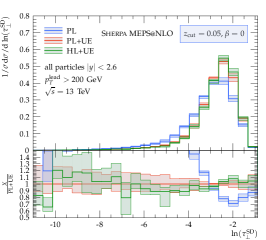
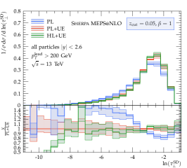
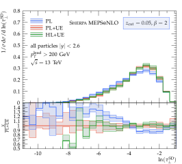
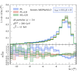
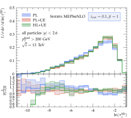
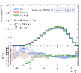
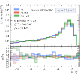
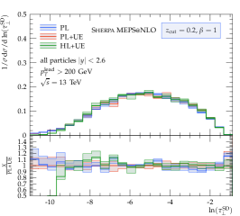
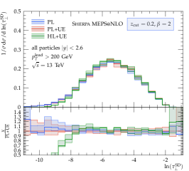
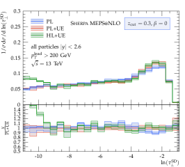
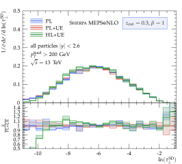
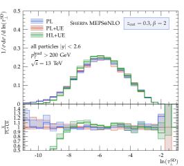
Figure 12: The groomed thrust distributions for $\beta\in\{0,1,2\}$ (columns) and $z_{\text{cut}}\in\{0.05,0.1,0.2,0.3\}$ (rows) for the $p_{T,\text{min}}=200\;\text{GeV}$ event selection. The lower panels show the ratios with respect to the parton-level simulation including the underlying event (PL+UE) prediction.

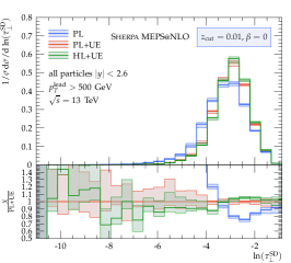
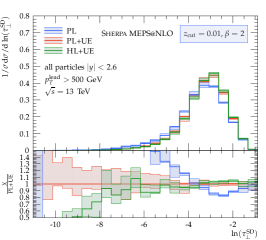
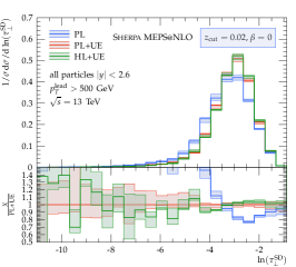
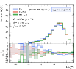
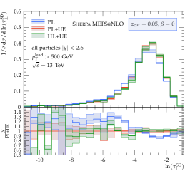
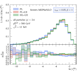
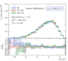
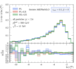
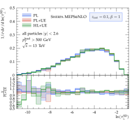
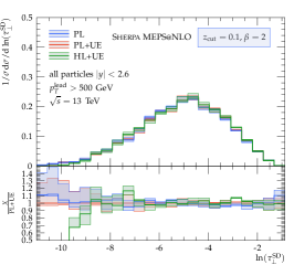
Figure 13: The groomed thrust distributions for $\beta\in\{0,1,2\}$ (columns) and $z_{\text{cut}}\in\{0.01,0.02,0.05,0.1\}$ (rows) for the $p_{T,\text{min}}=500\;\text{GeV}$ event selection. The lower panels show the ratios with respect to the parton-level simulation including the underlying event (PL+UE) prediction.

Track-based observable evaluations

Our current observable definition, based on all final-state particles within the rapidity range $|y|\leq y_{\text{max}}$, requires the use of sophisticated experimental techniques such as particle flow Sirunyan:2017ulk . As a simpler alternative we want to consider the charged final-state particles only, accessible by conventional tracking detectors, for tracks with sufficient transverse momentum in order to be reliably detectable. While these measurement constraints can be imposed on a fully exclusive Monte Carlo simulation, they obscure the comparability with purely perturbative calculations and in addition invoke systematic uncertainties related to the modelling of low-energetic particles in the generators’ hadronisation models. Here we want to study the effect of these constraints on our generator predictions and in particular explore to what extent grooming ameliorates the correspondence with perturbative predictions. To gain statistical power for quantifying the impact of the track-level final-state selections, we produced a high-statistics simplified SHERPA sample setup based on the pure parton shower, i.e. without the inclusion of higher-order matrix elements, denoted SHERPA PS in the following.

In Fig. 14 we compile hadron-level predictions based on SHERPA PS for the $p_{T,\text{min}}=200\;\text{GeV}$ selection for four different inputs to the observable evaluation. We consider the previous default, i.e. all final-state particles without any particle $p_{T}$ requirement, impose an additional track $p_{T}$ cut of $p^{\text{track}}_{T,\text{min}}=500\;\text{MeV}$, and limit to charged particles, with and without the $p^{\text{track}}_{T}$ threshold. As before we consider $\beta\in\{0,1,2\}$ with $z_{\text{cut}}\in\{0.05,0.1,0.2,0.3\}$. We can observe that the impact of calculating the observable on all vs. charged particles only is rather mild, with the exception of regions where the cross section is rather tiny, i.e. towards the kinematic end-point and for very low $\tau_{\perp}^{\text{SD}}$. For the latter region this effect is somewhat more pronounced for $\beta>0$ where grooming is suppressed for objects $\Delta R<R_{\text{SD}}$ away from the hard jets and hadronisation corrections are sizeable. In contrast, the track-quality cut $p_{T,\text{min}}^{\text{track}}$ has a much stronger impact, in particular for $z_{\text{cut}}=0.05$. Here it significantly shifts the distribution, for $\beta=0$ it results in corrections in the peak region of up to $30\%$. Increasing $\beta$ improves the agreement for the bulk of the events. However, when raising $z_{\text{cut}}$ to $0.2$ or $0.3$ all observable definitions agree with the all particles no $p^{\text{track}}_{T,\text{min}}$ staying below $10\%$ for a wide range of $\tau_{\perp}^{\text{SD}}$ values. For events with $p_{T,\text{min}}=500\;\text{GeV}$, corresponding plots are shown in App. B, Fig. 21. The conclusions on the impact of the restriction to charged tracks only and the track-$p_{T}$ cut are in fact very similar. However, as for the underlying-event suppression, the $z_{\text{cut}}$ values needed to reduce the impact of the $p^{\text{track}}_{T,\text{min}}$ criterion scale inversely with the hardness of the hard process and are thus significantly lowered.

In summary, our findings indicate that in particular for heavier grooming resummed predictions could quite directly be compared to experimental data, without significant non-perturbative or track-level corrections.

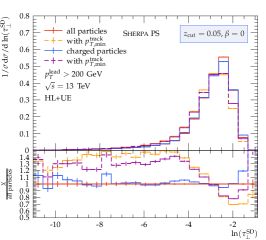
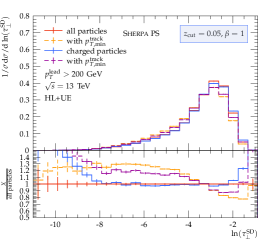
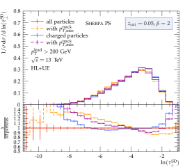
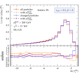
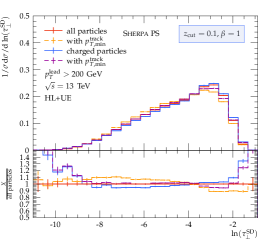
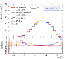
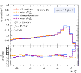
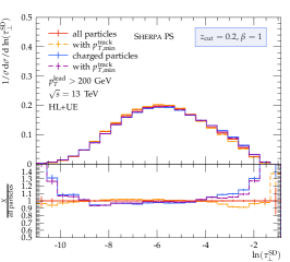
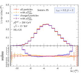
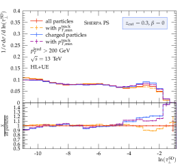
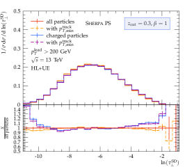
Figure 14: Hadron-level results for groomed thrust for $\beta\in\{0,1,2\}$ (columns) and $z_{\text{cut}}\in\{0.05,0.1,0.2,0.3\}$ (rows) for the $p_{T,\text{min}}=200\;\text{GeV}$ event selection. Shown are predictions from a parton-shower based SHERPA simulation, where the observable gets determined from all or charged final-state particles only. In addition, the effect of a minimal particle transverse-momentum cut of $p^{\text{track}}_{T,\text{min}}=500\;\text{MeV}$ is studied. The lower panels show ratios with respect to the all particles and no track-$p_{T}$ cut prediction.

Generator-level predictions

Based on the SHERPA MEPS@NLO simulations we have demonstrated the potential of soft-drop grooming to reduce the impact of the underlying event on the transverse-thrust distribution. Furthermore, we could show that the effect of constraining the observable evaluation to charged-particle tracks above a minimal $p^{\text{track}}_{T,\text{min}}$ threshold is significantly reduced by soft-drop grooming. This, in fact, allows for a more direct comparison of experimental measurements with perturbative predictions. Furthermore, the tunable sensitivity to the underlying event for different grooming parameters provides means to constrain Monte Carlo generator models for non-perturbative phenomena. Given corresponding measurements, this can be employed in the validation and the tuning of the models and their parameters.

To confirm the viability and robustness of our conclusions and to establish the two use cases, it remains to be studied to what extent our findings are possibly generator specific. To this end, we contrast our hadron-level track-based MEPS@NLO predictions from SHERPA, based on the $2-$ and $3-$jet NLO matrix elements, with track-level results from the HERWIG and PYTHIA generators. For the latter we simulated leading-order dijet production, dressed with parton showers, employing the generators’ default underlying-event and hadronisation models and parameter settings.

In Figs. 15 and 16 we compile the corresponding predictions for the $p_{T,\text{min}}=200\;\text{GeV}$ and $500\;\text{GeV}$ event selections, respectively. We consider the cases $\beta\in\{0,1,2\}$ and $z_{\text{cut}}\in\{0.05,0.1,0.2,0.3\}$ ($p_{T,\text{min}}=200\;\text{GeV}$) and $z_{\text{cut}}\in\{0.01,0.02,0.05,0.1\}$ ($p_{T,\text{min}}=500\;\text{GeV}$). For each set of grooming parameters $z_{\text{cut}}$ and $\beta$ we provide the ratios with respect to the SHERPA hadron-level prediction (first ratio panels), as well as to the corresponding parton-level result of the respective generator, i.e. $\frac{\text{HL+UE}}{\text{PL}}$ for each Monte Carlo (lower ratio panels).

Overall we observe that the three generator predictions agree well for the shape of the track-level thrust distribution for all considered combinations of grooming parameters and both $p_{T,\text{min}}$ selections. In particular in the peak region the differences observed for the hadron-level predictions rarely exceed $10\%$. The results from HERWIG and PYTHIA are very similar and certainly consistent within LO uncertainties. However, the SHERPA MEPS@NLO simulation, using exact NLO matrix elements, produces somewhat harder emission spectra, resulting in more events with larger values of $\tau_{\perp}^{\text{SD}}$. Also in the low-$\tau_{\perp}^{\text{SD}}$ tails the differences can get more significant, in particular for $\beta>0$.

In the lowest panel of the plots we compare for each simulation the fully hadronised prediction with the underlying event included against the corresponding parton-level result. This allows us to extract the non-perturbative corrections for each simulation and provides an estimate for the generator-model dependence. The corrections in fact are very similar for the three simulations. As observed before for the SHERPA simulation, non-perturbative corrections get significantly reduced through grooming also for HERWIG and PYTHIA. For $z_{\text{cut}}\geq 0.2$ for the $200\;\text{GeV}$ selection and $z_{\text{cut}}\geq 0.05$ for $p_{T,\text{min}}=500\;\text{GeV}$ they stay around or below $10\%$ when we consider the region $-7<\ln(\tau_{\perp}^{\text{SD}})<-2$ for all three generators.

The observations in these generator comparisons support the earlier observations. They robustly confirm the finding that soft-drop grooming is very efficient in removing contributions of non-perturbative phenomena from the events’ final state. We further conclude that for the event selections considered here the remaining differences between the various generator predictions are rather mild and mainly affect the tails of the distribution where, however, the event rates are rather small.

This highlights the potential of groomed transverse thrust for precision QCD studies, using fixed- or all-orders predictions. For sufficient grooming the remaining non-perturbative corrections are rather small and seemingly under good control. By lowering the grooming parameters more underlying-event activity can be blended in, providing valuable input to the validation and tuning of phenomenological models in Monte Carlo event generators.

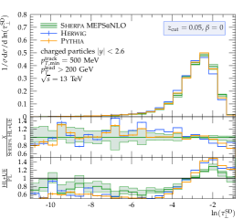
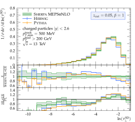
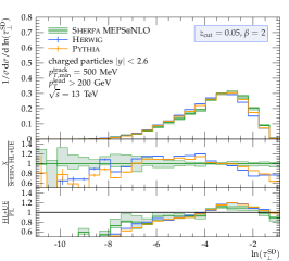
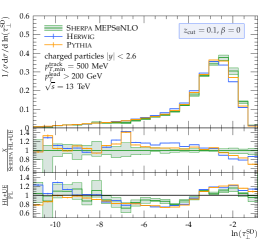
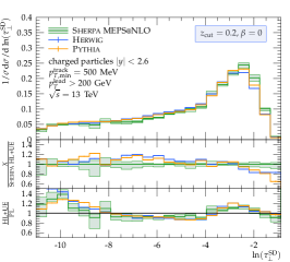
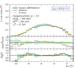
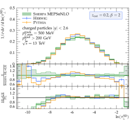
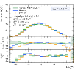
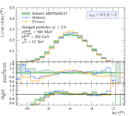
Figure 15: Hadron-level results based on charged-particle tracks with $p^{\text{track}}_{T,\text{min}}>500\;\text{MeV}$ for groomed thrust with $\beta\in\{0,1,2\}$ (columns) and $z_{\text{cut}}\in\{0.05,0.1,0.2,0.3\}$ (rows) for the $p_{T,\text{min}}=200\;\text{GeV}$ event selection. Shown are predictions based on the leading-order dijet production from PYTHIA and HERWIG, as well as the MEPS@NLO result from SHERPA. The two lower panels present the ratios with respect to the SHERPA hadron-level prediction and the generators’ parton-level prediction, respectively.

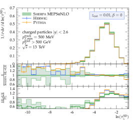
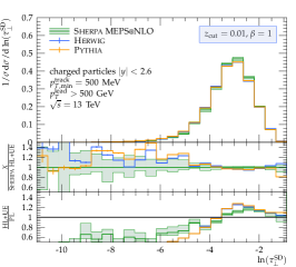
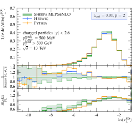
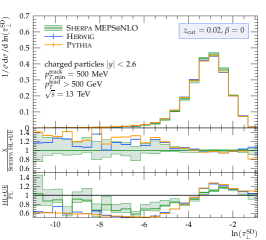
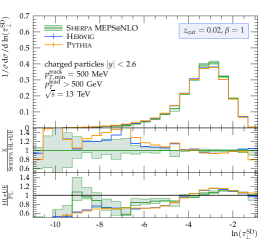
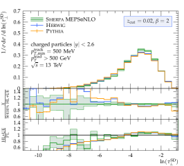
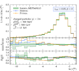
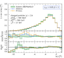
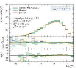
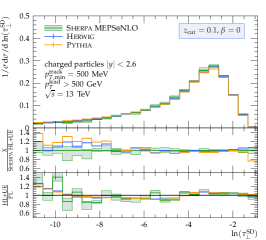
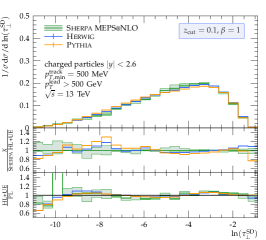
Figure 16: Same as Fig. 15 but for the $p_{T,\text{min}}=500\;\text{GeV}$ event selection and $z_{\text{cut}}\in\{0.01,0.02,0.05,0.1\}$.

5 Conclusions

In this article we considered soft-drop grooming final states of hadronic collisions prior to the evaluation of QCD event-shape variables. This offers great potential to largely remove final-state contributions originating from the underlying event, enabling more direct comparisons of accurate theoretical predictions with experimental data.

To compile first accurate perturbative results, we have extended the well-known CAESAR formalism for the resummation of NLL soft-gluon corrections to groomed event-shape observables in hadronic collisions. We correspondingly generalised the CAESAR implementation in the SHERPA event-generator framework. To take into account exact fixed-order corrections we worked out the matching of the resummation up to NLO accurately split up into flavour channels. With this at hand we provide the means to make $\text{NLO}+\text{NLL}^{\prime}$ accurate predictions for a wide range of hadronic event shapes, with and without grooming.

We focused the first application on groomed transverse thrust in inclusive dijet production at the LHC. This generalisation of the transverse-thrust variable is based on the division of the event final state into two hemispheres that separately get soft-drop groomed. The remaining set of final-state particles, dependent on the chosen set of soft-drop parameters $\beta$ and $z_{\text{cut}}$, then enter the adapted observable evaluation.

We compared our $\text{NLO}+\text{NLL}^{\prime}$ results against state-of-the-art parton-level predictions based on NLO matrix-element improved parton-shower simulations in the MEPS@NLO formalism from the SHERPA event generator. Both methods confirm the feature that grooming shifts the thrust variable to lower values, with larger grooming thresholds $z_{\text{cut}}$ resulting in larger shifts. While for mild grooming we observe notable differences between the two theoretical approaches, the more aggressive the grooming, the better agreement is found.

With the consistency of the two complementary approaches to describe the observable established, we focused on the phenomenology of the groomed thrust variable. In particular we explored the potential of soft-drop grooming to reduce the impact of non-perturbative corrections on the thrust event shape. By comparing Monte-Carlo predictions at parton level with and without the underlying event included, as well as full hadron-level simulations, we found enormous potential of soft-drop grooming to unmask the hard-process final state from non-perturbative contributions. In fact, through sufficient grooming the underlying event can almost entirely be removed, resulting in non-perturbative corrections to the parton-level predictions of less than $10\%$ for a wide range of the observable.

Our initial theoretical considerations have been based on the analysis of all final-state particles, i.e. partons or charged and neutral hadrons, with rapidity $|y|<y_{\text{max}}$. While this can, after grooming, directly be related to resummed predictions, a corresponding experimental analysis would have to employ sophisticated particle-flow techniques. Alternatively, the observable can experimentally be defined on charged-particle tracks above a certain transverse-momentum threshold $p^{\text{track}}_{T,\text{min}}$. Accordingly, we studied the impact of restricting the observable input to charged-tracks with $p^{\text{track}}_{T,\text{min}}=500\;\text{MeV}$. We found that for groomed thrust there remains a close correspondence between the track-based observable and its all-particles variant. We furthermore validated our predictions by comparing to results from HERWIG and PYTHIA, that confirmed our findings with regards to the reduction of non-perturbative corrections for groomed transverse thrust.

In Fig. 17 we summarise our main results by comparing predictions at $\text{NLO}+\text{NLL}^{\prime}$ with MEPS@NLO simulations at parton level, without the underlying event included, and at full hadron level. While the parton-level simulation takes into account all partons, the hadron-level prediction is based on charged-particle tracks with $p^{\text{track}}_{T}>500\;\text{MeV}$. We show representative results for our two dijet event selections. For $p_{T,\text{min}}=200\;\text{GeV}$ we consider the case of rather hard grooming using $z_{\text{cut}}=0.3$ and $\beta=1$. We find that indeed the remaining non-perturbative corrections are significantly reduced over a wide range of $\tau_{\perp}^{\text{SD}}$. Furthermore, the $\text{NLO}+\text{NLL}^{\prime}$ result nicely agrees with the generator predictions. In the $p_{T,\text{min}}=500\;\text{GeV}$ example we instead consider rather mild grooming with $z_{\text{cut}}=0.05$ and $\beta=1$. Even for such low $z_{\text{cut}}$ the non-perturbative corrections are largely reduced, in particular when comparing with the ungroomed case, see Fig. 1. A measurement could hence be sensitive to the differences between perturbative predictions.

Our results indicate that potential future experimental measurements of groomed event shapes offer a great opportunity for precision studies on perturbative QCD, and possibly can differentiate and constrain theoretical approaches based on fixed-order perturbation theory, all-orders resummation, or parton-shower simulations. By varying the hardness of the selected dijet events or the grooming parameters $z_{\text{cut}}$ and $\beta$ the observable offers detailed insights into the transition away from the strict dijet limit. Complementary to this, such variations offer means to tune and constrain the non-perturbative components of Monte Carlo event generators.

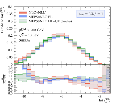
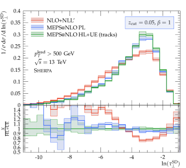
Figure 17: The groomed transverse-thrust distributions for events with a leading-jet transverse momentum $p^{\text{lead}}_{T}>200\;\text{GeV}$, with $z_{\text{cut}}=0.3$ and $\beta=1$ (left) and $p^{\text{lead}}_{T}>500\;\text{GeV}$, with $z_{\text{cut}}=0.05$ and $\beta=1$ (right). Shown are results at $\text{NLO}+\text{NLL}^{\prime}$ accuracy as well as MEPS@NLO predictions obtained with SHERPA at parton level (PL), full hadron level (HL+UE), the latter based on charged tracks with $p_{T}^{\text{track}}>500\;\text{MeV}$. In all cases we only include final-state particles with $|y|<2.6$ in the observable evaluation. The lower panels show the ratios with respect to the HL+UE prediction.

Beyond the transverse-thrust shape considered here, grooming the event final state before evaluating the actual observable can easily be applied to other variables as well. Our derived generalisation of the CAESAR formalism and its implementation in the resummation plugin to the SHERPA framework provides means for largely automated NLL resummation for a wide range of hadronic event shapes. We note that this even applies to observables that measure the deviation from more complex final states than the dijet configuration, with simple modifications such as suitably generalising the notion of splitting of the event into two hemispheres.

Appendix A Logarithmic contributions of $z_{\text{cut}}$

Though we do not perform the resummation of logarithms of $z_{\text{cut}}$ we can outline a method to treat them. First we will elaborate on initial-state radiation, where we follow the same approach as for final-state radiation discussed in Sec. 3.2. In addition, the treatment for soft contributions and PDF ratios will be discussed, neither of which contribute at LL and therefore offer some freedom in their treatment at NLL accuracy.

Initial-State Radiators

For initial-state emissions the same soft-drop condition is used, however the criterion is here taken with respect to the nearest final-state leg in the transverse plane. Accordingly, one can derive

$$p_{T}^{\left(i\right)}=k_{t}^{(l)}\,, p_{T}^{\left(j\right)}=E_{f}\sin\theta\,,$$ (55)

$$\left|\Delta y\right|=\left|\eta^{\left(l\right)}-y_{f}^{\left(l\right)}\right|\,, \left|\Delta\phi\right|=\phi\,,$$ (56)

where $E_{f}$ and $y_{f}^{\left(l\right)}$ denote energy and rapidity of the closest final-state leg to which the emission is clustered. This results in the soft-drop condition:

$$\frac{k_{t}^{(l)}}{E_{f}\sin\theta}>z_{\text{cut}}\left(\frac{\left(\eta^{\left(l\right)}-y_{f}^{\left(l\right)}\right)^{2}+\phi^{2}}{R_{\text{SD}}^{2}}\right)^{\beta/2}\,,$$ (57)

which in the limit of large $\eta^{\left(l\right)}$ results in

$$\frac{k_{t}^{(l)}}{E_{f}\sin\theta}>z_{\text{cut}}\left(\frac{\eta^{\left(l\right)}}{R_{\text{SD}}}\right)^{\beta}\,.$$ (58)

This provides a relation that directly depends on $\eta^{\left(l\right)}$, whereas all other conditions depend on $e^{\eta^{\left(l\right)}}$ only. Accordingly, we are faced with a set of conditions that will not result in simple integration boundaries in $\ln k_{t}^{(l)}$ and $\eta^{(l)}$ simultaneously. We do not calculate the integral associated with it, but note again that from Fig. 18 it is clear that it will not result in any logarithms of $v_{\text{SD}}$ for small enough $v_{\text{SD}}$, hence does not contribute at our target accuracy.

In order to get a better idea of the structure for these contributions an alternative distance measure can be used, namely $\Delta R_{ij}^{2}=2\cosh\left(y_{i}-y_{j}\right)-2\cos\left(\phi_{i}-\phi_{j}\right)$. This definition corresponds to the canonically used relation in the limit of small angular difference. The soft-drop condition then reads

$$\frac{k_{t}^{(l)}}{E_{f}\sin\theta}>z_{\text{cut}}\left(\frac{2\cosh\left(\eta^{\left(l\right)}-y_{f}^{\left(l\right)}\right)-2\cos\phi}{R_{\text{SD}}^{2}}\right)^{\beta/2}\,,$$ (59)

which in the large-$\eta^{\left(l\right)}$ limit instead reduces to

$$\frac{k_{t}^{(l)}}{E_{f}\sin\theta}>z_{\text{cut}}\left(\frac{e^{\eta^{\left(l\right)}}e^{-y_{f}^{\left(l\right)}}}{R_{\text{SD}}^{2}}\right)^{\beta/2}=\frac{2}{\sin\theta}\bar{z}_{\text{cut}}e^{\beta\eta^{\left(l\right)}/2}\,,$$ (60)

where we define $\bar{z}_{\text{cut}}$ such that it absorbs the dependence on $\theta$ and $R_{\text{SD}}$. This condition scales with $\eta^{\left(l\right)}$ in the opposite manner as the final-state contribution, cf. condition (iv) in Sec. 3.2, and results in an increase in grooming when $\beta$ is increased, unless $\eta^{\left(l\right)}\approx y_{f}^{\left(l\right)}$. The result makes sense, since for $\eta^{\left(l\right)}\approx y_{f}^{\left(l\right)}$ the emission is collinear to the final-state leg, but otherwise the value of $\Delta R$ becomes large and results in an enhancement of grooming due to an increase in $\beta$. This can also be seen in the Lund diagram for this condition depicted in Fig. 18.

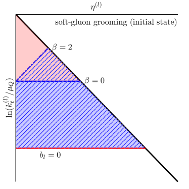
Figure 18: The Lund diagram showing the kinematic constraints for soft drop applied to initial-state emissions. As examples $a_{l}=1$ with $b_{l}=0$ and $\beta=0$ (solid line and area) and $\beta=2$ (dashed line, hatched area) are shown.

The transition point does not work the same as for final-state legs, in fact in general there exist two transition points. Below the first transition there are only logarithms of $z_{\text{cut}}$, in between the two there is a mix of logarithms of $v$ and $z_{\text{cut}}$ and finally above the second transition point there are only logarithms of the observable. Here the two transition points are given by $\bar{z}_{\text{cut}}^{a_{l}},\quad\bar{z}_{\text{cut}}^{\frac{2\left(a_{l}+b_{l}\right)}{2+\beta}}$. Whichever of the two has smaller value defines the first transition point, the other consequently the second one. This does mean that for $2b_{l}=a_{l}\beta$ these two transition points are identical. For transverse thrust the CAESAR parametrisation for initial-state emissions yields $b_{l}=0$, and accordingly, there is only a single transition point when $\beta=0$.

This can be illustrated by the Lund diagram in Fig. 18. As the observable line moves up and the value of the observable increases it will eventually cross the soft-drop line leading to the transition. When $2b_{l}=a_{l}\beta$ the observable and soft-drop bounds are parallel and there will be only a single transition. However, for the $\beta=2$ line we can see that when the observable crosses the left-hand side of the soft-drop bound both conditions contribute to the integral. Once it passes the right-hand side of the soft-drop boundary the observable is the only limit that matters.

In a similar way as was explained for final-state legs in Sec. 3.4 we can shift the transition point by factors and introduce a compensating term, while maintaining NLL accuracy. This means we can choose to shift the $\bar{z}_{\text{cut}}^{a_{l}}$ transition point to be equal to the final-state-leg transition point. However, the second type of transition point cannot be made equal as it depends on a different power of $z_{\text{cut}}$.

Soft Emissions and PDF Contributions

The argument of logarithms from soft wide-angle emissions is directly related to the $k_{t}/\mu_{Q}$ scaling of the lower left-hand corner of a Lund diagram. For both initial- and final-state emissions, in the limit $v\ll z_{\text{cut}}\ll 1$, this is $z_{\text{cut}}$ up to overall factors, which are beyond NLL accuracy. When the distribution transitions for larger values of the observable the scaling changes to the ungroomed case $v^{\frac{1}{a_{l}}}$. This allows us to shift the argument of the logarithms and the transition point for these types of emissions at NLL accuracy to $z_{\text{cut}}^{a_{l}}$. When extending this argument beyond NLL accuracy a separate treatment for initial- and final-state emissions will be needed for the soft function ${\cal{S}}$.

The scale for the ratio of the pdfs also first enters at NLL accuracy. These contributions are linked to the initial-state collinear scaling. This $k_{t}$ scale can be found at the right-hand corner of the Lund diagram, which results in a scaling $z_{\text{cut}}^{\frac{2}{2+\beta}}$. As for the soft function, for larger values of the observable this contribution transitions back to the ungroomed case, which scales as $v^{\frac{1}{a_{l}+b_{l}}}$. This would place the transition point at $z_{\text{cut}}^{\frac{2\left(a_{l}+b_{l}\right)}{2+\beta}}$ similar to the second transition for initial-state emissions.

Appendix B Auxiliary results

Here we collect supplementary material for the validation of the matched resummed predictions, Fig. 19, and parton-level results from SHERPA, Fig. 20, for the $p_{T,\text{min}}$ event selection. In Fig. 21 we present additional results for the generator studies presented in Sec. 4, for the $p_{T,\text{min}}=500\;\text{GeV}$ dijet selection.

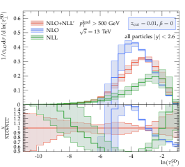
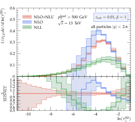
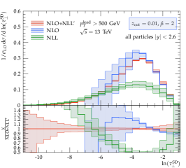
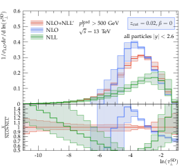
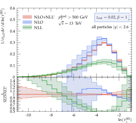
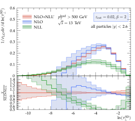
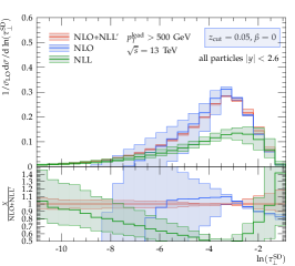
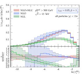
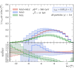
Figure 19: NLL resummed predictions matched to LO and NLO for groomed transverse thrust for $\beta\in\{0,1,2\}$ (columns) and $z_{\text{cut}}\in\{0.01,0.02,0.05\}$ (rows) for the $p_{T,\text{min}}=500\;\text{GeV}$ event selection, cf. Fig. 8 for details.

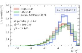
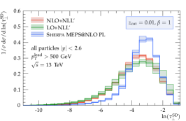
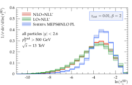
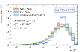
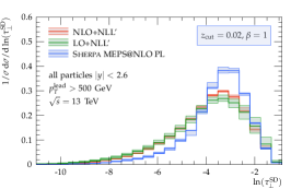
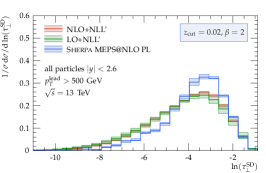
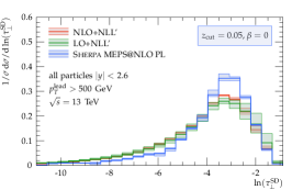
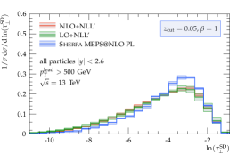
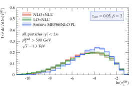
Figure 20: Comparison of NLL resummed results matched to LO and NLO and MEPS@NLO parton-level predictions from SHERPA for groomed transverse thrust for $\beta\in\{0,1,2\}$ (columns) and $z_{\text{cut}}=0.01,0.02,0.05$ (rows) for the $p_{T,\text{min}}=500\;\text{GeV}$ event selection.

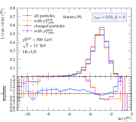
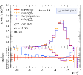
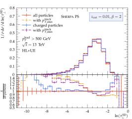
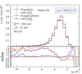
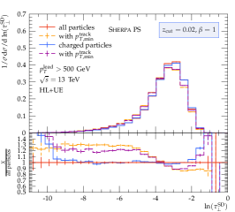
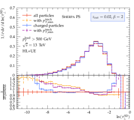
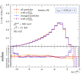
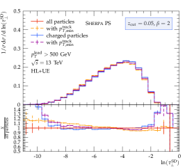
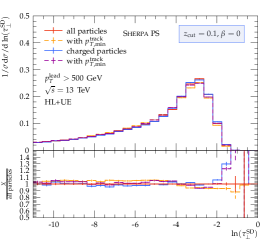
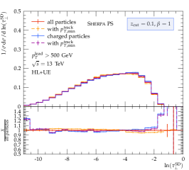
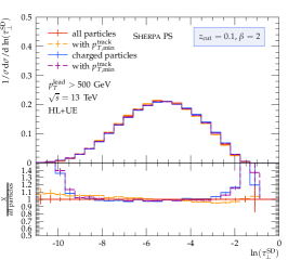
Figure 21: Hadron-level results for groomed thrust for $\beta\in\{0,1,2\}$ (columns) and $z_{\text{cut}}\in\{0.01,0.02,0.05,0.1\}$ (rows) for the $p_{T,\text{min}}=500\;\text{GeV}$ event selection. Shown are predictions from a parton-shower based SHERPA simulation, where the observable gets determined from all or charged final-state particles only. In addition, the effect of a minimal particle transverse-momentum cut of $p^{\text{track}}_{T,\text{min}}=500\;\text{MeV}$ is studied. The lower panels show ratios with respect to the all particles and no track-$p_{T}$ cut prediction.

References

- (1) Y. L. Dokshitzer and B. Webber, Calculation of power corrections to hadronic event shapes, Phys. Lett. B 352 (1995), 451–455, [hep-ph/9504219]
- (2) Y. L. Dokshitzer, G. Marchesini and B. Webber, Dispersive approach to power behaved contributions in QCD hard processes, Nucl. Phys. B 469 (1996), 93–142, [hep-ph/9512336]
- (3) Y. L. Dokshitzer and B. Webber, Power corrections to event shape distributions, Phys. Lett. B 404 (1997), 321–327, [hep-ph/9704298]
- (4) A. Buckley et al., General-purpose event generators for LHC physics, Phys. Rept. 504 (2011), 145–233, [arXiv:1101.2599 [hep-ph]]
- (5) A. Heister et al., The ALEPH collaboration, Studies of QCD at centre-of-mass energies between 91-GeV and 209-GeV, Eur. Phys. J. C 35 (2004), 457–486
- (6) G. Abbiendi et al., The OPAL collaboration, Measurement of event shape distributions and moments in hadrons at 91-GeV - 209-GeV and a determination of alpha(s), Eur. Phys. J. C 40 (2005), 287–316, [hep-ex/0503051]
- (7) J. Abdallah et al., The DELPHI collaboration, A Study of the energy evolution of event shape distributions and their means with the DELPHI detector at LEP, Eur. Phys. J. C 29 (2003), 285–312, [hep-ex/0307048]
- (8) P. Achard et al., The L3 collaboration, Studies of hadronic event structure in annihilation from 30-GeV to 209-GeV with the L3 detector, Phys. Rept. 399 (2004), 71–174, [hep-ex/0406049]
- (9) A. Aktas et al., The H1 collaboration, Measurement of event shape variables in deep-inelastic scattering at HERA, Eur. Phys. J. C 46 (2006), 343–356, [hep-ex/0512014]
- (10) S. Chekanov et al., The ZEUS collaboration, Event shapes in deep inelastic scattering at HERA, Nucl. Phys. B 767 (2007), 1–28, [hep-ex/0604032]
- (11) R. Abbate, M. Fickinger, A. H. Hoang, V. Mateu and I. W. Stewart, Thrust at LL with Power Corrections and a Precision Global Fit for , Phys. Rev. D 83 (2011), 074021, [arXiv:1006.3080 [hep-ph]]
- (12) R. Abbate, M. Fickinger, A. H. Hoang, V. Mateu and I. W. Stewart, Precision Thrust Cumulant Moments at LL, Phys. Rev. D 86 (2012), 094002, [arXiv:1204.5746 [hep-ph]]
- (13) A. H. Hoang, D. W. Kolodrubetz, V. Mateu and I. W. Stewart, -parameter distribution at N3LL’ including power corrections, Phys. Rev. D 91 (2015), no. 9, 094017, [arXiv:1411.6633 [hep-ph]]
- (14) A. Banfi, H. McAslan, P. F. Monni and G. Zanderighi, A general method for the resummation of event-shape distributions in annihilation, JHEP 05 (2015), 102, [arXiv:1412.2126 [hep-ph]]
- (15) Z. Tulipánt, A. Kardos and G. Somogyi, Energy–energy correlation in electron–positron annihilation at NNLL + NNLO accuracy, Eur. Phys. J. C 77 (2017), no. 11, 749, [arXiv:1708.04093 [hep-ph]]
- (16) G. Bell, A. Hornig, C. Lee and J. Talbert, angularity distributions at NNLL′ accuracy, JHEP 01 (2019), 147, [arXiv:1808.07867 [hep-ph]]
- (17) Z.-B. Kang, X. Liu and S. Mantry, 1-jettiness DIS event shape: NNLL+NLO results, Phys. Rev. D 90 (2014), no. 1, 014041, [arXiv:1312.0301 [hep-ph]]
- (18) T. Becher and X. Garcia i Tormo, Factorization and resummation for transverse thrust, JHEP 06 (2015), 071, [arXiv:1502.04136 [hep-ph]]
- (19) T. Becher, X. Garcia i Tormo and J. Piclum, Next-to-next-to-leading logarithmic resummation for transverse thrust, Phys. Rev. D 93 (2016), no. 5, 054038, [arXiv:1512.00022 [hep-ph]], [Erratum: Phys.Rev.D 93, 079905 (2016)]
- (20) L. J. Dixon, M.-X. Luo, V. Shtabovenko, T.-Z. Yang and H. X. Zhu, Analytical Computation of Energy-Energy Correlation at Next-to-Leading Order in QCD, Phys. Rev. Lett. 120 (2018), no. 10, 102001, [arXiv:1801.03219 [hep-ph]]
- (21) A. Gao, H. T. Li, I. Moult and H. X. Zhu, Precision QCD Event Shapes at Hadron Colliders: The Transverse Energy-Energy Correlator in the Back-to-Back Limit, Phys. Rev. Lett. 123 (2019), no. 6, 062001, [arXiv:1901.04497 [hep-ph]]
- (22) L. J. Dixon, I. Moult and H. X. Zhu, Collinear limit of the energy-energy correlator, Phys. Rev. D 100 (2019), no. 1, 014009, [arXiv:1905.01310 [hep-ph]]
- (23) T. Gehrmann, A. Huss, J. Mo and J. Niehues, Second-order QCD corrections to event shape distributions in deep inelastic scattering, Eur. Phys. J. C 79 (2019), no. 12, 1022, [arXiv:1909.02760 [hep-ph]]
- (24) A. Banfi, G. P. Salam and G. Zanderighi, Resummed event shapes at hadron - hadron colliders, JHEP 08 (2004), 062, [hep-ph/0407287]
- (25) A. Banfi, G. P. Salam and G. Zanderighi, Phenomenology of event shapes at hadron colliders, JHEP 06 (2010), 038, [arXiv:1001.4082 [hep-ph]]
- (26) G. Aad et al., The ATLAS collaboration, Measurement of event shapes at large momentum transfer with the ATLAS detector in collisions at TeV, Eur. Phys. J. C 72 (2012), 2211, [arXiv:1206.2135 [hep-ex]]
- (27) V. Khachatryan et al., The CMS collaboration, Study of Hadronic Event-Shape Variables in Multijet Final States in pp Collisions at = 7 TeV, JHEP 10 (2014), 087, [arXiv:1407.2856 [hep-ex]]
- (28) A. M. Sirunyan et al., The CMS collaboration, Event shape variables measured using multijet final states in proton-proton collisions at TeV, JHEP 12 (2018), 117, [arXiv:1811.00588 [hep-ex]]
- (29) G. Aad et al., The ATLAS collaboration, Measurement of hadronic event shapes in high-pT multijet final states at = 13 TeV with the ATLAS detector, JHEP 01 (2021), 188, [arXiv:2007.12600 [hep-ex]]
- (30) A. J. Larkoski, S. Marzani, G. Soyez and J. Thaler, Soft Drop, JHEP 05 (2014), 146, [arXiv:1402.2657 [hep-ph]]
- (31) J. Baron, S. Marzani and V. Theeuwes, Soft-Drop Thrust, JHEP 08 (2018), 105, [arXiv:1803.04719 [hep-ph]], [erratum: JHEP05,056(2019)]
- (32) S. Marzani, D. Reichelt, S. Schumann, G. Soyez and V. Theeuwes, Fitting the Strong Coupling Constant with Soft-Drop Thrust, JHEP 11 (2019), 179, [arXiv:1906.10504 [hep-ph]]
- (33) J. M. Butterworth, A. R. Davison, M. Rubin and G. P. Salam, Jet substructure as a new Higgs search channel at the LHC, Phys. Rev. Lett. 100 (2008), 242001, [arXiv:0802.2470 [hep-ph]]
- (34) S. D. Ellis, C. K. Vermilion and J. R. Walsh, Techniques for improved heavy particle searches with jet substructure, Phys. Rev. D 80 (2009), 051501, [arXiv:0903.5081 [hep-ph]]
- (35) D. Krohn, J. Thaler and L.-T. Wang, Jet Trimming, JHEP 02 (2010), 084, [arXiv:0912.1342 [hep-ph]]
- (36) M. Dasgupta, A. Fregoso, S. Marzani and G. P. Salam, Towards an understanding of jet substructure, JHEP 09 (2013), 029, [arXiv:1307.0007 [hep-ph]]
- (37) F. A. Dreyer, L. Necib, G. Soyez and J. Thaler, Recursive Soft Drop, JHEP 06 (2018), 093, [arXiv:1804.03657 [hep-ph]]
- (38) S. Marzani, G. Soyez and M. Spannowsky, Looking inside jets: an introduction to jet substructure and boosted-object phenomenology, vol. 958, Springer, 2019
- (39) C. Frye, A. J. Larkoski, M. D. Schwartz and K. Yan, Factorization for groomed jet substructure beyond the next-to-leading logarithm, JHEP 07 (2016), 064, [arXiv:1603.09338 [hep-ph]]
- (40) S. Marzani, L. Schunk and G. Soyez, The jet mass distribution after Soft Drop, Eur. Phys. J. C 78 (2018), no. 2, 96, [arXiv:1712.05105 [hep-ph]]
- (41) Z.-B. Kang, K. Lee, X. Liu and F. Ringer, The groomed and ungroomed jet mass distribution for inclusive jet production at the LHC, JHEP 10 (2018), 137, [arXiv:1803.03645 [hep-ph]]
- (42) Z.-B. Kang, K. Lee, X. Liu and F. Ringer, Soft drop groomed jet angularities at the LHC, Phys. Lett. B 793 (2019), 41–47, [arXiv:1811.06983 [hep-ph]]
- (43) G. Bell, R. Rahn and J. Talbert, Two-loop anomalous dimensions of generic dijet soft functions, Nucl. Phys. B 936 (2018), 520–541, [arXiv:1805.12414 [hep-ph]]
- (44) Z.-B. Kang, K. Lee, X. Liu, D. Neill and F. Ringer, The soft drop groomed jet radius at NLL, JHEP 02 (2020), 054, [arXiv:1908.01783 [hep-ph]]
- (45) A. H. Hoang, S. Mantry, A. Pathak and I. W. Stewart, Nonperturbative Corrections to Soft Drop Jet Mass, JHEP 12 (2019), 002, [arXiv:1906.11843 [hep-ph]]
- (46) A. Kardos, A. J. Larkoski and Z. Trócsányi, Two- and three-loop data for the groomed jet mass, Phys. Rev. D 101 (2020), no. 11, 114034, [arXiv:2002.05730 [hep-ph]]
- (47) A. Kardos, A. J. Larkoski and Z. Trócsányi, Groomed jet mass at high precision, Phys. Lett. B 809 (2020), 135704, [arXiv:2002.00942 [hep-ph]]
- (48) D. Anderle, M. Dasgupta, B. K. El-Menoufi, J. Helliwell and M. Guzzi, Groomed jet mass as a direct probe of collinear parton dynamics, Eur. Phys. J. C 80 (2020), no. 9, 827, [arXiv:2007.10355 [hep-ph]]
- (49) A. Banfi, G. P. Salam and G. Zanderighi, Principles of general final-state resummation and automated implementation, JHEP 03 (2005), 073, [hep-ph/0407286]
- (50) E. Gerwick, S. Höche, S. Marzani and S. Schumann, Soft evolution of multi-jet final states, JHEP 02 (2015), 106, [arXiv:1411.7325 [hep-ph]]
- (51) T. Gleisberg, S. Höche, F. Krauss, M. Schönherr, S. Schumann, F. Siegert and J. Winter, Event generation with SHERPA 1.1, JHEP 02 (2009), 007, [arXiv:0811.4622 [hep-ph]]
- (52) E. Bothmann et al., The Sherpa collaboration, Event Generation with Sherpa 2.2, SciPost Phys. 7 (2019), no. 3, 034, [arXiv:1905.09127 [hep-ph]]
- (53) T. Aaltonen et al., The CDF collaboration, Measurement of Event Shapes in Proton-Antiproton Collisions at Center-of-Mass Energy 1.96 TeV, Phys. Rev. D 83 (2011), 112007, [arXiv:1103.5143 [hep-ex]]
- (54) Z. Nagy, Next-to-leading order calculation of three jet observables in hadron hadron collision, Phys. Rev. D 68 (2003), 094002, [hep-ph/0307268]
- (55) A. Banfi, G. P. Salam and G. Zanderighi, Generalized resummation of QCD final state observables, Phys. Lett. B 584 (2004), 298–305, [hep-ph/0304148]
- (56) Y. L. Dokshitzer, G. Leder, S. Moretti and B. Webber, Better jet clustering algorithms, JHEP 08 (1997), 001, [hep-ph/9707323]
- (57) M. Wobisch and T. Wengler, Hadronization corrections to jet cross-sections in deep inelastic scattering, Workshop on Monte Carlo Generators for HERA Physics (Plenary Starting Meeting), 4 1998, pp. 270–279
- (58) A. Kardos, G. Somogyi and Z. Trócsányi, Soft-drop event shapes in electron–positron annihilation at next-to-next-to-leading order accuracy, Phys. Lett. B 786 (2018), 313–318, [arXiv:1807.11472 [hep-ph]]
- (59) E. Farhi, A QCD Test for Jets, Phys. Rev. Lett. 39 (1977), 1587–1588
- (60) A. M. Sirunyan et al., The CMS collaboration, Particle-flow reconstruction and global event description with the CMS detector, JINST 12 (2017), no. 10, P10003, [arXiv:1706.04965 [physics.ins-det]]
- (61) M. Cacciari, G. P. Salam and G. Soyez, The anti- jet clustering algorithm, JHEP 04 (2008), 063, [arXiv:0802.1189 [hep-ph]]
- (62) M. Cacciari, G. P. Salam and G. Soyez, FastJet User Manual, Eur. Phys. J. C72 (2012), 1896, [arXiv:1111.6097 [hep-ph]]
- (63) N. Baberuxki, C. T. Preuss, D. Reichelt and S. Schumann, Resummed predictions for jet-resolution scales in multijet production in e+e- annihilation, JHEP 04 (2020), 112, [arXiv:1912.09396 [hep-ph]]
- (64) G. Luisoni and S. Marzani, QCD resummation for hadronic final states, J. Phys. G 42 (2015), no. 10, 103101, [arXiv:1505.04084 [hep-ph]]
- (65) S. Caletti, O. Fedkevych, S. Marzani, D. Reichelt, S. Schumann, G. Soyez and V. Theeuwes, Jet angularities in Z+jet production at the LHC, JHEP 07 (2021), 076, [arXiv:2104.06920 [hep-ph]]
- (66) S. Catani, L. Trentadue, G. Turnock and B. Webber, Resummation of large logarithms in e+ e- event shape distributions, Nucl. Phys. B 407 (1993), 3–42
- (67) R. W. Jones, M. Ford, G. P. Salam, H. Stenzel and D. Wicke, Theoretical uncertainties on alpha(s) from event shape variables in e+ e- annihilations, JHEP 12 (2003), 007, [hep-ph/0312016]
- (68) A. Banfi, G. P. Salam and G. Zanderighi, Infrared safe definition of jet flavor, Eur. Phys. J. C 47 (2006), 113–124, [hep-ph/0601139]
- (69) T. Gleisberg and S. Höche, Comix, a new matrix element generator, JHEP 12 (2008), 039, [arXiv:0808.3674 [hep-ph]]
- (70) S. Marzani, L. Schunk and G. Soyez, A study of jet mass distributions with grooming, JHEP 07 (2017), 132, [arXiv:1704.02210 [hep-ph]]
- (71) S. Catani and M. Seymour, A General algorithm for calculating jet cross-sections in NLO QCD, Nucl. Phys. B 485 (1997), 291–419, [hep-ph/9605323], [Erratum: Nucl.Phys.B 510, 503–504 (1998)]
- (72) T. Gleisberg and F. Krauss, Automating dipole subtraction for QCD NLO calculations, Eur. Phys. J. C 53 (2008), 501–523, [arXiv:0709.2881 [hep-ph]]
- (73) F. Cascioli, P. Maierhöfer and S. Pozzorini, Scattering Amplitudes with Open Loops, Phys. Rev. Lett. 108 (2012), 111601, [arXiv:1111.5206 [hep-ph]]
- (74) A. Denner, S. Dittmaier and L. Hofer, Collier: a fortran-based Complex One-Loop LIbrary in Extended Regularizations, Comput. Phys. Commun. 212 (2017), 220–238, [arXiv:1604.06792 [hep-ph]]
- (75) R. D. Ball et al., The NNPDF collaboration, Parton distributions for the LHC Run II, JHEP 04 (2015), 040, [arXiv:1410.8849 [hep-ph]]
- (76) S. Höche, F. Krauss, M. Schönherr and F. Siegert, QCD matrix elements + parton showers: The NLO case, JHEP 04 (2013), 027, [arXiv:1207.5030 [hep-ph]]
- (77) S. Höche and M. Schönherr, Uncertainties in next-to-leading order plus parton shower matched simulations of inclusive jet and dijet production, Phys. Rev. D 86 (2012), 094042, [arXiv:1208.2815 [hep-ph]]
- (78) S. Schumann and F. Krauss, A Parton shower algorithm based on Catani-Seymour dipole factorisation, JHEP 03 (2008), 038, [arXiv:0709.1027 [hep-ph]]
- (79) E. Bothmann, M. Schönherr and S. Schumann, Reweighting QCD matrix-element and parton-shower calculations, Eur. Phys. J. C 76 (2016), no. 11, 590, [arXiv:1606.08753 [hep-ph]]
- (80) S. Catani, F. Krauss, R. Kuhn and B. Webber, QCD matrix elements + parton showers, JHEP 11 (2001), 063, [hep-ph/0109231]
- (81) S. Höche, F. Krauss, S. Schumann and F. Siegert, QCD matrix elements and truncated showers, JHEP 05 (2009), 053, [arXiv:0903.1219 [hep-ph]]
- (82) J.-C. Winter, F. Krauss and G. Soff, A Modified cluster hadronization model, Eur. Phys. J. C 36 (2004), 381–395, [hep-ph/0311085]
- (83) T. Sjöstrand and M. van Zijl, A Multiple Interaction Model for the Event Structure in Hadron Collisions, Phys. Rev. D 36 (1987), 2019
- (84) J. Bellm et al., Herwig 7.0/Herwig++ 3.0 release note, Eur. Phys. J. C 76 (2016), no. 4, 196, [arXiv:1512.01178 [hep-ph]]
- (85) J. Bellm et al., Herwig 7.2 release note, Eur. Phys. J. C 80 (2020), no. 5, 452, [arXiv:1912.06509 [hep-ph]]
- (86) T. Sjöstrand, S. Ask, J. R. Christiansen, R. Corke, N. Desai, P. Ilten, S. Mrenna, S. Prestel, C. O. Rasmussen and P. Z. Skands, An introduction to PYTHIA 8.2, Comput. Phys. Commun. 191 (2015), 159–177, [arXiv:1410.3012 [hep-ph]]
- (87) A. Buckley, J. Butterworth, L. Lönnblad, D. Grellscheid, H. Hoeth, J. Monk, H. Schulz and F. Siegert, Rivet user manual, Comput. Phys. Commun. 184 (2013), 2803–2819, [arXiv:1003.0694 [hep-ph]]
- (88) S. Höche, D. Reichelt and F. Siegert, Momentum conservation and unitarity in parton showers and NLL resummation, JHEP 01 (2018), 118, [arXiv:1711.03497 [hep-ph]]