Level Set Percolation in Two-Dimensional Gaussian Free Field

Abstract

The nature of level set percolation in the two-dimension Gaussian Free Field has been an elusive question. Using a loop-model mapping, we show that there is a nontrivial percolation transition, and characterize the critical point. In particular, the correlation length diverges exponentially, and the critical clusters are “logarithmic fractals”, whose area scales with the linear size as $A\sim L^{2}/\sqrt{\ln L}$. The two-point connectivity also decays as the log of the distance. We corroborate our theory by numerical simulations. Possible conformal field theory interpretations are discussed.

Introduction.– Imagine a random landscape being flooded with water. As the water level rises, initially disconnected lakes connect with one another and form eventually an infinite ocean. Does that happen when the flooded area reaches a critical density? If yes, what are the critical properties of the transition? These are the basic questions of the percolation theory of random fields — the relief profile is given by a field $\phi(x)$ and the flooded area $\{x:\phi(x)\leq h\}$ is known as the level set (or excursion set) of height $h$ Efros (1987). Such questions arise naturally in topography and planet science Isichenko (1992); Kalda, J. (2008), but also in transport properties of disordered systems Zallen and Scher (1971); Trugman (1983); Shklovskii and Efros (2013), and have been extensively studied (for recent reviews, see Araújo et al. (2014); Saberi (2015)).

The answer to these questions depends crucially on the statistical properties of the field. If it is short-range correlated, there is a second-order percolation transition Molchanov and Stepanov (1983); Beffara and Gayet (2017); Rivera and Vanneuville (2019): in the thermodynamic limit, infinite clusters (connected components) of the level set never appear below some critical threshold, and always appear above it. The critical point is in the universality class of standard uncorrelated percolation. For long-range correlated fields characterized by a single Hurst roughness exponent $H$, $\left<\phi(x)\phi(y)\right>\sim|x-y|^{2H}$, the situation is richer. When $H<0$, a transition still exists. At criticality, the infinite clusters are fractals, see Fig. 1-(a). Their geometric properties depend on $H$, and have been analytically and numerically characterized Weinrib (1984); Schrenk et al. (2013); Zierenberg et al. (2017); Javerzat et al. (2020a). When $H>0$, there is no sharp transition Schmittbuhl et al. (1993), and the clusters are “compact” objects instead of fractals, see Fig. 1-(c).

A natural question is then what happens at $H=0$, where $\phi$ is log-correlated. This is arguably the most interesting point, especially in two dimensions, as it corresponds to the 2D Gaussian Free Field (GFF). A simple model of elastic interfaces Aarts et al. (2004), its importance in low-dimensional physics Giamarchi (2003), 2D critical phenomena Dotsenko and Fateev (1984) and random geometry Duplantier and Sheffield (2009) cannot be overstated. Despite the enormous amount of studies on the 2D GFF, the percolation of its level sets has been little discussed (by contrast, a number of rigorous results exist for the GFF in $D\geq 3$ dimensions Bricmont et al. (1987); Drewitz et al. (2018) or for the GFF on a transient tree  Abächerli and Sznitman (2018)). There are indeed a few arguments for dismissing this problem as uninteresting. For example, since the correlation length exponent $\nu$ diverges as $H$ approaches zero from below Weinrib (1984), there would be no transition at $H=0$ Isichenko (1992) (see however Schmittbuhl et al. (1993)). Moreover, even if there is a transition, it could be trivial from a geometric point of view Lebowitz and Saleur (1986), since the fractal dimension of the critical clusters approaches $D_{\text{f}}=2$ in the same limit Zierenberg et al. (2017); Javerzat et al. (2020a); Schoug et al. (2019).

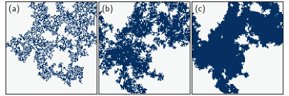
Figure 1: Level set percolation in random fields with different roughness exponents. (a) When $H=-1<0$, there is a percolation transition, with fractal clusters appearing at criticality. (b) When $H=0$ (2D GFF), the critical clusters are logarithmic fractals. (c) When $H=\frac{1}{2}>0$, there is no sharp transition, and the clusters are not fractal.

However, these conclusions can be challenged by looking at some large level set clusters of the 2D GFF, shown in Fig. 1 (b). They are apparently distinct from their $H>0$ as well as $H<0$ counterparts. Numerical simulations also indicate a sharp transition at a critical density $1/2$ in the thermodynamic limit, see Fig. 2. Could the above arguments have missed something subtle?

In this Letter, we revisit the problem of level set percolation in the 2D GFF. By an analytical argument based on the loop-model reconstruction of the 2D GFF, we show that its level set percolation is a nontrivial critical phenomenon, characterized by an exponentially diverging correlation length. At criticality, we find that the area of the large clusters with linear size $L$ scales as

$$A\sim\frac{L^{2}}{\sqrt{\ln L}}\,.$$ (1)

So, the clusters have the same fractal dimension $2$ as compact Euclidean forms, but differ from them by a log correction. Such geometric objects have been named “log fractals” Mandelbrot (1982); Falconer (2004); Indekeu and Fleerackers (1998). A remarkable example of log fractals is the set of points visited by a random walk on a 2D lattice, which satisfies $A\sim L^{2}/\ln L$ Dvoretzky and Erdős (1951); Kundu et al. (2013). We will also show that the probability that two points $x,y$ belong to the same level cluster has a peculiar log decay:

$$P_{2}(x,y)\approx C-\frac{1}{\pi}\frac{\ln\left|x-y\right|}{\ln L}\,,$$ (2)

where $C$ is an unknown constant and $L$ is the system size.

Figure 2: Percolation threshold of 2D GFF level sets on square lattices of size $L\times L$. Main: The existence probability of a percolating cluster $P_{L}(f)$, where $f=(\text{level set area})/L^{2}$ is the level set’s mean density. Inset: Finite-size scaling collapse according to the correlation length prediction (16), identifying $\xi=L$. The critical value $f_{c}=1/2$ regardless of lattice details. All numerics in this paper are done with real-valued 2D GFFs on periodic square lattices, generated by the standard Fourier filter method Prakash et al. (1992); sup .

GFF by loop model.– The 2D GFF can be defined by the action

$$\mathcal{S}[\phi]=\frac{g}{4\pi}\int\left[\nabla\phi(x)\right]^{2}\mathrm{d}^{2}x$$ (3)

(the probability of $\phi$ is proportional to $e^{-\mathcal{S}[\phi]}$) where $g$ is the coupling constant, which also determines the log correlation of $\phi$,

$$\left<\phi(x)\phi(y)\right>=-\frac{1}{g}\ln\left|x-y\right|\,.$$ (4)

Its short-distance divergences need to be regularized in some way. Here, we shall do this by using the $\mathrm{O}(n=2)$ loop model on the honeycomb lattice Cardy and Ziff (2003), as reviewed below. We expect the critical properties of the level set percolation do not depend on the choice of regularization.

The $\mathrm{O}(n)$ loop models can be defined by a partition function which sums over all configurations $\mathcal{C}$ of disjoint loops on the lattice, see Fig. 3-(a):

$$\mathcal{Z}=\sum_{\mathcal{C}}n^{N_{\mathcal{C}}}K^{L_{\mathcal{C}}}\,,$$ (5)

where $n$ and $K$ are fugacities associated with the number of loops $N_{\mathcal{C}}$ and the their length $L_{\mathcal{C}}$, respectively. When $n=2$, for any $K\geq K_{c}=1/\sqrt{2}$, the model is critical and described by a conformal field theory (CFT) with central charge $c=1$, see e.g. Estienne and Ikhlef (2015); Jacobsen (2012). Given a loop configuration, we can assign a random orientation to each loop, and define a height function $\phi$ on the lattice faces such that the loops are its oriented contour lines, with a step $\pm\pi$ across each loop. Assuming the Dirichlet boundary condition for $\phi$ in a simply connected domain, that is, using $\phi|_{\text{boundary}}=0$ as the starting point, the height configurations are in one-to-one correspondence with oriented loop configurations . It is well known that the scaling limit of the height function is a 2D GFF with a coupling constant satisfying

$$n=-2\cos(\pi g)\stackrel{{\scriptstyle n=2}}{{\Rightarrow}}g=1\,.$$ (6)

The above mapping is the first step to the Coulomb gas approach, that has been applied for studying certain random sets of the GFF, notably the loops and the regions between them Duplantier and Saleur (1989) (see Werner and Powell (2020) and references therein for rigorous works). However, the Coulomb gas approach fails to capture the level cluster, but we can still use the mapping to study them.

Application to percolation.– Now that we have a 2D GFF $\phi$ regularized on simply-connected domain with Dirichlet boundary condition, let us consider the level set $\{\phi\leq h\}$ for $h>0$. The infinite cluster is defined as the set of points that are connected to boundary by a path in the level set. Note that the gasket, i.e., the region not encircled by any loop, is a subset of the infinite cluster. Now, let $z$ be inside a hexagon, the following probability

$$P_{\infty}(z,h):=\mathrm{Prob}(z\in\text{the infinite cluster})$$ (7)

is the order parameter in percolation theory. It encodes in particular the basic critical exponents.

A little thought shows that this has much to do with the number $d_{z}$ of loops that encircle $z$. Indeed, consider a path from the boundary to $z$ that only crosses the $d_{z}$ loops encircling $z$, see Fig. 3-(b). $z$ is in the infinite cluster if and only if $\phi\leq h$ along this path. By the loop-model construction, the values of $\phi$ along the path, denoted $\{Z_{j}\}_{j=0}^{d_{z}}$, form an unbiased 1D random walk with steps $\pm\pi$

$$Z_{0}=0\,,\,Z_{j}-Z_{j-1}=\pm\pi\,,\,j=1,\dots,d_{z}\,.$$ (8)

A classical result states that this random walk never goes above $h$ with the following probability (see e.g. Wiese et al. (2011)):

$$\mathrm{Prob}(\forall j\leq d_{z},Z_{j}\leq h)\approx\mathrm{erf}\left(\frac{h}{\pi\sqrt{2d_{z}}}\right)\theta(h)\,,$$ (9)

provided $d_{z}\gg 1$. Since $\mathrm{Prob}(\forall j\leq d_{z},Z_{j}\leq h)$ is the probability (7) conditioned on the random number $d_{z}$, the order parameter can be obtained by averaging over $d_{z}$. In the scaling limit, this can be done by simply treating $d_{z}$ as deterministic and replacing it by its mean value:

$$P_{\infty}(z,h)\approx\mathrm{Prob}(\forall j\leq\left<d_{z}\right>,Z_{j}\leq h)\,.$$ (10)

To justify this, observe first that the mean value of $d_{z}$ is related to the variance of $\phi(z)$:

$$\left<d_{z}\right>=\frac{1}{\pi^{2}}\,\left<\phi(z)^{2}\right>\approx\frac{1}{\pi^{2}}\ln L\,,$$ (11)

where $L$ is the lattice size, for any $z$ far from the boundary (in lattice units). Meanwhile, the fluctuations of $d_{z}$ are of order $\sqrt{\ln L}$ Kesten and Zhang (1997); Schramm et al. (2009), so can indeed be neglected compared to $\left<d_{z}\right>$ sup as $L\to\infty$. Combining (9) to (11), we have

$$P_{\infty}(z,h)\approx\mathrm{erf}\left(\frac{h}{\sqrt{2\ln L}}\right)\approx\frac{h}{\sqrt{\frac{\pi}{2}\ln L}}\,,$$ (12)

where we linearized $\mathrm{erf}(x)$ around $x=0$. Therefore (12) is valid in the scaling limit $L\to\infty$ with fixed $h>0$ and $z$ far from the boundary.

With the result (12) at hand, we can derive most of the claims in the Introduction. Eq. (1) is immediately obtained by summing (12) over the $\sim L^{2}$ lattice points. The nature of the log fractal is manifest in the fact that the probability of a point belonging to it decays logarithmically in $L$, as opposed to algebraically in a usual fractal. The order parameter exponent $\beta$ can be also obtained. Introducing the mean density of the level set,

$$f =\mathrm{Prob}(\phi(z)\leq h)=\int_{-\infty}^{h}e^{-{x^{2}}/(2{\ln L})}\frac{\mathrm{d}x}{\sqrt{2\pi\ln L}}$$

$$\approx\frac{1}{2}+\frac{h}{\sqrt{2\pi\ln L}}$$ (13)

for $h\sim\mathcal{O}(1)$ and $L\to\infty$, $\beta$ is defined by the non-analyticity of $P_{\infty}$:

$$P_{\infty}(f>f_{c})\sim(f-f_{c})^{\beta}\,.$$ (14)

Comparing (12), (13), and (14), we have

$$\beta=1\,,$$ (15)

as well as $f_{c}=1/2$; the latter is observed numerically, see Fig. 2. Finally, comparing $P_{\infty}\sim(f-f_{c})^{1}$ and $P_{\infty}\sim 1/\sqrt{\ln L}$ (12), and assuming that close to the critical point, the correlation length $\xi\sim L$, we find that $\xi$ diverges exponentially near criticality such that

$$|f-f_{c}|\sim\frac{1}{\sqrt{\ln\xi}}\,.$$ (16)

This is in nice agreement with numerical simulations shown in Fig. 2, and explains why the transition sharpens extremely slowly as the system size increases. We note that in the thermodynamic limit, any value $h=\mathcal{O}(1)$ is critical, even if $h\leq 0$ (the restriction $h>0$ above has to do with the specific setup of the Dirichlet boundary condition and the definition of the infinite cluster).

It is useful to contextualize the above results as the limit of level set percolation with $H<0$. It was shown by an extended Harris criterion Weinrib (1984) that when $H\in(-3/4,0)$, the correlation length exponent $\nu(H)=-1/H$. The level cluster’s fractal dimension $D_{\text{f}}(H)$ is not known exactly, yet numerics Zierenberg et al. (2017); Javerzat et al. (2020a) suggest that $D_{\text{f}}(H\to 0)=2$. Our analysis explains these limiting behaviors: $\nu({H=0})=\infty$ because the correlation length diverges faster than any power law, and $D_{\text{f}}(0)=2$ because we have a log fractal. Moreover, assuming that $\beta$ is continuous at $H=0_{-}$, we have by hyperscaling

$$D_{\text{f}}(H)=2-\frac{\beta(H)}{\nu(H)}=2+H+\mathcal{O}(H^{2})\,,\,H<0\,.$$ (17)

We also remark that the boundaries of the level cluster, i.e., the loops, are described by the Schramm-Loewner evolution, SLE_κ=4 Schramm and Sheffield (2009, 2013), and have a fractal dimension $3/2$ . This fractal dimension corresponds to a primary operator in the CFT of the $\mathrm{O}(2)$ loop model. The same CFT also describes the interior regions between loops, which have a fractal dimension $15/8$. However, the level cluster does not seem to be described by any known CFT. It is a very different object, depending on the “random topology”, rather than the random geometry, of the loops.

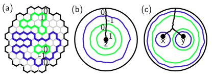
Figure 3: (a) A loop model configuration on a honeycomb lattice and the associated height field $\phi$ (heights are in unit of $\pi$). The color of a loop (blue/green) determines the increment of $\phi$ across it; $\phi$ is constant in regions between loops. (b) A point $z$ encircled by $d_{z}=4$ loops, and a path from the boundary to $z$ (without crossing other loops that are not drawn). The field along the paths gives a random walk realization $\{Z_{j}\}=0,-1,0,1$. (c) Two points $x$ and $y$ satisfying $q=2$, $d_{x}=3$, $d_{y}=4$, connected to the boundary by a branching path. The random walk realization $\{X_{j}\}=0,-1,0,-1$ and $\{Y_{j}\}=0,-1,0,1,0$ share the first $q$ steps.

Two-point connectivity.– To further illustrate this point, let us consider another standard observable in percolation: the two-point connectivity $P_{2}(x,y)$ at criticality, the probability that $x$ and $y$ are in the same connected component of the level set $\{\phi\leq h\}$, for any fixed $h=\mathcal{O}(1)$. This observable has been shown recently to probe very subtle universal properties of critical clusters Javerzat et al. (2020a, b). Similarly to $P_{\infty}$ above, $P_{2}(x,y)$ can be calculated by conditioning on the loop configurations. More precisely, we condition on $d_{x},d_{y}$, and also $q$, the number of loops that encircle both points, see Fig. 3-(c). The random walks $X_{0},\dots,X_{d_{x}}$, and $Y_{0},\dots,Y_{d_{y}}$ that record the field value evolution from the boundary to $x$ and $y$ have the same first $q$ steps:

$$X_{j}=Y_{j}\,,\,j=0,\dots,q\,,$$ (18)

while the remaining $d_{x}-q$ and $d_{y}-q$ steps are independent (we have a branching random walk). Then, it is not hard to see that the two-point connectivity conditioned on $d_{x},d_{y}$ and $q$ is the probability that the “forked” part of the branching random walk never goes above $h$:

$$P_{2}(d_{x},d_{y},q)=\mathrm{Prob}(\forall i,j\geq q,X_{i}\leq h,Y_{j}\leq h)\,.$$ (19)

The common part ($<q$) is not further constrained since we do not require $x,y$ to belong to the infinite cluster. Similarly to (9) above, we have

$$P_{2}(d_{x},d_{y},q)$$

$$\approx \int_{0}^{\infty}\mathrm{erf}\left(\frac{u\sqrt{q}+h}{\sqrt{2s_{x}}}\right)\mathrm{erf}\left(\frac{u\sqrt{q}+h}{\sqrt{2s_{y}}}\right)\frac{e^{-\frac{u^{2}}{2}}\mathrm{d}u}{\sqrt{2\pi}}$$ (20)

as long as $s_{x}:=d_{x}-q,s_{y}:=d_{y}-q$ and $q$ are all much larger than $1$. In that limit $h=\mathcal{O}(1)$ can be also neglected. Like $d_{x}$ and $d_{y}$, the mean value of $q$ is fixed by the covariance of the GFF:

$$\left<q\right>=\frac{1}{\pi^{2}}\left<\phi(x)\phi(y)\right>\approx\frac{1}{\pi^{2}}\ln\frac{L}{|x-y|}\,,$$ (21)

and $q$ also becomes deterministic when $L/|x-y|\gg 1$ sup . As a result, we find

$$P_{2}(x,y)\approx\int_{0}^{\infty}\mathrm{erf}\left(\frac{u\sqrt{\ln\frac{L}{|x-y|}}}{\sqrt{2\ln|x-y|}}\right)^{2}\frac{e^{-\frac{u^{2}}{2}}\mathrm{d}u}{\sqrt{2\pi}}\,,$$ (22)

valid in the scaling limit: $1\ll|x-y|\ll L$, with $x,y$ far from the boundary. In the regime where $|x-y|\gg\sqrt{L}$, the error functions can be linearized, and (22) simplifies to (2) in the Introduction, with the offset predicted as $C=1/\pi$.

We now test (2) numerically, see Fig. 4. The results confirm nicely the $\ln|x-y|/(\pi\ln L)$ dependence on the distance predicted in (2), including the exact prefactor and throughout the scaling regime. On the other hand, the offset $C$ does not agree with the analytical prediction. The reason of this is two-fold. First, we recall that Eq. (22) is derived on a simply connected domain with Dirichlet boundary condition, while the numerics is performed on a torus (see caption of Fig. 2). Moreover, we are a priori far from the thermodynamic limit. Indeed, our analytical argument relied on a large average number of encircling loops. Yet, according to (11), there are in average $0.8$ loops encircling a point in a lattice of $L=2048$ (even on an Avogadro-scale lattice with $L=10^{10}$, there would be $2.3$ loops in average). The offset is affected by the different infrared regularization, and the abundance of realizations with few loops. In contrast, the $\ln|x-y|/(\pi\ln L)$ dependence appears to be remarkably robust. Therefore, we propose (2), with an unknown offset $C$, as a general prediction of two-point connectivity.

The log in (2) can be explained by a rather simple argument. Indeed, for $H<0$, the level clusters are standard fractals, with the two-point connectivity decaying as a power law $P_{2}(H)\sim|x-y|^{2(D_{\text{f}}(H)-2)}$ Kapitulnik et al. (1984). By (17), $P_{2}(H)\sim 1+2H\ln|x-y|$ for $H$ close to $0$ and $\ln|x-y|\ll 1/(-H)$. Now, in this regime, a field with $H<0$ is indistinguishable from a 2D GFF in a system of size $L$ such that $\ln L=1/(-H)$ sup . Therefore we can rewrite $P_{2}(H)\sim 1-\ln|x-y|/\ln L$, recovering the form of (2).

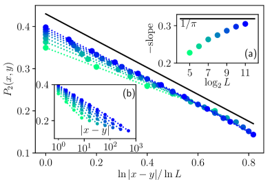
Figure 4: Testing the two-point connectivity prediction (2) with $h=0$ level sets of the 2D GFF on periodic square lattices of size $L\times L$. Main. The averaged two-point connectivity $P_{2}(x,y)$ as a function of $\ln|x-y|/\ln L$. The dots are numerical measure with $L=32,64,\dots,2048$; see inset (a) for color code. The solid line represents the prediction (2) (with the exact slope $1/\pi$ and arbitrarily adjusted offset $C$). Inset (a) The slope as a function of system size, obtained by a global linear fit of each curve. A convergence to the prediction $1/\pi$ as $L\to\infty$ is observed. Inset (b) The raw data. Plotting $P_{2}$ against $|x-y|$ as usual, we observe no collapse. The dotted lines are a guide to the eye.

Conclusion.– We showed that the level sets of the 2D Gaussian Free Field have a nontrivial percolation transition, and outlined a theory of the critical point. In particular, the critical level clusters are found to be log fractals, whose connectivity properties are determined by the random topology of the contour lines. The analysis presented above can be extended to any $n$-point connectivity, which is mapped to a branching random walk. The emergence of such a hierarchical structure in the 2D GFF is not at all new. For instance, it is crucial in the problem of extreme value statistics of the 2D GFF, also known as log-correlated random energy models, or multiplicative chaos Chamon et al. (1996); Carpentier and Le Doussal (2001); Fyodorov and Bouchaud (2008); Rhodes and Vargas (2014); Madaule et al. (2016). The latter problem admits, nevertheless, a conformal field theory description Cao et al. (2017, 2018); Remy (2020). Whether the same can be said of the level clusters of the 2D GFF seems to be an interesting question. We remark that the level clusters for $H<0$ seem to be described by a new CFT, some features of which have been numerically studied Javerzat et al. (2020a). As discussed above, the logs that appear in (2) can be obtained from certain correlators in the $H<0$ CFT, which do not involve an indecomposable representation of the conformal symmetry Santachiara and Viti (2014); Nivesvivat and Ribault (2020), or a continuous spectrum Ribault (2014). Whether such structures exist in the putative $H=0$ CFT remains to be seen.

We thank Sebastian Grijalva, Nina Javerzat and Alberto Rosso for collaborations on related questions, and Malte Henkel, Pierre Le Doussal, Satya Majumdar, Sylvain Ribault and Hugo Vanneuville for helpful discussions.

.1 Numerical Methods

Gaussian Free Fields. The numerical tests are all performed on a square lattice of size $L\times L$, with periodic boundary conditions on both directions, $x\equiv x+L$, $y\equiv y+L$. The 2D GFF can be numerically generated by the standard Fourier filter method:

$$\phi(x,y):=\mathrm{Re}\left({\sum_{\begin{subarray}{c}p,q=1,\dots,L\\ (p,q)\neq(0,0)\end{subarray}}}e^{\frac{2\pi}{L}\mathbf{i}(qx+py)}\left(\sin\left(\frac{q\pi}{L}\right)^{2}+\sin\left(\frac{p\pi}{L}\right)^{2}\right)^{-\frac{1+H}{2}}\mathcal{N}_{p,q}\right)\,,\,x,y=1,\dots,L\,.$$ (23)

Here, $H=0$ gives us the 2D GFF, while $H\neq 0$ corresponds to fractional GFF with a Hurst exponent $H$. $\mathcal{N}_{p,q}$ are independent random complex variables whose real and imaginary pars are independent and have standard Gaussian distribution, with zero mean and variance equal to $1$. The discrete Fourier transform is efficiently performed by the Fast Fourier Transform algorithm.

Percolation clusters. For a given field realization $\phi(x,y)$ and a level $h$, we consider a non-directed graph whose vertex set is the level set, $V=\{(x,y):\phi(x,y)\leq h\}$. Two vertices $(x,y)$ and $(x^{\prime},y^{\prime})$ are connected if they are nearest neighbors: $(x^{\prime},y^{\prime})=(x\pm 1,y)$ or $(x^{\prime},y^{\prime})=(x,y\pm 1)$. The level set clusters are defined the connected components of this graph.

The above procedure defines the site percolation on a square lattice. We can also consider the bond percolation by adding an edge between $(x,y)$ and $(x^{\prime},y^{\prime})$, whenever $(x^{\prime},y^{\prime})\in\{(x+(-1)^{x+y},y+(-1)^{x+y}),(x-(-1)^{x+y},y-(-1)^{x+y})\}$ (we assume $L$ is even). The idea is that we view the lattice $\{(x,y)\}$ as that of the middle point of the edges of another square lattice.

For the figures of this paper, we used the bond percolation. We checked that our results still hold with site percolation.

Method for Figure 1. We take a fixed realization of the complex Gaussians $\{\mathcal{N}_{p,q}\}_{p,q=1}^{L}$ to generate three fraction GFFs with $H=-1,0,1/2$, respectively. Then we plot the largest level set cluster with $h=0$.

Method for Figure 2. For each $L$, we generate $S=10^{3}$ realizations. For each realization $\phi_{i}$, we look for the percolation threshold

$$h_{i}:=\sup\{h:\text{The level set}\{(x,y):\phi_{i}(x,y)\leq h\}\text{ has no percolating cluster}\}$$ (24)

by a bisection search (the notion of percolating cluster is defined below). Then the threshold fraction is

$$f_{i}:=|\{(x,y):\phi_{i}(x,y)\leq h_{i}\}|/L^{2}\,.$$ (25)

Then, we plot $P_{L}(f)$, the empirical cumulative distribution of $\{f_{i},i=1,\dots,S\}$:

$$P_{L}(f):=|\{i=1,\dots,S:f_{i}\leq f\}|/S\,.$$ (26)

The percolating cluster is defined as follows. We eliminate the edges that connect a vertex with $y=1$ to one with $y=L$ (that is, we cut the torus into a cylinder). Then a percolating cluster is one that intersects both boundaries $\{(x,y):y=1\}$ and $\{(x,y):y=L\}$.

Method for Figure 4. For each $L\in\{2^{5},2^{6},\dots,2^{11}\}$, we generated $10^{3}$ GFF realizations, and determine the level set clusters with $h=0$. We calculate whether $(x,y)$ and $(x+r,y)$ are in the same level set cluster, for $r=1,2,4,8,\dots,L/4$ and all $(x,y)$ in the lattice. Averaging over $(x,y)$ and realizations gives us a good estimate of $P_{2}(r)$.

.2 Remarks on the number of encircling loops

The analytical arguments in the main text relied on treating the number of encircling loops as deterministic numbers. Let us provide more explanation on this point.

We first consider the distribution of $d_{z}$. This can be related to the conformal radii of the interior of the encircling loops viewed from $z$, $\mathrm{CR}(A^{z}_{k},z),k=1,\dots,d_{z}$, where $A^{z}_{k}$ is the interior of the $k$-th loop encircling $z$ (counting from outside); we also define $A^{z}_{0}:=\mathbf{D}$ to be the whole domain, so that $\mathrm{CR}(A^{z}_{0},z)\sim L$. In the scaling limit, it is known Schramm et al. (2009) that

$$B_{k}^{z}:=W_{k}-W_{k-1}\,,\,W_{k}:=-\ln\mathrm{CR}(A^{z}_{k},z)\,.$$ (27)

are i.i.d random variables with the following generating function

$$\left<e^{\lambda B_{k}^{z}}\right>=\sec(\pi\sqrt{2\lambda})$$ (28)

In particular, $B^{k}_{z}$ has all the moments, for example,

$$\left<B_{k}^{z}\right>=\pi^{2}\,,\,\mathrm{Var}(B_{k}^{z})=\frac{5\pi^{4}}{3}\,,$$ (29)

etc. If we view $k$ as time, $W_{k}$ is a biased random walk with a drift velocity $\pi^{2}$ which starts at $W_{0}\sim-\ln L$. In particular, for large $k$, $W_{k}$ has a Gaussian distribution centered around $k\pi^{2}-\ln L$ and with a standard deviation $\propto\sqrt{k}$. Now, $d_{z}$ can be determined as the smallest $k$ such that $W_{k}\geq 0$, i.e., when the loop has a lattice-spacing size $\mathcal{O}(1)$. It is then not hard to see that for large $\ln L$, $d_{z}$ is centered around $\ln L/\pi^{2}$ (which we found by an independent calculation in the main text) and has a fluctuation $\propto\sqrt{\ln L}$.

We caution that it is not generally correct to ignore fluctuations of order $\sqrt{A}$ where $A\gg 1$ is the mean value, for example, when calculating the average of $e^{\lambda A}$. Fortunately we do not average over such exponential functions, so our approximation is safe.

Finally, the above argument can be extended to the quantities $q,s_{x},s_{y}$ involved in the two-point connectivity. For example, $q$ can be determined as the smallest $k$ such that $W_{k}\geq-\ln|x-y|$; as long as $\ln L-\ln|x-y|\gg 1$, the argument above carries through, with $\ln L$ replaced by $\ln L-\ln|x-y|$.

.3 Fractional Gaussian fields with $H=0-\epsilon$

A fractional Gaussian field with Hurst exponent $H<0$ is characterized by the covariance that decays algebraically:

$$\left<\phi(x)\phi(y)\right>\sim\frac{1}{-H}|x-y|^{2H}=\frac{1}{-H}\exp(2H\ln|x-y|)\,.$$ (30)

When $H$ is close to $0$, this algebraic decay is indistinguishable from the logarithmic decay of the 2D GFF (which corresponds to $H=0$) below a crossover scale

$$\ln L_{H}:=\frac{1}{-H}\,.$$ (31)

Indeed, if $1\ll|x-y|\ll L_{H}$ we have

$$\frac{1}{-H}\exp(2H\ln|x-y|)\approx-2\ln|x-y|+\frac{1}{-H}=2\ln{\frac{L_{H}}{|x-y|}}\,.$$ (32)

In other words, below the crossover scale, the fraction Gaussian field looks exactly like the 2D GFF in a system of size $L_{H}$.

References

- Efros (1987) A. L. Efros, “Physics and Geometry of Disorder,” (Mir Publishers, 1987) Chap. 10.
- Isichenko (1992) M. B. Isichenko, “Percolation, statistical topography, and transport in random media,” Rev. Mod. Phys. 64, 961–1043 (1992).
- Kalda, J. (2008) Kalda, J., “Statistical topography of rough surfaces: ”oceanic coastlines” as generalizations of percolation clusters,” EPL 84, 46003 (2008).
- Zallen and Scher (1971) Richard Zallen and Harvey Scher, “Percolation on a Continuum and the Localization-Delocalization Transition in Amorphous Semiconductors,” Phys. Rev. B 4, 4471–4479 (1971).
- Trugman (1983) S. A. Trugman, “Localization, percolation, and the quantum Hall effect,” Phys. Rev. B 27, 7539–7546 (1983).
- Shklovskii and Efros (2013) Boris Isaakovich Shklovskii and Alex L Efros, Electronic properties of doped semiconductors, Vol. 45 (Springer Science & Business Media, 2013).
- Araújo et al. (2014) N. Araújo, P. Grassberger, B. Kahng, K. J. Schrenk, and R. M. Ziff, “Recent advances and open challenges in percolation,” The European Physical Journal Special Topics 223, 2307–2321 (2014).
- Saberi (2015) Abbas Ali Saberi, “Recent advances in percolation theory and its applications,” Physics Reports 578, 1 – 32 (2015), recent advances in percolation theory and its applications.
- Molchanov and Stepanov (1983) S. A. Molchanov and A. K. Stepanov, “Percolation in random fields. I,” Theoretical and Mathematical Physics 55, 478–484 (1983).
- Beffara and Gayet (2017) Vincent Beffara and Damien Gayet, “Percolation of random nodal lines,” Publications mathématiques de l’IHÉS 126, 131–176 (2017).
- Rivera and Vanneuville (2019) Alejandro Rivera and Hugo Vanneuville, “The critical threshold for bargmann-fock percolation,” (2019), arXiv:1711.05012 [math.PR] .
- Weinrib (1984) Abel Weinrib, “Long-range correlated percolation,” Phys. Rev. B 29, 387–395 (1984).
- Schrenk et al. (2013) K. J. Schrenk, N. Posé, J. J. Kranz, L. V. M. van Kessenich, N. A. M. Araújo, and H. J. Herrmann, “Percolation with long-range correlated disorder,” Phys. Rev. E 88, 052102 (2013).
- Zierenberg et al. (2017) Johannes Zierenberg, Niklas Fricke, Martin Marenz, F. P. Spitzner, Viktoria Blavatska, and Wolfhard Janke, “Percolation thresholds and fractal dimensions for square and cubic lattices with long-range correlated defects,” Physical Review E 96 (2017), 10.1103/physreve.96.062125.
- Javerzat et al. (2020a) Nina Javerzat, Sebastian Grijalva, Alberto Rosso, and Raoul Santachiara, “Topological effects and conformal invariance in long-range correlated random surfaces,” SciPost Phys. 9, 50 (2020a).
- Schmittbuhl et al. (1993) J Schmittbuhl, J P Vilotte, and S Roux, “Percolation through self-affine surfaces,” Journal of Physics A: Mathematical and General 26, 6115–6133 (1993).
- Aarts et al. (2004) Dirk G. A. L. Aarts, Matthias Schmidt, and Henk N. W. Lekkerkerker, “Direct Visual Observation of Thermal Capillary Waves,” Science 304, 847–850 (2004).
- Giamarchi (2003) Thierry Giamarchi, Quantum physics in one dimension, Vol. 121 (Clarendon press, 2003).
- Dotsenko and Fateev (1984) Vladimir Dotsenko and Vladimir Fateev, “Conformal algebra and multipoint correlation functions in 2D statistical models,” Nuclear Physics B 312, 691 (1984).
- Duplantier and Sheffield (2009) Bertrand Duplantier and Scott Sheffield, “Duality and the Knizhnik-Polyakov-Zamolodchikov Relation in Liouville Quantum Gravity,” Phys. Rev. Lett. 102, 150603 (2009).
- Bricmont et al. (1987) Jean Bricmont, Joel L. Lebowitz, and Christian Maes, “Percolation in strongly correlated systems: The massless Gaussian field,” Journal of Statistical Physics 48, 1249–1268 (1987).
- Drewitz et al. (2018) Alexander Drewitz, Alexis Prévost, and Pierre-Françcois Rodriguez, “The Sign Clusters of the Massless Gaussian Free Field Percolate on , (and more),” Communications in Mathematical Physics 362, 513–546 (2018).
- Abächerli and Sznitman (2018) Angelo Abächerli and Alain-Sol Sznitman, “Level-set percolation for the gaussian free field on a transient tree,” Annales de l’Institut Henri Poincaré, Probabilités et Statistiques 54, 173–201 (2018).
- Lebowitz and Saleur (1986) Joel L. Lebowitz and H. Saleur, “Percolation in strongly correlated systems,” Physica A: Statistical Mechanics and its Applications 138, 194 – 205 (1986).
- Schoug et al. (2019) Lukas Schoug, Avelio Sepúlveda, and Fredrik Viklund, “Dimension of two-valued sets via imaginary chaos,” (2019), arXiv:1910.09294 [math.PR] .
- Mandelbrot (1982) Benoit B. Mandelbrot, The Fractal Geometry of Nature, first edition ed. (W. H. Freeman and Company, 1982) Chap. 11.
- Falconer (2004) Kenneth Falconer, Fractal geometry: mathematical foundations and applications (John Wiley & Sons, 2004) Chap. 3.
- Indekeu and Fleerackers (1998) Joseph O. Indekeu and Gunther Fleerackers, “Logarithmic fractals and hierarchical deposition of debris,” Physica A: Statistical Mechanics and its Applications 261, 294 – 308 (1998).
- Dvoretzky and Erdős (1951) A. Dvoretzky and P. Erdős, “Some Problems on Random Walk in Space,” in Proceedings of the Second Berkeley Symposium on Mathematical Statistics and Probability (University of California Press, Berkeley, Calif., 1951) pp. 353–367.
- Kundu et al. (2013) Anupam Kundu, Satya N. Majumdar, and Grégory Schehr, “Exact Distributions of the Number of Distinct and Common Sites Visited by Independent Random Walkers,” Phys. Rev. Lett. 110, 220602 (2013).
- Prakash et al. (1992) Sona Prakash, Shlomo Havlin, Moshe Schwartz, and H. Eugene Stanley, “Structural and dynamical properties of long-range correlated percolation,” Phys. Rev. A 46, R1724–R1727 (1992).
- (32) “The supplemental material details the numerical methods, and a few technical points in the main text.” .
- Cardy and Ziff (2003) John Cardy and Robert M. Ziff, “Exact Results for the Universal Area Distribution of Clusters in Percolation, Ising, and Potts Models,” Journal of Statistical Physics 110, 1–33 (2003).
- Estienne and Ikhlef (2015) Benoit Estienne and Yacine Ikhlef, “Correlation functions in loop models,” (2015), arXiv:1505.00585 .
- Jacobsen (2012) Jesper Lykke Jacobsen, “Loop models and boundary cft,” in Conformal Invariance: an Introduction to Loops, Interfaces and Stochastic Loewner Evolution, edited by Malte Henkel and Dragi Karevski (Springer Berlin Heidelberg, Berlin, Heidelberg, 2012) pp. 141–183.
- Note (1) Being simply connected is important here. On a torus, non-contractible loops could lead to a defect, so the field must be compactified Estienne and Ikhlef (2015).
- Duplantier and Saleur (1989) B. Duplantier and H. Saleur, “Exact fractal dimension of 2D Ising clusters,” Phys. Rev. Lett. 63, 2536–2536 (1989).
- Werner and Powell (2020) Wendelin Werner and Ellen Powell, “Lecture notes on the Gaussian Free Field,” (2020), arXiv:2004.04720 .
- Wiese et al. (2011) Kay Jörg Wiese, Satya N. Majumdar, and Alberto Rosso, “Perturbation theory for fractional brownian motion in presence of absorbing boundaries,” Phys. Rev. E 83, 061141 (2011).
- Kesten and Zhang (1997) Harry Kesten and Yu Zhang, “A central limit theorem for “critical” first-passage percolation in two dimensions,” Probability Theory and Related Fields 107, 137–160 (1997).
- Schramm et al. (2009) Oded Schramm, Scott Sheffield, and David B. Wilson, “Conformal Radii for Conformal Loop Ensembles,” Communications in Mathematical Physics 288, 43–53 (2009).
- Schramm and Sheffield (2009) Oded Schramm and Scott Sheffield, “Contour lines of the two-dimensional discrete Gaussian free field,” Acta Mathematica 202, 21 (2009).
- Schramm and Sheffield (2013) Oded Schramm and Scott Sheffield, “A contour line of the continuum Gaussian free field,” Probability Theory and Related Fields 157, 47–80 (2013).
- Note (2) Similarly, the boundary of the log-fractal set visited by a 2D random walk is described by another SLEκ=8/3 Duplantier (2006).
- Javerzat et al. (2020b) Nina Javerzat, Marco Picco, and Raoul Santachiara, “Two-point connectivity of two-dimensional critical q-potts random clusters on the torus,” Journal of Statistical Mechanics: Theory and Experiment 2020, 023101 (2020b).
- Kapitulnik et al. (1984) A. Kapitulnik, Y. Gefen, and A. Aharony, “On the Fractal dimension and correlations in percolation theory,” Journal of Statistical Physics 36, 807–814 (1984).
- Chamon et al. (1996) Claudio de C. Chamon, Christopher Mudry, and Xiao-Gang Wen, “Localization in Two Dimensions, Gaussian Field Theories, and Multifractality,” Phys. Rev. Lett. 77, 4194–4197 (1996).
- Carpentier and Le Doussal (2001) David Carpentier and Pierre Le Doussal, “Glass transition of a particle in a random potential, front selection in nonlinear renormalization group, and entropic phenomena in Liouville and sinh-Gordon models,” Phys. Rev. E 63, 026110 (2001).
- Fyodorov and Bouchaud (2008) Yan V Fyodorov and Jean-Philippe Bouchaud, “Freezing and extreme-value statistics in a random energy model with logarithmically correlated potential,” Journal of Physics A: Mathematical and Theoretical 41, 372001 (2008).
- Rhodes and Vargas (2014) Rémi Rhodes and Vincent Vargas, “Gaussian multiplicative chaos and applications: A review,” Probab. Surveys 11, 315–392 (2014).
- Madaule et al. (2016) Thomas Madaule, Rémi Rhodes, and Vincent Vargas, “Glassy phase and freezing of log-correlated gaussian potentials,” Ann. Appl. Probab. 26, 643–690 (2016).
- Cao et al. (2017) Xiangyu Cao, Alberto Rosso, Raoul Santachiara, and Pierre Le Doussal, “Liouville Field Theory and Log-Correlated Random Energy Models,” Phys. Rev. Lett. 118, 090601 (2017).
- Cao et al. (2018) Xiangyu Cao, Pierre Le Doussal, Alberto Rosso, and Raoul Santachiara, “Operator product expansion in Liouville field theory and Seiberg-type transitions in log-correlated random energy models,” Phys. Rev. E 97, 042111 (2018).
- Remy (2020) Guillaume Remy, “The Fyodorov–Bouchaud formula and Liouville conformal field theory,” Duke Math. J. 169, 177–211 (2020).
- Santachiara and Viti (2014) R. Santachiara and J. Viti, “Local logarithmic correlators as limits of Coulomb gas integrals,” Nuclear Physics B 882, 229–262 (2014), arXiv:1311.2055 [hep-th] .
- Nivesvivat and Ribault (2020) Rongvoram Nivesvivat and Sylvain Ribault, “Logarithmic cft at generic central charge: from liouville theory to the -state potts model,” (2020), arXiv:2007.04190 .
- Ribault (2014) Sylvain Ribault, “Conformal field theory on the plane,” (2014), arXiv:1406.4290 .
- Duplantier (2006) B. Duplantier, “Conformal Random Geometry,” ArXiv Mathematical Physics e-prints (2006), math-ph/0608053 .