Estimating mixed-memberships using the Symmetric Laplacian Inverse Matrix

Abstract

Community detection has been well studied in network analysis, and one popular technique is spectral clustering which is fast and statistically analyzable for detecting clusters for given networks. But the more realistic case of mixed membership community detection remains a challenge. In this paper, we propose a new spectral clustering method Mixed-SLIM for mixed membership community detection. Mixed-SLIM is designed based on the symmetrized Laplacian inverse matrix (SLIM) (Jing et al., 2021) under the degree-corrected mixed membership (DCMM) model. We show that this algorithm and its regularized version Mixed-$\mathrm{SLIM}_{\tau}$ are asymptotically consistent under mild conditions. Meanwhile, we provide Mixed-$\mathrm{SLIM}_{appro}$ and its regularized version Mixed-$\mathrm{SLIM}_{\tau appro}$ by approximating the SLIM matrix when dealing with large networks in practice. These four Mixed-SLIM methods outperform state-of-art methods in simulations and substantial empirical datasets for both community detection and mixed membership community detection problems.

Keywords: Degree-corrected mixed membership model; community detection; spectral clustering; social network; SNAP ego-networks.

1 Introduction

The development of Internet not only changes people’s lifestyle, but also produces and records a large number of network structure data. Therefore, networks are often associated with our life, such as friendship networks and social networks, and they are also essential in science, such as biological networks (Dunne et al., 2002; Notebaart et al., 2006; Su et al., 2010), information networks (Newman, 2004; Lin et al., 2012; Gao et al., 2010) and social networks (Pizzuti, 2008; Scott & Carrington, 2014; Bedi & Sharma, 2016). Numerous works have been made to detect communities/clusters for networks (Lancichinetti & Fortunato, 2009; Leskovec et al., 2010; Wang et al., 2015). To analyze networks, many researches present them in a form of graph in which subjects/individuals are presented by nodes, and the relationships are measured by the edges, directions of edges and weights. For simplification, a lot of researchers study the networks with assumptions: undirected, unweighted and no-self-loops, such as (Holland et al., 1983; Karrer & Newman, 2011b; Lancichinetti & Fortunato, 2009; Goldenberg & Anna, 2010). Some authors consider ‘pure’ networks in which each node at most belongs to one community/cluster, and in each community the nodes which have similar proprieties or functions are more likely to be linked with each other than random pairs of nodes (Qin & Rohe, 2013; Jin, 2015; Jing et al., 2021). While there are few networks which can be deemed as ‘pure’ in our real life. In a network, if some nodes are potentially belonging to two or more communities at a time, the network is known as ‘mixed membership’ (Jin et al., 2017; Zhang et al., 2020; Mao et al., 2020; Qing & Wang, 2020a). Compared with pure networks, the mixed membership networks are more realistic. In this paper, we focus on the problem of community detection for mixed membership networks.

First of all, a model should be constructed to generate a network before any analyzing. The stochastic blockmodel (SBM) (Holland et al., 1983) is one of the most used model for community detection in which all nodes in a same community are assumed to have equal expected degrees (Karrer & Newman, 2011a; Decelle et al., 2011). However, in empirical network data sets, the degree distributions are often highly inhomogeneous across nodes. Therefore, a natural extension of SBM is proposed: the degree-corrected stochastic block model (DCSBM) (Karrer & Newman, 2011b) which allows the existence of degree heterogeneity within communities. DCSBM is widely used for community detection for non-mixed membership or pure networks since it provides a more flexible and accurate model of real-world networks (Zhao et al., 2012; Jin, 2015; Chen et al., 2018; Gulikers et al., 2018; Qing & Wang, 2020b). While, for mixed membership networks, Airoldi et al. (2008) constructed a mixed membership stochastic blockmodel (MMSB) which is an extension of SBM for mixed membership networks by letting each node has different degrees of membership in all communities. It is obvious that, in MMSB, nodes in same communities still share same degrees. To overcome this shortcoming, i.e., considering degree heterogeneity, Jin et al. (2017) proposed a degree-corrected mixed membership (DCMM) model. DCMM model allows that nodes for same communities have different degrees and some nodes could belong to two or more communities, thus it is more realistic and flexible. There are some other useful models for mixed membership network, such as, overlapping stochastic blockmodel (OSBM) (Latouche et al., 2011) and overlapping continuous community assignment model (OCCAM) (Zhang et al., 2020). In this paper, we design community detection algorithms based on DCMM model.

We give a brief review for mixed-membership community detection approaches. Based on MMSB model, Anandkumar et al. (2014) detected mixed membership communities by a tensor spectral decomposition method with the help of singular value decomposition and tensor power iterations. Mao et al. (2017) also used MMSB model to generate the mixed membership networks and proposed a fast and optimization-based community detection approach with nonnegative matrix factorization (called GeoNMF) or variants. Jin et al. (2017) extended the method of SCORE (Jin, 2015) to mixed membership network based on their proposed DCMM model, thus, similar as SCORE, mixed-SCORE is also a ratio-eigenvector based spectral clustering method. Under OCCAM, Zhang et al. (2020) applied the regularized spectral clustering method with K-medians method instead of K-means, as they argued that K-medians method is able to identify communities by ignoring mixed membership nodes on ‘boundaries’. We also apply K-medians clustering method to find cluster centers in our proposed method.

In this paper, under DCMM model we extend the symmetric Laplacian inverse matrix (SLIM) method (Jing et al., 2021) to mixed membership networks and called the proposed new method as mixed-SLIM. As mentioned in Jing et al. (2021), the idea of using the symmetric Laplacian inverse matrix to measure the closeness of nodes comes from the first hitting time in a random walk. Jing et al. (2021) combined the SLIM with spectral method based on DCSBM for community detection. And the SLIM method outperforms state-of-art methods in many real and simulated datasets. Therefore, it is worth to modify this method to mixed membership networks. Actually, numerical results of simulations and substantial empirical datasets in Section 5 show that our proposed Mixed-SLIM indeed enjoys satisfactory performances when compared to the benchmark methods for both community detection problem and mixed membership community detection problem.

The paper is organized as follows. In Section 2, we introduce the DCMM model. In Section 3, we propose our Mixed-SLIM methods. Section 4 presents theoretical framework for Mixed-SLIM where we show the consistency of it. Section 5 investigates the performances of Mixed-SLIM methods via comparing with various benchmark methods on simulations and substantial empirical datasets for both community detection problem and mixed membership community detection problem. Section 6 concludes.

2 Degree-corrected mixed membership model

First, we introduce some notations. $\|\cdot\|_{F}$ for a matrix denotes the Frobenius norm, $\|\cdot\|$ for a matrix denotes the spectral norm, and $\|\cdot\|$ for a vector denotes the $l_{2}$-norm. For convenience, when we say “leading eigenvalues” or “leading eigenvectors”, we are comparing the magnitudes of eigenvalues and their respective eigenvectors with unit-norm. For any matrix or vector $x$, $x^{\prime}$ denotes the transpose of $x$. For any matrix $X$, we simply use $Y=\mathrm{max}(0,X)$ to represent $Y_{ij}=\mathrm{max}(0,X_{ij})$ for any $i,j$.

Assume we have an undirected, un-weighted and no-self-loops network $\mathcal{N}$. Let $A$ be its adjacency matrix such that $A_{ij}=1$ if there is an edge between node $i$ and $j$, $A_{ij}=0$ otherwise, for $i,j=1,...,n$. Since there is no-self-loops in $\mathcal{N}$, all diagonal entries of $A$ are zero. And we also assume that there are $K$ disjoint blocks $V^{(1)},V^{(2)},\ldots,V^{(K)}$ where $K$ is the number of clusters/communities which is assumed to be known in this paper.

In this paper, we consider the degree-corrected mixed membership (DCMM) model (Jin et al., 2017). For mixed membership network, nodes could belong to multiple clusters. To measure how likely each node belongs to a certain community, DCMM assumes that node $i$ belongs to cluster $V^{(k)}$ with probability $\pi_{i}(k)$, i.e.,

$$\mathrm{Pr}(i\in V^{(k)})=\pi_{i}(k),\qquad 1\leq k\leq K,1\leq i\leq n,$$

and $\sum_{k=1}^{K}\pi_{i}(k)=1$. Write the probabilities into a matrix form: an $n\times K$ membership matrix $\Pi$ such that the $i$-th row of $\Pi$ (denoted as $\Pi_{i}$) is $\pi_{i}$ for all $i\in\{1,2,\ldots,n\}$, where $\pi_{i}=(\pi_{i}(1),\pi_{i}(2),\ldots,\pi_{i}(K))^{\prime}$ which is known as Probability Mass Function (PMF). With the help of PMF, we can define ‘pure’ and ‘mixed’ nodes. We call node $i$ ‘pure’ if there is only one element of $\pi_{i}$ is 1, and all others $K-1$ entries are 0; and call node $i$ ‘mixed’ otherwise. We call $\underset{1\leq k\leq K}{\mathrm{max}}\pi_{i}(k)$ as the purity of node $i$.

Then the adjacency matrix can be modeled by DCMM model. First model the degree heterogeneity by a positive vector $\theta=(\theta(1),\ldots,\theta(n))^{\prime}$. Then if we know that node $i\in V^{(k)}$ and node $j\in V^{(l)}$, for any $i,j=1,...n,$ and $k,l=1,...,K$, we have the following conditional probability

$$\mathrm{Pr}(A(i,j)=1|i\in V^{(k)},j\in V^{(l)})=\theta(i)\theta(j)P(k,l),$$

where $P$ is a $K\times K$ symmetric non-negative matrix (called mixing matrix in this paper) such that $P$ is non-singular, irreducible, and $P(i,j)\in[0,1]\mathrm{~{}for~{}}1\leq i,j\leq K$. For $1\leq i<j\leq n$, $A(i,j)$ are Bernoulli random variables that are independent of each other, satisfying

$$\mathrm{Pr}(A(i,j)=1)=\theta(i)\theta(j)\sum_{k=1}^{K}\sum_{l=1}^{K}\pi_{i}(k)\pi_{j}(l)P(k,l).$$

As in Jin et al. (2017), let $E[A]=\Omega$ such that $\Omega(i,j)=\mathrm{Pr}(A(i,j)=1),1\leq i<j\leq n$. Then we have

$$\Omega=\Theta\Pi P\Pi^{\prime}\Theta,$$

where $\Theta$ is an $n\times n$ matrix whose $i$-th diagonal entry is $\theta_{i}$ for $1\leq i\leq n$.

The above assumptions and functions construct the DCMM model, that is, given $(n,P,\Theta,\Pi)$, we can generate a random adjacency matrix $A$ under DCMM. For convenience we denote the DCMM model as $DCMM(n,P,\Theta,\Pi)$ in this paper. We can find that when all nodes are pure, the DCMM model reduces to the degree-corrected stochastic block model (DCSBM) (Karrer & Newman, 2011b). If one ignores the degree heterogeneity, i.e., $\theta(i)=\theta(j)=c_{0}$ (a positive constant) for all modes $i,j\in\{1,2,\ldots,n\}$, then DCMM degenerates as MMSB (Airoldi et al., 2008). Meanwhile, the identifiability of the DCMM model is studied in Jin & Ke (2017) and Jin et al. (2017), hence the model is well defined.

For mixed membership community detection, the chief aim is to estimate label information for all nodes. Specially, in this paper, we need to estimate the membership matrix $\Pi$ with known $K$ and $A$ which is generated from the DCMM model, and remove or reduce the nuisance $\Theta$.

3 Methodology

In this section, we first introduce the main algorithm mixed-SLIM which can be taken as a natural extension of the SLIM (Jing et al., 2021) to the mixed membership community detection problem. Then we discuss the choice of some tuning parameters in the proposed algorithm.

3.1 Algorithm: mixed-SLIM

Roughly, the main idea is that the estimation of the membership matrix $\Pi$ can be obtained by decomposing the so-called symmetric Laplacian inverse matrix $\hat{M}$ via its leading $K$ eigenvectors.

The symmetric Laplacian inverse matrix is defined as

$$\hat{M}=\frac{\hat{W}+\hat{W}^{\prime}}{2},$$ (3.1)

where $\hat{W}=(I-\alpha\hat{D}^{-1}A)^{-1}$, $I$ is an identity matrix, $\hat{D}$ is an $n\times n$ diagonal matrix such that its $i$-th diagonal entry is $\hat{D}(i,i)=\sum_{j=1}^{n}A(i,j)$, tuning parameters $\alpha=e^{-\gamma}$ and $\gamma>0$. As suggested by Jing et al. (2021), when forcing the diagonal elements of $\hat{M}$ to be 0, the performance is better. In this paper, we also let $\hat{M}$’s diagonal entries be zeros in the numerical study.

Similar as other spectral methods, there are a PCA procedure and a normalization procedure. We calculate the leading $K$ eigenvectors with unit-norm of $\hat{M}$, and combine them to an $n\times K$ matrix:

$$\hat{X}=[\hat{\eta}_{1},\hat{\eta}_{2},\ldots,\hat{\eta}_{K}].$$

Then we normalizing each row of $\hat{X}$ to have unit length and denote the normalized matrix as $\hat{X}^{*}$, i.e., the element of $i$-th row and $j$-th column of $\hat{X}^{*}$ is computed by

$$\hat{X}^{*}_{ij}=\hat{X}_{ij}/(\sum_{j=1}^{K}\hat{X}_{ij}^{2})^{1/2},i=1,\dots,n,j=1,\dots,K.$$

After obtaining the normalized matrix $\hat{X}^{*}$, we apply K-medians clustering on the rows of $\hat{X}^{*}$ to find cluster centers. The estimated cluster centers are $\hat{v}_{1},\hat{v}_{2},\ldots,\hat{v}_{K}\in\mathcal{R}^{1\times K}$,

$$\{\hat{v}_{1},\hat{v}_{2},\ldots,\hat{v}_{K}\}=\mathrm{arg~{}}\underset{\hat{u}_{1},\ldots,\hat{u}_{K}}{\mathrm{min}}\frac{1}{n}\sum_{i=1}^{n}\underset{\hat{u}\in\{\hat{u}_{1},\ldots,\hat{u}_{K}\}}{\mathrm{min}}\|\hat{X}^{*}_{i}-\hat{u}\|_{2}.$$ (3.2)

For convenience, we denote $\hat{V}=(\hat{v}_{1},\hat{v}_{2},\ldots,\hat{v}_{K})^{\prime}$, thus $\hat{V}$ is a $K\times K$ matrix with $i$-th row $\hat{v}_{i},1\leq i\leq K$.

Unlike classical spectral clustering methods for (non-mixed membership) community detection, we need a membership reconstruction step to obtain the final membership matrix. It can be produced as follows: Project the rows of $\hat{X}^{*}$ onto the spans of $\hat{v}_{1},\ldots,\hat{v}_{K}$, i.e., compute the $n\times K$ projection matrix $\hat{Y}$ by

$$\hat{Y}=\hat{X}^{*}\hat{V}^{\prime}(\hat{V}\hat{V}^{\prime})^{-1}.$$ (3.3)

It needs to be noted that there may exist some negative entries of $\hat{X}^{*}\hat{V}^{\prime}(\hat{V}\hat{V}^{\prime})^{-1}$, thus we set $\hat{Y}=\mathrm{max}(0,\hat{Y})$. Then we can estimate $\pi_{i}$ by

$$\hat{\pi}_{i}=\hat{Y}_{i}/\|\hat{Y}_{i}\|_{1},1\leq i\leq n.$$ (3.4)

Finally, the estimated membership matrix $\hat{\Pi}$ is

$$\hat{\Pi}=(\hat{\pi}_{1},\hat{\pi}_{2},...,\hat{\pi}_{n})^{\prime}.$$ (3.5)

If all the $K$ entries of $\hat{Y}_{i}$ (the $i$-th row of $\hat{Y}$) are negative, we set $\hat{Y}_{i}=-\hat{Y}_{i}$ to avoid the case that $\|\hat{Y}_{i}\|_{1}=0$ for any $i$. Moreover, for the feasibility of theoretical analysis for Mixed-SLIM, in function (3.4), we compute $\hat{\pi}_{i}$ by applying $\hat{Y}_{i}$ dividing its $l_{2}$-norm in the theoretical analysis part for Mixed-SLIM, since $l_{2}$-norm is easier to be analyzed than $l_{1}$-norm for mixed membership community detection problem, just as that in Zhang et al. (2020).

Remark 1: Similar as Jing et al. (2021), we can also replace $A$ and $\hat{D}$ in matrix $\hat{W}$ with $A_{\tau}=A+\tau I$ and $\hat{D}_{\tau}=\mathrm{diag}(A_{\tau}\times 1_{n\times 1})$. That is we produce a regularization step in the construction of symmetric Laplacian inverse matrix. We call the method with this regularization by Mixed-$\mathrm{SLIM}_{\tau}$. For simplicity, we use ‘Mixed-SLIM methods’ to refer all methods that apply the SLIM matrix for mixed membership community detection problem.

Remark 2: As suggested by Jing et al. (2021), when handing large networks in practice, we suggest to approximate $\hat{W}$ by $\sum_{t=1}^{T}\alpha^{t}(\hat{D}^{-1}A)^{t}$, instead of calculating the inverse of $I-\alpha\hat{D}^{-1}A$ directly. This approximation approach will be examined with empirical datasets in Section 5 where it is referred to as Mixed-$\mathrm{SLIM}_{appro}$ and Mixed-$\mathrm{SLIM}_{\tau appro}$ for the regularized version.

3.2 Choice of tuning parameters

There are three tuning parameters, $\tau$,$\gamma$ and $T$ to be chosen in Mixed-SLIM methods.

The choice of $\tau$ is flexible. We can set $\tau=c\bar{d}$ where $c$ is a positive constant, the average degree $\bar{d}$ is computed by $\bar{d}=\sum_{i=1}^{n}\hat{D}(i,i)/n$, or set it as $\tau=cd_{\mathrm{max}}$ where $d_{max}=\mathrm{max}_{1\leq i\leq n}\hat{D}(i,i)$, and we can also set it as $\tau=c\frac{d_{\mathrm{max}}+d_{\mathrm{min}}}{2}$ where $d_{min}=\mathrm{min}_{1\leq i\leq n}\hat{D}(i,i)$. Empirically, we set $\tau=0.1\bar{d}$ in simulation and empirical studies. Please refer to Section 5.4.1 to see more numerical performances of the proposed method with different $\tau$.

Same as Jing et al. (2021), a good choice of $\gamma$ is 0.25 which provides satisfactory performances for Mixed-SLIM methods under different model, SBM, DCSBM, MMSB and DCMM. We leave the study of choosing the optimal $\gamma$ for Mixed-SLIM methods in our future work.

Since Mixed-$\mathrm{SLIM}_{appro}$ and Mixed-$\mathrm{SLIM}_{\tau appro}$ are insensitive to different values of $T$ as long as $T\geq 3$ (see discussions in Section 5.4.2), the choice of $T$ is flexible when dealing with large networks. We set the default value for $T$ as 10 in this article.

4 Theoretical results

In this section, we show the asymptotic consistency of Mixed-$\mathrm{SLIM}_{\tau}$ under DCMM model. The consistency of Mixed-SLIM can be produced similarly. For the convenience of demonstrating the theoretical results, we first present the Ideal Mixed-$\mathrm{SLIM}_{\tau}$ algorithm. Let $D_{\tau}=D+\tau I,\Omega_{\tau}=\Omega+\tau I$, then the Ideal Mixed-$\mathrm{SLIM}_{\tau}$ algorithm proceeds as follows:

 

Ideal Mixed-$\mathrm{\textbf{SLIM}}_{\tau}$.

Input: $\Omega_{\tau},K$, and $\gamma>0$.

$\bullet$ Define Similarity Matrix by SLIM step:

1. Calculate the inverse population regularized Laplacian matrix $W_{\tau}=(I-\alpha D_{\tau}^{-1}\Omega_{\tau})^{-1}$.

2. Calculate $M_{\tau}=\frac{W_{\tau}+W_{\tau}^{\prime}}{2}$.

3. Force the diagonal entries of $M_{\tau}$ to 0.

$\bullet$ PCA step:

4. Obtain the $n\times K$ matrix $X_{\tau}=[\eta_{1},\eta_{2},\ldots,\eta_{K}]$, where $\{\eta_{i}\}$ are the leading $K$ eigenvectors with unit-norm of $M_{\tau}$.

$\bullet$ Post-PCA Normalization step:

5. Obtain $X_{\tau}^{*}$ by normalizing each row of $X_{\tau}$ to have unit length.

$\bullet$ Cluster Centers Hunting (CCH) step:

6. Obtain the $K$ estimated cluster centers $v_{1},v_{2},\ldots,v_{K}\in\mathcal{R}^{1\times K}$ by applying K-medians on matrix $X_{\tau}^{*}$. Form a $K\times K$ matrix $V_{\tau}$ such that the $i$-th row of $V_{\tau}$ is $v_{i},1\leq i\leq K$.

$\bullet$ Membership Reconstruction (MR) step:

7. Project the rows of $X_{\tau}^{*}$ onto the spans of $v_{1},\ldots,v_{K}$, i.e., compute the $n\times K$ matrix $Y_{\tau}$ such that $Y_{\tau}=X_{\tau}^{*}V_{\tau}^{\prime}(V_{\tau}V_{\tau}^{\prime})^{-1}$. Set $Y_{\tau}=\mathrm{max}(0,Y_{\tau})$ and estimate $\pi_{i}$ by $\pi_{i}=(Y_{\tau})_{i}/\|(Y_{\tau})_{i}\|_{1},1\leq i\leq n$. Obtain the estimated membership matrix $\Pi$ such that its $i$-th row is $\pi_{i},1\leq i\leq n$.

Output: $\Pi$.

 

Let $\theta_{\mathrm{max}}=\mathrm{max}_{1\leq i\leq n}\{\theta(i)\},\theta_{\mathrm{min}}=\mathrm{min}_{1\leq i\leq n}\{\theta(i)\}$, and let $\mathcal{N}_{k}=\{1\leq i\leq n:\pi_{i}(k)=1\}$ be the set of pure nodes of community $k,1\leq k\leq K$. First, we make the following assumptions:

1. There are three constants $c_{1},c_{2}\in(0,1)$ and $c_{3}>0$ such that

   $$\underset{1\leq k\leq K}{\mathrm{min}}|\mathcal{N}_{k}|\geq c_{1}n,~{}~{}\underset{1\leq k\leq K}{\mathrm{min}}\sum_{i\in\mathcal{N}_{k}}\theta^{2}(i)\geq c_{2}\|\theta\|^{2},~{}~{}\theta_{\mathrm{max}}\leq c_{3}.$$

2. $\frac{\mathrm{log}^{2}(n)\sqrt{\theta_{\mathrm{max}}\|\theta\|_{1}}}{\theta_{\mathrm{min}}\|\theta\|\sqrt{n}}\rightarrow 0,$ $n\rightarrow\infty.$

3. $\alpha<\mathrm{min}\{\sqrt{\frac{\Delta_{\mathrm{min}}}{\Delta_{\mathrm{max}}}},\sqrt{\frac{\delta_{\mathrm{min}}}{\delta_{\mathrm{max}}}}\},$ where $\Delta_{\mathrm{max}}=d_{\mathrm{max}},$ $\Delta_{\mathrm{min}}=d_{\mathrm{min}},$ $\delta_{\mathrm{max}}=\mathrm{max}_{1\leq i\leq n}D(i,i),$ $\delta_{\mathrm{min}}=\mathrm{min}_{1\leq i\leq n}D(i,i)$.

Set $G=\frac{\Pi^{\prime}\Theta^{2}\Pi}{\|\theta\|^{2}}$, and let $a_{1}$ be the first leading eigenvalue of $PG$. For convenience, set $err_{n}$ as

$$err_{n}=\alpha\frac{C\sqrt{\mathrm{log}(n)\theta_{\mathrm{max}}\|\theta\|_{1}}+(\tau+|a_{1}|\|\theta\|^{2})\mathrm{max}\{1-\frac{\tau+\Delta_{\mathrm{min}}}{\tau+\delta_{\mathrm{max}}},\frac{\tau+\Delta_{\mathrm{max}}}{\tau+\delta_{\mathrm{min}}}-1\}}{(\tau+\Delta_{\mathrm{min}})(1-\alpha\sqrt{\frac{\tau+\Delta_{\mathrm{max}}}{\tau+\Delta_{\mathrm{min}}}})(1-\alpha\sqrt{\frac{\tau+\delta_{\mathrm{max}}}{\tau+\delta_{\mathrm{min}}}})}.$$

We use subscript $\tau$ to tab terms obtained from Mixed-$\mathrm{SLIM}_{\tau}$ algorithm. By considering this notation, we can have $\hat{W}_{\tau},\hat{M}_{\tau},\hat{X}_{\tau},\hat{X}^{*}_{\tau},\hat{V}_{\tau},\hat{Y}_{\tau}$. The following lemma bounds $\|\hat{M}_{\tau}-M_{\tau}\|$.

Lemma 4.1.

Under $DCMM(n,P,\Theta,\Pi)$, if assumptions (A1)-( A3) hold, with probability at least $1-o(n^{-3})$, we have

$$\|\hat{M}_{\tau}-M_{\tau}\|\leq err_{n}.$$

To obtain the bound of $\|\hat{X}_{\tau}^{*}-X_{\tau}^{*}\|_{F}$, the eigenvalues of $\hat{M}_{\tau}$ and $M_{\tau}$ should satisfy the following assumption:

1. $\hat{\lambda}_{1}\geq\ldots\geq\hat{\lambda}_{K}>0,\lambda_{1}\geq\ldots\geq\lambda_{K}>0,\mathrm{and~{}}\hat{\lambda}_{K}>|\hat{\lambda}_{i}|,\lambda_{K}>|\lambda_{i}|,\mathrm{for~{}}K+1\leq i\leq n.$

Lemma 4.2 provides the bound of $\|\hat{X}_{\tau}^{*}\hat{O}-X_{\tau}^{*}\|_{F}$ where $\hat{O}$ is an orthogonal matrix, which is the corner stone to characterize the behavior of our Mixed-$\mathrm{SLIM}_{\tau}$ approach.

Lemma 4.2.

Under $DCMM(n,P,\Theta,\Pi)$, set $m=\mathrm{min}_{i}\{\mathrm{min}\{\|(\hat{X}_{\tau})_{i}\|,\|(X_{\tau})_{i}\|\}\}$ as the length of the shortest row in $\hat{X}_{\tau}$ and $X_{\tau}$. If assumptions (A1)-(A4) hold, there exists an orthogonal matrix $\hat{O}\in\mathcal{R}^{K\times K}$ such that with probability at least $1-o(n^{-3})$, we have

$$\|\hat{X}_{\tau}^{*}\hat{O}-X_{\tau}^{*}\|_{F}\leq\frac{err_{n}\sqrt{8K}}{m(\lambda_{K}-\lambda_{K+1})}.$$

To obtain the bound of $\|\hat{V}_{\tau}\hat{O}-V_{\tau}\|_{F}$, we need some extra conditions. Similar as in Zhang et al. (2020), we define the Hausdorff distance which is used to measure the dissimilarity between two cluster centers as $D_{H}(S,T)=\mathrm{min}_{\sigma\in\Sigma}\|S-T\sigma\|_{F}$ for any $K\times K$ matrix $S$ and $T$ where $\Sigma$ is the set of $K\times K$ permutation matrix. The sample loss function for K-medians is defined by

$$\mathcal{L}_{n}(Q,S)=\frac{1}{n}\sum_{i=1}^{n}\mathrm{min}_{1\leq k\leq K}\|Q_{i}-S_{k}\|_{F},$$

where $Q\in\mathcal{R}^{n\times K}$ is a matrix whose rows $Q_{i}$ are vectors to be clustered, and $S\in\mathcal{R}^{K\times K}$ is a matrix whose rows $S_{k}$ are cluster centers. Assuming the rows of $Q$ are i.i.d. random vectors sampled from a distribution $\mathcal{G}$, we similarly define the population loss function for K-medians by

$$\mathcal{L}(\mathcal{G};S)=\int\mathrm{min}_{1\leq k\leq K}\|x-S_{k}\|_{F}d\mathcal{G}.$$

Let $\mathcal{F}_{\tau}$ be the distribution of $(X_{\tau}^{*})_{i}$, assume the following condition on $\mathcal{F}_{\tau}$ holds:

1. Let $V_{\mathcal{F}_{\tau}}=\mathrm{arg~{}min}_{U}\mathcal{L}(\mathcal{F}_{\tau};U)$ be the global minimizer of the population loss function $\mathcal{L}(\mathcal{F}_{\tau};U).$ Then $V_{\mathcal{F}_{\tau}}=V_{\tau}$ up to a row permutation. Further, there exists a global constant $\kappa$ such that $\kappa K^{-1}D_{H}(U,V_{\mathcal{F}_{\tau}})\leq\mathcal{L}(\mathcal{F}_{\tau};U)-\mathcal{L}(\mathcal{F}_{\tau};V_{\mathcal{F}_{\tau}})$ for all $U$.

Condition (A5) essentially states that the population K-medians loss function, which is determined by $\mathcal{F}_{\tau}$, has a unique minimum at the right place. Next lemma bounds $\|\hat{V}_{\tau}\hat{O}-V_{\tau}\|_{F}$.

Lemma 4.3.

Under $DCMM(n,P,\Theta,\Pi)$, if assumptions (A1)-(A5) hold, then with probability at least $\mathrm{Pr}(n,K)$, we have

$$\|\hat{V}_{\tau}\hat{O}-V_{\tau}\|_{F}\leq C\frac{K^{1.5}err_{n}}{m\sqrt{n}(\lambda_{K}-\lambda_{K+1})},$$

where $C$ is a constant and $\mathrm{Pr}(n,K)\rightarrow 1$ as $n\rightarrow\infty$ and $\mathrm{Pr}(n,K)$ is given in the proof of Lemma 4.3 in the supplemental material.

To bound $\|\hat{Y}_{\tau}-Y_{\tau}\|_{F}$, we assume

1. There exists a global constant $m_{V_{\tau}}>0$ such that

   $$\lambda_{\mathrm{min}}(V_{\tau}V_{\tau}^{\prime})\geq m_{V_{\tau}}.$$

For convenience, set $Err_{n}=(\frac{2K^{2}}{mm_{V_{\tau}}(\lambda_{K}-\lambda_{K+1})-2CK^{2}err_{n}\sqrt{n}}+\frac{\sqrt{K}}{m(\lambda_{K}-\lambda_{K+1})})\frac{CK^{3/2}err_{n}}{m_{V_{\tau}}}+\frac{2^{3/2}K^{3/2}err_{n}}{m(\lambda_{K}-\lambda_{K+1})m_{V_{\tau}}}$.

Lemma 4.4.

Under $DCMM(n,P,\Theta,\Pi)$, if assumptions (A1)-(A6) hold, then with probability at least $\mathrm{Pr}(n,K)$, we have

$$\|\hat{Y}_{\tau}-Y_{\tau}\|_{F}\leq Err_{n}.$$

Lemma 4.4 is helpful to obtain the bound of the Mixed-Hamming error rate of Mixed-SLIM since we obtain $\hat{\Pi}$ from $\hat{Y}_{\tau}$ directly. Next theorem is the main theoretical result of this paper, which provides a theoretical bound on $\|\hat{\Pi}-\Pi\|_{F}$.

Theorem 4.5.

Under $DCMM(n,P,\Theta,\Pi)$, set $m_{Y_{\tau}}=\mathrm{min}_{i}\{\|(Y_{\tau})_{i}\|\}$ as the length of the shortest row in $Y_{\tau}$. If assumptions (A1)-(A6) hold, then with probability at least $\mathrm{Pr}(n,K)$, we have

$$\frac{\|\hat{\Pi}-\Pi\|_{F}}{\sqrt{n}}\leq\frac{2Err_{n}}{m_{Y_{\tau}}\sqrt{n}}.$$

Remark 3: Assumptions (A1) and (A2) are same as that of Lemma 3.2 in Jin et al. (2017) since we need to apply the bound of $\|A_{\tau}-\Omega_{\tau}\|$ given by Jin et al. (2017) to bound $\|\hat{M}_{\tau}-M_{\tau}\|$. Assumption (A3) is mainly set to guarantee the inequalities hold in our proof. By applying some inequalities in statistics, we can roughly obtain the bounds of $\Delta_{\mathrm{max}},\Delta_{\mathrm{min}},\delta_{\mathrm{max}}$ and $\delta_{\mathrm{min}}$ as functions of parameters $(n,P,\Theta,\Pi)$ under DCMM, we do not do it in this article just for notations and expression simplicity. Assumption (A4) means that the random matrix $A$ and the mixing matrix $P$ should have positive leading $K$ eigenvalues under $DCMM(n,P,\Theta,\Pi)$, i.e., the network is assumed to be assortative network in theoretical analysis of Mixed-SLIM. Actually, numerical results in Section 5 show that our Mixed-SLIM can also detect dis-assortative networks. It is challenging to estimate the constants $m,m_{V_{\tau}},m_{Y_{\tau}},a_{1},\lambda_{K},\lambda_{K+1}$ at present, and we leave it as future work.

Remark 4: The theoretical results and respective proofs of Mixed-SLIM can be obtained by setting $\tau$ as 0 in the theoretical results of Mixed-$\mathrm{SLIM}_{\tau}$ since Mixed-SLIM algorithm is the case of Mixed-$\mathrm{SLIM}_{\tau}$ when $\tau=0$.

5 Numerical Results

In this section, first, we investigate the performances of Mixed-SLIM methods for the problem of mixed membership community detection via synthetic data. Then we apply six real-world networks with true label information to test Mixed-SLIM methods’ performances for community detection, and we apply the SNAP ego-networks (Leskovec & Mcauley, 2012) to investigate their performances for mixed membership community detection. In fact, our proposed method can also be applied to non-mixed membership community, therefore we compare mixed-SLIM with other traditional method by simulated data in Supplemental Materials. Meanwhile, the numerical results of synthetic data experiments for Mixed-$\mathrm{SLIM}_{\tau}$, Mixed-$\mathrm{SLIM}_{appro}$ and Mixed-$\mathrm{SLIM}_{\tau appro}$ are also provided in the Supplemental Materials, since they behave similar as Mixed-SLIM. In the last part, we provide discussion on the choice of $\tau$ and $T$ for Mixed-$\mathrm{SLIM}_{\tau}$ an Mixed-$\mathrm{SLIM}_{appro}$, respectively.

5.1 Synthetic data experiments

For the reason that clustering errors under any kind of measurements should not depend on how we label each of the $K$ communities, we need to consider the permutation of cluster labels when measuring the clustering errors. Thus we apply the mixed-Hamming error rate which is defined as

$$\mathrm{min}_{O\in\{K\times K\mathrm{permutation~{}matrix}\}}\frac{1}{n}\|\hat{\Pi}O-\Pi\|_{1},$$

where $\Pi$ and $\hat{\Pi}$ are the true and estimated mixed membership matrices respectively. For simplicity, we write the mixed-Hamming error rate as $\sum_{i=1}^{n}\|\hat{\pi}_{i}-\pi_{i}\|_{1}/n$. For all the experiments in this section, we always report the mean of the mixed-Hamming error rates for all approaches. Therefore for all the figures in this section, the y-axis always records the mean of $\sum_{i=1}^{n}\|\hat{\pi}_{i}-\pi_{i}\|_{1}/n$ over 50 repetitions.

We investigate the performances of our Mixed-SLIM methods by comparing it with Mixed-SCORE (Jin et al., 2017), OCCAM (Zhang et al., 2020) and GeoNMF (Mao et al., 2017) via Experiment 1 which contains 12 sub-experiments.

Experiment 1. Unless specified, we set $n=500$ and $K=3$. For $0\leq n_{0}\leq 160$, let each block own $n_{0}$ number of pure nodes. For the top $3n_{0}$ nodes $\{1,2,\ldots,3n_{0}\}$, we let these nodes be pure and let nodes $\{3n_{0}+1,3n_{0}+2,\ldots,500\}$ be mixed. Fixing $x\in[0,\dfrac{1}{2})$, let all the mixed nodes have four different memberships $(x,x,1-2x),(x,1-2x,x),(1-2x,x,x)$ and $(1/3,1/3,1/3)$, each with $\dfrac{500-3n_{0}}{4}$ number of nodes. Fixing $\rho\in(0,1)$, the mixing matrix $P$ has diagonals 0.5 and off-diagonals $\rho$. In our experiments, unless specified, there are two settings about $\theta$, one is $\theta(i)=0.4$ (i.e., the MMSB case), another is $\theta(i)=0.2+0.8(i/n)^{2}$ (i.e., the DCMM case).The details of experiments are described as follows.

5.1.1 Fraction of pure nodes

In experiments 1(a) and 1(b), we study how the fraction of pure nodes affects the behaviors of these mixed membership community detection methods under MMSB and DCMM, respectively. We fix $(x,\rho)=(0.4,0.1)$ and let $n_{0}$ range in $\{40,60,80,100,120,140,160\}$. In Experiment 1(a) generate $\theta$ as $\theta(i)=0.4$ for all $1\leq i\leq n$, that is, it is under MMSB model. In Experiment 1(b), generate $\theta$ as $\theta(i)=0.2+0.8(i/n)^{2}$ for all $1\leq i\leq n$, i.e., it is under DCMM model.

Numerical results of this two sub-experiments are shown in panels (a) and (b) of Figure 1, respectively. From the results in subfigure 1(a), it can be found that Mixed-SLIM performs similar as Mixed-SCORE while both two methods perform better than OCCAM and GeoNMF under the MMSB setting. Subfigure 1(b) suggests that Mixed-SLIM significantly outperforms Mixed-SCORE, OCCAM and GeoNMF under the DCMM setting. It is interesting to find that only Mixed-SLIM enjoys better performances as the fraction of pure nodes increases under the DCMM setting.

5.1.2 Connectivity across communities

In experiments 1(c) and 1(d), we study how the connectivity (i.e., $\rho$, the off-diagonal entries of $P$) across communities under different settings affects the performances of these methods. Fix $(x,n_{0})=(0.4,100)$ and let $\rho$ range in $\{0,0.02,0.04,\ldots,0.2\}$. In Experiment 1(c), $\theta$ is generated from MMSB model. In Experiment 1(d), $\theta$ is generated from DCMM model.

Numerical results of this two sub-experiments are shown in panels (c) and (d) of Figure 1. From subfigure (c), under MMSB model we can find that Mixed-SLIM, Mixed-SCORE, OCCAM and GeoNMF have similar performances, and as $\rho$ increases they all perform poorer. Under the DCMM model, the mixed Humming error rate of Mixed-SLIM decreases as $\rho$ decreases, while the performances of other three approaches are still unsatisfactory.

5.1.3 Purity of mixed nodes

We study how the purity of mixed nodes under different settings affects the performances of these overlapping community detection methods in sub-experiments 1(e) and 1(f). Fix $(n_{0},\rho)=(100,0.1)$, and let $x$ range in $\{0,0.05,\ldots,0.5\}$. In Experiment 1(e), $\theta$ is generated from MMSB model. In Experiment 1(f), $\theta$ is generated from DCMM model.

Panels (e) and (f) of Figure 1 report the numerical results of this two sub-experiments. They suggest that estimating the memberships becomes harder as the purity of mixed nodes decreases. Mixed-SLIM and Mixed-SCORE perform similar and both two approaches perform better than OCCAM and GeoNMF under the MMSB setting. Meanwhile, Mixed-SLIM significantly outperforms the other three methods under the DCMM setting.

5.1.4 Degree heterogeneity

We study how degree heterogeneity affects the performances of these overlapping community detection methods here. Fix $(n_{0},\rho,x)=(100,0.1,0.4)$.

Experiment 1(g): Let $z_{1}$ range in $\{1,2,\ldots,8\}$. Generate $\theta$ as $1/\theta(i)\overset{\mathrm{iid}}{\sim}U(1,z_{1})$ for $i=1,2,\ldots,n$ where $U(1,z_{1})$ denotes the uniform distribution on $[1,z_{1}]$. Note that a larger $z_{1}$ implies more heterogeneous and therefore it is more challenge to detect communities.

Experiment 1(h): Let $z_{2}$ range in $\{0,0.1,\ldots,0.8\}$. Generate $\theta$ as $\theta(i)=0.1+z_{2}+0.4(i/n)^{2}$ for $i=1,2,\ldots,n$.

Numerical results of this two sub-experiments are shown in the panels (g) and (h) of Figure 1, from which we can find that Mixed-SLIM outperforms the other three approaches in this two settings.

5.1.5 Sparsity of mixing matrix

We study how the sparsity of mixing matrix affects the behaviors of these mixed membership community detection methods in sub-experiments 1(i) and 1(j). Fix $(x,n_{0})=(0.4,100)$, let $p\in\{1,1.5,\ldots,5\}$. Set $P_{(ij)}$ as

$$P_{(ij)}=p\begin{bmatrix}0.2&0.05&0.05\\ 0.05&0.2&0.05\\ 0.05&0.05&0.2\\ \end{bmatrix}.$$

Therefore, a larger $p$ indicates a denser simulated network. In Experiment 1(i), $\theta$ is generated from MMSB model. In Experiment 1(j), $\theta$ is generated from DCMM model.

The numerical results of this two sub-experiments are shown in panels (i) and (j) of Figure 1, from which we can find that: all procedures enjoy improvement performances when the simulated network become denser; Mixed-SLIM outperforms the other three approaches, especially under the DCMM setting.

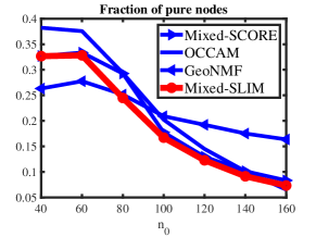
(a) Experiment 1(a)

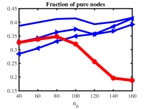
(b) Experiment 1(b)

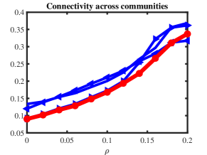
(c) Experiment 1(c)

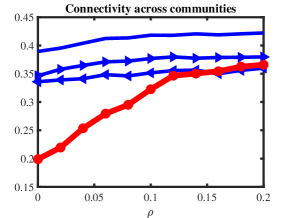
(d) Experiment 1(d)

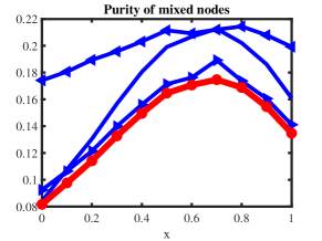
(e) Experiment 1(e)

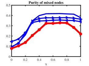
(f) Experiment 1(f)

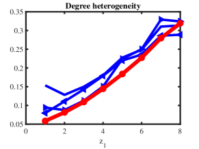
(g) Experiment 1(g)

(h) Experiment 1(h)

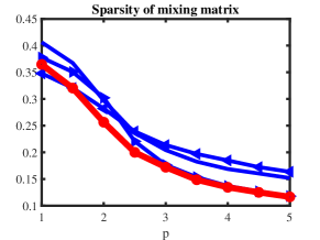
(i) Experiment 1(i)

(j) Experiment 1(j)

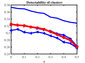
(k) Experiment 1(k)

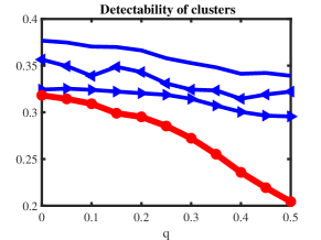
(l) Experiment 1(l)

Figure 1: Estimation errors of Experiment 1 (y-axis: $\sum_{i=1}^{n}n^{-1}\|\hat{\pi}_{i}-\pi_{i}\|_{1}$).

5.1.6 Detectability of clusters

We study how the detectability of clusters affects the behaviors of these mixed membership community detection methods in sub-experiments 1(k) and 1(l). In Experiment 1(k) and 1(l), set $(n,K,n_{0},x)=(500,4,75,0.2)$. For the top $4n_{0}$ nodes $\{1,2,\ldots,4n_{0}\}$, let these nodes be pure and let nodes $\{4n_{0}+1,4n_{0}+2,\ldots,500\}$ be mixed. Let all the mixed nodes have five different memberships $(x,x,x,1-3x),(x,x,1-3x,x),(x,1-3x,x,x),$ $(1-3x,x,x,x),(1/4,1/4,1/4,1/4)$. Let $q$ range in $\{0,0.05,0.1,\ldots,0.5\}$. The mixing matrix $P_{(kl)}$ is set as

$$P_{(kl)}=\begin{bmatrix}0.5+q&0.5&0.3&0.3\\ 0.5&0.5+q&0.3&0.3\\ 0.3&0.3&0.5+q&0.5\\ 0.3&0.3&0.5&0.5+q\\ \end{bmatrix}.$$

When $q=0$, the networks have only two communities, and as $q$ increases, the four communities become more distinguishable. Experiment 1(k) is the case under MMSB model, and Experiment 1(l) is under DCMM model.

The numerical results are given by the last two panels of Figure 1. Subfigure 1(k) suggests that Mixed-SLIM, Mixed-SCORE and GeoNMF share similar performances and they perform better than OCCAM under the MMSB setting. the proposed Mixed-SLIM significantly outperforms the other three methods under the DCMM setting.

5.2 Application to real-world datasets for community detection

In this section, six real-world network datasets with known labels information are analyzed to test the performances of our Mixed-SLIM methods for community detection. The six datasets can be downloaded from http://www-personal.umich.edu/~mejn/netdata/. For all the datasets, the true labels are suggested by the original authors, and they are regarded as the “ground truth” to investigate performances of Mixed-SLIM methods in this paper. Before comparing these methods, we take some preprocessing to remove nodes that may have mixed memberships for community detection. For the Polbooks data, nodes with labeled as “neutral” are removed. The five “independent” teams of Football data are removed. The smallest group with only 2 nodes in UKfaculty data is removed. A brief introduction of the six datasets are given in the Supplementary Materials. Table 1 presents some basic information about the six datasets. From Table 1, we can see that $d_{\mathrm{min}}$ and $d_{\mathrm{max}}$ are always quite different, which suggest a DCSBM case.

Table 1: Six real-world data sets with known label information.

#	Karate	Dolphins	Football	Polbooks	UKfaculty	Polblogs
$n$	34	62	110	92	79	1222
$K$	2	2	11	2	3	2
$d_{\mathrm{min}}$	1	1	7	1	2	1
$d_{\mathrm{max}}$	17	12	13	24	39	351

Table 2: Error rates on the six empirical data sets.

Methods	Karate	Dolphins	Football	Polbooks	UKfaculty	Polblogs
SCORE	0/34	0/62	5/110	1/92	1/79	58/1222
SLIM	1/34	0/62	6/110	2/92	1/79	51/1222
OCCAM	0/34	1/62	4/110	3/92	5/79	60/1222
Mixed-SCORE	0/34	2/62	4/110	3/92	6/79	60/1222
GeoNMF	0/34	1/62	5/110	3/92	4/79	64/1222
Mixed-SLIM	1/34	0/62	5/110	2/92	0/79	49/1222
Mixed-$\mathrm{SLIM}_{\tau}$	1/34	0/62	5/110	2/92	0/79	51/1222
Mixed-$\mathrm{SLIM}_{appro}$	1/34	0/62	5/110	2/92	0/79	50/1222
Mixed-$\mathrm{SLIM}_{\tau appro}$	1/34	0/62	5/110	2/92	0/79	51/1222

Table 2 records the error rates on the six real-world networks. The numerical results suggest that Mixed-SLIM methods enjoy satisfactory performances compared with SCORE, SLIM, OCCAM, Mixed-SCORE and GeoNMF when detecting the six empirical datasets. Especially, the number error for Mixed-SLIM on Polblogs network is 49, which is the smallest number error for this dataset in literature as far as we know.

5.3 Application to SNAP ego-networks for mixed membership community detection

The ego-networks dataset contains more than 1000 ego-networks from Facebook, Twitter, and GooglePlus. In an ego-network, all the nodes are friends of one central user and the friendship groups or circles (depending on the platform) set by this user can be used as ground truth communities. The SNAP ego-networks are open to public, and it can be downloaded from http://snap.stanford.edu/data/. It is applied to test the performances of OCCAM (Zhang et al., 2020) after some preprocessing. We obtain the SNAP ego-networks parsed by Yuan Zhang (the first author of the OCCAM method (Zhang et al., 2020)). The parsed SNAP ego-networks are slightly different from those used in Zhang et al. (2020). To get a better sense of what the different social networks look like and how different characteristics potentially affect performance of our Mixed-SLIM, we report the following summary statistics for each network: (1) number of nodes $n$ and number of communities $K$. (2) average node degree $\bar{d}$. (3) density $\sum_{i,j}A(i,j)/(n(n-1))$, i.e., the overall edge probability. (4) the proportion of overlapping nodes $r_{o}$, i.e., $r_{o}=\frac{\mathrm{number~{}of~{}nodes~{}with~{}mixed~{}membership}}{n}$. We report the means and standard deviations of these measures for each of the social networks in Table 3.

Table 3: Mean (SD) of summary statistics for ego-networks.

	#Networks	$n$	$K$	$\bar{d}$	Density	$r_{o}$
Facebook	7	236.57	3	30.61	0.15	0.009
	-	(228.53)	(1.15)	(29.41)	(0.058)	(0.008)
GooglePlus	58	433.22	2.22	66.81	0.18	0.005
	-	(327.70)	(0.46)	(65.2)	(0.11)	(0.005)
Twitter	255	60.64	2.63	17.87	0.33	0.02
	-	(30.77)	(0.83)	(9.97)	(0.17)	(0.008)

From Table 3, we see that Facebook and GooglePlus networks tend to be lager than Twitter networks, while Twitter networks are denser with larger density. Meanwhile, the proportions of overlapping nodes in Twitter networks tend to be larger than that of Facebook and GooglePlus networks. After obtaining the membership matrix $\Pi$ of each ego-network, to compute the mixed-Hamming error rate, we take a row-normalization step such that the sum of each row of $\Pi$ equals to 1.

We report the averaged mixed Hamming error rates and the corresponding standard deviations for our methods and other three competitors in Table 4. Obviously, Mixed-$\mathrm{SLIM}_{\tau appro}$ outperforms the other three Mixed-SLIM methods on all SNAP ego-networks and it significantly outperforms Mixed-SCORE, OCCAM and GeoNMF on GooglePlus and Twitter networks. Mixed-SLIM methods have smaller averaged mixed Humming error rates than Mixed-SCORE, OCCAM and GeoNMF on the GooglePlus networks and Twitter networks, while they perform slightly poorer than Mixed-SCORE on Facebook networks. Meanwhile, we also find that OCCAM and GeoNMF share similar performances on the ego-networks. It is interesting to find that the error rates on Twitter and GooglePlus networks are higher than error rates on Facebook which may because Twitter and GooglePlus networks have higher proportion of overlapping nodes than that of Facebook.

Table 4: Mean (SD) of mixed-Hamming error rates for ego-networks.

	Facebook	GooglePlus	Twitter
Mixed-SCORE	0.2496(0.1322)	0.3766(0.1053)	0.3087(0.1297)
OCCAM	0.2610(0.1367)	0.3564(0.1210)	0.2863(0.1403)
GeoNMF	0.2584(0.1262)	0.3507(0.1075)	0.2859(0.1293)
Mixed-SLIM	0.2521(0.1322)	0.3105(0.1216)	0.2706(0.1381)
Mixed-$\mathrm{SLIM}_{\tau}$	0.2507(0.1347)	0.3091(0.1184)	0.2656(0.1391)
Mixed-$\mathrm{SLIM}_{appro}$	0.2516(0.1331)	0.3161(0.1195)	0.2694(0.1339)
Mixed-$\mathrm{SLIM}_{\tau appro}$	0.2504(0.1326)	0.3088(0.1193)	0.2624(0.1363)

5.4 Discussion on the choices of $\tau$ and $T$

5.4.1 The effect of $\tau$ to Mixed-$\mathrm{\textbf{SLIM}}_{\tau}$

There is no practical criterion for choosing a best $\tau$ for Mixed-$\mathrm{SLIM}_{\tau}$ at present. Since we set $\tau=cd$ where $c$ is a nonnegative constant and $d$ should have the same order as the observed average degree, there are two directions to study the effect of $\tau$ to Mixed-$\mathrm{SLIM}_{\tau}$: One direction is changing $d$ when $c$ is fixed, and another direction is changing $c$ with fixed $d$.

For the first direction, we fix $c$ as 0.1, and let $d$ have three choices $\bar{d},d_{\mathrm{max}}$ and $\frac{d_{\mathrm{max}}+d_{\mathrm{min}}}{2}$. Table 5 reports the error rates of the six empirical datasets for different choice of $d$. Table 6 reports the Mean (SD) of mixed-Hamming error rates for SNAP ego-networks. Numerical results in these two tables show that Mixed-$\mathrm{SLIM}_{\tau}$ works satisfactory with three different choices $\bar{d},d_{\mathrm{max}}$ and $\frac{d_{\mathrm{max}}+d_{\mathrm{min}}}{2}$. We set $\bar{d}$ as the default $d$ in our Mixed-$\mathrm{SLIM}_{\tau}$ since it behaves slightly better than the other two choices.

Table 5: Error rates on the six data sets with different choice of $d$ for Mixed-$\mathrm{SLIM}_{\tau}$ when $\tau=0.1d$.

Methods	Karate	Dolphins	Football	Polbooks	UKfaculty	Polblogs
$\bar{d}$	1/34	0/62	5/110	2/92	0/79	51/1222
$d_{\mathrm{max}}$	1/34	0/62	5/110	2/92	1/79	56/1222
$\frac{d_{\mathrm{max}}+d_{\mathrm{min}}}{2}$	1/34	0/62	5/110	2/92	0/79	53/1222

Table 6: Mean (SD) of mixed-Hamming error rates with different choice of $d$ for Mixed-$\mathrm{SLIM}_{\tau}$ when $\tau=0.1d$.

	Facebook	GooglePlus	Twitter
$\bar{d}$	0.2507(0.1347)	0.3091(0.1184)	0.2656(0.1391)
$d_{\mathrm{max}}$	0.2521(0.1323)	0.3102(0.1203)	0.2632(0.1381)
$\frac{d_{\mathrm{max}}+d_{\mathrm{min}}}{2}$	0.2508(0.1335)	0.3104(0.1220)	0.2642(0.1370)

For the second direction, we fix $d$ as $\bar{d}$, and let $c$ range from 0 to 2 with step size 0.1. Figure 2 reports the error rates against $c$ on the six empirical datasets. Figure 3 reports the Mean of mixed-Hamming error rates against $c$ on SNAP ego-networks. These two figures suggest that Mixed-$\mathrm{SLIM}_{\tau}$ is robust on the choice of $c$ as long as $\tau$ is in the same order as the observed average degree. Combining with numerical results of Tables 5, 6 and Figures 2, 3, we conclude that Mixed-$\mathrm{SLIM}_{\tau}$ is insensitive to the choice of $\tau$.

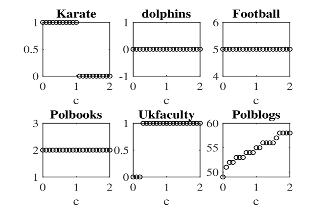
Figure 2: Number errors on the six empirical datasets for Mixed-$\mathrm{SLIM}_{\tau}$ when $\tau=c\bar{d}$, where $c$ is in $\{0,0.1,0.2,\ldots,2\}$. x-axis: $c$, y-axis: number errors.

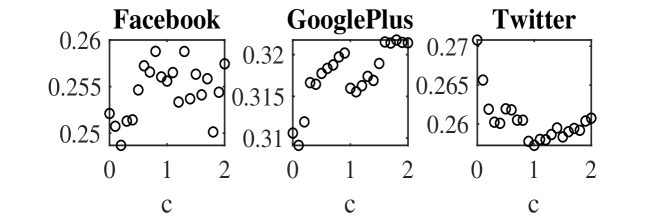
Figure 3: Mean of mixed-Hamming error rates on SNAP ego-networks for Mixed-$\mathrm{SLIM}_{\tau}$ when $\tau=c\bar{d}$, where $c$ is in $\{0,0.1,0.2,\ldots,2\}$. x-axis: $c$, y-axis: mean of mixed-Hamming error rates .

5.4.2 The effect of $T$ to Mixed-$\mathrm{\textbf{SLIM}}_{appro}$

We study the effect of $T$ to Mixed-$\mathrm{SLIM}_{appro}$ by changing $T$ from 1 to 20 on these empirical datasets. The respective numerical results are shown in Figures 4 and 5. From these figures we see that Mixed-$\mathrm{SLIM}_{appro}$ successfully detect these datasets except for Polblogs when $T$ is 1 or 2. These results suggest that Mixed–$\mathrm{SLIM}_{appro}$ is insensitive to the choice of $T$ as long as it is larger than or equal to 3.

Meanwhile, as discussed in Jing et al. (2021), when $T$ is too large, $\hat{D}^{-T}A^{T}$ no longer contains any block structure, and all nodes merge into one giant community since $\hat{D}^{-T}$ is nearly singular for large $T$. Therefore the ideal choice for $T$ should not be too large as 10 for Mxied-$\mathrm{SLIM}_{appro}$ in practice.

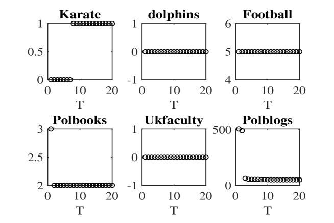
Figure 4: Number errors on six empirical networks for Mixed-$\mathrm{SLIM}_{appro}$ based on different choice of $T$, where $T$ is in $\{1,2,\ldots,20\}$. x-axis: $T$, y-axis: number errors.

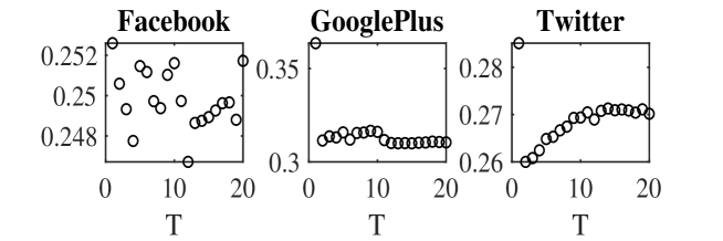
Figure 5: Mean of mixed-Hamming error rates on SNAP ego-networks for Mixed-$\mathrm{SLIM}_{appro}$ based on different choice of $T$, where $T$ is in $\{1,2,\ldots,20\}$. x-axis: $T$, y-axis: mean of mixed-Hamming error rates.

6 Discussion

This paper makes one major contribution: modified SLIM methods to mixed membership community detection under the DCMM model. When dealing with large networks in practice, we apply Mixed-$\mathrm{SLIM}_{appro}$ and its regularized version Mixed-$\mathrm{SLIM}_{\tau appro}$. We showed the estimation consistency of the regularized version Mixed-$\mathrm{SLIM}_{\tau}$ under the DCMM model. Meanwhile, Mixed-SLIM methods are robust to the choice of the two tuning parameters $\tau$ and $T$. But similar as Jing et al. (2021), the proposed methods are sensitive to the choice of $\alpha$. And we leave the study of choosing optimal $\alpha$ theoretically in future work. Both simulation and empirical results for community detection and mixed membership community detection demonstrate that Mixed-SLIM methods enjoy satisfactory performances and they perform better than most of the benchmark methods.

Building the theoretical framework for Mixed-$\mathrm{SLIM}_{appro}$ and Mixed-$\mathrm{SLIM}_{\tau appro}$ is challenging and interesting, and we leave it as future work. In Mixed-SLIM methods, the SLIM matrix is computed by $(I-\alpha\hat{D}_{\tau}^{-1}A_{\tau})^{-1}$, we wonder that whether there exists an optimal parameter $\beta_{0}$ such that Mixed-SLIM methods designed based on the new SLIM matrix $(I-\alpha\hat{D}_{\tau}^{-\beta_{0}}A_{\tau})^{-1}$ outperform those designed based on $(I-\alpha\hat{D}_{\tau}^{-\beta}A_{\tau})^{-1}$ for any $\beta$ both theoretically and empirically. In Jin et al. (2017) they applied VH algorithm for vertexes hunting, while in this paper we applied K-medians clustering algorithm, thus it may be interesting to use VH algorithm in Mixed-SLIM methods. It remains unclear how to estimate the number of communities K, and we wonder that whether the SLIM matrix and its regularized one can be applied for estimating $K$ both theoretically and empirically. In the Post-PCA Normalization step in our mixed-SLIM, similar as that in Jin et al. (2017), we can compute an $n\times(K-1)$ matrix of entry-wise ratios $\hat{R}$, but such normalization makes it tedious and challenging for theoretical analysis. For reasons of space, we leave studies of these problems to the future.

References

- (1)
- Airoldi et al. (2008) Airoldi, E. M., Blei, D. M., Fienberg, S. E. & Xing, E. P. (2008), ‘Mixed membership stochastic blockmodels’, Journal of Machine Learning Research 9, 1981–2014.
- Anandkumar et al. (2014) Anandkumar, A., Ge, R., Hsu, D. & Kakade, S. M. (2014), ‘A tensor approach to learning mixed membership community models’, Journal of Machine Learning Research 15(1), 2239–2312.
- Bedi & Sharma (2016) Bedi, P. & Sharma, C. (2016), ‘Community detection in social networks’, Wiley Interdisciplinary Reviews: Data Mining and Knowledge Discovery 6(3), 115–135.
- Chen et al. (2018) Chen, Y., Li, X. & Xu, J. (2018), ‘Convexified modularity maximization for degree-corrected stochastic block models’, Annals of Statistics 46(4), 1573–1602.
- Decelle et al. (2011) Decelle, A., Krzakala, F., Moore, C. & Zdeborová, L. (2011), ‘Asymptotic analysis of the stochastic block model for modular networks and its algorithmic applications’, Physical Review E 84(6), 066106.
- Dunne et al. (2002) Dunne, J. A., Williams, R. J. & Martinez, N. D. (2002), ‘Food-web structure and network theory: The role of connectance and size’, Proceedings of the National Academy of ences of the United States of America 99(20), 12917.
- Gao et al. (2010) Gao, J., Liang, F., Fan, W., Wang, C., Sun, Y. & Han, J. (2010), On community outliers and their efficient detection in information networks, in ‘Proceedings of the 16th ACM SIGKDD International Conference on Knowledge Discovery and Data Mining’, pp. 813–822.
- Goldenberg & Anna (2010) Goldenberg & Anna (2010), ‘A survey of statistical network models’, Foundations & Trends in Machine Learning 2(2), 129–233.
- Gulikers et al. (2018) Gulikers, L., Lelarge, M. & Massoulié, L. (2018), ‘An impossibility result for reconstruction in the degree-corrected stochastic block model’, Annals of Applied Probability 28(5), 3002–3027.
- Holland et al. (1983) Holland, P. W., Laskey, K. B. & Leinhardt, S. (1983), ‘Stochastic blockmodels: First steps’, Social Networks 5(2), 109–137.
- Jin (2015) Jin, J. (2015), ‘Fast community detection by SCORE’, Annals of Statistics 43(1), 57–89.
- Jin & Ke (2017) Jin, J. & Ke, Z. T. (2017), ‘A sharp lower bound for mixed-membership estimation’, arXiv preprint arXiv:1709.05603 .
- Jin et al. (2017) Jin, J., Ke, Z. T. & Luo, S. (2017), ‘Estimating network memberships by simplex vertex hunting’, arXiv preprint arXiv:1708.07852 .
- Jing et al. (2021) Jing, B., Li, T., Ying, N. & Yu, X. (2021), ‘Community detection in sparse networks using the symmetrized laplacian inverse matrix (slim)’, Statistica Sinica .
- Karrer & Newman (2011a) Karrer, B. & Newman, M. E. (2011a), ‘Stochastic blockmodels and community structure in networks’, Physical Review E 83(1), 016107.
- Karrer & Newman (2011b) Karrer, B. & Newman, M. E. J. (2011b), ‘Stochastic blockmodels and community structure in networks’, Physical Review E 83(1), 16107.
- Lancichinetti & Fortunato (2009) Lancichinetti, A. & Fortunato, S. (2009), ‘Community detection algorithms: a comparative analysis’, Physical Review E 80(5), 056117.
- Latouche et al. (2011) Latouche, P., Birmelé, E. & Ambroise, C. (2011), ‘Overlapping stochastic block models with application to the french political blogosphere’, Annals of Applied Statistics 5(1), 309–336.
- Leskovec et al. (2010) Leskovec, J., Lang, K. J. & Mahoney, M. (2010), Empirical comparison of algorithms for network community detection, in ‘Proceedings of the 19th International Conference on World Wide Web’, pp. 631–640.
- Leskovec & Mcauley (2012) Leskovec, J. & Mcauley, J. J. (2012), ‘Learning to discover social circles in ego networks’, Advances in Neural Information Processing Systems 25 pp. 539–547.
- Lin et al. (2012) Lin, W., Kong, X., Yu, P. S., Wu, Q., Jia, Y. & Li, C. (2012), Community detection in incomplete information networks, in ‘Proceedings of the 21st International Conference on World Wide Web’, pp. 341–350.
- Mao et al. (2017) Mao, X., Sarkar, P. & Chakrabarti, D. (2017), ‘On mixed memberships and symmetric nonnegative matrix factorizations’, International Conference on Machine Learning pp. 2324–2333.
- Mao et al. (2020) Mao, X., Sarkar, P. & Chakrabarti, D. (2020), ‘Estimating mixed memberships with sharp eigenvector deviations’, Journal of American Statistical Association pp. 1–13.
- Newman (2004) Newman, M. E. J. (2004), ‘Coauthorship networks and patterns of scientific collaboration’, Proceedings of the National Academy of Sciences 101(suppl 1), 5200–5205.
- Notebaart et al. (2006) Notebaart, R. A.and van Enckevort, F. H., Francke, C., Siezen, R. J. & Teusink, B. (2006), ‘Accelerating the reconstruction of genome-scale metabolic networks’, BMC Bioinformatics 7, 296.
- Pizzuti (2008) Pizzuti, C. (2008), Ga-net: A genetic algorithm for community detection in social networks, in ‘International Conference on Parallel Problem Solving from Nature’, Springer, pp. 1081–1090.
- Qin & Rohe (2013) Qin, T. & Rohe, K. (2013), ‘Regularized spectral clustering under the degree-corrected stochastic blockmodel’, Advances in Neural Information Processing Systems 26 pp. 3120–3128.
- Qing & Wang (2020a) Qing, H. & Wang, J. (2020a), ‘Estimating network memberships by mixed regularized spectral clustering’, arXiv preprint arXiv:2011.12239 .
- Qing & Wang (2020b) Qing, H. & Wang, J. (2020b), ‘An improved spectral clustering method for community detection under the degree-corrected stochastic blockmodel’, arXiv preprint arXiv:2011.06374 .
- Scott & Carrington (2014) Scott, J. & Carrington, P. J. (2014), The SAGE handbook of social network analysis, London: SAGE Publications.
- Su et al. (2010) Su, G., Kuchinsky, A., Morris, J. H., States, D. J. & Meng, F. (2010), ‘Glay: community structure analysis of biological networks’, Bioinformatics 26(24), 3135–3137.
- Wang et al. (2015) Wang, C., Tang, W., Sun, B., Fang, J. & Wang, Y. (2015), Review on community detection algorithms in social networks, in ‘2015 IEEE International Conference on Progress in Informatics and Computing (PIC)’, IEEE, pp. 551–555.
- Zhang et al. (2020) Zhang, Y., Levina, E. & Zhu, J. (2020), ‘Detecting overlapping communities in networks using spectral methods’, SIAM Journal on Mathematics of Data Science 2(2), 265–283.
- Zhao et al. (2012) Zhao, Y., Levina, E. & Zhu, J. (2012), ‘Consistency of community detection in networks under degree-corrected stochastic block models’, Annals of Statistics 40(4), 2266–2292.