Ion-acoustic rogue waves in double pair plasma having non-extensive particles

Abstract

The modulational instability (MI) of ion-acoustic (IA) waves (IAWs) and associated IA rogue waves (IARWs) in double pair plasma containing non-extensive electrons, iso-thermal positrons, negatively and positively charged ions have been governed by the standard nonlinear Schrödinger equation (NLSE). It has been figured out from the numerical study of NLSE that the plasma system holds modulationally stable (unstable) region in which the dispersive and nonlinear coefficients of the NLSE have the opposite (same) signs. It is also found that the fundamental features of IAWs (viz., MI criteria, amplitude and width of the IARWs, etc.) are rigorously organized by the plasma parameters such as mass, charge state, and number density of the plasma components. The existing outcomes of our present study should be helpful for understanding the nonlinear features of IAWs (viz., MI and IARWs) in both laboratory and space plasmas.

1 Introduction

Double pair plasma (DPP) is characterised as fully ionized gas having electrons, positron as well as positive and negative ions, and is believed to exist in astrophysical environments such as Van Allen radiation belt and near the polar cap of fast rotation neutron stars [1], solar atmosphere [2], D-region ($H^{+},O_{2}^{-}$) and F-region ($H^{+},H^{-}$) of the earths’s ionosphere [3], upper region of Titan’s atmosphere [4] and also in laboratory environments [5, 6, 7, 8, 9, 10]. A number of authors [11, 12, 13] studied ion-acoustic (IA) waves (IAWs) and associated nonlinear electrostatic structures namely, solitons, shocks, rogue waves, and double layers in the DPP.

Maxwellian distribution function is one of the most widely used velocity distribution functions of particles to describe the dynamics of the iso-thermal particles. But it has been observed that the characteristics of majority of particles in the space [14] and laboratory plasma environments [15] are departed from the Maxwellian distribution. So, to narrate the non-Maxwellian particles, Renyi [16] first recognized the modification of Maxwellian distribution, and finally, Tsallis [17] generalized the non-extensive $q$-distribution. It is noted that the index $q$ in the non-extensive $q$-distribution characterizes the degree of non-extensivity of the particles [18]. Shalini et al. [19] studied IAWs in non-extensive plasma having two-temperature electrons, and observed that the width of the first and second order IA rogue waves (IARWs) associated with IAWs decreases with increasing the value of $q$ but the amplitude of the first and second-order IARWs associated with IAWs is remain constant. Tribeche et al. [20] investigated electrostatic solitary waves in presence of the non-extensive electrons, and found that the amplitude of the potential increases with non-extensive parameter. Hafez and Talukder [21] examined the propagation of the nonlinear electrostatic waves in a three-component non-extensive plasma having inertialess non-extensive electrons and positrons, and inertial ions, and reported that the amplitude of the soliton increases with increasing temperature of the non-extensive electron.

The investigation of the modulational instability (MI) [22, 23, 24, 25, 26, 27] and associated nonlinear features of wave is one of the most important research areas for plasma physicists. It is noteworthy that the MI of the wave is considered to be the primary reason for the formation of massive and gigantic rogue waves (RWs) [28]. Rogue wave, which is the rational solution of the standard nonlinear Schrödinger equation (NLSE) [28, 29, 30, 31], is a short-lived phenomenon which emerges from nowhere and disappears without a trace [29]. A number of authors have investigated the MI of IAWs by considering the non-extensive particles [32, 33, 34]. Bains et al. [32] studied the MI of IAWs in presence of non-extensive electrons, and demonstrated that the critical wave number ($k_{c}$) at which the instability sets in increases with the increase in the value of $q$ ($q>0$). Bouzit et al. [33] investigated the stability conditions of IAWs in presence of non-extensive non-thermal electrons. Eslami et al. [34] investigated the MI of IAWs in electron-positron-ion plasma having non-extensive electrons and positrons, and observed that the $k_{c}$ decreases with $q$ for $q<0$ while increases with $q$ for $q>0$. To the best knowledge of the authors, no attempt has been made to investigate the MI of the IAWs and associated IARWs in a four-component plasma containing inertial positively and negatively charged ions, and inertialess non-extensive electrons, and iso-thermal positrons. Therefore, it is a rational fascination to examine the influence of non-extensive electrons and iso-thermal positrons on the MI of IAWs and associated IARWs in a four-component DPP.

The manuscript is organized as the following pattern: The model equations are presented in Sec. 2. The derivation of the NLSE is shown in Sec. 3. The stability of IAWs is provided in Sec. 4. The IARWs is demonstrated in Sec. 5. Finally, a conclusion is given in Sec. 6.

2 Model Equations

We consider the propagation of IAWs in a collisionless, fully ionized, unmagnetized plasma system consisting of warm negative ions, symbolized by $n_{-i}$ (charge $q_{-i}=-Z_{-i}e$; mass $m_{-i}$), warm positive ions, denoted by $n_{+i}$ (charge $q_{+i}=Z_{+i}e$; mass $m_{+i}$), non-extensive $q$-distributed electrons, identified by $n_{e}$ (charge $q_{e}=-e$; mass $m_{e}$), and iso-thermal positrons, expressed by $n_{p}$ (charge $q_{p}=+e$; mass $m_{p}$); where $Z_{-i}$ ($Z_{+i}$) is the charge state of the negatively (positively) charged ion, and $e$ being the magnitude of the charge of the electron. The charge neutrality condition of our present model can be written as $n_{p0}+Z_{+i}n_{+i0}=n_{e0}+Z_{-i}n_{-i0}$. Now, the normalized equations can be given in the following form

$$\frac{\partial n_{-i}}{\partial t}+\frac{\partial}{\partial x}(n_{-i}u_{-i})=0,$$ (1)

$$\frac{\partial u_{-i}}{\partial t}+u_{-i}\frac{\partial u_{-i}}{\partial x}+\lambda_{1}n_{-i}\frac{\partial n_{-i}}{\partial x}=\frac{\partial\phi}{\partial x},$$ (2)

$$\frac{\partial n_{+i}}{\partial t}+\frac{\partial}{\partial x}(n_{+i}u_{+i})=0,$$ (3)

$$\frac{\partial u_{+i}}{\partial t}+u_{+i}\frac{\partial u_{+i}}{\partial x}+\lambda_{3}n_{+i}\frac{\partial n_{+i}}{\partial x}=-\lambda_{2}\frac{\partial\phi}{\partial x},$$ (4)

$$\frac{\partial^{2}\phi}{\partial x^{2}}=\lambda_{4}n_{e}+n_{-i}-(1+\lambda_{4}-\lambda_{5})n_{p}-\lambda_{5}n_{+i},\$$ (5)

where $n_{-i}$, $n_{+i}$, $n_{e}$, and $n_{p}$ are normalized by $n_{-i0}$, $n_{+i0}$, $n_{e0}$, and $n_{p0}$, respectively; $u_{-i}$ and $u_{+i}$ indicate the negatively and positively charged ion fluid, respectively, normalized by the IA wave speed $C_{-i}=(Z_{-i}k_{B}T_{e}/m_{-i})^{1/2}$ (with $k_{B}$ being the Boltzmann constant and $T_{e}$ being the temperature of the electron); $\phi$ denoted as the electrostatic wave potential, normalized by $k_{B}T_{e}/e$; the time and space variables are, respectively normalized by $\omega_{-ip}^{-1}=(m_{-i}/4\pi e^{2}Z_{-i}^{2}n_{-i0})^{1/2}$ and $\lambda_{-i}=(k_{B}T_{e}/4\pi e^{2}Z_{-i}n_{-i0})^{1/2}$. The pressure term of the ion can be represented as $P_{-i}=P_{-i0}(N_{-i}/n_{-i0})^{\gamma}$ with $P_{-i0}=n_{-i0}k_{B}T_{-i}$; where $P_{-i0}$ ($T_{-i}$) being the equilibrium pressure (temperature) of the negatively charged ion, and $P_{+i}=P_{+i0}(N_{+i}/n_{+i0})^{\gamma}$ with $P_{+i0}=n_{+i0}k_{B}T_{+i}$; where $P_{+i0}$ ($T_{+i}$) being the equilibrium pressure (temperature) of the positively charged ion, respectively, and $\gamma=(N+2)/N$ (where $N$ recognized as the degree of freedom and for one-dimensional case $N=1$, so $\gamma=3$). Other parameters can be defined as $\lambda_{1}=3T_{-i}/Z_{-i}T_{e}$, $\lambda_{2}=Z_{+i}m_{-i}/Z_{-i}m_{+i}$, $\lambda_{3}=3T_{+i}m_{-i}/Z_{-i}m_{+i}T_{e}$, $\lambda_{4}=n_{e0}/Z_{-i}n_{-i0}$, and $\lambda_{5}=Z_{+i}n_{+i0}/Z_{-i}n_{-i0}$. Now, the number densities of the non-extensive $q-$distributed [17, 35] electron and iso-thermally distributed [36, 37] positron can be represented by the following normalized equations

$$n_{e}=[1+(q-1)\phi]^{\frac{q+1}{2(q-1)}},$$ (6)

$$n_{p}=\mbox{exp}(-\lambda_{6}\phi),\$$ (7)

where $\lambda_{6}=T_{e}/T_{p}$ (with $T_{p}$ being the temperature of the iso-thermally distributed positron and $T_{e}>T_{p}$). The parameter $q$, generally known as entropic index which quantifies the degree of non-extensivity. It is noteworthy that when $q=1$, the entropy reduces to standard Maxwell-Boltzmann distribution. On the other hand, in the limits $q>0$ ($q<0$), the entropy shows sub-extensivity (super-extensivity). Now, by substituting Eqs. $(6)$ and $(7)$ into Eq. $(5)$ and expanding up to third order in $\phi$, we can draw up as

$$\frac{\partial^{2}\phi}{\partial x^{2}}+1+\lambda_{5}n_{+i}=\lambda_{5}+n_{-i}+M_{1}\phi+M_{2}\phi^{2}+M_{3}\phi^{3}+\cdot\cdot\cdot,\$$ (8)

where

$$M_{1}=[\lambda_{4}(q+1)+2\lambda_{6}(1+\lambda_{4}-\lambda_{5})]/2,$$

$$M_{2}=[\lambda_{4}(q+1)(3-q)-4\lambda_{6}^{2}(1+\lambda_{4}-\lambda_{5})]/8,$$

$$M_{3}=[\lambda_{4}(q+1)(q-3)(3q-5)+8\lambda_{6}^{3}(1+\lambda_{4}-\lambda_{5})]/48.\$$

It is noted that the terms containing $M_{1}$, $M_{2}$, and $M_{3}$ in Eq. (8) are due to the contribution of the non-extensive $q$-distributed electrons and iso-thermal positrons.

3 Derivation of the NLSE

To study the MI of the IAWs, first we want to construct the NLSE by employing the reductive perturbation method. In that case, the stretched co-ordinates can be written in the following fashion [35, 38, 39, 40, 41, 42]

$$\xi=\epsilon(x-v_{g}t),$$ (9)

$$\tau=\epsilon^{2}t,\$$ (10)

where $v_{g}$ is the group speed and $\epsilon$ is a small parameter. After that the dependent variables can be represented as [35, 38, 39, 40, 41, 42]

$$\Pi(x,t)=\Pi_{0}+\sum_{m=1}^{\infty}\epsilon^{(m)}\sum_{l=-\infty}^{\infty}\Pi_{l}^{(m)}(\xi,\tau)M,\$$ (11)

where $\Pi_{il}^{(m)}=[n_{-il}^{m},u_{-il}^{m},n_{+il}^{m},u_{+il}^{m},\phi_{il}^{m}]$, $\Pi_{0}=[1,0,1,0,0]^{T}$, $M=\mbox{exp}[il(kx-\omega t)]$, and $k~{}(\omega)$ is real variables representing the carrier wave number (frequency). The derivative operators can be showed as

$$\frac{\partial}{\partial t}\rightarrow\frac{\partial}{\partial t}-\epsilon v_{g}\frac{\partial}{\partial\xi}+\epsilon^{2}\frac{\partial}{\partial\tau},$$ (12)

$$\frac{\partial}{\partial x}\rightarrow\frac{\partial}{\partial x}+\epsilon\frac{\partial}{\partial\xi}.\$$ (13)

Now, by substituting Eqs. (9)$-$(13) into Eqs. (1)$-$(4), and (8), and collecting power term of $\epsilon$, the first order ($m=1$ with $l=1$) shortened equations can be presented as

$$n_{-i1}^{(1)}=\frac{k^{2}}{S}\phi_{1}^{(1)},$$ (14)

$$u_{-i1}^{(1)}=\frac{k\omega}{S}\phi_{1}^{(1)},$$ (15)

$$n_{+i1}^{(1)}=\frac{\lambda_{2}k^{2}}{A}\phi_{1}^{(1)},$$ (16)

$$u_{+i1}^{(1)}=\frac{\lambda_{2}\omega k}{A}\phi_{1}^{(1)},\$$ (17)

where $S=\lambda_{1}k^{2}-\omega^{2}$ and $A=\omega^{2}-\lambda_{3}k^{2}$. These equations provide the dispersion relation of IAWs in the following form

$$\omega^{2}=\frac{I\pm\sqrt{I^{2}-4UJ}}{2U},$$ (18)

where $I=(\lambda_{1}k^{2}+\lambda_{3}k^{2}+\lambda_{1}M_{1}+\lambda_{3}M_{1}+\lambda_{2}\lambda_{5}+1)$, $U=(k^{2}+M_{1})/k^{2}$, and $J=k^{2}(\lambda_{1}\lambda_{3}k^{2}+\lambda_{1}\lambda_{3}M_{1}+\lambda_{3}+\lambda_{1}\lambda_{2}\lambda_{5})$. However, to obtain the real and positive values of $\omega$, the conditions $I^{2}>4UJ$ must be maintained. It is noted that the positive and negative signs in Eq. (18) resembled to the fast ($\omega_{f}$) and slow ($\omega_{s}$) IA modes, respectively. The second order ($m=2$ with $l=1$) equations and with the compatibility condition, we can be written the group speed of the IAWs

$$v_{g}=\frac{(L+\lambda_{1}A^{2}k^{2}+A^{2}\omega^{2}-2A^{2}S^{2}-SA^{2})}{2\omega k(A^{2}+\lambda_{2}\lambda_{5}S^{2})},\$$ (19)

where $L=\lambda_{2}\lambda_{3}\lambda_{5}k^{2}S^{2}+\lambda_{2}\lambda_{5}\omega^{2}S^{2}+\lambda_{2}\lambda_{5}AS^{2}$. Now, the co-efficient of $\epsilon$ (when $m=2$ with $l=2$) yield the second-order harmonic amplitudes are found to be proportional to $|\phi_{1}^{(1)}|^{2}$

$$n_{-i2}^{(2)}=M_{4}|\phi_{1}^{(1)}|^{2},$$ (20)

$$u_{-i2}^{(2)}=M_{5}|\phi_{1}^{(1)}|^{2},$$ (21)

$$n_{+i2}^{(2)}=M_{6}|\phi_{1}^{(1)}|^{2},$$ (22)

$$u_{+i2}^{(2)}=M_{7}|\phi_{1}^{(1)}|^{2},$$ (23)

$$\phi_{2}^{(2)}=M_{8}|\phi_{1}^{(1)}|^{2},\$$ (24)

where

$$M_{4}=\frac{2M_{8}k^{2}S^{2}-3\omega^{2}k^{4}-\lambda_{1}k^{6}}{2S^{3}},$$

$$M_{5}=\frac{\omega M_{4}S^{2}-\omega k^{4}}{kS^{2}},$$

$$M_{6}=\frac{2\lambda_{2}M_{8}A^{2}k^{2}+3\lambda_{2}^{2}\omega^{2}k^{4}+\lambda_{3}\lambda_{2}^{2}k^{6}}{2A^{3}},$$

$$M_{7}=\frac{\omega M_{6}A^{2}-\omega\lambda_{2}^{2}k^{4}}{kA^{2}},$$

$$M_{8}=\frac{2M_{2}A^{3}S^{3}-3\lambda_{5}\lambda_{2}^{2}\omega^{2}S^{3}k^{4}-M_{9}}{M_{10}},$$

$$M_{9}=3\omega^{2}A^{3}k^{4}+\lambda_{3}\lambda_{5}\lambda_{2}^{2}S^{3}k^{6}+\lambda_{1}A^{3}k^{6},$$

$$M_{10}=2A^{2}S^{2}(S\lambda_{2}\lambda_{5}k^{2}-4k^{2}AS-M_{1}AS-Ak^{2}).\$$

Next, consider the image for $m=3$ with $l=0$ and $m=2$ with $l=0$, which margined the zeroth harmonic modes. In such a way we can get the following results

$$n_{-i0}^{(2)}=M_{11}|\phi_{1}^{(1)}|^{2},$$ (25)

$$u_{-i0}^{(2)}=M_{12}|\phi_{1}^{(1)}|^{2},$$ (26)

$$n_{+i0}^{(2)}=M_{13}|\phi_{1}^{(1)}|^{2},$$ (27)

$$u_{+i0}^{(2)}=M_{14}|\phi_{1}^{(1)}|^{2},$$ (28)

$$\phi_{0}^{(2)}=M_{15}|\phi_{1}^{(1)}|^{2},\$$ (29)

where

$$M_{11}=\frac{2\omega v_{g}k^{3}+\lambda_{1}k^{4}+k^{2}\omega^{2}-M_{15}S^{2}}{S^{2}(v_{g}^{2}-\lambda_{1})},$$

$$M_{12}=\frac{M_{11}v_{g}S^{2}-2\omega k^{3}}{S^{2}},$$

$$M_{13}=\frac{\lambda_{2}M_{15}A^{2}+\lambda_{3}\lambda_{2}^{2}k^{4}+\lambda_{2}^{2}\omega^{2}k^{2}+2\omega v_{g}\lambda_{2}^{2}k^{3}}{A^{2}(v_{g}^{2}-\lambda_{3})},$$

$$M_{14}=\frac{M_{13}v_{g}A^{2}-2\omega\lambda_{2}^{2}k^{3}}{A^{2}},$$

$$M_{15}=\frac{A^{2}(v_{g}^{2}-\lambda_{3})(2\omega v_{g}k^{3}+\lambda_{1}k^{4}+\omega^{2}k^{2})+M_{16}}{A^{2}S^{2}v_{g}^{2}+M_{17}},$$

$$M_{16}=2M_{2}A^{2}S^{2}(v_{g}^{2}-\lambda_{1})(v_{g}^{2}-\lambda_{3})-(v_{g}^{2}-\lambda_{1})$$

$$S^{2}(2\lambda_{5}\omega v_{g}\lambda_{2}^{2}k^{3}+\lambda_{3}\lambda_{5}\lambda_{2}^{2}k^{4}+\lambda_{5}\lambda_{2}^{2}\omega^{2}k^{2}),$$

$$M_{17}=A^{2}S^{2}[\lambda_{2}\lambda_{5}(v_{g}^{2}-\lambda_{1})-\lambda_{3}-M_{1}(v_{g}^{2}-\lambda_{1})(v_{g}^{2}-\lambda_{3})].\$$

Lastly, the third-order harmonic modes ($m=3$ with $l=1$), with the assistance of Eqs. (14)$-$(29), represent a complete set of equations, which can be transformed to the NLSE:

$$i\frac{\partial\Phi}{\partial\tau}+P\frac{\partial^{2}\Phi}{\partial\xi^{2}}+Q|\Phi|^{2}\Phi=0,\$$ (30)

where $\Phi=\phi_{1}^{(1)}$ for simplicity. In Eq. (30), $P$ is the dispersion co-efficient, which can be written as

$$P=\frac{4\lambda_{2}\lambda_{5}\omega^{2}k^{2}v_{g}^{2}S^{3}+4\lambda_{1}\omega v_{g}A^{3}k^{3}+4kv_{g}\omega^{3}A^{3}+M_{18}}{2\omega ASk^{2}(A^{2}+\lambda_{2}\lambda_{5}S^{2})},\$$

$$M_{18}=2\lambda_{2}\lambda_{3}\lambda_{5}\omega^{2}k^{2}S^{3}+\lambda_{2}\lambda_{5}\lambda_{3}^{2}S^{3}k^{4}+\lambda_{1}Sk^{2}A^{3}$$

$$+\lambda_{2}\lambda_{5}S^{3}\omega^{4}+\lambda_{2}\lambda_{3}\lambda_{5}Ak^{2}S^{3}-4\lambda_{2}\lambda_{5}kv_{g}\omega^{3}S^{3}$$

$$-4\lambda_{2}\lambda_{3}\lambda_{5}\omega v_{g}k^{3}S^{3}-4\omega^{2}k^{2}v_{g}^{2}A^{3}-\lambda_{1}^{2}A^{3}k^{4}$$

$$-2\lambda_{1}\omega^{2}k^{2}A^{3}-Sk^{2}v_{g}^{2}A^{3}-A^{3}\omega^{4}$$

$$-\lambda_{2}\lambda_{5}Ak^{2}v_{g}^{2}S^{3}-A^{3}S^{3},\$$

and $Q$ is the nonlinear co-efficient, which can be written as

$$Q=\frac{3M_{3}A^{2}S^{2}+2M_{2}M_{8}A^{2}S^{2}+2M_{2}M_{15}A^{2}S^{2}-M_{19}}{2\omega k^{2}(A^{2}+\lambda_{2}\lambda_{5}S^{2})},\$$

where

$$M_{19}=2\omega M_{5}A^{2}k^{3}+2\lambda_{2}\lambda_{5}\omega M_{7}S^{2}k^{3}+2\omega M_{12}A^{2}k^{3}$$

$$+2\lambda_{2}\lambda_{5}\omega M_{14}S^{2}k^{3}+\lambda_{1}M_{4}A^{2}k^{4}+M_{4}\omega^{2}A^{2}k^{2}$$

$$+\lambda_{2}\lambda_{3}\lambda_{5}M_{6}S^{2}k^{4}+\lambda_{2}\lambda_{5}M_{6}\omega^{2}k^{2}S^{2}+M_{11}\omega^{2}A^{2}k^{2}$$

$$+\lambda_{1}M_{11}A^{2}k^{4}+\lambda_{2}\lambda_{5}M_{13}\omega^{2}k^{2}S^{2}+\lambda_{2}\lambda_{3}\lambda_{5}M_{13}S^{2}k^{4}$$

It may be noted here that both $P$ and $Q$ are directly depend on different parameters namely $\lambda_{1}$, $\lambda_{2}$, $\lambda_{3}$, $\lambda_{4}$, $\lambda_{5}$, $\lambda_{6}$, $q$, and are indirectly depend on mass, number density, temperature, and charge state of the different plasma components.

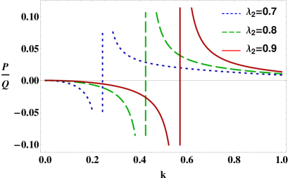
Figure 1: The variation of $P/Q$ with $k$ for different values of $\lambda_{2}$ when $\lambda_{1}=0.007$, $\lambda_{3}=0.07$, $\lambda_{4}=1.8$, $\lambda_{5}=1.5$, $\lambda_{6}=1.7$, $q=1.4$, and $\omega\equiv\omega_{f}$.

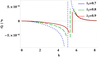
Figure 2: The variation of $P/Q$ with $k$ for different values of $\lambda_{2}$ when $\lambda_{1}=0.007$, $\lambda_{3}=0.07$, $\lambda_{4}=1.8$, $\lambda_{5}=1.5$, $\lambda_{6}=1.7$, $q=1.4$, and $\omega\equiv\omega_{s}$.

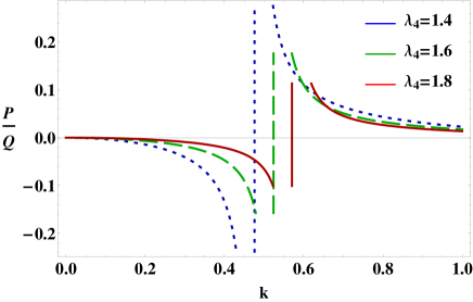
Figure 3: The variation of $P/Q$ with $k$ for different values of $\lambda_{4}$ when $\lambda_{1}=0.007$, $\lambda_{2}=1.2$, $\lambda_{3}=0.07$, $\lambda_{5}=1.5$, $\lambda_{6}=1.7$, $q=1.4$, and $\omega\equiv\omega_{f}$.

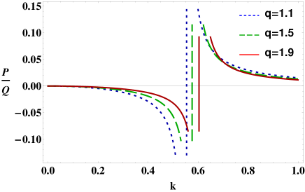
Figure 4: The variation of $P/Q$ with $k$ for different values of $q$ when $\lambda_{1}=0.007$, $\lambda_{2}=1.2$, $\lambda_{3}=0.07$, $\lambda_{4}=1.8$, $\lambda_{5}=1.5$, $\lambda_{6}=1.7$, and $\omega\equiv\omega_{f}$.

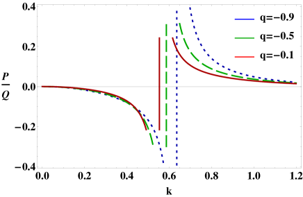
Figure 5: The variation of $P/Q$ with $k$ for different values of $q$ when $\lambda_{1}=0.007$, $\lambda_{2}=1.2$, $\lambda_{3}=0.07$, $\lambda_{4}=1.8$, $\lambda_{5}=1.5$, $\lambda_{6}=1.7$, and $\omega\equiv\omega_{f}$.

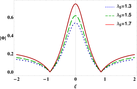
Figure 6: The variation of $|\Phi|$ with $\xi$ for different values of $\lambda_{5}$ when $\lambda_{1}=0.007$, $\lambda_{2}=1.2$, $\lambda_{3}=0.07$, $\lambda_{4}=1.8$, $\lambda_{6}=1.7$, $\tau=0$, $k=0.4$, and $\omega\equiv\omega_{f}$.

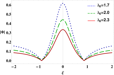
Figure 7: The variation of $|\Phi|$ with $\xi$ for different values of $\lambda_{6}$ when $\lambda_{1}=0.007$, $\lambda_{2}=1.2$, $\lambda_{3}=0.07$, $\lambda_{4}=1.8$, $\lambda_{5}=1.5$, $\tau=0$, $k=0.4$, and $\omega\equiv\omega_{f}$.

4 Stability of IAWs

The propagation of IAWs is modulationaly stable when $P$ and $Q$ have opposite sign (i.e., $P/Q<0$), and is modulationally unstable when both $P$ and $Q$ have same sign (i.e., $P/Q>0$). The point at which the transition of $P/Q$ curve intersect with the $k$-axis in the “$P/Q$ versus $k$” graph is known as threshold or critical wave number $k~{}(=k_{c})$. Under consideration of fast and slow IA modes, we have depicted the $P/Q$ versus $k$ curve for different values of $\lambda_{2}$ in Figs. 1 and 2, respectively, and it can be seen from these two figures that (a) both stable and unstable parametric regimes are allowed by the plasma system; (b) the $k_{c}$ increases (decreases) with increasing in the value of the negatively (positively) charged ion mass for a fixed value of their charge states; (c) the stable parametric regime increases (decreases) with positive (negative) ion charge state when their masses remain constant.

The effect of electron number density on the stability condition of IAWs can be understood by plotting $P/Q$ with $k$ for different values of $\lambda_{4}$ in Fig. 3. It is easy to demonstrate from this figure that the stable (unstable) parametric regime of IAWs increases (decreases) with the increase in the value of the equilibrium electron number density. The impact of sub-extensivity and super-extensivity of electrons on the stability condition of IAWs can be seen in Figs. 4 and 5, respectively. It is obvious from these two figures that the sub-extensive property of the electrons allows the IAWs to be stable for large wave number while the super-extensive property of the electrons allows the IAWs to be stable for small wave number.

5 Rogue Waves

The first-order rogue wave solution of the NLSE can be written as [28]

$$\Phi(\xi,\tau)=\sqrt{\frac{2P}{Q}}\Big{[}\frac{4+16i\tau P}{1+4\xi^{2}+16\tau^{2}P^{2}}-1\Big{]}\mbox{exp}(2i\tau P).\$$ (31)

It is worthy to mention that the first-order rogue wave solution of the NLSE indicates that a considerable amount of IAWs energy is condensed into a very small domain in DPP. The effect of the number density and charge state of both positively and negatively charged ions on the amplitude and width of the IARWs can be observed from Fig. 6. It is noted that an increase in the number density of positive (negative) ions tend to enhance (decrease) both the amplitude and width of the IARWs in the modulationally unstable parametric regime ($P/Q>0$) for a constant value of positive and negative ions charge state. The physics of this result is that an increase in the value of positive (negative) ion number density tend to increase (decrease) the nonlinearity as well as amplitude and width of the IARWs. The nature of IARWs may also be affected by the electron and positron temperature which can be observed in Fig. 7. This figure reveals that an increase in the value of the electron (positron) temperature would make the amplitude and width of the IARWs associated with IAWs smaller (taller). The physics behind this result is that the nonlinearity of the plasma medium as well as height and width of the IARWs decreases (increases) with electron (positron) temperature.

6 Conclusion

We have scrutinized the MI of IAWs and associated IARWs in a four-component DPP having inertial positive and negative ions and inertialess non-extensive electrons and iso-thermal positrons by deriving a standard NLSE. It is noted that all of the plasma components in a DPP medium play a vigorous role in the stability criteria of the IAWs. However, the essence of our findings can be summarized as follows:

1. Under consideration of fast and slow mode, both stable and unstable parametric regimes of IAWs can be observed.

2. The sub-extensive property of the electrons allows the IAWs to be stable for large wave number while the super-extensive property of the electrons allows the IAWs to be stable for small wave number.

3. An increase in the value of positive (negative) ion number density tend to increase (decrease) the nonlinearity as well as amplitude and width of the IARWs.

4. The nonlinearity of the plasma medium as well as height and width of the IARWs decreases (increases) with electron (positron) temperature.

The implications of our present investigation will be useful in understanding the process of MI of IAWs and associated IARWs in both laboratory plasma [viz., processing reactors [6], semiconductor industry [7], neutral beam sources [5], fullerene ($C^{+}_{60},C^{-}_{60}$) [13], and in intense laser fields [8]] and astrophysical environments [viz., Van Allen radiation belt and near the polar cap of fast rotation neutron stars [1], solar atmosphere [2], D-region ($H^{+},O_{2}^{-}$) and F-region ($H^{+},H^{-}$) of the earths’s ionosphere [3], upper region of Titan’s atmosphere [4], etc.].

References

• [1] A.P. Lightman, Astrophys. J. 253 (1982) 842.
• [2] E. Tandberg-Hansen and A.G. Emsile, The Physics of Solar Flares, Cambridge University Press, Cambridge, 1988.
• [3] S.A. Elwakil, et al., Phys. Plasmas 17 (2010) 052301.
• [4] S.K. El-Labany, et al., Astrophys. Space Sci. 338 (2012) 3.
• [5] M. Bacal and G.W. Hamilton, Phys. Rev. Lett. 42 (1979) 1538.
• [6] R.A. Gottscho and C.E. Gaebe, IEEE Trans. Plasma Sci. 14 (1986) 92.
• [7] P.K. Shukla, et al., Phys. Rep. 138 (1986) 1.
• [8] V. Berezhiani, et al., Phys. Rev. 46 (1992) 6608.
• [9] W. Oohara and R. Hatakeyama, Phys. Rev. Lett. 91 (2003) 205005.
• [10] P. Helander, D.J. Ward, Phys. Rev. Lett. 90 (2003) 135004.
• [11] A. Esfandyari-Kalejahi, et al., Phys. Plasmas 13 (2006) 122310.
• [12] U.M. Abdelsalam, et al., Phys. Letters A 372 (2008) 4057.
• [13] R. Sabry, Phys. Plasmas 15 (2008) 092101.
• [14] D.T. Young, et al., Science 307 (2005) 1262.
• [15] R. Lundin, et al., Nature 341 (1989) 609.
• [16] A. Renyi, Acta Math. Acad. Sci. Hung. 6 (1955) 285.
• [17] C. Tsallis, J. Stat. Phys. 52 (1988) 479.
• [18] Y.Y. Wang, et al., Phys. Lett. A 377 (2013) 2097.
• [19] Shalini, et al., Phys. Plasmas 22 (2015) 092124.
• [20] M. Tribeche, et al., Phys. Plasmas 17 (2010) 042114.
• [21] M.G. Hafez and M.R. Talukder, Astrophys. Space Sci. 359 (2015) 27.
• [22] S.K. Paul, et al., Pramana-J Phys 94 (2020) 58.
• [23] N.A. Chowdhury, et al., Phys. plasmas 24 (2017) 113701.
• [24] M.H. Rahman, et al., Chinese J. Phys. 56 (2018) 2061.
• [25] M.H. Rahman, et al., Phys. Plasmas 25 (2018) 102118.
• [26] N.A. Chowdhury, et al., Vacuum 147 (2018) 31.
• [27] N.A. Chowdhury, et al., Contrib. Plasma Phys. 58 (2018) 870.
• [28] N. Akhmediev, et al., Phys. Rev. E 80 (2009) 026601.
• [29] D. Kedziora, et al., Phys. rev. E 84 (2011) 056611.
• [30] M.N. Haque, et al., Plasma Phys. Reports 45 (2019) 1026.
• [31] M.N. Haque, et al., Contribution to Plasma Phys. 59 (2019) e201900049.
• [32] A.S. Bains, et al., Phys. of Plasmas 18 (2011) 022108.
• [33] O. Bouzit, et al., Phys. of Plasmas 22 (2015) 084506.
• [34] P. Eslami, et al., Phys. of Plasmas 18 (2011) 102313.
• [35] S. Jahan, et al., Commun. Theor. Phys. 71 (2019) 327.
• [36] P.K. Shukla and A.A. Mamun, Introduction to Dusty Plasma Physics, Institute of Physics, Bristol, 2002.
• [37] N.A. Chowdhury, et al., Plasma Phys. Report 45 (2019) 457.
• [38] N.A. Chowdhury, et al., Chaos 27 (2017) 093105.
• [39] N. Ahmed, et al., Chaos 28 (2018) 123107.
• [40] R.K. Shikha, et al., Eur. Phys. J. D 73 (2019) 177.
• [41] S. Jahan, et al., Plasma Phys. Rep. 46 (2020) 90.
• [42] M. Hassan, et al., Commun. Theor. Phys. 71 (2019) 1017.