Benchmarking the ab initio hydrogen equation of state for the interior structure of Jupiter

Abstract

Context. As Juno is presently measuring Jupiter’s gravitational moments to unprecedented accuracy, models for the interior structure of the planet are putted to the test. While equations of state based on first principles or ab initio simulations have been available and used for the two most abundant elements constituting the envelope, hydrogen and helium, significant discrepancies remain regarding the predictions of the inner structure of Jupiter. The differences are severe enough to clutter the analysis of Juno’s data and even cast doubts on the usefulness of these computationally expensive EOSs for the modeling of the interior of Jupiter and exoplanets at large

Aims. Using our newly developed equations of state for hydrogen and helium, we asses the ab initio equations of state currently available and establish their efficiency at predicting the interior structure of Jupiter in a two-layers model. We paid particular attention to the calculation of the total entropy for hydrogen that is required to calculate the convective H-He envelope but is a derived quantity from ab initio simulations.

Methods. The ab initio equations of state used in this work are based on a parameterization of the ab initio simulation points using a functional form of the Helmholtz free energy. It extends on our previous work recently published. Compared to previous ab initio equations of state available, this latter approach provides an independent mean of calculating the entropy that was recently pointed out as deficient in some ab initio results.

Results. By adjusting our free energy parameterization to reproduce previous ab initio EOS behavior, we identify the source of the disagreement previously reported for the interior structure of Jupiter. We further point to area where care should be taken when building EOS for the modeling of giant planets. This concerns the interpolation between the ab initio results and the physical models used to cover the low density range as well as the interpolation of the ab initio simulation results at high densities. This sensitivity falls well within the uncertainties of the ab initio simulations. This suggests that hydrogen EOS should be carefully benchmarked using a simple planetary model before being used in the more advanced planetary models needed to interpret the Juno data. We finally provide an updated version of our ab initio hydrogen EOS recently published.

1 Introduction

With the Juno spacecraft currently orbiting Jupiter, there is now a unique opportunity to constrain the planet inner structure using high-precision measurements of the gravitational field (Folkner et al., 2017; Bolton et al., 2017). With the first orbits now completed and analyzed, several remarkable results are already reported. This includes the magnetic field properties of the planet, the depth of the atmospheric jet-stream estimated to extend $3000\leavevmode\nobreak\$km below the surface (Guillot et al., 2018), and the suggestion that the core of the planet may be eroded and probably extending significantly outward in the envelope (Wahl et al., 2017). This latter result is potentially important to validate the core accretion scenario (Pollack et al., 1996), the formation model, and the time evolution of giant planets at large. It remains, however, cluttered by significant uncertainties regarding the predictions of the planet inner structure using various equations of state (EOS).

From the mid-90’s, interior models of Jupiter mostly relied on the benchmark EOSs of Saumon et al. (1995) (SCVH). These EOSs provided the first comprehensive description of hydrogen and helium properties in the entire regime relevant to giant planets (Guillot, 1999). These equations of state rest on a chemical description of the dense plasma and are obtained by minimizing the Helmholtz free energy of the system represented as a collection of atoms, molecules, ions, and electrons. This physically based model provides an estimation of the gradual dissociation and ionization of the hydrogen molecules taking place as the density increases along Jupiter’s interior. Among its most notable features, it predicted that dissociation of hydrogen is a first order transition that occurs within Jupiter. This phase transition justifies a three layers model for Jupiter’s interior consisting of a H-He envelope where hydrogen is neutral, an inner envelope where hydrogen turns metallic, and a solid core made of a mixture of water and silicates (Stevenson & Salpeter, 1977; Stevenson, 1982). This core is assumed to correspond to the primordial planetary embryo around which hydrogen and helium were accreted in the planetary nebula during the formation of the planet (Guillot, 1999; Pollack et al., 1996). This understanding of the interior of Jupiter was completed by considering de-mixing of the hydrogen-helium mixture in the metallic envelope to account for the measurement of a sub-solar abundance of helium in the atmosphere measured by the Galileo probe (von Zahn et al., 1998; Guillot, 1999). Demixing is also a convincing explanation of the strong depletion in neon observed by Galileo, as neon is more soluble in helium than in hydrogen (Wilson & Militzer, 2010). As mentioned earlier, the recent measurements by Juno support the existence of a diffuse core, blurring somewhat the three-layer pictures (Wahl et al., 2017). This is, however, beyond the scope of the present paper that mainly focuses on describing the H-He envelope and specifically on benchmarking the hydrogen EOS used.

These predictions of Jupiter’s inner structure based on the SCVH EOS (Saumon et al., 1995) were putted into question in the early-2000s by shock measurements of hydrogen up to a few Mbars. These measurements indicated that along the principal Hugoniot, the dissociation and metalization of hydrogen do not coincide with a first order transition in the regime relevant to giant planet interior but happen rather continuously as pressure and temperature increase (Collins et al., 1998; Knudson et al., 2001). It further showed that hydrogen is not as compressible as predicted by the SCVH EOS. These findings immediately cast shadows on the resulting model of Jupiter’s interior structure and triggered intense activities on both the experimental and theoretical sides, mostly focusing on the rate of dissociation of molecular hydrogen at planetary conditions (Saumon & Guillot, 2005).

This lead to a new generation of EOS for hydrogen and helium based on density functional theory (DFT) (Lenosky et al., 1997; Militzer & Ceperley, 2000; Desjarlais, 2003; Holst et al., 2008; Caillabet et al., 2011; Hu et al., 2011; Becker et al., 2014; Militzer & Hubbard, 2013; Miguel et al., 2016; Chabrier et al., 2019). As demonstrated by their success at describing all the experimental data obtained so far, these ab initio EOSs provide a description of the ionization and dissociation processes occurring along the principal shock Hugoniot and Jupiter’s adiabat without adjustable parameters. Despite this now undisputed ability at providing an improved description of hydrogen and helium properties at planetary conditions (Knudson et al., 2018), the situation for the interior of Jupiter still remains cluttered. At the moment two different ab initio EOSs published in the past ten years for the hydrogen-helium mixture are leading to significantly different predictions for the interior of Jupiter. The situation was recently summarized by Miguel et al. (2016). These two ab initio EOSs are leading to drastically different predictions regarding the size of the core, the distribution of metallic elements within the envelope as well as the temperature profile within the planet (Nettelmann et al., 2012; Militzer & Hubbard, 2013; Miguel et al., 2016). These differences are significant enough to currently challenge our ability to correctly interpret the data from the Juno mission and, ultimately, to use this improved knowledge to validate formation models of giant planets.

To resolve this issue, we recently developed equations of state for hydrogen, helium, and the associated H-He mixture based on density functional molecular dynamics simulations (Chabrier et al., 2019; Soubiran, 2012). Compared to previous ab initio EOSs developed by Militzer & Hubbard (2013) and Becker et al. (2014), these latest EOSs rest on an independent mean of evaluating the Helmholtz free energy. This allows us to deduce the total entropy needed to model convective envelopes, that is in agreement with both the high-pressure melting properties as well as Monte Carlo simulations (Caillabet et al., 2011). Using these EOSs, we critically compare our results with previous predictions for both the entropy and the interior structure obtained for Jupiter. Following the work of Miguel et al. (2016, 2018), we paid particular attention to the evaluation of the entropy for the case of hydrogen. To detangle the discrepancies reported so far, we adjust our free energy model to reproduce previous ab initio simulation results. Lastly, we update our initial release of the hydrogen EOS (Chabrier et al., 2019) to provide a more accurate fit of the ab initio data in the thermodynamical regime relevant to the modeling of the interior structure of Jupiter.

2 Equation of state

The study reported here is based on a new set of EOSs for hydrogen and helium covering the complete thermodynamical range relevant to astrophysical modeling (Chabrier et al., 2019; Soubiran, 2012). This density-temperature range extends significantly beyond the regime relevant to giant planets of the solar system to include hot exoplanets and brown dwarfs several times the size of Jupiter. This set of EOSs follows on the previous work of Caillabet et al. (2011) and complete ab initio simulations data using results obtained from physical models for low and extreme densities as well as for high temperatures.

Figure 1: Density-temperature diagram summarizing how the various methods are used to construct the Chabrier et al. (2019) hydrogen EOS relevant to astrophysical applications. (DFT-MD) density functional theory results of Caillabet et al. (2011), (PIMC) Path Integral Monte Carlo calculations of Militzer & Ceperley (2000), (CP) dense plasma model of Chabrier & Potekhin (1998), (SCVH) chemical model of Saumon et al. (1995). A P-T version of the diagram can be found in Chabrier et al. (2019).

Figure 1 shows how the various methods are used to build a complete hydrogen EOS covering the complete thermodynamical range of interest for astrophysical applications. For hydrogen, density functional theory based molecular dynamics simulations (DFT-MD) can be used for densities down to 0.1-0.2 g/cm³. Below this density range, the method becomes less efficient numerically. Standard DFT functionals, such as the commonly used PBE functional Perdew et al. (1997), also become less reliable. These functionals do not account for the van der Wall interactions that start to become relevant as the density decreases. The high-temperature limit of the method is more a practical one that steams from the number of Kohn-Sham orbitals that can be included in the simulation while keeping the overall simulation time tractable.

In the DFT-MD region, we used the parameterization of the ab initio results provided by Caillabet et al. (2011). This consists in adjusting two physical models on the ab initio results: a double-debye model for the solid phase and a one-component plasma model completed with a mass action law for dissociation to describe the liquid and plasma state. The input ab initio data set used to obtain this parameterization includes the DFT-MD results of Holst et al. (2008) with additional calculations performed by Caillabet et al. (2011), coupled electron-ion Monte Carlo results of Morales et al. (2010), which provides an evaluation of the Helmholtz free-energy in the liquid for temperatures ranging from $2000\leavevmode\nobreak\$K to $10000\leavevmode\nobreak\$K, and Path Integral Monte Carlo (PIMC) calculations of Militzer & Ceperley (2000). Further comparisons with more recent PIMC calculations (Hu et al., 2011) can be found in Chabrier et al. (2019).

Figure 1 shows that for hydrogen, we completed the dataset of Caillabet et al. (2011) with results of the dense plasma model (CP) (Chabrier & Potekhin, 1998) for densities above $5\leavevmode\nobreak\$g/cm³ and for temperatures above $10\leavevmode\nobreak\$eV. At low densities, we used the SCVH model (Saumon et al., 1995) to extend the ab initio data set. The helium EOS used in the present work follows the same approach with the ab initio data set based on DFT-MD simulations parameterized using a one-component plasma model and completed by both SCVH and CP results at respectively low and high densities and CP results at high temperatures. Further details on the helium EOS can be found in Soubiran (2012) and has been discussed at length in Chabrier et al. (2019). The challenge of building the overall EOS rests in assuring a smooth transition for the pressure, internal energy, and entropy as well as their derivative with respect to density and temperature. This complete set is needed for the calculation of the planetary interior structure. Figure 1 indicates that for Jupiter, the transition that requires careful monitoring is between the low density SCVH results and the ab initio ones. This transition between the two sets of calculations can be monitored by considering the principal Hugoniot.

Figure 2: Comparison between the experimental data and the various theoretical predictions for the hydrogen principal Hugoniot. The initial state is taken as $\rho_{0}$=0.085g/cm$3$ and $T=20$K. EOS-0.2 and EOS-0.8 are principal Hugoniot obtained with an interpolation range between the SCVH and ab initio data extending from $0.05\leavevmode\nobreak\$g/cm³ to, respectively, $0.2\leavevmode\nobreak\$g/cm³ and $0.8\leavevmode\nobreak\$g/cm³. The former corresponds to the Chabrier et al. (2019) EOS and is thus labeled CMS19-EOS-0.2 in the figure.

In figure 2, we compare the various theoretical predictions with the latest experimental data for the principal Hugoniot of hydrogen (Knudson et al., 2004, 2018). We first notice that the latest analysis of the shock Hugoniot data by Knudson et al. (2018) significantly reduced the error bars. It further indicates a maximum compressibility of $\rho_{1}/\rho_{0}=4.534$, which is slightly higher than previously reported (Knudson et al., 2004). When compared to the theoretical predictions, we first see, as reported previously, that the SCVH EOS misses the experimental data significantly. We further find that the results of Miguel et al. (2016) overestimates the maximum compressibility from $50\leavevmode\nobreak\$GPa and beyond. The other predictions are slightly softer than the re-analyzed data set and stand just outside the error bars. The remaining difference in compressibility has been identified as the need for higher level functionals Knudson et al. (2018). We further notice that the EOS recently published by Chabrier et al. (2019), noted CMS19 from now on, agrees nicely with this revised version of the experimental data. As expected, it is in agreement with the ab initio data (Caillabet et al., 2011) used to build it.

This revision of the experimental data has a noticeable impact for the modeling of the inner structure of Jupiter. The principal Hugoniot represents the density-temperature conditions at the edge of the interpolation region between the ab initio data and the SCVH results. Reducing the error bars on the Hugoniot measurements adds a stronger constrain on the interpolation procedure in a density region where the two data sets do not coincide for either the internal energy or the entropy. The original shock data (Knudson et al., 2004) allowed for a looser interpolation extending on a density region between $\rho=0.05$ and $0.8$g/cm³. Figure 2 shows that this leads to a principal Hugoniot, EOS-0.8, with a maximum compressibility reduced and compatible with the original shock data, the predictions of Hu et al. (2011), and Kerley (2013) (not shown in figure 2). The re-analyzed shock data lead to a reduction of the density range over which the interpolation between the SCVH and the ab initio data is performed, between $\rho=0.05$ and $0.2$g/cm³ (labeled as CMS-19-EOS-0.2 in figure 2).

Figure 3: Comparison between the (a) pressure normalized to the density and (b) internal energy as given by various EOS for hydrogen. Same legend as in figure 2, MH-SCVH stands for the Militzer & Hubbard (2013) EOS as calculated by Miguel et al. (2016).

In figure 3, we compare the pressure and internal energy for hydrogen as given by our recently published EOS, CMS-EOS-0.2, with the latest EOS of Becker et al. (2014), the standard SCVH EOS (Saumon et al., 1995) and the Militzer & Hubbard (2013) EOS as calculated by Miguel et al. (2016), MH-SCVH. We see that differences between the SCVH result and all the ab initio results are clearly visible for both the pressure and internal energy at densities above $0.1\leavevmode\nobreak\$g/cm³. This has been previously documented by several authors.

Figure 3 also shows that the overall agreement between the various ab initio results is, at first glance, rather satisfactory with some differences above 0.1g/cm³. As pointed out above, this density range corresponds to the interpolation region between the SCVH result and the ab initio data for our newly developed EOS (Chabrier et al., 2019), the EOS of Becker et al. (2014), as well as the one from Miguel et al. (2016). We point out here that Miguel et al. (2016) extracted an EOS for pure hydrogen from the H-He EOS of Militzer & Hubbard (2013) that includes the non-ideal contribution to the entropy of mixing. They further used the He SCVH EOS that differs from the ab initio results (Soubiran, 2012). Figure 3-a, where we display the pressure normalized to the density, shows that the interpolation appears rather consistent between the various EOSs when considering the pressure. In contrast, figure 3-b indicates noticeable differences in the transition region for the internal energy and for all the temperatures relevant to giant planets. The behavior of the $2000$ and $5000\leavevmode\nobreak\$K isotherms obtained with the EOS-0.8 and Becker et al. (2014) EOS suggests that this is a delicate domain. Miguel et al. (2016) noticed this behavior for the internal energy and speculated that it propagates to the evaluation of the entropy. We confirm this result here and confirm that it may explain some of the differences in the temperature profile of Jupiter obtained using various ab initio EOSs.

Figure 4: Comparison between the initial ab initio simulation points of Caillabet et al. (2011) and the various ab initio EOS available at high-density.

To further compare the various ab initio EOSs available for the modeling of Jupiter, we show in figure 4 the high-density behavior along three isotherms particularly relevant for the interior structure of Jupiter. This density-temperature regime corresponds to the planet deep envelope and close to the core-envelope boundary where significant differences have been reported between the various ab initio predictions. Figure 4 shows some differences at high densities between the three EOSs for all the temperatures investigated. When comparing to the raw ab initio data points, we see that the EOSs remain within 5% of the simulation result. For a temperature of $T=10000\leavevmode\nobreak\$K and a density of $\rho=4\leavevmode\nobreak\$g/cm³, the original Caillabet et al. (2011) fit is 2% lower than the ab initio data while both the Miguel et al. (2016) and Becker et al. (2014) are 4% higher. This difference worsen as temperature increases. At $T=20000\leavevmode\nobreak\$K and for the same density range, the difference in pressure between the Becker et al. (2014), Miguel et al. (2016), and Caillabet et al. (2011) reaches 7%. While this stays within the prescribed boundary for a fit adjusted over a broad density-temperature range, this difference is significant enough to require attention when considering the interior structure of Jupiter. We recall here that the Chabrier et al. (2019) EOS is based on the Caillabet et al. (2011) parameterization.

We further point out that the ab initio simulation points themselves have some uncertainty associated to them. Various simulation parameters such as the number of particles used in the simulation cell, the plane wave cut-off, the functional used, as well as the fluctuation naturally occurring within the simulation all bring a combined uncertainty of a few percents in the final pressure. In this context, a difference of a few percents between the different EOS based on ab initio results can be expected. While this likely explains the difference between our EOS (Chabrier et al., 2019) and the result of Becker et al. (2014), we also mention that the hydrogen EOS extracted by Miguel et al. (2016) from the H-He of Militzer & Hubbard (2013) adds an additional uncertainty by using the SCVH He EOS and by neglecting the non-ideal mixing contribution accounted for in the Militzer & Hubbard (2013) EOS. The former probably explains the difference we see here for the pressure between the hydrogen EOS extracted by Miguel et al. (2016) and the ab initio simulation points.

To test how this uncertainty propagate for the inner structure of Jupiter, we adjusted the parameterization provided by Caillabet et al. (2011) and used in Chabrier et al. (2019) to reproduce precisely the ab initio results and the pressures obtained by the two other ab initio EOSs. This is obtained by writing $d_{c}(\rho)=d_{0}\rho$ for $\rho\geq 0.419$ and varying the $d_{0}$ parameter to a value of respectively, $d_{0}=0.0326858$, $0.123$, and $0.223$. The first value corresponds to the initial parameterization of Caillabet et al. (2011) used in Chabrier et al. (2019) and Debras & Chabrier (2019), the second matches exactly the ab initio results, while the latest value reproduces the Becker et al. (2014) behavior at high densities.

Figure 5: Variation of the hydrogen entropy as a function of density for isotherms relevant to Jupiter modeling. (a) Comparison between the various ab initio predictions and the coupled electron-ion Monte Carlo result (Morales et al., 2010). (b) Comparison between the CMS-EOS-0.2 $d_{0}=0.0326858$) EOS for hydrogen, with results considering interpolation in a large density range, EOS-0.8 $d_{0}=0.0326858$, or adjusting the high pressure behavior, EOS-0.2 $d_{0}=0.132$, and with the SCVH predictions and another well used physically based EOS (Kerley, 2013).

To address the issue of the evaluation of the entropy pointed out by Miguel et al. (2016), we show in figure 5 the various ab initio predictions for isotherms representative of the interior of Jupiter. The labeling follows the one given by Miguel et al. (2016) where the entropy deduced from the EOS of Becker et al. (2014) and corrected for the energy are labeled respectively eos3b and eos3c. The entropy deduced from the H-He EOS of Militzer & Hubbard (2013) is labeled MH-SCVH. We see in figure 5-a that the predictions are overall rather consistent and in rather good agreement with the coupled electron-ion Monte Carlo calculations of Morales et al. (2010). The latter is considered as a benchmark result for the entropy. As expected, the largest differences are seen in the interpolation region for densities between $\rho=0.1\leavevmode\nobreak\$g/cm³ and $\rho=0.8\leavevmode\nobreak\$g/cm³. These differences reflect the variation that was observed for the principal Hugoniot predictions shown in figure 2. We also note that once corrected (Miguel et al., 2018), the high-temperature behavior initially noticed for the entropy deduced from the EOS of Becker et al. (2014) using thermodynamics relations tends to disappear. The results shown in figure 5 suggest that the estimation of the entropy is rather consistent between the various models. The evaluation of the entropy itself is not likely the direct cause of the differences that are reported in the predictions for the interior of Jupiter.

This is confirmed in figure 5-b, where we compare the predictions of our EOS (Chabrier et al., 2019) with the results given by the SCVH and Kerley (Kerley, 2013) EOSs. The latter is a refined version of the SCVH EOS that takes into account the experimental Z-pinch data of Knudson et al. (2004). In the interpolation region, the difference is surprisingly only noticeable at the lowest and highest temperatures displayed. We also show in figure 5-b the effect of varying the interpolation region between the SCVH and the ab initio results from the density range extending from $0.05$ to $0.2$g/cm³ to $0.05$ to $0.8$g/cm³ while keeping $d_{0}=0.0326858$. These EOS are labeled as, respectively, CMS19-EOS-0.2 and EOS-0.8. At $T=2000\leavevmode\nobreak\$K, we see that a larger interpolation range provides a smoother transition between the SCVH and ab initio data sets. The EOS-0.8-$d_{0}=0.0326858$ result is almost indistinguishable from the SCVH result. We recall from the discussion of figure 2 that this occurs at the expense of not reproducing the re-analyzed shock data. As this also corresponds to the differences in the internal energy noticed between the various models, this tends to further suggest that the different predictions for the internal energy only impact the entropy deduced in the low-temperature region of the isentrope. It is thus not likely the origin of the difference noted for the whole adiabat of Jupiter.

We also show in figure 5-b how the entropy changes when the EOS is adjusted to reproduce the initial ab initio calculations to less than 1%; noted as EOS-0.2-$d_{0}=0.123$. We see that adjusting the pressure at high densities reproduces the variations noticed between the various ab initio predictions at high densities. This suggests that the evaluation of the entropy itself, which varies in the various methods, is probably not a cause for concerns. The variation between the various predictions is mostly a propagation of the difference noticed for the energy and pressure in the interpolation between the ab initio et SCVH results and, at higher densities, in the interpolation of the ab initio results.

3 Jupiter Inner Structure

We now turn to the predictions of the interior profile of Jupiter obtained using the various EOSs discussed in the previous section. We show in figure 6 the hydrogen-helium adiabat obtained using our recent EOS (Chabrier et al., 2019) with an helium concentration $Y_{He}=0.245$. This profile is obtained by considering the planet as constituted of an isentropic hydrogen-helium envelope with an homogeneous He concentration and a central core made of heavier elements. We used the temperature measured at $1\leavevmode\nobreak\$bar by the Galileo probe (von Zahn et al., 1998), $T_{1bar}=167\leavevmode\nobreak\$K, to fixed the entropy of the isentrope using the SCVH EOS. This model assumes that the envelope is fully convective, neglects a potentially radiative outer layer (Guillot, 1999), the effect of demixing and of the multiple molecular species detected in the atmosphere by the Galileo probe (Hubbard & Militzer, 2016). With these effects neglected, the Jupiter’s interior profiles calculated thus corresponds to the H-He isentrope.

Figure 6: Jupiter interior profiles obtained with various version of the EOS adjusted at low and high densities and an helium mass fraction $Y_{He}=0.245$. (a) Comparison with previous ab initio predictions of Militzer & Hubbard (2013), Nettelmann et al. (2012), and Chabrier et al. (2019). (b) Comparison with the predictions of Miguel et al. (2016) corrected by Miguel et al. (2018). The shaded area corresponds to the result obtained when d₀ is varied as in indicated in (a).

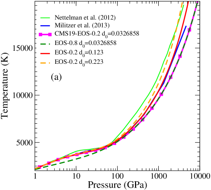
In figure 6-a, we compare our calculation for the H-He isentrope obtained for a fixed concentration of helium, $Y_{He}=0.245$, with the ab initio predictions of Militzer & Hubbard (2013) and Nettelmann et al. (2012). At low pressures, figure 6-a shows that varying the interpolation domain from 0.2 to 0.8 g/cm³, noted respectively EOS-0.2 and EOS-0.8, leads to a cooler isentrope in the $10-100\leavevmode\nobreak\$GPa range. It also removes the change of slope noticeable from $10$ to $80\leavevmode\nobreak\$GPa. This suggests that a different interpolation scheme in this density region is likely at the origin of the difference obtained for the adiabat in the $10-300\leavevmode\nobreak\$GPa range. This range also corresponds to tighter constrains from the Hugoniot data. We further see that the revision of the Hugoniot data confirms a slight variation of the slope of the adiabat of Jupiter as the pressure increase and dissociation takes place. We see that up to $100\leavevmode\nobreak\$GPa, the agreement with the prediction of Militzer & Hubbard (2013) is almost perfect while some departure is noticeable with the calculation of Nettelmann et al. (2012). The latter is consistent with the differences noticed previously in the interpolation region between the SCVH and ab initio data for, respectively, the internal energy and the entropy. We further see that these variations propagate up to a few hundreds GPa in the isentrope.

As pointed out previously (Militzer & Hubbard, 2013; Miguel et al., 2016), we see a significant departure between the previous ab initio predictions for pressures beyond $100\leavevmode\nobreak\$GPa. The differences in temperature reaches up to $3000\leavevmode\nobreak\$K at the core mantle boundary occurring at around $4000\leavevmode\nobreak\$GPa. To identify the source of this discrepancy, we show the isentropes obtained by varying the $d_{0}$ parameters in the original fit of Caillabet et al. (2011). The original value, $d_{0}=0.0326858$, and also corresponding to Chabrier et al. (2019), is varied to $d_{0}=0.123$, to match exactly the initial ab initio data, and to $d_{0}=0.223$ to match the pressure data published by Becker et al. (2014). While this variation remains within the bounds of a fit designed for a large density-temperature range, we see that the impact for the isentrope of Jupiter is rather significant. Figure 6-a shows that the intermediate value for $d_{0}$ reproduces almost exactly the isentrope calculated by Militzer & Hubbard (2013). We see that for $d_{0}=0.223$, which allows us to reproduce pressures obtained by Becker et al. (2014), the high-pressure behavior of the isentrope obtained by Nettelmann et al. (2012) is reproduced. While this isentrope is calculated with an earlier version of the hydrogen-helium equation of state (Holst et al., 2008), this comparison gives a plausible explanation for the ongoing discrepancies between these two ab initio predictions of the temperature at the core-envelope boundary.

In figure 6-b, we compare our EOSs obtained for different values of the $d_{0}$ parameter with the calculations of Miguel et al. (2016). We see that the trend noticed in figure 6-a remains the same. More specifically, we see that the isentrope deduced from the Becker et al. (2014) data, noted eos3b, is consistently higher in temperature then the other EOSs in the $0.03-1.3\leavevmode\nobreak\$g/cm³ density range. It is even close to the SCVH isentrope in this density range. In contrast to Miguel et al. (2016), we attribute this difference to the interpolation region between the SCVH and ab initio data and the internal energy obtained rather than the method used to evaluate the entropy. Beyond a density of $1.5\leavevmode\nobreak\$g/cm³, we also see that the isentrope obtained reached higher temperatures when calculated using the Becker et al. (2014) EOS. The latter clips our estimation corresponding to the highest value of $d_{0}$. In contrast, the isentrope obtained using a modified version of Militzer & Hubbard (2013) remains consistently colder. Figure 6-b shows that the mean value $d_{0}$ gives an isentrope that lays almost in between the interior profiles obtained using the Becker et al. (2014) EOS or based on the Militzer & Hubbard (2013) EOS. This result suggests that the MH13-SCVH result is not completely consistent with the initial Militzer & Hubbard (2013) EOS calculated at a fixed helium concentration. We recall here that Miguel et al. (2016) extract a pure hydrogen EOS by using the SCVH EOS for helium. As this does not coincide with the ab initio results for pure helium (Soubiran, 2012), it is not surprising that some differences remain for the isentrope. The comparison shown in figure 7 suggests that the error is on the order of $1000\leavevmode\nobreak\$K when using the EOS deduced by Miguel et al. (2016).

Figure 7: Variation of the gravitational moments, $J_{2}$ and $J_{4}$, as a function of the helium fraction, $Y_{He}$ calculated using a two-layer model, and EOSs with the two extreme values of $d_{0}$.

We show, in figure 7, the variation of the first two gravitational moments obtained using the two extreme values of $d_{0}$. These calculations are performed using the theory of figures to the third order and considering a two-layers model consisting of an H-He envelope and a core made of water. While it is now well documented that such simple model is not sufficient to calculate the gravitational moments in the Juno era (Hubbard & Militzer, 2016; Nettelmann, 2017), it enables us to quantify the uncertainty stemming from the EOS without having to consider the additional planetary model assumptions that vary from authors to authors. Following Kerley (2013), we propose that this model being used to benchmark future EOS intended for the modeling of Jupiter and the interpretation of the Juno data so as to decipher the uncertainties coming from the EOS from the ones arising from the planetary model. In figure 7, each curve represents an interior structure calculation at a fixed value of the helium concentration in the envelope while the size of the core varies. We assumed the core as made of pure water and used the ab initio EOS for dense water (Mazevet et al., 2019) to model it. Figure 7 shows that a larger amount of metallic elements is needed in the envelope to approach the measured values of the first two gravitational moments when using the EOS modified to match the Becker et al. (2014) EOS (EOS-0.2-$d_{0}=0.223$). As pointed out by Wahl et al. (2017), the size of the core does not change drastically when using the two different versions of the EOS corresponding to values of $d_{0}=0.023$ and $d_{0}=0.223$.

Figure 8: Predictions for the mass of the core and the amount of metallic elements in the envelope obtained using the 3rd order theory of figure. The published results are compared with the ones obtained by varying the $d_{0}$ parameter are shown in the figure and for a core constituted of pure water and of silicate and water.

This result is summarized in figure 8, where we compare the various predictions regarding the size of the core and the amount of metallic elements in the envelope as obtained when we vary the value of the $d_{0}$ parameter to match previous ab initio EOSs. We assume a core either made of pure water and described by the dense water ab initio EOS or a core made of water and silicates and described by the simple adiabatic pressure-density relations of Hubbard & Marley (1989). Figure 8 shows that the variation in the hydrogen ab initio EOS, embodied in the value of $d_{0}$, leads to a variation in the amount of metallic elements predicted that is comparable to the one found by Militzer & Hubbard (2013) and Nettelmann et al. (2012). Based on the comparison shown before for the EOS and the isentrope, we suggest that the remaining difference with the Nettelmann et al. (2012) comes from the remaining difference for the isentrope around $1\leavevmode\nobreak\$g/cm³ that is not completely covered by varying the $d_{0}$ parameter. We further see that this result does not depend on the nature of the core as the amount of metallic elements predicted in the envelope as $d_{0}$ is varied is similar for a pure water or a water-silicate core.

Our preferred EOS, EOS-0.2 d₀=0.123, that coincides with the ab initio simulation points to better than 1%, and corrects the original Caillabet et al. (2011) and Chabrier et al. (2019) EOS, is in rather good agreement with the predictions of Militzer & Hubbard (2013). The detailed study performed here shows that ab initio EOS for hydrogen leads to Jupiter model with a low amount of metallic elements in the envelope. It furthermore provides an explanation for the differences reported with the predictions of Nettelmann et al. (2012) that overestimates the amount of metallic elements in Jupiter’s envelope. We further point out that this difference is likely due to the uncertainty in the evaluation of the pressure either coming from the fit and/or the initial ab initio data but not due to differences in the evaluation of the entropy as suggested by Miguel et al. (2016). The latter only appears in the interpolation region between the SCVH and ab initio data and, even in this case, is a consequence of the interpolation in energy and pressure between the ab initio and SCVH data.

4 Summary

Using our newly developed equations of state for hydrogen and helium Chabrier et al. (2019), we investigate the long standing disagreement regarding the predictions of the amount of metallic elements in the envelope, the size of the core, and the temperature at the core-envelope boundary for Jupiter. We find the origin of the disagreement between the previous ab initio predictions by varying the parameters in our parameterization. We confirm the prediction of Militzer & Hubbard (2013) and point out to deficiencies in the parameterization of Becker et al. (2014) regarding the size of the core and the amount of metallic elements in the envelope. We also find that Jupiter inner structure and the associated gravitational moments are very sensitive to the evaluation of pressure and internal energy to a level that approaches the uncertainty in the ab initio simulations. It further enters the regime where the different functionals used can have some influence (Schöttler & Redmer, 2018; Mazzola et al., 2018). This is a source of concern as neither the input ab initio points or the fit developed for planetary modeling are brought to this level of accuracy. This result should be accounted for in more refined planetary models required to interpret the Juno data by using benchmarked equation of states carefully validated for all the quantities involved in planetary modeling, and particularly, the pressure, internal energy, and entropy. We suggest that a simple two-layers model provides a useful framework to benchmark future EOS. Application of this new EOS for hydrogen in a more refined planetary model as needed to interpret Juno data will be the object of further work. The benchmarked EOS for hydrogen, matching the initial ab initio points of Caillabet et al. (2011) by less than 1%, and providing an updated version of the CMS19 EOS, is provided at the following address https://luth.obspm.fr/l̃uthier/mazevet/wordpress/planets-and-exoplanets/.

Appendix A EOS and references

Name	interpolation region in $\rho$ g/cm$ˆ$3	d0	ab initio data	reference
CMS19-EOS-0.2 d0=0.0326858	0.05-0.2	0.0326858	Caillabet et al. (2011)	Chabrier et al. (2019)
EOS-0.8 d0=0.0326858	0.05-0.8	0.0326858	Caillabet et al. (2011)
EOS-0.2 d0=0.123	0.05-0.2	0.123	Caillabet et al. (2011)	This work
EOS-0.2 d0=0.223	0.05-0.2	0.223	Caillabet et al. (2011)
eos3b	-	-	Becker et al. (2014)	Miguel et al. (2018)
eos3c	-	-	Becker et al. (2014)	Miguel et al. (2016)
MH-SCVH	-	-	Militzer & Hubbard (2013)	Miguel et al. (2016)