Age-optimal Scheduling over Hybrid Channels

Abstract

We consider the problem of minimizing the age of information when a source can transmit status updates over two heterogeneous channels. Our work is motivated by recent developments in 5G mmWave technology, where transmissions may occur over an unreliable but fast (e.g., mmWave) channel or a slow reliable (e.g., sub-6GHz) channel. The unreliable channel is modeled as a time-correlated Gilbert-Elliot channel at a high rate when the channel is in the “ON” state. The reliable channel provides a deterministic but lower data rate. The scheduling strategy determines the channel to be used for transmission in each time slot, aiming to minimize the time-average age of information (AoI). The optimal scheduling problem is formulated as a Markov Decision Process (MDP), which is challenging to solve because super-modularity does not hold in a part of the state space. We address this challenge and show that a multi-dimensional threshold-type scheduling policy is optimal for minimizing the age. By exploiting the structure of the MDP and analyzing the discrete time Markov chains (DTMCs) of the threshold-type policy, we devise a low-complexity bisection algorithm to compute the optimal thresholds. We compare different scheduling policies using numerical simulations.

1 Introduction

Timely updates of the system state are of great significance in cyber-physical systems, such as vehicular networks, sensor networks, and UAV navigations. In these systems, freshly generated data is more valuable than outdated data. Age of information (AoI), or simply age, was introduced as an end-to-end application-layer metric to measure information freshness [2, 3, 4, 5, 6, 7, 8, 9, 10, 11, 12, 13, 14, 15, 16, 17, 18, 19, 20, 21, 22, 23, 24, 25]. The age at time $t$ is defined as $\Delta(t)=t-U_{t}$, where $U_{t}$ is the generation time of the freshest packet that has been received by time $t$. The difference between age and classical performance metrics of wireless networks like delay and throughput is evident even in elementary queuing systems [3]. High throughput requires frequent status updates, which would cause a long waiting time in the queue that worsens timeliness. On the other hand, delay and waiting time can be greatly reduced by decreasing the update frequency, which, however, may increase the age because the status is updated infrequently.

In future wireless networks, sub-6GHz frequency spectrum is insufficient for fulfilling the high throughput demand of emerging real-time applications such as VR/AR applications, where contents must be delivered within 5-20 ms of latency, requiring a high throughput of 400-600 Mbps [26]. To address this challenge, 5G technology utilizes high-frequency millimeter wave (mmWave) bands such as 28/38 GHz, which provide a much higher data rate than sub-6GHz [27]. Verizon and Samsung demonstrated that a throughput of nearly 4Gbps was achieved in their mmWave demo system, using a 28GHz frequency band with 800MHz bandwidth [28]. However, unlike sub-6GHz spectrum bands, mmWave channels are highly unreliable due to blocking susceptibility, strong atmospheric absorption, and low penetration. Real-world smartphone experiments have shown that even obstructions by hands could significantly degrade the mmWave throughput [29]. One solution to mitigate this effect is to let sub-6GHz coexist with mmWave to form two heterogeneous channels, so that the user equipment can offload data to sub-6GHz when mmWave communications are unfeasible [30, 31, 32, 33]. Some work has already been done based on mmWave/sub-6GHz heterogeneous networks [34, 35]. However, how to improve information freshness in such hybrid networks has remained largely unexplored.

In this study, we consider a hybrid status updating system where a source can transmit the update packets over an unreliable but fast mmWave channel or a slow reliable sub-6GHz channel. Our objective is to find a dynamic channel scheduling policy that minimizes the long-term average expected age. The main contributions of this paper are stated as follows:

• The optimal scheduling problem for minimizing the age over heterogeneous channels is formulated as a Markov Decision Process (MDP). The state transition of this MDP is complicated for two reasons: (i) the two channels have different data rates and packet transmission times, and (ii) the state of the unreliable mmWave channel is correlated over time. We prove that there exists a multi-dimensional threshold-type scheduling policy that is optimal. This optimality result holds for all possible values of the channel parameters. One of the tools for proving this result is super-modularity [36]. Because of the complicated state transitions, super-modularity holds in a part of the state space but not in the rest of the state space. This is a key difference from the scheduling problems considered earlier in prior studies, e.g., [37, 38, 39, 23, 22, 40, 10]. To conquer this challenge, we develop additional techniques to show that the optimal scheduling policy has a threshold-type structure over the entire state space, including the part of state space where super-modularity does not hold.

• The state transition of the discrete time Markov chain (DTMC) for the threshold-type scheduling policy is complicated. Nonetheless, we show that the thresholds of the optimal scheduling policy can be evaluated efficiently, by using closed-form expressions or a low-complexity bisection search algorithm. Compared with the algorithms for calculating the thresholds and optimal scheduling policies in, e.g., [37, 38, 39, 23, 22, 40, 10], our solution algorithms have much lower computational complexities.

• In the special case that the state of the unreliable mmWave channel is independent and identically distributed (i.i.d.) over time, the optimal scheduling policy is shown to possess a simpler and interesting form. Finally, numerical results are provided to validate our results by comparing with several other policies.

2 Related Works

Age of information has become a popular research topic in recent years, e.g., [2, 3, 4, 5, 6, 7, 8, 9, 10, 11, 12, 13, 14, 15, 16, 17, 18, 19, 20, 21, 22, 23, 24, 25]. A comprehensive survey of the area was recently provided in [2]. First, there has been substantial work on age performance analysis in queuing systems [3, 4, 5, 6, 8, 7]. Average age and peak age in elementary queuing systems were analyzed in [3, 4, 5]. A similar setting was considered in [6] where the inter-arrival times or service times follow a Gilbert-Elliot two-state Markov chain model. A Last-Generated, First-Served (LGFS) policy was shown (near) optimal in single-source, multi-server, and multihop networks with arbitrary packet generation and arrival process [8, 7]. These results were extended to multi-source multi-server networks in [9].

Next, there has been a significant effort in age-optimal sampling [22, 10, 11, 21, 12]. The optimal sampling policy was provided for minimizing a monotonic age function in [22, 10, 21]. Joint Sampling and scheduling in multi-source systems were analyzed in [12] where the objective problem could be decoupled into maximum age first (MAF) scheduling [9] and an optimal sampling problem. Finally, age in wireless networks has been substantially explored in [13, 14, 16, 17, 18, 19, 20]. Scheduling in a broadcast network with random arrivals was provided where Whittle index policy can achieve (near) age optimality [13]. Some other age-optimal scheduling for cellular networks were considered in [14, 16, 17, 18, 25]. A class of age-optimal scheduling policies was analyzed in the asymptotic regime when the number of sources and channels both grow to infinity [19]. An age-optimal multi-path routing strategy was introduced in [20].

However, the age-optimal scheduling problem via heterogeneous channels has been largely unexplored yet. Technical results for similar models were reported in [23, 24]. In these studies, it is assumed that the first channel is unreliable but consumes a lower cost, and the second channel has the same delay as the first channel, but depletes a higher cost. Optimal scheduling policies were derived to achieve the optimal trade-off between age performance and cost.

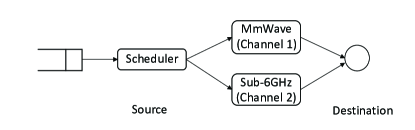
Figure 1: The system model for status updates in heterogeneous channels. The scheduler chooses mmWave (Channel 1) or sub-6GHz (Channel 2) for transmission over time.

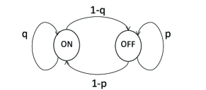
Figure 2: The Gilbert-Elliot $ON$-$OFF$ Markov model for Channel 1.

Our study is different from [23, 24] in two aspects: (i) The study in [23, 24] show the optimality of a threshold-type policy and efficiently computes the optimal threshold when the first channel is i.i.d. [23], but our work allows a Markovian channel which generalizes the i.i.d. channel model in [23]. (ii) In addition, our study assumes that the second sub-6GHz channel has a larger delay than the first mmWave which complies with the property of dual mmWave/sub-6GHz channels in real applications. These two differences between mmWave and sub-6GHz make the MDP formulation more complex than those of [23, 24]. Thus, the techniques in e.g., [37, 38, 39, 23, 22, 40, 10] that can show a nice structure of the optimal policy or solve the optimal policy with low complexity do not apply to our model.

3 System Model and Problem Formulation

3.1 System Models

Consider a single-hop network as illustrated in Fig. 1, where a source sends status update packets to the destination. We assume that time is slotted with slot index $t\in\{0,1,2...\}$. The source can generate a fresh status update packet at the beginning of each time slot. The packets can be transmitted either over the mmWave channel or over the sub-6GHz channel. The packet transmission time of the mmWave channel is $1$ time slot, whereas the packet transmission time of the sub-6GHz channel is $d$ time slots ($d\geq 2$) because of its lower data rate. The two channels have different advantages, which is the key feature of our study.

The mmWave channel, called Channel 1, follows a two-state Gilbert-Elliot model that is shown in Fig. 2. We say that Channel $1$ is $ON$ in time slot $t$, denoted by $l_{1}(t)=1$, if the packet is successfully transmitted to the destination in time slot $t$; otherwise Channel $1$ is said to be $OFF$, denoted by $l_{1}(t)=0$. If a packet is not successfully transmitted, then it is dropped, and a new status update packet is generated at the beginning of the next time slot. The self transition probability of the $ON$ state is $q$, and the self transition probability of the $OFF$ state is $p$, where $0<q<1$ and $0<p<1$. We assume that at the beginning of time slot $t$, the source knows $l_{1}(t-1)$ perfectly.

The sub-6GHz channel, called Channel 2, has a steady connection. As mentioned above, the packet transmission time of Channel 2 is $d$ time slots. Define $l_{2}(t)\in\{0,1,...,d-1\}$ as the state of Channel 2 in time slot $t$, where $l_{2}(t)$ is the remaining transmission time of the packet being sent over Channel $2$ at the beginning of time slot $t$, and $l_{2}(t)=0$ means that Channel $2$ is currently idle and ready for sending the next packet. In time slot $t$, the source has immediate knowledge about the state $l_{2}(t)$ of Channel $2$. On the other hand, because the packet transmission time of Channel 1 is 1 time slot, Channel 1 is always ready for transmission at the beginning of each time slot.

Following the application settings in [30, 31, 32, 34, 33], a packet can be transmitted using only one channel at a time, i.e., the two channels cannot be used simultaneously. The scheduler decides which channel to use for transmitting a packet at each time slot. We also assume that the scheduler can choose idle (neither channel) since it has been shown that channel idling could reduce the average age in some systems [22, 12, 10]. Hence, the scheduling decision at the beginning of time slot $t$ can be denoted by $u(t)\in\{1,2,{none}\}$. The action $u(t)=1$ or $2$ means that the source generates a packet and assigns it to Channel $1$ or Channel $2$, respectively. The action $u(t)=none$ means that no new packet is assigned to any channel at time slot $t$. Hence, u(t) = $none$ can occur if (i) a packet is was assigned to Channel 2 earlier and has not completed its transmission, i.e., $l_{2}(t)\in\{1,2,\ldots,d-1\}$ such that no packet can be assigned for transmission, or (ii) $l_{2}(t)=0$, but both channels are kept idle on purpose.

The age of information (AoI) $\Delta(t)$ is the time difference between the current time slot $t$ and the generation time of the freshest delivered packet [3]. By this definition, when a packet is delivered, the age drops to the transmission time duration of the delivered packet. Specifically, if Channel 1 is selected in time slot $t$ and Channel 1 is $ON$, then the age drops to $1$ at time slot $t+1$. If the remaining service time of Channel 2 at time slot $t$ is 1, then age drops to $d$ at time slot $t+1$. When there is no packet delivery at time slot $t$, the age increases by one in each time slot. Hence, the time-evolution of the age is given by

$$\Delta(t+1)=\left\{\begin{array}[]{lll}1&\text{if }u(t)=1\text{ and }l_{1}(t)=1,\\ d&\text{if }l_{2}(t)=1,\\ \Delta(t)+1&\text{Otherwise.}\end{array}\right.$$ (1)

3.2 Problem Formulations

Table I: Value of State Transition Probability

$P_{\textbf{ss}^{\prime}}(u)$	Action and State Transition
$p$	$u=1,\textbf{s}=(\delta,0,0),\textbf{s}^{\prime}=(\delta+1,0,0)$
	$u=2,\textbf{s}=(\delta,0,0),\textbf{s}^{\prime}=(\delta+1,0,d-1)$
	$u=none,\textbf{s}=(\delta,0,0),\textbf{s}^{\prime}=(\delta+1,0,0)$
	$u=none,\textbf{s}=(\delta,0,l_{2}),\textbf{s}^{\prime}=(\delta+1,0,l_{2}-1),l_{2}\geq 2$
	$u=none,\textbf{s}=(\delta,0,1),\textbf{s}^{\prime}=(d,0,0)$
$1-p$	$u=1,\textbf{s}=(\delta,0,0),\textbf{s}^{\prime}=(1,1,0)$
	$u=2,\textbf{s}=(\delta,0,0),\textbf{s}^{\prime}=(\delta+1,1,d-1)$
	$u=none,\textbf{s}=(\delta,0,0),\textbf{s}^{\prime}=(\delta+1,1,0)$
	$u=none,\textbf{s}=(\delta,0,l_{2}),\textbf{s}^{\prime}=(\delta+1,1,l_{2}-1),l_{2}\geq 2$
	$u=none,\textbf{s}=(\delta,0,1),\textbf{s}^{\prime}=(d,1,0)$
$q$	$u=1,\textbf{s}=(\delta,1,0),\textbf{s}^{\prime}=(1,1,0)$
	$u=2,\textbf{s}=(\delta,1,0),\textbf{s}^{\prime}=(\delta+1,1,d-1)$
	$u=none,\textbf{s}=(\delta,1,0),\textbf{s}^{\prime}=(\delta+1,1,0)$
	$u=none,\textbf{s}=(\delta,1,l_{2}),\textbf{s}^{\prime}=(\delta+1,1,l_{2}-1),l_{2}\geq 2$
	$u=none,\textbf{s}=(\delta,1,1),\textbf{s}^{\prime}=(d,1,0)$
$1-q$	$u=1,\textbf{s}=(\delta,1,0),\textbf{s}^{\prime}=(\delta+1,0,0)$
	$u=2,\textbf{s}=(\delta,1,0),\textbf{s}^{\prime}=(\delta+1,0,d-1)$
	$u=none,\textbf{s}=(\delta,1,0),\textbf{s}^{\prime}=(\delta+1,0,0)$
	$u=none,\textbf{s}=(\delta,1,l_{2}),\textbf{s}^{\prime}=(\delta+1,0,l_{2}-1),l_{2}\geq 2$
	$u=none,\textbf{s}=(\delta,1,1),\textbf{s}^{\prime}=(d,0,0)$
$0$	Otherwise

We use ${\pi}=\{u(0),u(1)...\}$ to denote a scheduling policy. A scheduling policy is said to be admissible if (i) $u(t)=none$ whenever $l_{2}(t)\geq 1$ and (ii) $u(t)$ is determined by the current and history information that is available at the scheduler. Let $\Delta_{{\pi}}(t)$ denote the AoI induced by policy $\pi$. The expected time-average age of policy ${\pi}$ is

$$\limsup_{T\rightarrow\infty}\frac{1}{T}\sum_{t=1}^{T}\mathbb{E}[\Delta_{\pi}(t)].$$

Our objective in this paper is to solve the following optimal scheduling problem for minimizing the expected time-average age:

$$\bar{\Delta}_{\text{opt}}=\inf_{\pi\in\Pi}\limsup_{T\rightarrow\infty}\frac{1}{T}\sum_{t=1}^{T}\mathbb{E}[\Delta_{\pi}(t)],$$ (2)

where ${\Pi}$ is the set of all admissible policies. Problem (2) can be equivalently expressed as an infinite time-horizon average-cost MDP problem [41, 38], which is illustrated below.

• Markov State: The system state in time slot $t$ is defined as

  $$\textbf{s}(t)=(\Delta(t),l_{1}(t-1),l_{2}(t)),$$ (3)

  where $\Delta(t)\in\{1,2,3,...\}$ is the AoI in time slot $t$, $l_{1}(t-1)\in\{0,1\}$ is the $ON-OFF$ state of Channel $1$ in time slot $t-1$, and $l_{2}(t)\in\{0,1,...,d-1\}$ is the remaining transmission time of Channel $2$ at the beginning of time slot $t$. Let S denote the state space which is countably infinite. The time-evolution of $\Delta(t)$ is determined by the state and action in time slot $t-1$.

• Action: As mentioned before, if Channel $2$ is busy (i.e., $l_{2}(t)>0$), the scheduler always chooses an idle action, i.e., $u(t)=none$. Otherwise, the action $u(t)\in\{1,2,{none}\}$.

• Cost function: Suppose that a decision $u(t)$ is applied at a time slot $t$, we encounter a cost $C(\textbf{s}(t),u(t))=\Delta(t)$.

• Transition probability: We use $P_{\textbf{ss}^{\prime}}(u)$ to denote the transition probability from state s to $\textbf{s}^{\prime}$ for action $u$. The value of $P_{\textbf{ss}^{\prime}}(u)$ is summarized in Table I.

  We provide an explanation of the transition probabilities $P_{\textbf{ss}^{\prime}}(u)$ in Table I. Due to the Markovian state transition properties of Channel $1$, there are four possible values of state transition probabilities: $p,1-p,q$ and $1-q$. For example, $P_{\textbf{ss}^{\prime}}(u)=p$ if both the current and previous states of Channel $1$ is $OFF$. Thus, there are two possible age state evolutions: if the remaining time slot of Channel $2$ is $1$, the age $\delta$ decreases to $d$; otherwise, the age $\delta$ increases by one time slot. The transition probabilities of other cases, i.e., $P_{\textbf{ss}^{\prime}}(u)=1-p,q$ and $1-q$ in Table I can be explained in the similar way.

4 Main Results

In this section, we show that there exists a threshold-type policy that solves Problem (2). We then provide a low-complexity algorithm to obtain the optimal policy and optimal average age.

4.1 Optimality of Threshold-type Policies

As mentioned in Section 3.2, the action space of the MDP allows $u(t)=none$ even if Channel $2$ is idle, i.e., $l_{2}(t)=0$. In the following lemma, we show that the action $u(t)=none$ can be abandoned when $l_{2}(t)=0$. Define

$$\Pi^{\prime}=\{\pi\in\Pi:u(t)\neq none,\text{ if }l_{2}(t)=0\}.$$ (4)

Lemma 1.

For any $\pi\in\Pi$, there exists a policy $\pi^{\prime}\in\Pi^{\prime}$ that is no worse than $\pi$.

Remark 1.

In [22, 12, 10], it was shown that in certain systems, the zero wait policy (transmitting immediately after the previous update has been received) might not be optimal. However, in our model, the zero wait policy is indeed optimal. The reason is that in our model, the minimum non-zero waiting time is one time slot which is the same as the delay of Channel $1$. If $l_{2}(t)=0$, it is better to choose Channel $1$ than keeping both channels idle, because, by choosing Channel $1$, fresh packets could be delivered over Channel $1$.

The proof of Lemma 1 is provided in Appendix A. By Lemma 1, the scheduler only needs to choose from the actions $u(t)\in\{1,2\}$ when $l_{2}(t)=0$. This lemma simplifies the MDP problem.

The parameters of the hybrid channels are $(p,q,d)$, where $p,q$ are the self transition probabilities of Channel $1$ and $d$ is the transmission delay of Channel $2$. For the ease of presenting our main results, we divide the possible values of channel parameters $(p,q,d)$ into four complementary regions $\textbf{B}_{1},\ldots,\textbf{B}_{4}$.

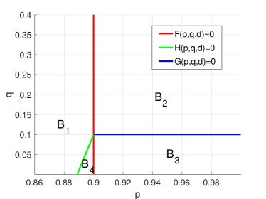
Figure 3: The Diagram of the regions $\textbf{B}_{1},\ldots,\textbf{B}_{4}$ with an example of $d=10$. In the diagram, each function $F,G,H$ divides the whole plane $((p,q)\in(0,1)\times(0,1))$ into two half-planes respectively. Each region $\textbf{B}_{1},\ldots,\textbf{B}_{4}$ is the intersection of some two half-plane areas. Since we emphasize the differences of the four regions, we provide the partial but enlarged diagram.

Definition 1.

The regions $\textbf{B}_{1},\ldots,\textbf{B}_{4}$ are defined as

$$\begin{split}\textbf{B}_{1}&=\{(p,q,d):F(p,q,d)\leq 0,H(p,q,d)\leq 0\},\\ \textbf{B}_{2}&=\{(p,q,d):F(p,q,d)>0,G(p,q,d)\leq 0\},\\ \textbf{B}_{3}&=\{(p,q,d):F(p,q,d)>0,G(p,q,d)>0\},\\ \textbf{B}_{4}&=\{(p,q,d):F(p,q,d)\leq 0,H(p,q,d)>0\},\end{split}$$ (5)

where

$$\begin{split}&F(p,q,d)=\frac{1}{1-p}-d,\\ &G(p,q,d)=1-dq,\\ &H(p,q,d)=\frac{1-q}{1-p}+1-d.\end{split}$$ (6)

Note that the inequality ${1}/(1-p)>d$ also represents a comparison between the channel delay $d$ and the average waiting time for an $ON$ channel state given that the last channel state is $OFF$. Similarly, $1-dq>0$ represents a comparison between $d$ and the average waiting time for an $ON$ channel state given that the last channel state is $ON$. Finally, $(1-q)/(1-p)+1>d$ represents a comparison between $d$ and the average waiting time of Channel $1$ under steady-state distribution of the Gilbert-Elliot model. These comparisons interpret all the boundary functions $F,G,H$ of the regions $\textbf{B}_{1}-\textbf{B}_{4}$. The four regions $\textbf{B}_{1},\ldots,\textbf{B}_{4}$ are depicted in Fig. 3, for the case that $d=10$.

Consider a stationary policy $\mu(\delta,l_{1},l_{2})$. As mentioned in Lemma 1, when $l_{2}=0$, the decision $\mu(\delta,l_{1},0)$ can be $1$ (Channel $1$) or $2$ (Channel $2$). Given the value of $l_{1}$, $\mu(\delta,l_{1},0)$ is said to be non-decreasing in the age $\delta$, if

$$\mu(\delta,l_{1},0)=\left\{\begin{array}[]{lll}1&\text{if }\leavevmode\nobreak\ \delta<\lambda;\\ 2&\text{if }\leavevmode\nobreak\ \delta\geq\lambda.\end{array}\right.$$ (7)

Conversely, $\mu(\delta,l_{1},0)$ is said to be non-increasing in the age $\delta$, if

$$\mu(\delta,l_{1},0)=\left\{\begin{array}[]{lll}2&\text{if }\leavevmode\nobreak\ \delta<\lambda;\\ 1&\text{if }\leavevmode\nobreak\ \delta\geq\lambda.\end{array}\right.$$ (8)

One can observe that scheduling policies in the form of (7) and (8) are both with a threshold-type, where $\lambda$ is the threshold on the age $\delta$ at which the value of $\mu(\delta,l_{1},0)$ changes.

One optimal solution to Problem (2) is of a special threshold-type structure, as stated in the following theorem:

Theorem 1.

There exists an optimal solution $\mu^{*}(\delta,l_{1},0)$ to Problem (2), which satisfies the following properties:

• if $(p,q,d)\in\textbf{B}_{1}$, then $\mu^{*}(\delta,0,0)$ is non-increasing in the age $\delta$ and $\mu^{*}(\delta,1,0)$ is non-increasing in the age $\delta$;

• if $(p,q,d)\in\textbf{B}_{2}$, then $\mu^{*}(\delta,0,0)$ is non-decreasing in the age $\delta$ and $\mu^{*}(\delta,1,0)$ is non-increasing in the age $\delta$;

• if $(p,q,d)\in\textbf{B}_{3}$, then $\mu^{*}(\delta,0,0)$ is non-decreasing in the age $\delta$ and $\mu^{*}(\delta,1,0)$ is non-decreasing in the age $\delta$;

• if $(p,q,d)\in\textbf{B}_{4}$, then $\mu^{*}(\delta,0,0)$ is non-increasing in the age $\delta$ and $\mu^{*}(\delta,1,0)$ is non-decreasing in the age $\delta$.

Proof.

See Section 7.2 for the proof. ∎

As is shown in Theorem 1, for all possible parameters $(p,q,d)$ of the two channels, the optimal action $\mu^{*}(\delta,l_{1},0)$ of channel selection is a monotonic function of the age $\delta$. Whether $\mu^{*}(\delta,l_{1},0)$ is non-decreasing or non-increasing in $\delta$ depends on the region of the channel parameters $(p,q,d)$ and the previous state $l_{1}$ of Channel 1.

The study in [23] assumed that the first channel is unreliable and consumes a lower cost, and the second channel the same delay as the first channel but a higher cost. They studied the scheduling policy for optimizing the trade-off between age and cost. The optimal scheduling policy in Theorem 1 is quite different from that in [23]: The study in [23] assumes the first channel to be i.i.d., but our result allows a Markovian Channel $1$, which is a generalization of the i.i.d. case. Observe that in [23], the first channel is no better than the second channel with regard to delay and reliability. However, in our study, the two channels (i.e., Channel $1$ and $2$) have their own advantages in delay and reliability. Therefore, the optimal solution in our study is non-decreasing in age for some values of $(p,q,d)$ and non-increasing in age for the remaining values of $(p,q,d)$. In conclusion, our study allows for general channel parameters $(p,q,d)$ and our optimal decision $\mu^{*}(\delta,l_{1},0)$ is non-increasing in age or non-decreasing in age depending on the choices of channel parameters.

4.1.1 Insights Behind the Regions $\textbf{B}_{1}-\textbf{B}_{4}$

The regions $\textbf{B}_{1}-\textbf{B}_{4}$ were introduced in Theorem 1 for proving that the action value function $Q(\textbf{s},u)$ is super-modular or sub-modular, where $\textbf{s}=(\delta,l_{1},0)$ denotes the state of the MDP and $u$ is the action. For example, in the case of $l_{1}=0$, if ${1}/(1-p)>d$ and ${1}/{q}\leq d$ (i.e., $(p,q,d)\in\textbf{B}_{2}$), Lemma 9 in Section 7.2 showed that $Q(\delta,0,0,u)$ is sub-modular in $(\delta,u)$ (in the discounted case). As a result, the optimal action $\mu^{*}(\delta,0,0)$ is increasing in $\delta$.

However, in the case $l_{1}=1$ of Theorem 1, there are additional technical challenges: For example, if $(p,q,d)\in\textbf{B}_{2}$, $Q(\delta,1,0,u)$ is neither super-modular nor sub-modular. A new method was developed in Lemma 10 in Section 7.2 to conquer this challenge. Technically, super-/sub-modularity is a sufficient but not necessary condition for the monotonicity of $\mu^{*}(\delta,l_{1},0)$. When neither super-modularity nor sub-modularity holds, we are able to show that the optimal decision $\mu^{*}(\delta,l_{1},0)$ does not change with $\delta$. By this, we proved the monotonicity of $\mu^{*}(\delta,l_{1},0)$ for all values of $\delta$ and $l_{1}$, without requiring $Q(\textbf{s},u)$ to be super-modular or sub-modular over the entire state space $\textbf{s}\in\textbf{S}$.

The following is one of the key technical contributions of the paper: we proved that the optimal action $\mu^{*}(\delta,l_{1},0)$ is monotonic in $\delta$ even if super-/sub-modularity does not hold. This is a key difference from prior studies, e.g., [37, 38, 39, 23, 22, 10], where super-modularity (or sub-modularity) holds for the entire state space.

4.2 Optimal Scheduling Policy

In Theorem 1, we have characterized the threshold structure for an optimal policy in region $\textbf{B}_{1},\ldots,\textbf{B}_{4}$. A threshold-type policy is fully identified by its thresholds $\lambda_{0},\lambda_{1}$, where $\lambda_{0}$ is the threshold given that the previous state of Channel $1$ is $OFF$ (i.e., $l_{1}=0$) and $\lambda_{1}$ is the threshold given that the previous state of Channel $1$ is $ON$ (i.e., $l_{1}=1$). Thus, for a given region $\textbf{B}_{i}$ $(i=1,\ldots,4)$, the MDP problem (2) reduces to

$$\bar{\Delta}_{\text{opt}}=\min_{\lambda_{0}\in\mathbb{N}^{+},\lambda_{1}\in\mathbb{N}^{+}}\bar{\Delta}_{i}(\lambda_{0},\lambda_{1}),$$ (9)

where $\bar{\Delta}_{i}(\lambda_{0},\lambda_{1})$ is the long term average cost of the threshold-type policy such that: $(1)$ the threshold (monotone) structure is determined by Theorem 1 and $\textbf{B}_{i}$; $(2)$ the thresholds are $\lambda_{0},\lambda_{1}$. Note that a threshold type policy is stationary and thus can be modeled as a discrete-time Markov chain (DTMC). Then, (9) can be solved by deriving the steady-state distribution of the DTMC.

We use $\lambda_{0}^{*}$ and $\lambda_{1}^{*}$ to denote the thresholds of $\mu^{*}(\delta,0,0)$ and $\mu^{*}(\delta,1,0)$, respectively. In this section, we provide the optimal scheduling policy and the thresholds.

4.2.1 Optimal Scheduling Policy for $(p,q,d)\in\textbf{B}_{1}$

Theorem 2.

If $(p,q,d)\in\textbf{B}_{1}$, then an optimal scheduling policy is

$$\mu^{*}(\delta,0,0)=1,\delta\geq 1;$$ (10)

$$\mu^{*}(\delta,1,0)=1,\delta\geq 1.$$ (11)

In this case, the optimal objective value of (2) is

$$\bar{\Delta}_{\text{opt}}=\frac{(1-q)(2-p)+(1-p)^{2}}{(2-q-p)(1-p)}.$$ (12)

We provide an insight to Theorem 2: As will be shown by Lemma 11 and Lemma 12 in Section 7.3, if $(p,q,d)\in\textbf{B}_{1}$, then $\mu^{*}(1,0,0)=1$ and $\mu^{*}(1,1,0)=1$. According to Theorem 1 (a), if $(p,q,d)\in\textbf{B}_{1}$, $\mu^{*}(\delta,0,0)$ and $\mu^{*}(\delta,1,0)$ are both non-increasing in $\delta$. Thus, $\mu^{*}(\delta,0,0)=1$ and $\mu^{*}(\delta,1,0)=1$ for all $\delta\geq 1$. That is, the optimal scheduler always chooses Channel $1$. The DTMC for a policy always choosing Channel $1$ is easy to analyze. We omit the derivation steps and provide

$$\bar{\Delta}_{\text{opt}}=\bar{\Delta}_{1}(1,1)=\frac{(1-q)(2-p)+(1-p)^{2}}{(2-q-p)(1-p)}.$$ (13)

This result directly implies Theorem 2.

4.2.2 Optimal Scheduling Policy for $(p,q,d)\in\textbf{B}_{2}$

While the result of case $(p,q,d)\in\textbf{B}_{1}$ is easy to describe, the result of case $(p,q,d)\in\textbf{B}_{2}$ is not. As shown by Theorem 3, the optimal decision $\mu^{*}(\delta,l_{1},0)$ is not constant in age $\delta$.

Theorem 3.

If $(p,q,d)\in\textbf{B}_{2}$, then an optimal scheduling policy is

$$\mu^{*}(\delta,0,0)=\left\{\begin{array}[]{lll}1&\text{if }\leavevmode\nobreak\ \delta<\lambda_{0}^{*};\\ 2&\text{if }\leavevmode\nobreak\ \delta\geq\lambda_{0}^{*},\end{array}\right.$$ (16)

$$\mu^{*}(\delta,1,0)=\left\{\begin{array}[]{lll}2&\text{if }\leavevmode\nobreak\ \delta<\lambda_{1}^{*};\\ 1&\text{if }\leavevmode\nobreak\ \delta\geq\lambda_{1}^{*},\end{array}\right.$$ (19)

1 Given function $h_{i}$. $l=0$, $l^{\prime}$ sufficiently large, tolerance $\epsilon$ small. The value $i\in\{1,2,3,4\}$.

2repeat

3  $\beta=\frac{1}{2}(l+l^{\prime})$

4  if $h_{i}(\beta)<0$: $l^{\prime}=\beta$. else $l=\beta$

5until $l^{\prime}-l<\epsilon$

return $\beta_{i}=\beta$

Algorithm 1 Bisection method for solving (25)

where $\lambda_{0}^{*}$ is unique, but $\lambda_{1}^{*}$ may take multiple values, given by

$$\!\!\!\!\!\left\{\begin{array}[]{lll}\lambda_{0}^{*}=s_{1}(\beta_{1}),&\lambda_{1}^{*}=1&\text{if }\leavevmode\nobreak\ \bar{\Delta}_{\text{opt}}=\beta_{1},\\ \lambda_{0}^{*}=s_{2}(\beta_{2}),&\lambda_{1}^{*}=1&\text{if }\leavevmode\nobreak\ \bar{\Delta}_{\text{opt}}=\beta_{2},\\ \lambda_{0}^{*}=1,&\lambda_{1}^{*}\in\{2,3,\ldots,d\}&\text{if }\leavevmode\nobreak\ \bar{\Delta}_{\text{opt}}=f_{0}/g_{0},\\ \lambda_{0}^{*}=1,&\lambda_{1}^{*}\in\{d+1,\ldots\}&\text{if }\leavevmode\nobreak\ \bar{\Delta}_{\text{opt}}=(3/2)d-1/2,\end{array}\right.\!\!\!\!\!$$ (20)

$\bar{\Delta}_{\text{opt}}$ is the optimal objective value of (2), determined by

$$\bar{\Delta}_{\text{opt}}=\min\Big{\{}\beta_{1},\beta_{2},\frac{f_{0}}{g_{0}},\frac{3}{2}d-\frac{1}{2}\Big{\}},$$ (21)

$s_{1}(\cdot)$, $s_{2}(\cdot)$, $\beta_{1}$, and $\beta_{2}$ are given in Definition 2 below, and

$$f_{0}=q\sum_{i=1}^{d}i+(1-q)\sum_{i=d+1}^{2d}i+\Big{(}\frac{b^{\prime}_{d}q+b_{d}}{1-b_{d}}+1\Big{)}\sum_{i=d+1}^{2d}i,$$ (22)

$$g_{0}=\frac{b^{\prime}_{d}q+b_{d}}{1-b_{d}}d+d+1,$$ (23)

$$\begin{bmatrix}b^{\prime}_{d}\\ b_{d}\end{bmatrix}=\begin{bmatrix}q&1-q\\ 1-p&p\end{bmatrix}^{d}\begin{bmatrix}0\\ 1\end{bmatrix}.$$ (24)

Proof.

See Section 7.3. ∎

In order to prove Theorem 3, we have conducted steady-state analysis of four DTMCs, each of which corresponds to one case in (20). These four DTMCs have diverse state transmission matrices and have to be analyzed separately.

For each case, the optimal thresholds $\lambda_{0}^{*}$ and $\lambda_{1}^{*}$ can be either expressed in closed-form, or computed by using a low-complexity bisection search method to compute the root of (25) given in below.

Definition 2.

The value of $\beta_{i}$ is the root of

$$\begin{split}f_{i}\big{(}s_{i}(\beta_{i})\big{)}-\beta_{i}g_{i}\big{(}s_{i}(\beta_{i})\big{)}=0,\leavevmode\nobreak\ i\in\{1,2,3,4\},\end{split}$$ (25)

where

$$s_{i}(\beta_{i})=\max\left\{\left\lceil\frac{-k_{i}(\beta_{i})}{1-d(1-p)}\right\rceil,d\right\},\leavevmode\nobreak\ i\in\{1,3,4\},$$

$$s_{2}(\beta_{2})=\max\left\{\min\left\{\left\lceil\frac{-k_{2}(\beta_{2})}{1-d(1-p)}\right\rceil,d\right\},2\right\},$$ (26)

$$k_{i}(\beta_{i})=l^{\prime}_{i}-\beta_{i}o_{i},$$ (27)

and $\lceil x\rceil$ is the smallest integer that is greater or equal to $x$. For the ease of presentation, $16$ closed-form expressions of $f_{i}(\cdot)$, $g_{i}(\cdot)$, $l^{\prime}_{i}$, and $o_{i}$ for $i=1,\ldots,4$ are provided in Table II.

Note that $\beta_{3}$ and $\beta_{4}$ in Definition 2 will be used later when $(p,q,d)\in\textbf{B}_{3}$. For notational simplicity, we define

$$h_{i}(\beta)=f_{i}(s_{i}(\beta))-\beta g_{i}(s_{i}(\beta)),\leavevmode\nobreak\ i\in\{1,2,3,4\}.$$ (28)

The function $h_{i}(\beta)$ has the following nice property:

Lemma 2.

For all $i\in\{1,2,3,4\}$, the function $h_{i}(\beta)$ satisfies the following properties:

(1) $h_{i}(\beta)$ is continuous, concave, and strictly decreasing on $\beta$;

(2) $h_{i}(0)>0$ and $\lim_{\beta\rightarrow\infty}h_{i}(\beta)=-\infty$.

Proof.

See Appendix B. ∎

Lemma 2 implies that (25) has a unique root on $[0,\infty)$. Therefore, we can use a low-complexity bisection method to compute $\beta_{1},\ldots,\beta_{4}$ as illustrated in Algorithm 1.

Lemma 2 is motivated by Lemma $2$ in [11] and Lemma $2$ in [21]. In [11] and [21], since the channel is error free, the age state at the end of each transmission is independent with history information. Thus, Lemma $2$ in [11] and Lemma $2$ in [21] are related with a per-sample (single transmission) control. However, our study does not have such a property and Lemma 2 arises from solving (9) for optimizing the thresholds $\lambda^{*}_{0}$ and $\lambda^{*}_{1}$.

The advantage of Theorem 2, Theorem 3 is that the solution is easy to implement. In Theorem 2, we showed that the optimal policy is a constant policy that always chooses Channel $1$. In Theorem 3, $\bar{\Delta}_{\text{opt}}$ is expressed as the minimization of only a few precomputed values, and the optimal threshold-type policy are then obtained based on the value of $\bar{\Delta}_{\text{opt}}$.

Since we can use a low complexity algorithm such as bisection method to obtain $\beta_{1},\beta_{2}$ in Theorem 3, Theorem 3 provides a solution that has much lower complexity than other solutions for MDPs such as relative value iteration and policy iteration.

We now provide the sketch of the proof when $(p,q,d)\in\textbf{B}_{2}$:

First, by computing the steady-state distributions of some DTMCs with different thresholds, we have obtained the average age performance for four cases, given by

$$\bar{\Delta}_{2}(\lambda_{0},1)=\left\{\begin{array}[]{lll}f_{1}(\lambda_{0})/g_{1}(\lambda_{0})&\lambda_{0}\in\{d+1,\ldots\},\\ f_{2}(\lambda_{0})/g_{2}(\lambda_{0})&\lambda_{0}\in\{2,\ldots d\},\end{array}\right.$$ (31)

$$\bar{\Delta}_{2}(1,\lambda_{1})=\left\{\begin{array}[]{lll}(3/2)d-1/2&\lambda_{1}\in\{d+1,\ldots\},\\ f_{0}/g_{0}&\lambda_{1}\in\{1,\ldots d\}.\end{array}\right.$$ (34)

Note that each one of the four expressions in (31) and (34) corresponds to each one of the four cases in (20), respectively. One of our technical contributions is that only studying the steady-state analysis of the $4$ types of DTMCs in (31), (34) is sufficient to solve (9). The proof of this statement and the detailed expressions of the DTMC structure of the four cases in (31), (34) are relegated to Section 7.3 . Therefore, the optimal average age $\bar{\Delta}_{\text{opt}}$ chooses the smallest value of the four cases from (31), (34),

$$\bar{\Delta}_{\text{opt}}=\min\Big{\{}\beta^{\prime}_{1},\beta^{\prime}_{2},\frac{f_{0}}{g_{0}},\frac{3}{2}d-\frac{1}{2}\Big{\}},$$ (35)

where $\beta^{\prime}_{1},\beta^{\prime}_{2}$ are defined as follows:

$$\beta^{\prime}_{i} =\min_{\lambda_{0}\in\{d+1,...\}}\frac{f_{i}(\lambda_{0})}{g_{i}(\lambda_{0})},i\in\{1,3,4\},$$ (36)

$$\beta^{\prime}_{2} =\min_{\lambda_{0}\in\{2,...d\}}\frac{f_{2}(\lambda_{0})}{g_{2}(\lambda_{0})}.$$ (37)

Note that $\beta_{3}^{\prime}$ and $\beta_{4}^{\prime}$ in (36) and (37) will be used later when $(p,q,d)\in\textbf{B}_{3}$. Finally, in Section 7.3, we show that

$$\beta_{i}^{\prime}=\beta_{i},\ i\in\{1,2,3,4\}.$$ (38)

Thus, Theorem 3 is solved by (31) $-$ (38).

4.2.3 Optimal Scheduling Policy for $(p,q,d)\in\textbf{B}_{3}$

According to Theorem 1, the optimal decision $\mu^{*}(\delta,l_{1},0)$ is non-decreasing in age $\delta$. Similar to the case $(p,q,d)\in\textbf{B}_{2}$ in Theorem 3, the optimal solution $\mu^{*}(\delta,l_{1},0)$ is not constant. Therefore, we need to solve the optimal thresholds $\lambda_{0}^{*}$ and $\lambda_{1}^{*}$ by deriving the steady-state distribution of the DTMC. The final result is presented as follows:

Theorem 4.

If $(p,q,d)\in\textbf{B}_{3}$, then an optimal scheduling policy is

$$\mu^{*}(\delta,0,0)=\left\{\begin{array}[]{lll}1&\text{if }\leavevmode\nobreak\ \delta<\lambda_{0}^{*};\\ 2&\text{if }\leavevmode\nobreak\ \delta\geq\lambda_{0}^{*},\end{array}\right.$$ (41)

$$\mu^{*}(\delta,1,0)=\left\{\begin{array}[]{lll}1&\text{if }\leavevmode\nobreak\ \delta<\lambda_{1}^{*};\\ 2&\text{if }\leavevmode\nobreak\ \delta\geq\lambda_{1}^{*},\end{array}\right.$$ (44)

where $\lambda_{0}^{*}$ is unique, but $\lambda_{1}^{*}$ may take multiple values, given by

$$\!\!\!\!\left\{\begin{array}[]{lll}\lambda_{0}^{*}=s_{1}(\beta_{1}),&\lambda_{1}^{*}\in\{d+1,\ldots\}&\text{if\leavevmode\nobreak\ }\bar{\Delta}_{\text{opt}}=\beta_{1},\\ \lambda_{0}^{*}=s_{2}(\beta_{2}),&\lambda_{1}^{*}\in\{d+1,\ldots\}&\text{if\leavevmode\nobreak\ }\bar{\Delta}_{\text{opt}}=\beta_{2},\\ \lambda_{0}^{*}=s_{3}(\beta_{3}),&\lambda_{1}^{*}\in\{2,\ldots,d\}&\text{if\leavevmode\nobreak\ }\bar{\Delta}_{\text{opt}}=\beta_{3},\\ \lambda_{0}^{*}=s_{4}(\beta_{4}),&\lambda_{1}^{*}\in\{2,\ldots,d\}&\text{if\leavevmode\nobreak\ }\bar{\Delta}_{\text{opt}}=\beta_{4},\\ \lambda_{0}^{*}=1,&\lambda_{1}^{*}\in\{1,2,\ldots,d\},&\text{if\leavevmode\nobreak\ }\bar{\Delta}_{\text{opt}}=(3/2)d-1/2,\end{array}\right.\!\!\!\!$$ (45)

$\bar{\Delta}_{\text{opt}}$ is the optimal objective value of (2), determined by

$$\bar{\Delta}_{\text{opt}}=\min\Big{\{}\beta_{1},\beta_{2},\beta_{3},\beta_{4},\frac{3}{2}d-\frac{1}{2}\Big{\}},$$ (46)

$s_{1}(\cdot),\ldots,s_{4}(\cdot)$ and $\beta_{1},\ldots,\beta_{4}$ are given in Definition 2.

Proof.

See Section 7.3. ∎

To show Theorem 4, we have analyzed five different DTMCs. Each of the DTMC corresponds to one case in (45). As is explained in Section 7.3, the solution to each case in (45) is closed-form or related with a one-dimensional optimization problem. Different from Theorem 3 which needs to compute $\beta_{1}$ and $\beta_{2}$ in (20), Theorem 4 needs to compute $\beta_{1},\ldots,\beta_{4}$ in (45). By Definition 2 and Lemma 2, $\beta_{1},\ldots,\beta_{4}$ can be solved by using low complexity bisection search algorithm (Algorithm 1). Therefore, despite Theorem 4 containing a number of cases, the optimal thresholds described in (45) can be efficiently solved.

4.2.4 Optimal Scheduling Policy for $(p,q,d)\in\textbf{B}_{4}$

From Theorem 1, $\mu^{*}(\delta,0,0)$ is non-increasing in age $\delta$ and $\mu^{*}(\delta,1,0)$ is non-decreasing in $\delta$. The result of $(p,q,d)\in\textbf{B}_{4}$ is similar to that of Theorem 2.

Theorem 5.

If $(p,q,d)\in\textbf{B}_{4}$, then an optimal scheduling policy is

$$\mu^{*}(\delta,0,0)=1,\delta\geq 1,$$ (47)

$$\mu^{*}(\delta,1,0)=\left\{\begin{array}[]{lll}1,\delta\geq 1&\text{if }\leavevmode\nobreak\ \bar{\Delta}_{\text{opt}}=\bar{\Delta};\\ 2,\delta\geq 1&\text{if }\leavevmode\nobreak\ \bar{\Delta}_{\text{opt}}=f^{\prime}_{0}/g^{\prime}_{0},\end{array}\right.$$ (50)

where $\bar{\Delta}_{\text{opt}}$ is the optimal objective value of (2), determined by

$$\bar{\Delta}_{\text{opt}}=\min\Big{\{}\bar{\Delta},\frac{f^{\prime}_{0}}{g^{\prime}_{0}}\Big{\}},$$ (51)

the constants $\bar{\Delta},f^{\prime}_{0},g^{\prime}_{0}$ are given by

$$\bar{\Delta} =\frac{(1-q)(2-p)+(1-p)^{2}}{(2-q-p)(1-p)},$$ (52)

$$f^{\prime}_{0} =\sum_{i=1}^{d}i+\frac{1-b^{\prime}_{d}}{b^{\prime}_{d}}\times\sum_{i=d}^{2d-1}i+\sum_{i=d}^{\infty}ip^{i-d},$$ (53)

$$g^{\prime}_{0} =\frac{d}{b^{\prime}_{d}}+1/(1-p).$$ (54)

Proof.

See Section 7.3. ∎

As is illustrated in Theorem 5, the proposed optimal decision $\mu^{*}(\delta,0,0)$ for $(p,q,d)\in\textbf{B}_{4}$ is constant in age $\delta$, depending on whether $\bar{\Delta}_{\text{opt}}=\bar{\Delta}$ or $\bar{\Delta}_{\text{opt}}=f^{\prime}_{0}/g^{\prime}_{0}$ from (51). The value $\bar{\Delta}$ is the expected age of the steady-state DTMC that always chooses Channel $1$. The value $f^{\prime}_{0}/g^{\prime}_{0}$ is the expected age of the steady-state DTMC that chooses Channel $1$ if $l_{1}=0$ and chooses Channel $2$ if $l_{1}=1$. If $\bar{\Delta}_{\text{opt}}=\bar{\Delta}$, then it is optimal to always choose Channel $1$; if $\bar{\Delta}_{\text{opt}}=f^{\prime}_{0}/g^{\prime}_{0}$, then we will select Channel $1$ when $l_{1}=0$ and Channel $2$ when $l_{1}=1$.

We briefly summarize the results for Theorem 2—5: An optimal solution to (2) is presented for the 4 complementary regions $\textbf{B}_{1},\ldots,\textbf{B}_{4}$ of the channel parameters $(p,q,d)$. If $(p,q,d)\in\textbf{B}_{1}\cup\textbf{B}_{4}$, the solution is constant in age (Theorem 2 and Theorem 5). Otherwise, for $(p,q,d)\in\textbf{B}_{2}\cup\textbf{B}_{3}$, there exists an optimal scheduling policy that has a threshold structure depending on the current age value and the previous state of Channel $1$ (Theorem 3 and Theorem 4). Further, the optimal thresholds can be computed efficiently.

4.3 Optimal Scheduling policy for i.i.d. Channel

We finally consider a special case in which Channel $1$ is i.i.d., i.e., $p+q=1$. First, according to the following lemma, if $p+q=1$, the $4$ regions $\textbf{B}_{1},\ldots,\textbf{B}_{4}$ will reduce to 2 regions $\textbf{B}_{1},\textbf{B}_{3}$.

Lemma 3.

If $p+q=1$, then $(p,q,d)\in\textbf{B}_{1}$ or $(p,q,d)\in\textbf{B}_{3}$. Moreover,

$$\textbf{B}_{1} =\left\{(p,q,d):\frac{1}{1-p}\leq d\right\},$$ (55)

$$\textbf{B}_{3} =\left\{(p,q,d):\frac{1}{1-p}>d\right\}.$$ (56)

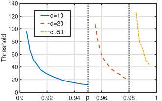
Figure 4: Thresholds of the optimal scheduling policy for i.i.d. mmWave channel state, where the packet transmission time of the sub-6GHz channel is $d=10,20,50$.

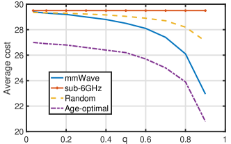
Figure 5: Time-average expected age vs. the parameter $q$ of the mmWave channel, where $d=20$ and $p=0.966$.

Proof.

By (LABEL:def1) and $1-q=p$, we have: (i) $F(p,q,d)=H(p,q,d)$, and (ii) $F(p,q,d)>0$ is equivalent to $G(p,q,d)>0$. From the two above results and the definition of $\textbf{B}_{1},\ldots,\textbf{B}_{4}$ in (5), we directly get (55) and (56). Moreover, the definitions of (55) and (56) imply that $(p,q,d)\in\textbf{B}_{1}$ or $(p,q,d)\in\textbf{B}_{3}$. ∎

From Theorem 2, if $(p,q,d)\in\textbf{B}_{1}$, then the optimal policy is always choosing Channel $1$. From Theorem 4, if $(p,q,d)\in\textbf{B}_{3}$, then the optimal policy chooses one of the five cases that are depicted in (45). However, we can reduce the five cases to two cases: If Channel $1$ is i.i.d., then the state information of Channel $1$ is not useful. Thus, $\lambda_{0}^{*}=\lambda_{1}^{*}$. Note that from Definition 2, we have $s_{2}(\beta)\leq d$ and $s_{i}(\beta)\geq d+1$ for $i\in\{1,3,4\}$. Thus, only the first case and the last case in (45) can possibly appear for i.i.d. channel.

So in i.i.d. case, Theorem 2 and Theorem 4 reduce to the following:

Corollary 1.

Suppose that $p+q=1$, i.e., Channel $1$ is i.i.d., then

(a) If $1-p\geq 1/d$, then the optimal policy is always choosing Channel $1$. In this case, the optimal objective value of (2) is $\bar{\Delta}_{\text{opt}}=1/(1-p)$.

(b) If $1-p<1/d$, then the optimal policy is non-decreasing in age and the optimal thresholds $\lambda^{*}_{0}=\lambda^{*}_{1}$. The threshold $\lambda^{*}_{0}$ may take multiple values, given by

$$\left\{\begin{array}[]{lll}\lambda^{*}_{0}=s_{1}(\beta_{1})&\text{if }\leavevmode\nobreak\ \bar{\Delta}_{\text{opt}}=\beta_{1},\\ \lambda^{*}_{0}\in\{1,2,\ldots,d\}&\text{if }\leavevmode\nobreak\ \bar{\Delta}_{\text{opt}}=(3/2)d-1/2,\par\end{array}\right.$$ (57)

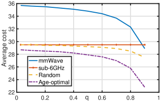
Figure 6: Time-average expected age vs. the parameter $q$ of the mmWave channel, where $d=20$ and $p=0.972$.

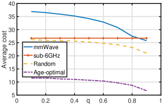
Figure 7: Time-average expected age penalty vs. the parameter $q$ of the mmWave channel, where $p=0.9$, $d=20$, and the age penalty function is $f(\Delta)=(\frac{1}{p-0.003})^{\Delta}$.

$\bar{\Delta}_{\text{opt}}$ is the optimal objective value of (2), determined by

$$\bar{\Delta}_{\text{opt}}=\min\Big{\{}\beta_{1},\frac{3}{2}d-\frac{1}{2}\Big{\}}.$$ (58)

Corollary 58(a) suggests that if the transmission rate of Channel $1$ is larger than the rate of Channel $2$ (which is $1/d$), then the age-optimal policy always chooses Channel $1$. Corollary 58(b) implies that if the transmission rate of Channel $1$ is smaller than the rate of Channel $2$, then the age-optimal policy is non-decreasing threshold-type on age.

5 Numerical Results

We first provide the optimal threshold $\lambda^{*}_{0}$ with the change of $p$ for $d=10,20,50$, respectively, where $\lambda^{*}_{0}$ is the optimal threshold in i.i.d. channel described in Corollary 58. From Fig. 4, the optimal threshold diverges to boundary $p^{*}=0.9,0.95,0.98$ respectively. As $p$ enlarges, the mmWave channel has worse connectivity, thus the thresholds goes down and converges to always choosing the sub-6GHz channel.

Then we compare our optimal scheduling policy (called Age-optimal) with three other policies, including (i) always choosing the mmWave channel (called mmWave), (ii) always choosing the sub-6GHz channel (called sub-6GHz), and (iii) randomly choosing the mmWave and sub-6GHz channels with equal probability (called Random). We provide the performance of these policies for different $q$ in Fig. 5 and Fig. 6. Our optimal policy outperforms other policies. If the two channels have a similar age performance, the benefit of the optimal policy enlarges as the mmWave channel becomes positively correlated ($q$ is larger). If the two channels have a large age performance disparity, the optimal policy is close to always choosing a single channel, and thus the benefit is obviously low. Although our theoretical results consider linear age, we also provide numerical results when the cost function is nonlinear on age by using value iteration [38]. For exponential age in Fig. 7, the gain is significantly large for all $q$: other policies have more than $2$ times of average cost than the optimal policy. The numerical simulation indicates the importance of exploring optimal policy for nonlinear age cost function, which is our future research direction.

6 conclusion

In this paper, we have studied age-optimal transmission scheduling for hybrid mmWave/sub-6GHz channels. For all possibly values of the channel parameters and the ON-OFF state of the mmWave channel, the optimal scheduling policy have been proven to be of a threshold-type on the age. Low complexity algorithms have been developed for finding the optimal scheduling policy. Finally, our numerical results show that the optimal policy can reduce age compared with other policies.

7 Appendices: Proofs of Main Results

In this section, we prove our main results: Theorem 1 (Section 7.2) and Theorem 2—5 (Section 7.3). In Section 7.1, we describe a discounted problem that helps to solve average problem (2). In Section 7.2, we introduce Proposition 1 which plays an important role in proving Theorem 1. Section 7.3 provides the proofs of Theorem 2—5.

7.1 Preliminaries

To solve Problem (2), we introduce a discounted problem below. The objective is to solve the discounted sum of expected cost given an initial state s:

$$J^{\alpha}(\textbf{s})=\inf_{\pi\in\Pi^{\prime}}\lim_{T\rightarrow\infty}\sum_{t=0}^{T}\mathbb{E}[\alpha^{t}\Delta^{\pi}(t)|\textbf{s}(0)=\textbf{s}],$$ (59)

where $\alpha\in(0,1)$ is the discount factor. We call $J^{\alpha}(\textbf{s})$ the value function given the initial state s. Recall that we use s$=(\delta,l_{1},l_{2})$ to denote the system state, where $\delta$ is the age value and $l_{1},l_{2}$ are the state of Channel $1$ and Channel $2$. From Lemma 1, we only need to consider $\pi\in\Pi^{\prime}$ instead of $\pi\in\Pi$.

The value function $J^{\alpha}(\textbf{s})$ satisfies a following property:

Lemma 4.

For any given $\alpha$ and s, $J^{\alpha}(\textbf{s})<\infty$.

Proof.

See Appendix C. ∎

A policy $\pi$ is deterministic stationary if $\pi(t)=Z(\textbf{s}(t))$ at any time $t$, where $Z:\textbf{S}\rightarrow\Pi^{\prime}$ is a deterministic function. According to [42], and Lemma 4, there is a direct result for Problem (59):

Lemma 5.

(a) The value function $J^{\alpha}(\textbf{s})$ satisfies the Bellman equation

$$\begin{split}Q^{\alpha}(\textbf{s},u)&\triangleq\delta+\alpha\sum_{\textbf{s}^{\prime}\in\textbf{S}}P_{\textbf{s}\textbf{s}^{\prime}}(u)J^{\alpha}(\textbf{s}^{\prime}),\\ J^{\alpha}(\textbf{s})&=\min_{u\in\Pi^{\prime}}Q^{\alpha}(\textbf{s},u).\end{split}$$ (60)

(b) There exists a deterministic stationary policy ${\mu}^{\alpha,*}$ that satisfies Bellman equation (60). The policy ${\mu}^{\alpha,*}$ solves Problem (59) for all initial state s.

(c) Assume that $J^{\alpha}_{0}(\textbf{s})=0$ for all s. For $n\geq 1$, $J^{\alpha}_{n}$ is defined as

$$\begin{split}Q^{\alpha}_{n}(\textbf{s},u)&\triangleq\delta+\alpha\sum_{\textbf{s}^{\prime}\in\textbf{S}}P_{\textbf{s}\textbf{s}^{\prime}}(u)J^{\alpha}_{n-1}(\textbf{s}^{\prime}),\\ J^{\alpha}_{n}(\textbf{s})&=\min_{u\in\Pi^{\prime}}Q^{\alpha}_{n}(\textbf{s},u),\end{split}$$ (61)

then $\lim_{n\rightarrow\infty}J^{\alpha}_{n}(\textbf{s})=J^{\alpha}(\textbf{s})$ for every s.

Also, since the cost function is linearly increasing in age, utilizing Lemma 5(c), we also have

Lemma 6.

For all given $l_{1}$ and $l_{2}$, $J^{\alpha}(\delta,l_{1},l_{2})$ is increasing in $\delta$.

Proof.

See Appendix D. ∎

Since Problem (59) satisfies the properties in Lemma 5, utilizing Lemma 5 and Lemma 6, the following Lemma gives the connection between Problem (2) and Problem (59).

Lemma 7.

(a) There exists a stationary deterministic policy that is optimal for Problem (2).

(b) There exists a value $J^{*}$ for all initial state s such that

$$\lim_{\alpha\rightarrow 1^{-}}(1-\alpha)J^{\alpha}(\textbf{s})=J^{*}.$$

Moreover, $J^{*}$ is the optimal average cost for Problem (2).

(c) For any sequence $(\alpha_{n})_{n}$ of discount factors that converges to $1$, there exists a subsequence $(\beta_{n})_{n}$ such that $\lim_{n\rightarrow\infty}{\mu}^{\beta_{n},*}={\mu^{*}}$. Also, ${\mu^{*}}$ is the optimal policy for Problem 2.

Proof.

See Appendix E. ∎

Lemma 7 provides the fact that: We can solve Problem (59) to achieve Problem (2). The reason is that the optimal policy of Problem (59) converges to the optimal policy of Problem (2) in a limiting scenario (as $\alpha\rightarrow 1$).

7.2 Proof of Theorem 1

We begin with providing an optimal structural result of discounted policy $\mu^{\alpha,*}$. Then, we achieve the average optimal policy ${\mu^{*}}$ by letting $\alpha\rightarrow 1$.

Definition 3.

For any discount factor $\alpha\in(0,1)$, the channel parameters $p,q\in(0,1)$ and $d\in\{2,3,...\}$, we define

$$\begin{split}\textbf{B}_{1}(\alpha)&=\{(p,q,d):F(p,q,d,\alpha)\leq 0,H(p,q,d,\alpha)\leq 0\},\\ \textbf{B}_{2}(\alpha)&=\{(p,q,d):F(p,q,d,\alpha)>0,G(p,q,d,\alpha)\leq 0\},\\ \textbf{B}_{3}(\alpha)&=\{(p,q,d):F(p,q,d,\alpha)>0,G(p,q,d,\alpha)>0\},\\ \textbf{B}_{4}(\alpha)&=\{(p,q,d):F(p,q,d,\alpha)\leq 0,H(p,q,d,\alpha)>0\},\end{split}$$ (62)

where functions $F(\cdot),G(\cdot),H(\cdot):\Theta\times(0,1)\rightarrow\mathbb{R}$ are defined as:

$$\begin{split}F(p,q,d,\alpha)&=\sum_{i=0}^{\infty}(\alpha p)^{i}-\sum_{i=0}^{d-1}\alpha^{i},\\ G(p,q,d,\alpha)&=1+\alpha(1-q)\sum_{i=0}^{d-1}\alpha^{i}-\sum_{i=0}^{d-1}\alpha^{i},\\ H(p,q,d,\alpha)&=1+\alpha(1-q)\sum_{i=0}^{\infty}(\alpha p)^{i}-\sum_{i=0}^{d-1}\alpha^{i}.\end{split}$$ (63)

Observe that all four regions $\textbf{B}_{i}(\alpha)$ converge to $\textbf{B}_{i}$ as the discount factor $\alpha\rightarrow 1$, where the regions $\textbf{B}_{i}$ are described in Definition LABEL:def1.

The optimal structural result of Problem (59) with a discount factor $\alpha$ is provided in the following proposition:

Proposition 1.

There exists a threshold type policy $\mu^{\alpha,*}(\delta,l_{1},0)$ on age $\delta$ that is the solution to Problem (59) such that:

(a) If $l_{1}=0$ and $(p,q,d)\in\textbf{B}_{1}(\alpha)\cup\textbf{B}_{4}(\alpha)$, then $\mu^{\alpha,*}(\delta,l_{1},0)$ is non-increasing in the age $\delta$.

(b) If $l_{1}=0$ and $(p,q,d)\in\textbf{B}_{2}(\alpha)\cup\textbf{B}_{3}(\alpha)$, then $\mu^{\alpha,*}(\delta,l_{1},0)$ is non-decreasing in the age $\delta$.

(c) If $l_{1}=1$ and $(p,q,d)\in\textbf{B}_{1}(\alpha)\cup\textbf{B}_{2}(\alpha)$, then $\mu^{\alpha,*}(\delta,l_{1},0)$ is non-increasing in the age $\delta$.

(d) If $l_{1}=1$ and $(p,q,d)\in\textbf{B}_{3}(\alpha)\cup\textbf{B}_{4}(\alpha)$, then $\mu^{\alpha,*}(\delta,l_{1},0)$ is non-decreasing in the age $\delta$.

Note that Theorem 1 can be immediately shown from Proposition 1, Lemma 7 and the convergence of the regions $\textbf{B}_{i}(\alpha)$ to $\textbf{B}_{i}$ (for $i=1,2,3,4$) as $\alpha\rightarrow 1$. The rest of Section 7.2 provides the proof for Proposition 1.

Since Channel $1$ and Channel $2$ have different delays, we are not able to show that the optimal policy is threshold type by directly observing the Bellman equation like [23]. Thus, we will use the concept of super-modularity [36, Theorem 2.8.2]. The domain of age set and decision set in the Q-function is $\{1,2,...\}\times\{1,2\}$, which is a lattice. Given a positive $s$, the subset $\{s,s+1,...\}\times\{1,2\}$ is a sublattice of $\{1,2,...\}\times\{1,2\}$. Thus, if the following holds for all $\delta>s$:

$$\begin{split}&Q^{\alpha}(\delta,l_{1},0,1)-Q^{\alpha}(\delta-1,l_{1},0,1)\\ \leq&Q^{\alpha}(\delta,l_{1},0,2)-Q^{\alpha}(\delta-1,l_{1},0,2),\end{split}$$ (64)

then the Q-function $Q^{\alpha}(\delta,l_{1},0,u)$ is super-modular in $(\delta,u)$ for $\delta>s$, which means the optimal decision

$$\mu^{\alpha,*}(\delta,l_{1},0)=\mathrm{argmin}_{u\in\{1,2\}}Q^{\alpha}(\delta,l_{1},0,u)$$ (65)

is non-increasing in $\delta$ for $\delta\geq s$. If the inequality of (64) is inversed, then we call $Q^{\alpha}(\delta,l_{1},0)$ is sub-modular in $(\delta,u)$ for $\delta>s$, and $\mu^{\alpha,*}(\delta,l_{1},0)$ is non-decreasing in $\delta$ for $\delta\geq s$.

For ease of notations, we give Definition 66:

Definition 4.

Given $l_{1}\in\{0,1\}$, $u\in\{1,2\}$,

$$L^{\alpha}(\delta,l_{1},u)\triangleq Q^{\alpha}(\delta,l_{1},0,u)-Q^{\alpha}(\delta-1,l_{1},0,u).$$ (66)

Note that $L^{\alpha}(\delta,l_{1},1)$ is the left hand side of (64), and $L^{\alpha}(\delta,l_{1},2)$ is the right hand side of (64).

Our high-level idea to show Proposition 1 is as follows: First, we show that $L^{\alpha}(\delta,l_{1},2)$ is a constant (see Lemma 8 below), then we compare $L^{\alpha}(\delta,l_{1},1)$ with the constant to check super-modularity (see the proofs of Lemma 9 and Lemma 10 below).

Suppose that $m\triangleq\sum_{i=0}^{d-1}\alpha^{i}$, and we have:

Lemma 8.

For all $\delta\geq 2$ and $l_{1}\in\{0,1\}$, $L^{\alpha}(\delta,l_{1},2)=m$.

Proof.

See Appendix F. ∎

Also, we have

Lemma 9.

(a) If $l_{1}=0$ and $(p,q,d)\in\textbf{B}_{1}(\alpha)\cup\textbf{B}_{4}(\alpha)$, then $Q^{\alpha}(\delta,l_{1},0,u)$ is super-modular in $(\delta,u)$ for $\delta\geq 2$.

(b) If $l_{1}=0$ and $(p,q,d)\in\textbf{B}_{2}(\alpha)\cup\textbf{B}_{3}(\alpha)$, then $Q^{\alpha}(\delta,l_{1},0,u)$ is sub-modular in $(\delta,u)$ for $\delta\geq 2$.

Proof.

See Appendix H. ∎

Lemma 9(a) implies that $\mu^{\alpha,*}(\delta,0,0)$ is non-increasing in $\delta$ if $(p,q,d)\in\textbf{B}_{1}(\alpha)\cup\textbf{B}_{4}(\alpha)$. Lemma 9(b) implies that $\mu^{\alpha,*}(\delta,0,0)$ is non-decreasing in $\delta$ if $(p,q,d)\in\textbf{B}_{2}(\alpha)\cup\textbf{B}_{3}(\alpha)$. Thus, Proposition 1(a),(b) hold.

Lemma 9 gives the result when the previous state of Channel $1$ is $0$. We then need to solve when the previous state of Channel $1$ is $1$. Different from $Q^{\alpha}(\delta,0,0,u)$, the Q-function $Q^{\alpha}(\delta,1,0,u)$ does not satisfy super-modular (or sub-modular) in ($\delta,u$) for all the age value $\delta$. Thus, we give a weakened condition: we can find out a value $s$, such that the Q-function $Q^{\alpha}(\delta,1,0,u)$ is super-modular (or sub-modular) for a partial age set $s,s+1,...$ and $\mu^{\alpha,*}(\delta,1,0)$ is a constant on the set $1,2,...,s$. Then, $\mu^{\alpha,*}(\delta,1,0)$ is still non-increasing (or non-decreasing). Note that super-/sub-modularity is the sufficient but not necessary condition to the monotonicity of $\mu^{\alpha,*}(\delta,l_{1},0)$ in $\delta$.

Thus, to solve Proposition 1(c),(d), we provide the following lemma:

Lemma 10.

(a) If $l_{1}=1$ and $(p,q,d)\in\textbf{B}_{1}(\alpha)\cup\textbf{B}_{2}(\alpha)$, then there exists a positive integer $s$, such that $Q^{\alpha}(\delta,l_{1},0,u)$ is super-modular in $(\delta,u)$ for $\delta>s$, and $\mu^{\alpha,*}(\delta,l_{1},0)$ is always $1$ or always $2$ for all $\delta\leq s$.

(b) If $l_{1}=1$ and $(p,q,d)\in\textbf{B}_{3}(\alpha)\cup\textbf{B}_{4}(\alpha)$, then there exists a positive integer $s$, such that $Q^{\alpha}(\delta,l_{1},0,u)$ is sub-modular in $(\delta,u)$ for $\delta>s$, and $\mu^{\alpha,*}(\delta,l_{1},0)$ is always $1$ or always $2$ for all $\delta\leq s$.

Proof.

See Appendix J. ∎

Lemma 10(a) implies that $\mu^{\alpha,*}(\delta,1,0)$ is non-increasing for $\delta\geq s$ and is constant for for $\delta\leq s$. Thus, $\mu^{\alpha,*}(\delta,1,0)$ is non-increasing in $\delta$. Similarly, Lemma 10(b) implies that $\mu^{\alpha,*}(\delta,1,0)$ is non-decreasing for $\delta>0$. Thus, we have shown Proposition 1(c),(d). Showing the threshold structure of $\mu^{\alpha,*}(\delta,l_{1},0)$ even if super-modularity does not hold is one of the key technical contributions in this paper.

Overall, Lemma 8 and Lemma 9 shows Proposition 1(a),(b). Lemma 8 and Lemma 10 shows Proposition 1(c),(d). Thus we have completed the proof of Proposition 1.

To summarize Section 7.2, Proposition 1, Lemma 7 and the convergence of $\textbf{B}_{1}(\alpha),\ldots,\textbf{B}_{4}(\alpha)$ to $\textbf{B}_{1},\ldots,\textbf{B}_{4}$ show Theorem 1.

7.3 Proofs of Theorem 2—Theorem 5

In this section, we prove Theorem 2$\sim$Theorem 5 with $(p,q,d)\in\textbf{B}_{1}$—$(p,q,d)\in\textbf{B}_{4}$, respectively for efficiently deriving an optimal threshold-type solution.

7.3.1 Proof of Theorem 2

For $(p,q,d)\in\textbf{B}_{1}$, we firstly prove that $\mu^{*}(\delta,0,0)=1$ and then show that $\mu^{*}(\delta,1,0)=1$.

Lemma 11.

If $(p,q,d)\in\textbf{B}_{1}\cup\textbf{B}_{4}$, then the optimal decisions at states $(\delta,0,0)$ for all $\delta$ are $1$.

Proof.

See Appendix M. ∎

In addition, when $l_{1}=1$, we have the following:

Lemma 12.

If $(p,q,d)\in\textbf{B}_{1}$, then the optimal decisions at states $(\delta,1,0)$ for all $\delta$ are $1$.

Proof.

See Appendix O. ∎

Since $\mu^{*}(\delta,1,0)$ is non-increasing in the region $\textbf{B}_{1}$ by Theorem 1, Lemma 12 implies that $\mu^{*}(\delta,1,0)=1$ for all $\delta$. Besides, Lemma 11 implies that $\mu^{*}(\delta,0,0)=1$ for all $\delta$. Thus, Theorem 2 follows directly from Lemma 11 and Lemma 12. The optimal policy for $(p,q,d)\in\textbf{B}_{1}$ is always choosing Channel $1$.

7.3.2 Proof of Theorem 3

In (9), we have stated that the MDP problem (2) is reduced to deriving the steady-state distributions of the DTMCs. Note that Channel $1$ is Markovian $(l_{1}=0$ or $1)$. When $l_{1}=1$, we observe that only the states $(1,1,0)$ and $(d,1,0)$ can be reached with positive probability for any policy in $\Pi^{\prime}$. As a result, (9) can be reduced to a number of the steady-state distributions of the DTMCs with different actions at $(1,1,0)$ and $(d,1,0)$. In addition, we observe that the state transition matrices of the DTMCs in (9) are significantly different depending on the action at $(d,0,0)$. Thus, we conclude that there are at most $2^{3}$ different steady-state distributions of DTMCs based on the actions at three system states: $(1,1,0),(d,1,0)$ with $l_{1}=1$ and $(d,0,0)$ with $l_{1}=0$. Despite that there are totally $2^{3}$ cases to enumerate, we manage to reduce to only $4$ cases as in (35) (for $(p,q,d)\in\textbf{B}_{2}$). The reason is that the remaining cases are impossible to occur due to the two following restrictions: (1) the monotonicity is known by Theorem 1, and (2) the following lemma:

Lemma 13.

If Channel $1$ is positive-correlated, i.e., $p+q\geq 1$, and $\mu^{*}(\delta,0,0)=1$, then $\mu^{*}(\delta,1,0)=1$. Conversely, if Channel $1$ is negative-correlated, i.e. $p+q\leq 1$, and $\mu^{*}(\delta,0,0)=2$, then $\mu^{*}(\delta,1,0)=2$.

Proof.

See Appendix K. ∎

Since our optimal policy is of threshold-type, the action at $(d,0,0)$ is equivalent to whether the threshold of $\mu^{*}(\delta,0,0)$ is larger or smaller than $d$. Thus, we use $s$ to denote the possible threshold of $\mu^{*}(\delta,0,0)$.

For $(p,q,d)\in\textbf{B}_{2}$, $\mu^{*}(\delta,1,0)$ is non-increasing, and $\mu^{*}(\delta,0,0)$ is non-decreasing. Note that $(p,q,d)\in\textbf{B}_{2}$ implies $p+q\geq 1$. According to Lemma 13, if $\mu^{*}(1,1,0)=2$, then $\mu^{*}(1,0,0)=2$, hence $\mu^{*}(\delta,0,0)=2$ for all $\delta$. Thus, there are two possible types of DTMCs regarding $\mu^{*}(d,1,0)=1$ or $\mu^{*}(d,1,0)=2$. If $\mu^{*}(1,1,0)=1$, then $\mu^{*}(\delta,1,0)=1$ for all $\delta$, there are thus two possible types of DTMCs regarding the threshold $s>d$ or $s\leq d$. Thus, for $(p,q,d)\in\textbf{B}_{2}$, there are four possible ways to represent the DTMC diagram of the threshold policy based on the value of the threshold $s$ and the actions at states $(d,l_{1},0)$ and $(1,1,0)$ (see Appendix P for the corresponding DTMCs and derivations):

• The threshold $s>d$ and $\mu^{*}(1,1,0)=\mu^{*}(d,1,0)=1$ ($\lambda^{*}_{1}=1$). Note that we have mentioned $\bar{\Delta}_{2}(\lambda_{0},\lambda_{1})$ as the average age of the DTMC with thresholds $(\lambda_{0},\lambda_{1})$ when $(p,q,d)\in\textbf{B}_{2}$. Then, the average age is derived as $\bar{\Delta}_{2}(s,1)=f_{1}(s)/g_{1}(s)$, which is shown in Appendix P.1. The functions $f_{1}(s),g_{1}(s)$ are described in Table II. As is shown later, $\beta_{1}$ described in Definition 2 is the minimum of $f_{1}(s)/g_{1}(s)$.

• The threshold $s\leq d$ and $\mu^{*}(1,1,0)=\mu^{*}(d,1,0)=1$ ($\lambda^{*}_{1}=1$). Then the average age is $\bar{\Delta}_{2}(s,1)=f_{2}(s)/g_{2}(s)$, which is shown in Appendix P.2. The functions $f_{2}(s),g_{2}(s)$ are described in Table II. As is shown later, $\beta_{2}$ described in Definition 2 is the minimum of $f_{2}(s)/g_{2}(s)$.

• The threshold $s=1$, $\mu^{*}(1,1,0)=2$ and $\mu^{*}(d,1,0)=1$ ($\lambda^{*}_{1}\in\{2,3,...,d\}$). The average age is the constant $f_{0}/g_{0}$, which is shown in Appendix P.3. Note that $f_{0}/g_{0}$ is described in Theorem 3.

• The threshold $s=1$ and $\mu^{*}(1,1,0)=\mu^{*}(d,1,0)=2$ ($\lambda^{*}_{1}\in\{d+1,d+2,...\}$). This policy means that we always choose Channel $2$. So the average age is $(3/2)d-1/2$.

The listed statements illustrated above directly provides the following property:

Proposition 2.

If $(p,q,d)\in\textbf{B}_{2}$, then the optimal scheduling policy is

$$\mu^{*}(\delta,0,0)=\left\{\begin{array}[]{lll}1&\text{if }\leavevmode\nobreak\ \delta<\lambda_{0}^{*};\\ 2&\text{if }\leavevmode\nobreak\ \delta\geq\lambda_{0}^{*},\end{array}\right.$$ (69)

$$\mu^{*}(\delta,1,0)=\left\{\begin{array}[]{lll}2&\text{if }\leavevmode\nobreak\ \delta<\lambda_{1}^{*};\\ 1&\text{if }\leavevmode\nobreak\ \delta\geq\lambda_{1}^{*},\end{array}\right.$$ (72)

where $\lambda_{0}^{*}$ and $\lambda_{1}^{*}$ are given by

$$\!\!\!\!\!\left\{\begin{array}[]{lll}\lambda_{0}^{*}=\underset{s\in\{d+1,\ldots\}}{\operatorname*{argmin}}f_{1}(s)/g_{1}(s),\lambda_{1}^{*}=1\ \ \ \text{if }\leavevmode\nobreak\ \bar{\Delta}_{\text{opt}}=\beta_{1}^{\prime},\\ \lambda_{0}^{*}=\underset{s\in\{1,\ldots,d\}}{\operatorname*{argmin}}f_{2}(s)/g_{2}(s),\ \lambda_{1}^{*}=1\ \ \ \text{if }\leavevmode\nobreak\ \bar{\Delta}_{\text{opt}}=\beta_{2}^{\prime},\\ \lambda_{0}^{*}=1,\ \ \ \lambda_{1}^{*}\in\{2,3,\ldots,d\}\ \ \ \ \text{if }\leavevmode\nobreak\ \bar{\Delta}_{\text{opt}}=f_{0}/g_{0},\\ \lambda_{0}^{*}=1,\ \ \ \lambda_{1}^{*}\in\{d+1,\ldots\}\ \ \ \ \ \text{if }\leavevmode\nobreak\ \bar{\Delta}_{\text{opt}}=(3/2)d-1/2,\end{array}\right.\!\!\!\!\!$$ (73)

$\bar{\Delta}_{\text{opt}}$ is the optimal objective value of (2), determined by

$$\bar{\Delta}_{\text{opt}}=\min\Big{\{}\beta_{1}^{\prime},\beta_{2}^{\prime},\frac{f_{0}}{g_{0}},\frac{3}{2}d-\frac{1}{2}\Big{\}},$$ (74)

$\beta_{1}^{\prime}$, $\beta_{2}^{\prime}$ are given in (36), (37), respectively.

By using Dinkelbach’s method [43], we can change the minimization problem (36), (37) into a two-layer problem. The inner-layer problem is shown to be unimodal and we derive an exact solution. Thus, we only need a bisection algorithm for the outer-layer, i.e., solving the roots of the equations $h_{1}(\beta)=0,h_{2}(\beta)=0$ in (25). To show this, we introduce the following lemma:

Lemma 14.

Suppose that $i\in\{1,2,3,4\}$. Define

$$h^{\prime}_{i}(c) =\min_{s\in\{d+1,...\}}f_{i}(s)-cg_{i}(s),\ i\in\{1,3,4\},$$ (75)

$$h^{\prime}_{2}(c) =\min_{s\in\{2,...d\}}f_{2}(s)-cg_{2}(s),$$ (76)

then for all $i=1,2,3,4$, $h^{\prime}_{i}(c)\lesseqqgtr 0$ if and only if $c\gtreqqless\beta^{\prime}_{i}$.

Proof.

See Appendix Q. ∎

The solution to $h^{\prime}_{i}(c)$ in Lemma 14 is shown in the following lemma:

Lemma 15.

Suppose that $i\in\{1,2,3,4\}$. If $(p,q,d)\in\textbf{B}_{2}\cup\textbf{B}_{3}$, then the threshold $s_{i}(c)$ defined in (26) is the solution to (75) and (76), i.e., $h_{i}(c)=h^{\prime}_{i}(c)$.

Proof.

See Appendix R. ∎

Therefore, we can immediately conclude that for all $i\in\{1,2,3,4\}$:

$$\beta^{\prime}_{i}=\beta_{i},$$ (77)

where $\beta^{\prime}_{i}$ is defined in (36), (37) and $\beta_{i}$ is derived in Definition 2 with low complexity algorithm. In addition,

$$s_{i}(\beta_{i}) =\underset{s\in\{d+1,\ldots\}}{\operatorname*{argmin}}f_{i}(s)/g_{i}(s),i\in\{1,3,4\},$$ (78)

$$s_{2}(\beta_{2}) =\underset{s\in\{2,\ldots,d\}}{\operatorname*{argmin}}f_{2}(s)/g_{2}(s).$$ (79)

The studies in [11, 21, 10] also derive an exact solution to their inner-layer problem. However, their technique is using optimal stopping rules [21, 11] or stochastic convex optimization [10], which is different with our study. In conclusion, (77) and Proposition 2 shows Theorem 3.

7.3.3 Proof of Theorem 4

When $(p,q,d)\in\textbf{B}_{3}$ , $\mu^{*}(\delta,0,0)$ and $\mu^{*}(\delta,1,0)$ are non-decreasing. Then, the two cases are removed: $\mu^{*}(\delta,0,0)=2$, $\mu^{*}(\delta,1,0)=1$, $s\leq d$ or $s>d$. Since $(p,q,d)\in\textbf{B}_{3}$ does not imply $p+q\leq 1$ or $p+q\geq 1$, we will enumerate all of the five possible ways to represent the DTMCs of the threshold policy based on the value of the threshold $s$ and the optimal decision at states $(d,1,0)$ and $(1,1,0)$ (see Appendix P for the corresponding DTMCs):

• The threshold $s>d$ and $\mu^{*}(1,1,0)=\mu^{*}(d,1,0)=1$ ($\lambda^{*}_{1}\in\{d+1,d+2,...\}$). The average age is derived as $f_{1}(s)/g_{1}(s)$.

• The threshold $s>d$, $\mu^{*}(1,1,0)=1$ and $\mu^{*}(d,1,0)=2$ ($\lambda^{*}_{1}\in\{2,...,d\}$). Then, the average age is $f_{3}(s)/g_{3}(s)$, which is shown in Appendix P.4.

• The threshold $s>d$ and $\mu^{*}(1,1,0)=\mu^{*}(d,1,0)=2$ ($\lambda^{*}_{1}\in\{2,...,d\}$) with average age $f_{4}(s)/g_{4}(s)$, which is shown in Appendix P.5.

• The threshold $s\leq d$ and $\mu^{*}(1,1,0)=\mu^{*}(d,1,0)=1$ ($\lambda^{*}_{1}\in\{d+1,d+2,...\}$), with average age $f_{2}(s)/g_{2}(s)$.

• The threshold $s\leq d$ and $\mu^{*}(d,1,0)=2$. Then, regardless of $\mu^{*}(1,1,0)$ ($\lambda^{*}_{1}\in\{1,2,...,d\}$), the DTMC corresponds to always choosing $2$, with average age $(3/2)d-1/2$.

Then, we directly have the following result:

Proposition 3.

If $(p,q,d)\in\textbf{B}_{3}$, then the optimal scheduling policy is

$$\mu^{*}(\delta,0,0)=\left\{\begin{array}[]{lll}1&\text{if }\leavevmode\nobreak\ \delta<\lambda_{0}^{*};\\ 2&\text{if }\leavevmode\nobreak\ \delta\geq\lambda_{0}^{*},\end{array}\right.$$ (82)

$$\mu^{*}(\delta,1,0)=\left\{\begin{array}[]{lll}1&\text{if }\leavevmode\nobreak\ \delta<\lambda_{1}^{*};\\ 2&\text{if }\leavevmode\nobreak\ \delta\geq\lambda_{1}^{*},\end{array}\right.$$ (85)

where $\lambda_{0}^{*}$ and $\lambda_{1}^{*}$ are given by

$$\!\!\!\!\left\{\begin{array}[]{lll}\lambda_{0}^{*}=\underset{s\in\{d+1,\ldots\}}{\operatorname*{argmin}}f_{1}(s)/g_{1}(s),\lambda_{1}^{*}\in\{d+1,\ldots\}\ \text{if\leavevmode\nobreak\ }\bar{\Delta}_{\text{opt}}=\beta_{1}^{\prime},\\ \lambda_{0}^{*}=\underset{s\in\{2,\ldots,d\}}{\operatorname*{argmin}}f_{2}(s)/g_{2}(s),\ \lambda_{1}^{*}\in\{d+1,\ldots\}\ \text{if\leavevmode\nobreak\ }\bar{\Delta}_{\text{opt}}=\beta_{2}^{\prime},\\ \lambda_{0}^{*}=\underset{s\in\{d+1,\ldots\}}{\operatorname*{argmin}}f_{3}(s)/g_{3}(s),\lambda_{1}^{*}\in\{2,\ldots,d\}\ \ \ \text{if\leavevmode\nobreak\ }\bar{\Delta}_{\text{opt}}=\beta_{3}^{\prime},\\ \lambda_{0}^{*}=\underset{s\in\{d+1,\ldots\}}{\operatorname*{argmin}}f_{4}(s)/g_{4}(s),\lambda_{1}^{*}\in\{2,\ldots,d\}\ \ \ \text{if\leavevmode\nobreak\ }\bar{\Delta}_{\text{opt}}=\beta_{4}^{\prime},\\ \lambda_{0}^{*}=1,\ \ \ \lambda_{1}^{*}\in\{1,2,\ldots,d\}\ \ \ \text{if\leavevmode\nobreak\ }\bar{\Delta}_{\text{opt}}=(3/2)d-1/2,\end{array}\right.\!\!\!\!$$ (86)

$\bar{\Delta}_{\text{opt}}$ is the optimal objective value of (2), determined by

$$\bar{\Delta}_{\text{opt}}=\min\Big{\{}\beta_{1}^{\prime},\beta_{2}^{\prime},\beta_{3}^{\prime},\beta_{4}^{\prime},\frac{3}{2}d-\frac{1}{2}\Big{\}}.$$ (87)

According to (77), (78) and (79), Theorem 4 is shown directly from Proposition 3.

7.3.4 Proof of Theorem 5

For $(p,q,d)\in\textbf{B}_{4}$, $\mu^{*}(\delta,1,0)$ is non-decreasing in $\delta$ from Theorem 1. Also, $\mu^{*}(\delta,0,0)=1$ by Lemma 11.

If $\mu^{*}(1,1,0)=1$, the policy becomes always choosing Channel $1$ (since $(d,1,0)$ is not reached at any time slot with probability $1$). If $\mu^{*}(1,1,0)=2$, then $\mu^{*}(\delta,1,0)=2$ for all $\delta$. Thus, the solution to the optimal threshold-type policy when $(p,q,d)\in\textbf{B}_{4}$ may contain two possible steady-state DTMCs which directly gives Theorem 5:

• The optimal decision $\mu^{*}(\delta,0,0)=1$ for all $\delta\geq 1$ and $\mu^{*}(1,1,0)=1$. Then, the optimal policy is always choosing Channel $1$. The average age of always choosing Channel $1$ is $((1-q)(2-p)+(1-p)^{2})/((2-q-p)(1-p))$ as in (12).

• The optimal decision $\mu^{*}(\delta,0,0)=1$ and $\mu^{*}(\delta,1,0)=2$ for all $\delta\geq 1$. See Appendix P for the corresponding DTMC. The average age by analyzing the steady-state distribution of this DTMC is $f^{\prime}_{0}/g^{\prime}_{0}$ which is shown in Appendix P.6.

Therefore, the listed items directly proves Theorem 5.

From our analysis in Section 7.3, we have the following conclusion for the proof of Theorem 2-5: (i) If $(p,q,d)\in\textbf{B}_{1}$, the optimal decision is always choosing Channel $1$; (ii) If $(p,q,d)\in\textbf{B}_{2}$, $\textbf{B}_{3}$ or $\textbf{B}_{4}$, there are a couple of possible cases ($4$ cases for $(p,q,d)\in\textbf{B}_{2}$, $5$ cases for $(p,q,d)\in\textbf{B}_{3}$ and $2$ cases for $(p,q,d)\in\textbf{B}_{4}$, respectively). Each case corresponds to analyzing the steady-state distribution of a single DTMC or a collection of DTMCs over the threshold $s$; in the latter case, the optimal threshold can be computed efficiently using bisection search. The optimal objective value in (2) is the minimum of the derived ages in each cases and the optimal thresholds are determined by the case that achieves the minimum.

Table II: Notations for $f_{i}(s),g_{i}(s),l_{i},o_{i}$ $(i=1,2,3,4)$ in Definition 2

Name	Expression
	$\begin{bmatrix}a^{\prime}_{d}&b^{\prime}_{d}\\ a_{d}&b_{d}\end{bmatrix}=\begin{bmatrix}q&1-q\\ 1-p&p\end{bmatrix}^{d}$
$f_{0}$	$q\sum_{i=1}^{d}i+(1-q)\sum_{i=d+1}^{2d}i+(\frac{b^{\prime}_{d}q+b_{d}}{1-b_{d}}+1)\sum_{i=d+1}^{2d}i$
$g_{0}$	$\frac{b^{\prime}_{d}q+b_{d}}{1-b_{d}}d+d+1$
$f^{\prime}_{0}$	$\sum_{i=1}^{d}i+a^{\prime}_{d}/b^{\prime}_{d}\times\sum_{i=d}^{2d-1}i+\sum_{i=d}^{\infty}ip^{i-d}$
$g^{\prime}_{0}$	$d/b^{\prime}_{d}+1/(1-p)$
$c_{1}(s)$	$1-b_{d}p^{s-d}-(1-q)a_{d}p^{s-d-1}$
$f_{1}(s)$	$c_{1}(s)(p/(1-q)+\sum_{i=2}^{d}ip^{i-1})+dp^{d}$
	$+\sum_{i=d+1}^{s-1}ip^{i-1}+\sum_{i=s}^{s+d-1}ip^{s-1}$
$g_{1}(s)$	$c_{1}(s)(p/(1-q)+\sum_{i=2}^{d}p^{i-1})+p^{d}$
	$+\sum_{i=d+1}^{s-1}p^{i-1}+\sum_{i=s}^{s+d-1}p^{s-1}$
$c_{2}$	$b_{d}/(a_{d}q)$
$f_{2}(s)$	$(p/(1-q)+\sum_{i=2}^{s}ip^{i-1})+\sum_{i=s+1}^{s+d-1}ip^{s-1}$
	$+c_{2}\sum_{i=d-1}^{2d-1}ip^{s-1}+(\sum_{i=d+1}^{2d}(1-q)i+d)p^{s-1}/q$
$g_{2}(s)$	$(p/(1-q)+\sum_{i=2}^{s}p^{i-1})+(d-1)p^{s-1}+c_{2}dp^{s-1}$
	$+(d(1-q)+1)p^{s-1}/q$
$f_{3}(s)$	$(1-p^{s-d})(p/(1-q)+\sum_{i=2}^{d-1}ip^{i-1})$
	$+\sum_{i=d}^{s}ip^{i-1}+\frac{a_{d}}{b^{\prime}_{d}}p^{s-1}\sum_{i=d}^{2d-1}i+\sum_{i=s+1}^{s+d-1}ip^{s-1}$
$g_{3}(s)$	$(1-p^{s-d})(p/(1-q)+\sum_{i=2}^{d-1}p^{i-1})$
	$+\sum_{i=d}^{s}p^{i-1}+\frac{a_{d}}{b^{\prime}_{d}}p^{s-1}d+(d-1)p^{s-1}$
$c_{4}(s)$	$(a^{\prime}_{d}+(a_{d}-a^{\prime}_{d})p^{s-d})/(b^{\prime}_{d})$
$f_{4}(s)$	$(1-p^{s-d})\sum_{i=1}^{d}i+c_{4}(s)\sum_{i=d}^{2d-1}i$
	$+\sum_{i=s+1}^{s+d-1}ip^{s-d}+\sum_{i=d}^{s}ip^{i-d}$
$g_{4}(s)$	$(1-p^{s-d})d+c_{4}(s)d+(d-1)p^{s-d}$
	$+\sum_{i=d}^{s}p^{i-d}$
$l^{\prime}_{1}$	$-p^{-d+1}(b_{d}+(1-q)a_{d})(1-p)(p/(1-q)+\sum_{i=2}^{d}ip^{i-1})$
	$+d(p-(1-p)(d-1)/2)$
$o_{1}$	$-p^{-d+1}(b_{d}+(1-q)a_{d})(1-p)(p/(1-q)+\sum_{i=2}^{d}p^{i-1})$
	$+1-(1-p)d$
$l^{\prime}_{2}$	$-c_{2}(1-p)\sum_{i=d-1}^{2d-1}-(\sum_{i=d+1}^{2d}(1-q)i+d+1)(1-p)/q$
	$+d(p-(1-p)(d-1)/2)$
$o_{2}$	$p-(1-p)(1+d(1-q))/q$
	$-(1-p)d(1+c_{2})$
$l^{\prime}_{3}$	$(p/(1-q)+\sum_{i=2}^{d-1}ip^{i-d}(1-p))-\sum_{i=d}^{2d-1}i(1-p)a_{d}/b^{\prime}_{d}$
	$+(d-1)(p-d(1-p)/2)$
$o_{3}$	$(p/(1-q)+\sum_{i=2}^{d-1}p^{i-d}(1-p))$
	$+1-(1-p)(d-1+da_{d}/b^{\prime}_{d})$
$p^{d-1}l^{\prime}_{4}$	$-(1-p)\sum_{i=1}^{d-1}i-\sum_{i=d}^{2d-1}(1-p)/(1-a_{d})$
	$+(d-1)(p-d(1-p)/2)$
$p^{d-1}o_{4}$	$-(1-p)d-(1-p)d/(1-a_{d})-(d-1)(1-p)+1$

Appendix A Proof of Lemma 1

Suppose that the age at initial time $0$ is the same for any policy. For any given policy $\pi\in\Pi$, we construct a policy $\pi^{\prime}$: whenever both channels are idle and $\pi$ chooses none, $\pi^{\prime}$ chooses Channel $1$, and at other time $\pi$ and $\pi^{\prime}$ are the same. The equivalent expression of $\pi^{\prime}$ is given as follows:

$$\pi^{\prime}(t)=\left\{\begin{array}[]{lll}1&\text{if }l_{2}(t)=0\text{ and }\pi(t)=\emph{none};\\ \pi(t)&\text{else.}\end{array}\right.$$ (88)

The policy $\pi$ and $\pi^{\prime}$ are coupled given a sample path of Channel $1$: $\mathcal{I}=\{l_{1}(0),l_{1}(1),\ldots\}$. For any $\mathcal{I}$, we want to show that the age of policy $\pi^{\prime}$ is smaller or equal to that of $\pi$.

For simplicity, we use $\Delta_{\pi}(t)$ and $l_{2}(t)$ to be the age and the state of Channel $2$, respectively, with a policy $\pi$ and $\mathcal{I}$. Compared with $\pi$, $\pi^{\prime}$ only replaces none by $1$. Thus, the state of Channel $2$ of $\pi^{\prime}$ is still $l_{2}(t)$.

Then, we will show that for all time $t$ and any $\mathcal{I}$, the age $\Delta_{\pi^{\prime}}(t)\leq\Delta_{\pi}(t)$. We prove by using induction.

If $t=0$, then according to our assumption, the hypothesis trivially holds.

Suppose that the hypothesis holds for $t=k$. We will show for $t=k+1$.We divide the proof into two different conditions: (i) If $l_{2}(k)>0$, then $\pi(k)=\pi^{\prime}(k)=\emph{none}$. Thus,

$$\begin{split}&\Delta_{\pi}(k+1)=\left\{\begin{array}[]{lll}\Delta_{\pi}(k)+1&\text{if }l_{2}(k)\geq 2;\\ d&\text{if }l_{2}(k)=1,\end{array}\right.\\ &\Delta_{\pi^{\prime}}(k+1)=\left\{\begin{array}[]{lll}\Delta_{\pi^{\prime}}(k)+1&\text{if }l_{2}(k)\geq 2;\\ d&\text{if }l_{2}(k)=1.\end{array}\right.\end{split}$$ (89)

Thus, $\Delta_{\pi^{\prime}}(k+1)\leq\Delta_{\pi}(k+1)$.

(ii) If $l_{2}(k)=0$, then $\pi(k)$ may take none, $1$, or $2$. If $\pi(k)=1$ or $2$, then $\pi^{\prime}(k)=\pi(k)$. Thus, the hypothesis directly gives $\Delta_{\pi^{\prime}}(k+1)\leq\Delta_{\pi}(k+1)$. If $\pi(k)=\emph{none}$, then $\pi^{\prime}(k)=1$. Then,

$$\begin{split}&\Delta_{\pi^{\prime}}(k+1)\leq\Delta_{\pi^{\prime}}(k)+1,\\ &\Delta_{\pi}(k+1)=\Delta_{\pi}(k)+1.\end{split}$$ (90)

Thus, $\Delta_{\pi^{\prime}}(k+1)\leq\Delta_{\pi}(k+1)$. From (i) and (ii), we complete the proof of induction.

Appendix B Proof of Lemma 2

Similar techniques were also used recently in [21].

(1) According to Lemma 15, the function $h_{i}(\beta)$ in (25) also satisfies

$$h_{i}(\beta) =\min_{s\in\{d+1,...\}}f_{i}(s)-\beta g_{i}(s),\ i\in\{1,3,4\},$$ (91)

$$h_{2}(\beta) =\min_{s\in\{1,...d\}}f_{2}(s)-\beta g_{2}(s),$$ (92)

The function $f_{i}(s)-\beta g_{i}(s)$ is linearly decreasing, which is concave and continuous. Since the minimization preserves the concavity and continuity, $h_{i}(\beta)$ is still concave. From Table II, it is easy to show that there exists a positive $d^{\prime}$ such that $f_{i}(s)>d^{\prime}$ and $g_{i}(s)>d^{\prime}$ for all $i\in\{1,2,3,4\}$. So, for all $s$ and any $\beta_{1}<\beta_{2}$, $f_{i}(s)-\beta_{1}g_{i}(s)>f_{i}(s)-\beta_{2}g_{i}(s)$. Thus, $h_{i}(\beta)$ is strictly decreasing.

(2) Since $f_{i}(s)>d^{\prime}$ and $g_{i}(s)>d^{\prime}$, so $h_{i}(0)>0$. Moreover, since $h_{i}(\beta)$ is strictly decreasing, we have $\lim_{\beta\rightarrow\infty}h_{i}(\beta)=-\infty$.

Appendix C proof of Lemma 4

Consider the policy that always idles at every time slot (i.e., $\pi(t)=\emph{none}$ for all $t$). Under this policy, the age increases linearly with time. The discounted cost under the aforementioned policy acts as an upper bound on the optimal value function $J^{\alpha}(\textbf{s})$. Thus, for any initial state $s=(\delta,l_{1},l_{2})$, $J^{\alpha}(\textbf{s})$ satisfies

$$J^{\alpha}(\textbf{s})\leq\delta+\alpha(\delta+1)+\alpha^{2}(\delta+2)...=\frac{(\delta+\frac{\alpha}{1-\alpha})}{1-\alpha}<\infty,$$ (93)

which proves the result.

Appendix D proof of Lemma 6

We show Lemma 6 by using induction in value iteration (61). We want to show that $J^{\alpha}_{n}(\textbf{s})=J^{\alpha}_{n}(\delta,l_{1},l_{2})$ is increasing in age $\delta$ for all iteration number $n$.

If $n=0$, $J^{\alpha}_{0}(\delta,l_{1},l_{2})=0$, so the hypothesis holds. Suppose the hypothesis holds for $n=k$, then we will show that it also holds for $n=k+1$. First, note that in (61), the immediate cost of any state $\textbf{s}=(\delta,l_{1},l_{2})$ is $\delta$, which is increasing in age. Second, by our hypothesis and the evolution of age in Section 3 , $\sum_{\textbf{s}^{\prime}\in\textbf{S}}P_{\textbf{s}\textbf{s}^{\prime}}(u)J^{\alpha}_{k}(\textbf{s}^{\prime})$ is increasing in age $\delta$. Thus, $Q^{\alpha}_{k+1}(\textbf{s},u)$ is increasing in age $\delta$. Thus, $J^{\alpha}_{k+1}(\textbf{s})$ is increasing in age $\delta$ and we have completed the induction.

Appendix E Proof of Lemma 7

Similar techniques were also used recently in [13].

According to [42] and Lemma 4, it is sufficient to show that Problem (2) satisfies the following two conditions:

(a) There exists a non-negative function $M({\textbf{s}})$ such that $h^{\alpha}(\textbf{s})\leq M({\textbf{s}})$ for all s and $\alpha$, where the relative function $h^{\alpha}(\textbf{s})=J^{\alpha}(\textbf{s})-J^{\alpha}(1,1,0)$.

(b) There exists a non-negative $N$ such that $-N\leq h^{\alpha}(\textbf{s})$ for all the state s and $\alpha$.

For (a), we first consider a stationary deterministic policy $f$ that always chooses Channel $1$. The states $(1,1,0)$, $(\delta,0,0)$ ($\delta\geq 2$) are referred as recurrent states. The remaining states in the state space are referred as transient states. Define $e(\textbf{s}_{1},\textbf{s}_{2})$ to be the average cost of the first passage from $\textbf{s}_{1}$ to $\textbf{s}_{2}$ under the policy $f$ where $\textbf{s}_{1}$ and $\textbf{s}_{2}$ are recurrent states. The recurrent states of $f$ form an aperiodic, recurrent and irreducible Markov chain. So, from Proposition $4$ in [42], for any recurrent state $\textbf{s}^{\prime}$, $e({\textbf{s}^{\prime},\textbf{s}_{0}})$ is finite (where $\textbf{s}_{0}=(1,1,0)$).

Now, we pick $M({\textbf{s}})$. We let $M({\textbf{s}})=e({\textbf{s}^{\prime},\textbf{s}_{0}})+d(\delta+d-1)$ for the transient state s, and let $M({\textbf{s}})=e({\textbf{s},\textbf{s}_{0}})$ for the recurrent state s. Then, replacing ”$BE_{\theta}(T)$” by $M(\textbf{s})$ in the proof of Proposition $1$ in [44], we have $h^{\alpha}(\textbf{s})\leq M({\textbf{s}})$ for all the state s. Overall, there exists $M({\textbf{s}})$ such that $h^{\alpha}(\textbf{s})\leq M({\textbf{s}})$.

We start to show (b). According to Lemma 6, the value function is increasing in age. Thus, we only need to show that there exists $N$ such that $-N\leq h^{\alpha}(1,l_{1},l_{2})$ for all $l_{1}$ and $l_{2}$. In order to prove this, we will show that there exists $E^{\prime}(1,l_{1},l_{2})$ such that $-E^{\prime}(1,l_{1},l_{2})\leq h^{\alpha}(1,l_{1},l_{2})$ for all $l_{1}$ and $l_{2}$. Thus, we take $N=\max_{l_{1}\in\{0,1\},l_{2}\in\{0,1,...,d-1\}}E^{\prime}(1,l_{1},l_{2})$, which is still finite, and condition (b) is shown.

Now, we start to find out $E^{\prime}(1,l_{1},l_{2})$.

We split the states $(1,l_{1},l_{2})$ into three different cases.

$(b1)$ If $l_{1}=1$ and $l_{2}=0$, then $h^{\alpha}(1,l_{1},l_{2})=0$. Thus, we take $E^{\prime}(1,l_{1},l_{2})=0$.

$(b2)$ If $l_{1}=0$ and $l_{2}=0$, then we take $T=1$ if the optimal decision of $(1,0,0)$ is $1$ and take $T=d+1$ if the optimal decision is $2$. Therefore, the definition of $J^{\alpha}(1,0,0)$ tells that there exists $T\in\{1,d+1\}$ and $a\in[0,1]$ such that

$$\begin{split}&J^{\alpha}(1,0,0)\\ \geq&\sum_{i=1}^{T}i\alpha^{i-1}+\alpha^{T}\left(aJ^{\alpha}(1,1,0)+(1-a)J^{\alpha}(1,0,0)\right)\\ \geq&\alpha^{T}(aJ^{\alpha}(1,1,0)+(1-a)J^{\alpha}(1,0,0))\\ =&\alpha^{T}\Big{(}aJ^{\alpha}(1,1,0)+(1-a)(h^{\alpha}(1,0,0)+J^{\alpha}(1,1,0))\Big{)}\\ =&\alpha^{T}J^{\alpha}(1,1,0)+\alpha^{T}(1-a)h^{\alpha}(1,0,0)\\ \geq&\alpha^{T}J^{\alpha}(1,1,0)+\alpha^{T}(1-a)h^{\alpha}(1,0,0).\end{split}$$ (94)

Notice that $J^{\alpha}(1,1,0)$ is smaller or equal to the $\alpha$-discounted cost of always choosing Channel $1$ with initial state $(1,1,0)$. Consider a special case of MDP consisting of states $(1,1,0),(2,0,0),(3,0,0),\ldots,$ where there is only one policy that always chooses Channel $1$. Therefore, applying Lemma A2 in appendix of [42] to this MDP, $(1-\alpha)J^{\alpha}(1,1,0)$ is upper bounded by a constant $c^{\prime}$ that is not a function of $\alpha$. Note that

$$1-\alpha^{T}=(1-\alpha)(1+\alpha+...+\alpha^{T-1})\leq(1-\alpha)T.$$ (95)

Then from (94), we get

$$\begin{split}&h^{\alpha}(1,0,0)\\ =&J^{\alpha}(1,0,0)-J^{\alpha}(1,1,0)\\ \geq&-(1-\alpha^{T})J^{\alpha}(1,1,0)+\alpha^{T}(1-a)h^{\alpha}(1,0,0)\\ \geq&-Tc^{\prime}+\alpha^{T}(1-a)h^{\alpha}(1,0,0).\\ \end{split}$$ (96)

Therefore,

$$h^{\alpha}(1,0,0)\geq-\frac{Tc^{\prime}}{1-\alpha^{T}(1-a)}\triangleq E^{\prime}(1,0,0).$$ (97)

$(b3)$ If $l_{2}>0$, similar with $(b2)$, we take $T^{\prime}=l_{2}$ and there exists $a^{\prime}\in[0,1]$ such that

$$h^{\alpha}(1,l_{1},l_{2}) \geq-T^{\prime}c^{\prime}-\alpha^{T^{\prime}}(1-a^{\prime})\frac{Tc^{\prime}}{1-\alpha^{T}(1-a)}$$ (98)

$$\triangleq E^{\prime}(1,l_{1},l_{2}).$$ (99)

Therefore, we have found out all the values of $E^{\prime}(1,l_{1},l_{2})$. Overall, by proving (a) and (b), we complete the proof of Lemma 7.

Appendix F proof of Lemma 8

Recall that we use $l_{1}$ (which is $0$ or $1$) to denote the state of Channel $1$ and that

$$L^{\alpha}(\delta,l_{1},2)=Q^{\alpha}(\delta,l_{1},0,2)-Q^{\alpha}(\delta-1,l_{1},0,2)$$ (100)

. We define the sequences $a_{k}$, $a^{\prime}_{k}$, $b_{k}$, $b^{\prime}_{k}$ with the non-negative index $k$ as

$$[a_{k},b_{k}]=[0,1]\times P^{k},\ \ \ [a^{\prime}_{k},b^{\prime}_{k}]=[1,0]\times P^{k},$$ (101)

where $P$ is the transition probability matrix of Channel $1$, given by $\begin{bmatrix}q&1-q\\ 1-p&p\end{bmatrix}$. Note that (101) implies $a_{k}+b_{k}=a^{\prime}_{k}+b^{\prime}_{k}=1$ for all the index $k$.

By using the Bellman equation (60) iteratively, $L^{\alpha}(\delta,0,2)$ and $L^{\alpha}(\delta,1,2)$ satisfy the following lemma:

Lemma 16.

The values $L^{\alpha}(\delta,0,2)$ and $L^{\alpha}(\delta,1,2)$ satisfy:

$$\begin{split}&L^{\alpha}(\delta,0,2)=\sum_{i=0}^{d-2}\alpha^{i}\\ &+\alpha^{d-1}a_{d-1}\Big{(}J^{\alpha}(\delta+d-1,1,1)-J^{\alpha}(\delta+d-2,1,1)\Big{)}\\ &+\alpha^{d-1}b_{d-1}\Big{(}J^{\alpha}(\delta+d-1,0,1)-J^{\alpha}(\delta+d-2,0,1)\Big{)},\\ &L^{\alpha}(\delta,1,2)=\sum_{i=0}^{d-2}\alpha^{i}\\ &+\alpha^{d-1}a^{\prime}_{d-1}\Big{(}J^{\alpha}(\delta+d-1,1,1)-J^{\alpha}(\delta+d-2,1,1)\Big{)}\\ &+\alpha^{d-1}b^{\prime}_{d-1}\Big{(}J^{\alpha}(\delta+d-1,0,1)-J^{\alpha}(\delta+d-2,0,1)\Big{)},\end{split}$$ (102)

where $a_{d-1}$, $a^{\prime}_{d-1}$, $b_{d-1}$, $b^{\prime}_{d-1}$ are defined in (101).

Proof.

Please see Appendix G for details. ∎

Note that the state of Channel $2$ represents the remaining transmission time of Channel $2$. From Lemma 16, $L^{\alpha}(\delta,0,2)$, $L^{\alpha}(\delta,1,2)$ can be expressed by $J^{\alpha}(\delta+d-1,0,1),J^{\alpha}(\delta+d-1,1,1),J^{\alpha}(\delta+d-2,0,1)$ and $J^{\alpha}(\delta+d-2,1,1)$. Observe that $l_{2}=1$ in all of these terms. Thus, we can use (60) to further expand these terms and prove $L^{\alpha}(\delta,l_{1},2)=m$.

Since the state of Channel $2$ is $1$, then at the next time slot, the state of Channel $2$ is $0$, and the age drops to $d$. So, from (60), for all age value $\delta_{0}>d-1$, we have

$$\begin{split}&J^{\alpha}(\delta_{0},0,1)\\ =&\delta_{0}+\alpha pJ^{\alpha}(d,0,0)+\alpha(1-p)J^{\alpha}(d,1,0),\\ &J^{\alpha}(\delta_{0},1,1)\\ =&\delta_{0}+\alpha(1-q)J^{\alpha}(d,0,0)+\alpha qJ^{\alpha}(d,1,0).\end{split}$$ (103)

Then, we replace $\delta_{0}$ by $\delta+d-1$, and $\delta+d-2$ in (103). Recall that $[a_{d},b_{d}]=[a_{d-1},b_{d-1}]P$, $[a^{\prime}_{d},b^{\prime}_{d}]=[a^{\prime}_{d-1},b^{\prime}_{d-1}]P$ and $a_{d-1}+b_{d-1}=a^{\prime}_{d-1}+b^{\prime}_{d-1}=1$. Then (102) becomes

$$\begin{split}L^{\alpha}(\delta,0,2)=&\sum_{i=0}^{d-2}\alpha^{i}+\alpha^{d-1}(a_{d-1}+b_{d-1})\\ +&\alpha^{d}a_{d}\Big{(}J^{\alpha}(d,1,0)-J^{\alpha}(d,1,0)\Big{)}\\ +&\alpha^{d}b_{d}\Big{(}J^{\alpha}(d,0,0)-J^{\alpha}(d,0,0)\Big{)}\\ =&\sum_{i=0}^{d-1}\alpha^{i}\triangleq m.\end{split}$$ (104)

Also,

$$\begin{split}L^{\alpha}(\delta,1,2)=&\sum_{i=0}^{d-2}\alpha^{i}+\alpha^{d-1}(a^{\prime}_{d-1}+b^{\prime}_{d-1})\\ +&\alpha^{d}a^{\prime}_{d}\Big{(}J^{\alpha}(d,1,0)-J^{\alpha}(d,1,0)\Big{)}\\ +&\alpha^{d}b^{\prime}_{d}\Big{(}J^{\alpha}(d,0,0)-J^{\alpha}(d,0,0)\Big{)}\\ =&\sum_{i=0}^{d-1}\alpha^{i}\triangleq m.\end{split}$$ (105)

Appendix G proof of Lemma 16

We show Lemma 16 by using recursion. The state $(\delta,0,0)$ has a probability of $p$ to increase to $(\delta+1,0,d-1)$, and a probability of $1-p$ to $(\delta+1,1,d-1)$. Thus, (60) implies

$$\begin{split}&Q^{\alpha}(\delta,0,0,2)\\ =&\delta+\alpha pJ^{\alpha}(\delta+1,0,d-1)+\alpha(1-p)J^{\alpha}(\delta+1,1,d-1),\end{split}$$ (106)

thus,

$$\begin{split}L^{\alpha}(\delta,0,2)&=1+\alpha p\Big{(}J^{\alpha}(\delta+1,0,d-1)-J^{\alpha}(\delta,0,d-1)\Big{)}\\ +&\ \alpha(1-p)\Big{(}J^{\alpha}(\delta+1,1,d-1)-J^{\alpha}(\delta,1,d-1)\Big{)}.\end{split}$$ (107)

Using similar idea when $l_{1}=1$,

$$\begin{split}&Q^{\alpha}(\delta,1,0,2)\\ =&\delta+\alpha(1-q)J^{\alpha}(\delta+1,0,d-1)+\alpha qJ^{\alpha}(\delta+1,1,d-1),\end{split}$$ (108)

Thus,

$$\begin{split}&L^{\alpha}(\delta,1,2)\\ =&1+\alpha(1-q)\Big{(}J^{\alpha}(\delta+1,0,d-1)-J^{\alpha}(\delta,0,d-1)\Big{)}\\ &+\ \alpha q\Big{(}J^{\alpha}(\delta+1,1,d-1)-J^{\alpha}(\delta,1,d-1)\Big{)}.\end{split}$$ (109)

Observe that, from (107) and (109), we can express $L^{\alpha}(\delta,l_{1},2)$ in terms of $J^{\alpha}(\delta+1,l_{1},d-1)$ and $J^{\alpha}(\delta,l_{1},d-1)$. Also, the optimal decision is none when $l_{2}>0$. Then, we can iteratively expand $J^{\alpha}(\delta+1,l_{1},d-1)$ and $J^{\alpha}(\delta,l_{1},d-1)$ using (60). For all the age $\delta_{0}$:

$$\begin{split}&J^{\alpha}(\delta_{0},0,d-1)\\ =&\delta_{0}+\alpha pJ^{\alpha}(\delta_{0}+1,0,d-2)+\alpha(1-p)J^{\alpha}(\delta_{0}+1,1,d-2),\\ &J^{\alpha}(\delta_{0},1,d-1)\\ =&\delta_{0}+\alpha(1-q)J^{\alpha}(\delta_{0}+1,0,d-2)+\alpha qJ^{\alpha}(\delta_{0}+1,1,d-2).\end{split}$$ (110)

Applying (110) into (107) and (109):

$$\begin{split}&L^{\alpha}(\delta,0,2)\\ =&1+\alpha(a_{1}+b_{1})+\alpha^{2}(qa_{1}+(1-p)b_{1})\\ &\Big{(}J^{\alpha}(\delta+2,1,d-2)-J^{\alpha}(\delta+1,1,d-2)\Big{)}\\ &+\alpha^{2}(pb_{1}+(1-q)a_{1})\\ &\Big{(}J^{\alpha}(\delta+2,0,d-2)-J^{\alpha}(\delta+1,0,d-2)\Big{)},\\ &L^{\alpha}(\delta,1,2)\\ =&1+\alpha(a^{\prime}_{1}+b^{\prime}_{1})+\alpha^{2}(qa^{\prime}_{1}+(1-p)b^{\prime}_{1})\\ &\Big{(}J^{\alpha}(\delta+2,1,d-2)-J^{\alpha}(\delta+1,1,d-2)\Big{)}\\ &+\alpha^{2}(pb^{\prime}_{1}+(1-q)a^{\prime}_{1})\\ &\Big{(}J^{\alpha}(\delta+2,0,d-2)-J^{\alpha}(\delta+1,0,d-2)\Big{)},\end{split}$$ (111)

where $a_{1}=1-p,b_{1}=p,a^{\prime}_{1}=q,$ and $b^{\prime}_{1}=1-q$.

From (101), we have

$$\begin{split}&qa_{1}+(1-p)b_{1}=a_{2},\ pb_{1}+(1-q)a_{1}=b_{2},\\ &qa^{\prime}_{1}+(1-p)b^{\prime}_{1}=a^{\prime}_{2},\ pb^{\prime}_{1}+(1-q)a^{\prime}_{1}=b^{\prime}_{2},\\ &a_{1}+b_{1}=a^{\prime}_{1}+b_{1}^{\prime}=1.\end{split}$$ (112)

Applying (112) in (111), we get

$$\begin{split}&L^{\alpha}(\delta,0,2)=\sum_{i=0}^{1}\alpha^{i}\\ &+\alpha^{2}a_{2}\Big{(}J^{\alpha}(\delta+2,1,d-2)-J^{\alpha}(\delta+1,1,d-2)\Big{)}\\ &+\alpha^{2}b_{2}\Big{(}J^{\alpha}(\delta+2,0,d-2)-J^{\alpha}(\delta+1,0,d-2)\Big{)},\\ &L^{\alpha}(\delta,1,2)=\sum_{i=0}^{1}\alpha^{i}\\ &+\alpha^{2}a^{\prime}_{2}\Big{(}J^{\alpha}(\delta+2,1,d-2)-J^{\alpha}(\delta+1,1,d-2)\Big{)}\\ &+\alpha^{2}b^{\prime}_{2}\Big{(}J^{\alpha}(\delta+2,0,d-2)-J^{\alpha}(\delta+1,0,d-2)\Big{)}.\end{split}$$ (113)

We use (113) iteratively for $d-3$ times, and we get (102) in Lemma 16 (note that if $d=2$, we have proved (102) in (107) and (109)).

Appendix H proof of Lemma 9

Frist of all, we observe that $\textbf{B}_{1}(\alpha)\cup\textbf{B}_{4}(\alpha)$ implies that $\sum_{i=0}^{\infty}(\alpha p)^{i}-m\leq 0$, while $\textbf{B}_{2}(\alpha)\cup\textbf{B}_{3}(\alpha)$ implies that $\sum_{i=0}^{\infty}(\alpha p)^{i}-m>0$. Thus, we will need the following lemma:

Lemma 17.

For any real number $m^{\prime}$ that satisfies $m^{\prime}\lesseqqgtr\sum_{i=0}^{\infty}(\alpha p)^{i}$, we have $m^{\prime}\lesseqqgtr\sum_{i=0}^{k-1}(\alpha p)^{i}+(\alpha p)^{k}m^{\prime}$ for all $k\in\{0,1,2...\}$.

Proof.

Please see Appendix I for details. ∎

Next, we need to know an alternative expression of $L^{\alpha}(\delta,0,1)$.

$$\begin{split}&Q^{\alpha}(\delta,0,0,1)\\ =&\delta+\alpha pJ^{\alpha}(\delta+1,0,0)+\alpha(1-p)J^{\alpha}(1,1,0),\end{split}$$ (114)

Thus,

$$\begin{split}&L^{\alpha}(\delta,0,1)=1+\alpha p\Big{(}J^{\alpha}(\delta+1,0,0)-J^{\alpha}(\delta,0,0)\Big{)}\end{split}.$$ (115)

Now, we start to prove Lemma 9. From Lemma 8, it is sufficient to show that:

(a) If $(p,q,d)\in\textbf{B}_{1}(\alpha)\cup\textbf{B}_{4}(\alpha)$, then $L^{\alpha}(\delta,0,1)\leq m$ for $\delta\geq 2$.

(b) If $(p,q,d)\in\textbf{B}_{2}(\alpha)\cup\textbf{B}_{3}(\alpha)$, then $L^{\alpha}(\delta,0,1)>m$ for $\delta\geq 2$.

(a) If $(p,q,d)\in\textbf{B}_{1}(\alpha)\cup\textbf{B}_{4}(\alpha)$, then the function $F(p,q,d,\alpha)\leq 0$ i.e., $m\geq\sum_{i=0}^{\infty}(\alpha p)^{i}$. We want to show that $L^{\alpha}(\delta,0,1)\leq m$.

Suppose that $u_{\delta}$ is the optimal decision of state $(\delta,0,0)$, i.e., the value function $J^{\alpha}(\delta,0,0)=Q^{\alpha}(\delta,0,0,u_{\delta})$. For all given $\delta$,

$$\begin{split}&J^{\alpha}(\delta+1,0,0)-J^{\alpha}(\delta,0,0)\\ =&Q^{\alpha}(\delta+1,0,0,u_{\delta+1})-Q^{\alpha}(\delta,0,0,u_{\delta})\\ =&\underbrace{Q^{\alpha}(\delta+1,0,0,u_{\delta+1})-Q^{\alpha}(\delta+1,0,0,u_{\delta})}_{\leq 0(\text{, by optimality})}\\ &+Q^{\alpha}(\delta+1,0,0,u_{\delta})-Q^{\alpha}(\delta,0,0,u_{\delta})\\ \leq&Q^{\alpha}(\delta+1,0,0,u_{\delta})-Q^{\alpha}(\delta,0,0,u_{\delta})=L^{\alpha}(\delta+1,0,u_{\delta}).\end{split}$$ (116)

Thus, (115) and (116) gives

$$L^{\alpha}(\delta,0,1)\leq 1+\alpha pL^{\alpha}(\delta+1,0,u_{\delta}).$$ (117)

Given age $\delta_{0}$, there are two possible cases for the optimal decision when $\delta>\delta_{0}$.

Case (a$1$) For some non-negative integer $l$, we have $u_{\delta_{0}}=u_{\delta_{0}+1}=...=u_{\delta_{0}+l-1}=1$ and $u_{\delta_{0}+l}=2$.

In this case, if $l=0$, then $u_{\delta_{0}}=2$. From Lemma 8, we get $L^{\alpha}(\delta_{0}+1,0,2)=m$. Also, $(p,q,d)\in\textbf{B}_{1}(\alpha)\cup\textbf{B}_{4}(\alpha)$ implies that $m\geq\sum_{i=0}^{\infty}(\alpha p)^{i}$. From Lemma 17, if $m\geq\sum_{i=0}^{\infty}(\alpha p)^{i}$, then we have $1+(\alpha p)m\leq m$. Combining these with (117), we get

$$L^{\alpha}(\delta_{0},0,1)\leq 1+(\alpha p)m\leq m.$$ (118)

If $l>0$, then $u_{\delta_{0}}=...=u_{\delta_{0}+l-1}=1$. Thus, we can expand $L^{\alpha}(\delta_{0}+1,0,u_{\delta_{0}}),...L^{\alpha}(\delta_{0}+l,0,u_{\delta_{0}+l-1})$ iteratively using (117) and get

$$\begin{split}L^{\alpha}(\delta_{0},0,1)\leq\sum_{i=0}^{l}(\alpha p)^{i}+(\alpha p)^{l+1}L^{\alpha}(\delta_{0}+l+1,0,u_{\delta_{0}+l}).\end{split}$$ (119)

Since $u_{\delta_{0}+l}=2$, Lemma 8 implies that $L^{\alpha}(\delta_{0}+l+1,0,2)=m$. By Lemma 17, we get

$$\begin{split}&L^{\alpha}(\delta_{0},0,1)\leq\sum_{i=0}^{l}(\alpha p)^{i}+(\alpha p)^{l+1}m\leq m.\end{split}$$ (120)

Case (a$2$) For all $l\geq 0$, we have $u_{\delta_{0}+l}=1$. Then, we can use (117) iteratively. Thus, (119) holds for all the value $l$.

Since the optimal decision $u_{\delta_{0}+l}=1$, we take (117) into (119), and get

$$\begin{split}&\sum_{i=0}^{l}(\alpha p)^{i}+(\alpha p)^{l+1}L^{\alpha}(\delta_{0}+l+1,0,u_{\delta_{0}+l})\\ \leq&\sum_{i=0}^{l+1}(\alpha p)^{i}+(\alpha p)^{l+2}L^{\alpha}(\delta_{0}+l+2,0,u_{\delta_{0}+l+1}).\end{split}$$ (121)

Thus, the right hand side of (119) is an increasing sequence in $l$. Then in order to prove $L^{\alpha}(\delta_{0},0,1)\leq m$, we want to show that the supremum limit of the sequence over $l$ is less than or equal to $m$. To prove this, we will show that the tail term of (119), which is $(\alpha p)^{l+1}L^{\alpha}(\delta_{0}+l+1,0,u_{\delta_{0}+l})$, vanishes.

Lemma 6 implies that the value function $J^{\alpha}(\delta,l_{1},l_{2})$ is increasing in $\delta$. Equation (93) in the proof of Lemma 4 gives $J^{\alpha}(\delta,l_{1},l_{2})\leq(\delta+\alpha/(1-\alpha))/(1-\alpha)$, which is linear on the age $\delta$. Thus, we get

$$\begin{split}0&\leq L^{\alpha}(\delta_{0}+l+1,0,1)\\ &=J^{\alpha}(\delta_{0}+l+1,0,0)-J^{\alpha}(\delta_{0}+l,0,0)\\ &\leq J^{\alpha}(\delta_{0}+l+1,0,0)\leq\frac{(\delta_{0}+l+1+\frac{\alpha}{1-\alpha})}{1-\alpha}.\end{split}$$ (122)

From (122) and $\alpha,p<1$, we get

$$\lim_{l\rightarrow\infty}(\alpha p)^{l+1}L^{\alpha}(\delta_{0}+l+1,0,1)=0.$$ (123)

Thus, we give

$$\begin{split}L^{\alpha}(\delta_{0},0,1)&\leq\limsup_{l\rightarrow\infty}\sum_{i=0}^{l}(\alpha p)^{i}+(\alpha p)^{l+1}L^{\alpha}(\delta_{0}+l+1,0,1)\\ &=\lim_{l\rightarrow\infty}\sum_{i=0}^{l}(\alpha p)^{i}=\sum_{i=0}^{\infty}(\alpha p)^{i}.\end{split}$$ (124)

Part (a) implies that $m\geq\sum_{i=0}^{\infty}(\alpha p)^{i}$. Thus, (124) directly gives $L^{\alpha}(\delta_{0},0,1)\leq\sum_{i=0}^{\infty}(\alpha p)^{i}\leq m$. In conclusion, for both cases (a$1$) and (a$2$), we have

$$L^{\alpha}(\delta_{0},0,1)\leq m.$$ (125)

(b) If $(p,q,d)\in\textbf{B}_{2}(\alpha)\cup\textbf{B}_{3}(\alpha)$, then $F(p,q,d,\alpha)>0$, i.e., $m<\sum_{i=0}^{\infty}(\alpha p)^{i}$. Thus, we want to show that $L^{\alpha}(\delta,0,1)>m$ for all age $\delta$. The proof of (b) is similar to (a), by reversing the inequalities and a slight change of (128). We use the same definition of $u_{\delta}$ in part (a), assuming that $J^{\alpha}(\delta,0,0)=Q^{\alpha}(\delta,0,0,u_{\delta})$. We get

$$\begin{split}&J^{\alpha}(\delta+1,0,0)-J^{\alpha}(\delta,0,0)\\ =&Q^{\alpha}(\delta+1,0,0,u_{\delta+1})-Q^{\alpha}(\delta,0,0,u_{\delta})\\ =&Q^{\alpha}(\delta+1,0,0,u_{\delta+1})-Q^{\alpha}(\delta,0,0,u_{\delta+1})\\ &+\underbrace{Q^{\alpha}(\delta,0,0,u_{\delta+1})-Q^{\alpha}(\delta,0,0,u_{\delta})}_{\geq 0\text{, by optimality}}\\ \geq&Q^{\alpha}(\delta+1,0,0,u_{\delta+1})-Q^{\alpha}(\delta,0,0,u_{\delta+1})\\ =&L^{\alpha}(\delta+1,0,u_{\delta+1}).\end{split}$$ (126)

From (126) and (115), we can directly get

$$\begin{split}L^{\alpha}(\delta,0,1)\geq 1+\alpha pL^{\alpha}(\delta+1,0,u_{\delta+1}).\end{split}$$ (127)

Like in part (a), we split part (b) into two different cases:

Case (b$1$) For some non-negative integer $l$, we have $u_{\delta_{0}+1}=...=u_{\delta_{0}+l}=1$ and $u_{\delta_{0}+l+1}=2$. Similar to (119), by the iteration in (127),

$$\begin{split}L^{\alpha}(\delta_{0},0,1)\geq\sum_{i=0}^{l}(\alpha p)^{i}+(\alpha p)^{l+1}L^{\alpha}(\delta_{0}+l+1,0,u_{\delta_{0}+l+1}).\end{split}$$ (128)

Using Lemma 17 (b), and $u_{\delta_{0}+l+1}=2$, we can get $L^{\alpha}(\delta_{0},0,1)\geq\sum_{i=0}^{l}(\alpha p)^{i}+(\alpha p)^{l+1}m>m$.

Case (b$2$) The optimal decision $u_{\delta_{0}+l+1}=1$ for all $l\geq 0$. Then (128) holds for all non-negative $l$. Also, similar to (121), the right hand side of (128) is decreasing in $l$. Thus, $L^{\alpha}(\delta_{0},0,1)$ is larger than the infimum limit of the sequence over $l$. From (123), and $m<\sum_{i=0}^{\infty}(\alpha p)^{i}$, we get

$$\begin{split}L^{\alpha}(\delta_{0},0,1)&\geq\liminf_{l\rightarrow\infty}\sum_{i=0}^{l}(\alpha p)^{i}+(\alpha p)^{l+1}L^{\alpha}(\delta_{0}+l+1,0,1)\\ &=\lim_{l\rightarrow\infty}\sum_{i=0}^{l}(\alpha p)^{i}=\sum_{i=0}^{\infty}(\alpha p)^{i}>m.\end{split}$$ (129)

Thus, the proof of Lemma 9 is complete.

Appendix I proof of Lemma 17

(a) If $m^{\prime}>\sum_{i=0}^{\infty}(\alpha p)^{i}$, we will show that $m^{\prime}>\sum_{i=0}^{k-1}(\alpha p)^{i}+(\alpha p)^{k}m^{\prime}$ for all $k\in\{1,2...\}$. We prove by using induction.

Suppose that $k=1$. Since $m^{\prime}>\sum_{i=0}^{\infty}(\alpha p)^{i}=1/(1-\alpha p)$, then $(1-\alpha p)m^{\prime}\geq 1$, and we get $m^{\prime}>1+(\alpha p)m^{\prime}$. So, the condition holds for $k=1$.

Suppose that the condition holds for $k=n$, then we will show that it holds for $k=n+1$. Since we have shown that $m^{\prime}>1+(\alpha p)m^{\prime}$, the hypothesis inequality becomes

$$m^{\prime}>\sum_{i=0}^{n-1}(\alpha p)^{i}+(\alpha p)^{n}(1+(\alpha p)m^{\prime})=\sum_{i=0}^{n}(\alpha p)^{i}+(\alpha p)^{n+1}m^{\prime}.$$ (130)

Thus, the condition holds for $k=n+1$.

(b) If $m^{\prime}<\sum_{i=0}^{\infty}(\alpha p)^{i}$, the proof is same with that of (a) except replacing notation ’$>$’ by ’$<$’.

(c) If $m^{\prime}=\sum_{i=0}^{\infty}(\alpha p)^{i}$, then we have for all $k\in\{1,2,...\}$,

$$\begin{split}m^{\prime}&=\sum_{i=0}^{k-1}(\alpha p)^{i}+\sum_{i=k}^{\infty}(\alpha p)^{i}=\sum_{i=0}^{k-1}(\alpha p)^{i}+(\alpha p)^{k}\sum_{i=0}^{\infty}(\alpha p)^{i}\\ &=\sum_{i=0}^{k}(\alpha p)^{i}+(\alpha p)^{k+1}m^{\prime}.\end{split}$$ (131)

Thus, we complete the proof of Lemma 17.

Appendix J proof of Lemma 10

Lemma 8 implies that: Showing that $L^{\alpha}(\delta,l_{1},1)\leq m$ for $\delta>s$ is sufficient to show that $Q^{\alpha}(\delta,l_{1},0,u)$ is supermodular in $(\delta,u)$ for $\delta>s$. Conversely, showing that $L^{\alpha}(\delta,l_{1},1)>m$ for $\delta>s$ is sufficient to show that $Q^{\alpha}(\delta,l_{1},0,u)$ is supermodular in $(\delta,u)$ for $\delta>s$. Thus, it remains to prove the following statements:

($s1$) If $(p,q,d)\in\textbf{B}_{1}(\alpha)\cup\textbf{B}_{2}(\alpha)$, then there exists a positive integer $s$, such that $L^{\alpha}(\delta,1,1)\leq m$ for $\delta>s$, and $\mu^{\alpha,*}(\delta,l_{1},0)$ is constant for all $\delta\leq s$.

($s2$) If $(p,q,d)\in\textbf{B}_{3}(\alpha)\cup\textbf{B}_{4}(\alpha)$, then there exists a positive integer $s$, such that $L^{\alpha}(\delta,1,1)>m$ for $\delta>s$, and $\mu^{\alpha,*}(\delta,l_{1},0)$ is constant for all $\delta\leq s$.

We first need to give three preliminary statements before the proof.

$(1)$ We first need to give an expression of $L^{\alpha}(\delta,1,1)$.

The state $(\delta,1,0)$ has a probability $q$ to decrease to state $(1,1,0)$ and a probability $1-q$ to be $(\delta+1,0,0)$. According to (60), we get

$$\begin{split}&Q^{\alpha}(\delta,1,0,1)\\ =&\delta+\alpha(1-q)J^{\alpha}(\delta+1,0,0)+\alpha qJ^{\alpha}(1,1,0),\end{split}$$ (132)

Thus,

$$\begin{split}L^{\alpha}(\delta,1,1)=1+\alpha(1-q)\Big{(}J^{\alpha}(\delta+1,0,0)-J^{\alpha}(\delta,0,0)\Big{)}.\end{split}$$ (133)

(2) We consider a special case when $J^{\alpha}(\delta+l,0,0)=Q^{\alpha}(\delta+l,0,0,1)$ for all non-negative $l$. Then, we have

$$J^{\alpha}(\delta+1,0,0)-J^{\alpha}(\delta,0,0)=L^{\alpha}(\delta+1,0,1)$$ (134)

. Recall that

$$\begin{split}&L^{\alpha}(\delta,0,1)=1+\alpha p\Big{(}J^{\alpha}(\delta+1,0,0)-J^{\alpha}(\delta,0,0)\Big{)}\end{split}.$$ (135)

Then, (135) gets

$$L^{\alpha}(\delta,0,1)=1+\alpha pL^{\alpha}(\delta+1,0,1).$$ (136)

By iterating the (136) on $\delta+1,\delta+2,...$, we get for all non-negative $l$,

$$L^{\alpha}(\delta,0,1)=\sum_{i=0}^{l-1}(\alpha p)^{i}+(\alpha p)^{l}L^{\alpha}(\delta+l+1,0,1).$$ (137)

Equation (123) implies that $(\alpha p)^{l}L^{\alpha}(\delta+l+1,0,1)$ vanishes as $l$ goes to infinity. After taking the limit of $l$, our conclusion is that if $J^{\alpha}(\delta+l,0,0)=Q^{\alpha}(\delta+l,0,0,1)$ for all non-negative $l$, for all age $\delta$,

$$L^{\alpha}(\delta,0,1)=\sum_{i=0}^{\infty}(\alpha p)^{i}.$$ (138)

$(3)$ The threshold $s$ mentioned in Lemma 10 depends on whether Channel $1$ is positive-correlated or negative-correlated. So, we will utilize Lemma 18 in Appendix K.

After introducing the three statements, we start our proof of Lemma 10. The proof is divided into four parts: (a), (b), (c) and (d). Parts (a) and (b) are dedicated to prove part ($s1$) that gives Lemma 10 (a), and parts (c) and (d) are dedicated to prove part ($s2$) that gives Lemma 10 (b).

(a) If $(p,q,d)\in\textbf{B}_{1}(\alpha)$, then we have $1+\alpha(1-q)\sum_{i=0}^{\infty}(\alpha p)^{i}\leq m$ and $\sum_{i=0}^{\infty}(\alpha p)^{i}\leq m$. Our objective is: there exists a value $s$, such that the function $L^{\alpha}(\delta,1,1)\leq m$ for $\delta>s$, and the optimal decisions $\mu^{\alpha,*}(\delta,1,0)$ is a constant for $\delta\leq s$. The choice of $s$ depends on two cases: $p+q\geq 1$ or $p+q<1$. If $p+q\geq 1$, we will take $s=1$. If $p+q<1$, We will take $s$ to be the threshold of $\mu^{\alpha,*}(\delta,0,0)$.

Case (a1) Suppose that $p+q\geq 1$. Thus, by comparing (115) with (133), we get $L^{\alpha}(\delta,1,1)\leq L^{\alpha}(\delta,0,1)$. Lemma 9 (a) implies that $L^{\alpha}(\delta,0,1)\leq m$. Thus, $L^{\alpha}(\delta,1,1)\leq m$ for all the age $\delta>1$. Thus, we take $s=1$, and our objective holds.

Case (a2) Suppose that $p+q<1$. Lemma 9 (a) implies that $\mu^{\alpha,*}(\delta,0,0)$ is non-increasing. Then we take $s$ to be the threshold of $\mu^{\alpha,*}(\delta,0,0)$. Then, $\mu^{\alpha,*}(\delta,0,0)=2$ for $\delta\leq s$. Lemma 18 implies that $\mu^{\alpha,*}(\delta,1,0)=2$ for $\delta\leq s$. Also, $\mu^{\alpha,*}(\delta,0,0)=1$ for $\delta>s$. So, (138) implies that $L^{\alpha}(\delta+1,0,1)=\sum_{i=0}^{\infty}(\alpha p)^{i}$ for $\delta\geq s$. From (133), for $\delta>s$,

$$L^{\alpha}(\delta,1,1)=1+\alpha(1-q)L^{\alpha}(\delta+1,0,1)=1+\alpha(1-q)\sum_{i=0}^{\infty}(\alpha p)^{i}.$$ (139)

Thus, the first condition in part (a) implies that $L^{\alpha}(\delta,1,1)\leq m$ for $\delta>s$. By combining both $p+q\geq 1$ and $p+q<1$ in Case (a1) and Case (a2) respectively, we complete the proof when $(p,q,d)\in\textbf{B}_{1}(\alpha)$.

(b) Suppose that $(p,q,d)\in\textbf{B}_{2}(\alpha)$. Similar to (a), our objective is to show that there exists a value $s$ such that $L^{\alpha}(\delta,1,1)\leq m$ for $\delta>s$, and $\mu^{\alpha,*}(\delta,1,0)$ is a constant for $\delta\leq s$.

Since the system parameters $(p,q,d)\in\textbf{B}_{2}(\alpha)$, we have $1+\alpha(1-q)m\leq m$ and $\sum_{k=0}^{\infty}(\alpha p)^{k}>m$. This implies $p+q\geq 1$. Also, Lemma 9 (b) implies that $\mu^{\alpha,*}(\delta,0,0)$ is non-decreasing. Then we take $s$ to be the threshold of $\mu^{\alpha,*}(\delta,0,0)$. Then, $\mu^{\alpha,*}(\delta,0,0)=1$ for $\delta\leq s$, and Lemma 18 implies that $\mu^{\alpha,*}(\delta,1,0)=1$ for $\delta\leq s$. Also, $\mu^{\alpha,*}(\delta,0,0)=2$ for $\delta>s$. Thus, $J^{\alpha}(\delta+1,0,0)-J^{\alpha}(\delta,0,0)=L^{\alpha}(\delta+1,0,2)$ for $\delta>s$. Lemma 8 implies that $L^{\alpha}(\delta+1,0,2)=m$ for $\delta>s$. Thus, from (133), we get $L^{\alpha}(\delta,1,1)=1+\alpha(1-q)m$. From the condition in part (b), $1+\alpha(1-q)m\leq m$. Thus, $L^{\alpha}(\delta,1,1)\leq m$ for $\delta>s$, and we complete the proof of our objective when $(p,q,d)\in\textbf{B}_{2}(\alpha)$.

(c) The case $(p,q,d)\in\textbf{B}_{3}(\alpha)$ has a similar proof to part (a) where $(p,q,d)\in\textbf{B}_{1}(\alpha)$. Our objective is to show that there exists a value $s$ such that $L^{\alpha}(\delta,1,1)>m$ for $\delta>s$, and $\mu^{\alpha,*}(\delta,1,0)$ is a constant for $\delta\leq s$. We will take $s=1$ if $p+q<1$. Lemma 9 (b) implies that $\mu^{\alpha,*}(\delta,0,0)$ is non-decreasing threshold type. So, we will take $s$ to be the threshold of $\mu^{\alpha,*}(\delta,0,0)$ if $p+q\geq 1$.

Note that the system parameters $(p,q,d)\in\textbf{B}_{3}(\alpha)$ implies $1+\alpha(1-q)m>m$ and $\sum_{i=0}^{\infty}(\alpha p)^{i}>m$.

Case (c$1$) Suppose that $p+q<1$. Similar to the proof of part $(a1)$, we compare (115) with (133), and we get $L^{\alpha}(\delta,1,1)>L^{\alpha}(\delta,0,1)$. Lemma 9 (b) implies that $L^{\alpha}(\delta,0,1)>m$. Thus, $L^{\alpha}(\delta,1,1)>m$ for $\delta>1$. Thus, we take $s=1$, and our objective holds.

Case (c$2$) Suppose that $p+q\geq 1$. We take $s$ to be the threshold of non-decreasing $\mu^{\alpha,*}(\delta,0,0)$. Then, $\mu^{\alpha,*}(\delta,0,0)=1$ for $\delta\leq s$. Thus, Lemma 18 implies that $\mu^{\alpha,*}(\delta,1,0)=1$. Also, $\mu^{\alpha,*}(\delta,0,0)=2$ for $\delta>s$, same with part (b), $L^{\alpha}(\delta,1,1)=1+\alpha(1-q)m\geq m$, which proves our objective. By combining both Case (c$1$) and Case (c$2$) respectively, we complete the proof when $(p,q,d)\in\textbf{B}_{3}(\alpha)$.

(d) The case $(p,q,d)\in\textbf{B}_{4}(\alpha)$ has a similar proof to part (b) where $(p,q,d)\in\textbf{B}_{2}(\alpha)$. Our objective is to show that there exists a value $s$ such that $L^{\alpha}(\delta,1,1)>m$ for $\delta>s$, and $\mu^{\alpha,*}(\delta,1,0)$ is a constant for $\delta\leq s$.

The case $(p,q,d)\in\textbf{B}_{4}(\alpha)$ gives $1+\alpha(1-q)\sum_{i=0}^{\infty}(\alpha p)^{i}>m$ and $\sum_{i=0}^{\infty}(\alpha p)^{i}\leq m$. These 2 conditions imply that $p+q\leq 1$. Lemma 9 (a) implies that $\mu^{\alpha,*}(\delta,0,0)$ is non-increasing threshold type. Then we take $s$ to be the threshold of $\mu^{\alpha,*}(\delta,0,0)$. So, $\mu^{\alpha,*}(\delta,0,0)=2$ for $\delta\leq s$, and Lemma 18 implies that $\mu^{\alpha,*}(\delta,1,0)=2$ for $\delta\leq s$. Also, $\mu^{\alpha,*}(\delta,0,0)=1$ for $\delta>s$. Thus, (139) in proof of (a2) still holds for $\delta>s$. Since $1+\alpha(1-q)\sum_{i=0}^{\infty}(\alpha p)^{i}>m$, (139) directly implies that $L^{\alpha}(\delta,1,1)>m$ for all $\delta>s$. Thus, we complete the proof of our objective when $(p,q,d)\in\textbf{B}_{4}(\alpha)$.

Appendix K proof of Lemma 13

According to Lemma 7, it is sufficient to show that for all $\alpha<1$, the following lemma holds.

Lemma 18.

If Channel $1$ is positive-correlated, i.e., $p+q\geq 1$, and $\mu^{\alpha,*}(\delta,0,0)=1$, then $\mu^{\alpha,*}(\delta,1,0)=1$. Conversely, if Channel $1$ is negative-correlated, i.e. $p+q\leq 1$, and $\mu^{\alpha,*}(\delta,0,0)=2$, then $\mu^{\alpha,*}(\delta,1,0)=2$.

We start the proof of Lemma 18.

First of all, since both $Q^{\alpha}(\delta,0,0,2)-Q^{\alpha}(\delta,0,0,1)$ and $Q^{\alpha}(\delta,1,0,2)-Q^{\alpha}(\delta,1,0,1)$ will induce a term $J^{\alpha}(\delta+1,1,d-1)-J^{\alpha}(1,1,0)$, we need to provide a lemma:

Lemma 19.

We have $J^{\alpha}(\delta+1,1,d-1)\geq J^{\alpha}(1,1,0)$.

Proof.

Please see Appendix L for details. ∎

Then we start the proof.

(a) Suppose that $p+q\geq 1$ and $\mu^{\alpha,*}(\delta,0,0)=1$. Thus,

$$Q^{\alpha}(\delta,0,0,2)\geq Q^{\alpha}(\delta,0,0,1).$$ (140)

Recall that (114), (LABEL:qdelta02) give the expression of $Q^{\alpha}(\delta,0,0,1),\\ Q^{\alpha}(\delta,0,0,2)$ respectively. We get

$$\begin{split}&Q^{\alpha}(\delta,0,0,2)-Q^{\alpha}(\delta,0,0,1)\\ =&\alpha p\Big{(}J^{\alpha}(\delta+1,0,d-1)-J^{\alpha}(\delta+1,0,0)\Big{)}\\ &+\alpha(1-p)\Big{(}J^{\alpha}(\delta+1,1,d-1)-J^{\alpha}(1,1,0)\Big{)}.\end{split}$$ (141)

Then we want to show that $Q^{\alpha}(\delta,1,0,2)\geq Q^{\alpha}(\delta,1,0,1)$. Note that

$$\begin{split}&Q^{\alpha}(\delta,1,0,2)-Q^{\alpha}(\delta,1,0,1)\\ =&\alpha(1-q)\Big{(}J^{\alpha}(\delta+1,0,d-1)-J^{\alpha}(\delta+1,0,0)\Big{)}\\ &+\alpha q\Big{(}J^{\alpha}(\delta+1,1,d-1)-J^{\alpha}(1,1,0)\Big{)}.\end{split}$$ (142)

For the first terms in (142), we have two possible cases:

Case (a$1$) Suppose that $J^{\alpha}(\delta+1,0,d-1)-J^{\alpha}(\delta+1,0,0)\geq 0$. From Lemma 19, we have $J^{\alpha}(\delta+1,1,d-1)\geq J^{\alpha}(1,1,0)$. Thus, (142) implies that $Q^{\alpha}(\delta,1,0,2)-Q^{\alpha}(\delta,1,0,1)\geq 0$.

Case (a$2$) Suppose that $J^{\alpha}(\delta+1,0,d-1)-J^{\alpha}(\delta+1,0,0)<0$. Since $q\geq 1-p$, then, (141) and (142) imply that

$$\begin{split}&Q^{\alpha}(\delta,1,0,2)-Q^{\alpha}(\delta,1,0,1)\\ \geq&Q^{\alpha}(\delta,0,0,2)-Q^{\alpha}(\delta,0,0,1)\geq 0.\end{split}$$ (143)

(b) Suppose that $p+q\leq 1$ and $\mu^{\alpha,*}(\delta,0,0)=2$. Then (141) is negative. Therefore, $J^{\alpha}(\delta+1,0,d-1)-J^{\alpha}(\delta+1,0,0)$ must be negative. Then, (141) and (142) imply that

$$\begin{split}&Q^{\alpha}(\delta,1,0,2)-Q^{\alpha}(\delta,1,0,1)\\ \leq&Q^{\alpha}(\delta,0,0,2)-Q^{\alpha}(\delta,0,0,1)\leq 0.\end{split}$$ (144)

By considering (a) and (b), we have completed the proof.

Appendix L proof of Lemma 19

First, when $d=2$, $J^{\alpha}(\delta+1,1,1)$ is expanded according to (103), and we have

$$\begin{split}&J^{\alpha}(\delta+1,1,1)-J^{\alpha}(1,1,0)\\ \geq&J^{\alpha}(\delta+1,1,1)-Q^{\alpha}(1,1,0,1)\\ =&\delta+\alpha a^{\prime}_{1}\Big{(}J^{\alpha}(d,1,0)-J^{\alpha}(1,1,0)\Big{)}\\ +&\alpha b^{\prime}_{1}\Big{(}J^{\alpha}(d,0,0)-J^{\alpha}(d,0,0)\Big{)}\geq 0\end{split}$$ (145)

Thus, we only need to consider $d\geq 3$ in this proof.

Then, we will use the similar technique that is used in the proof of Lemma 8, to show the following inequality holds:

$$\begin{split}&J^{\alpha}(\delta+1,1,d-1)-J^{\alpha}(1,1,0)\\ \geq&\alpha^{d-2}a^{\prime}_{d-2}\Big{(}J^{\alpha}(\delta+d-1,1,1)-J^{\alpha}(1,1,0)\Big{)}\\ &+\alpha^{d-2}b^{\prime}_{d-2}\Big{(}J^{\alpha}(\delta+d-1,0,1)-J^{\alpha}(d-1,0,0)\Big{)},\end{split}$$ (146)

where $a^{\prime}_{d-2}$, $b^{\prime}_{d-2}$ are defined in (101).

Proof.

Note that the optimal decision of $(\delta+1,l_{1},d-1)$ is none and $J^{\alpha}(\delta+1,l_{1},d-1)$ is expanded according to (110). Also, $J^{\alpha}(1,1,0)\leq Q^{\alpha}(1,1,0,1)$ and $Q^{\alpha}(1,1,0,1)$ is expanded according to (132). We get

$$\begin{split}&J^{\alpha}(\delta+1,1,d-1)-J^{\alpha}(1,1,0)\\ \geq&J^{\alpha}(\delta+1,1,d-1)-Q^{\alpha}(1,1,0,1)\\ =&\delta+\alpha a^{\prime}_{1}\Big{(}J^{\alpha}(\delta+2,1,d-2)-J^{\alpha}(1,1,0)\Big{)}\\ &+\alpha b^{\prime}_{1}\Big{(}J^{\alpha}(\delta+2,0,d-2)-J^{\alpha}(2,0,0)\Big{)}\\ \geq&\alpha a^{\prime}_{1}\Big{(}J^{\alpha}(\delta+2,1,d-2)-J^{\alpha}(1,1,0)\Big{)}\\ &+\alpha b^{\prime}_{1}\Big{(}J^{\alpha}(\delta+2,0,d-2)-J^{\alpha}(2,0,0)\Big{)},\end{split}$$ (147)

where $a^{\prime}_{1}=q$ and $b^{\prime}_{1}=1-q$ as defined in (101). The optimal decision of $(\delta+2,l_{1},d-2)$ in (147) is none and $J^{\alpha}(\delta+2,l_{1},d-2)$ is expanded similar to (110) according to the following:

$$\begin{split}&J^{\alpha}(\delta_{0},0,d-2)\\ =&\delta_{0}+\alpha pJ^{\alpha}(\delta_{0}+1,0,d-3)+\alpha(1-p)J^{\alpha}(\delta_{0}+1,1,d-3),\\ &J^{\alpha}(\delta_{0},1,d-2)\\ =&\delta_{0}+\alpha(1-q)J^{\alpha}(\delta_{0}+1,0,d-3)+\alpha qJ^{\alpha}(\delta_{0}+1,1,d-3),\end{split}$$ (148)

where $\delta_{0}$ is arbitrary. Also,

$$\begin{split}&J^{\alpha}(1,1,0)\leq Q^{\alpha}(1,1,0,1)\leq Q^{\alpha}(2,1,0,1)\\ =&1+\alpha qJ^{\alpha}(1,1,0)+\alpha(1-q)J^{\alpha}(3,0,0).\end{split}$$ (149)

Thus, (147),(148) and (LABEL:equation210) give

$$\begin{split}&J^{\alpha}(\delta+1,1,d-1)-J^{\alpha}(1,1,0)\\ \geq&\alpha^{2}a^{\prime}_{2}\Big{(}J^{\alpha}(\delta+2,1,d-3)-J^{\alpha}(1,1,0)\Big{)}\\ &+\alpha^{2}b^{\prime}_{2}\Big{(}J^{\alpha}(\delta+2,0,d-3)-J^{\alpha}(3,0,0)\Big{)}.\end{split}$$ (150)

By using recursion for another $d-4$ times, we can finally get (146) (note that if $d=3$, then we have already proved (146) in (147)). ∎

Now, we show Lemma 19. The value function $J^{\alpha}(\delta+d-1,l_{1},1)$ in (146) is expanded according to (103). Also, we have $J^{\alpha}(d-1,0,0)\leq Q^{\alpha}(d-1,0,0,1)$. Similar to (LABEL:equation210),

$$J^{\alpha}(1,1,0)\leq Q^{\alpha}(1,1,0,1)\leq Q^{\alpha}(d-1,0,0,1).$$ (151)

Thus, (146) gives:

$$\begin{split}&J^{\alpha}(\delta+1,1,d-1)-J^{\alpha}(1,1,0)\\ \geq&\alpha^{d-1}a^{\prime}_{d-1}\Big{(}J^{\alpha}(d,1,0)-J^{\alpha}(1,1,0)\Big{)}\\ &+\alpha^{d-1}b^{\prime}_{d-1}\Big{(}J^{\alpha}(d,0,0)-J^{\alpha}(d,0,0)\Big{)}\geq 0,\end{split}$$ (152)

where $a^{\prime}_{d-1},b^{\prime}_{d-1}$ is described in (101). Thus, we complete the proof of Lemma 19.

Appendix M proof of Lemma 11

Recall that we use $\mu^{\alpha,*}(\cdot)$ to denote the discounted problem’s optimal decisions. From Lemma 7, it is sufficient to show that: for all discount factor $\alpha<1$, the optimal decisions $\mu^{\alpha,*}(\delta,0,0)=1$ if $(p,q,d)\in\textbf{B}_{1}(\alpha)\cup\textbf{B}_{4}(\alpha)$. We use $\mu_{j}^{\alpha,*}(\delta,0,0)$ to denote the optimal decision of the state $(\delta,0,0)$ at $j^{th}$ iteration according to the value iteration (61). From Lemma 5(c), to prove that $\mu^{\alpha,*}(\delta,0,0)=1$ for all $\delta$, we will show that $\mu_{j}^{\alpha,*}(\delta,0,0)=1$ for all $\delta$ and the iteration $j$. We show this by using induction on $j$.

The value function $J^{\alpha}_{0}(\cdot)=0$ and cost function is $\delta$ for both choices. Thus, for $j=0$, we directly get $\mu^{\alpha,*}_{j}(\delta,0,0)=1$.

Suppose that $\mu^{\alpha,*}_{j}(\delta,0,0)=1$ for $j=n-1\geq 0$, we will show that $\mu^{\alpha,*}_{j}(\delta,0,0)=1$ for $j=n$. To show this, we need to show:

(i) The supermodularity holds for all $\delta\geq 2$:

$$\begin{split}&Q^{\alpha}_{n}(\delta,0,0,1)-Q^{\alpha}_{n}(\delta-1,0,0,1)\\ \leq&Q^{\alpha}_{n}(\delta,0,0,2)-Q^{\alpha}_{n}(\delta-1,0,0,2).\end{split}$$ (153)

Thus, from [36], $\mu^{\alpha,*}_{n}(\delta,0,0)$ is non-increasing in $\delta$.

(ii) The optimal decision $\mu^{\alpha,*}_{n}(1,0,0)=1$, i.e., $Q^{\alpha}_{n}(1,0,0,2)\geq Q^{\alpha}_{n}(1,0,0,1)$. From (i) and (ii), the optimal decision $\mu^{\alpha,*}_{n}(\delta,0,0)$ is $1$ for all $\delta$.

We first show (i). For simplicity we define the age difference function:

$$\begin{split}&L^{\alpha}_{n}(\delta,0,1)=Q^{\alpha}_{n}(\delta,0,0,1)-Q^{\alpha}_{n}(\delta-1,0,0,1),\\ &L^{\alpha}_{n}(\delta,0,2)=Q^{\alpha}_{n}(\delta,0,0,2)-Q^{\alpha}_{n}(\delta-1,0,0,2).\end{split}$$ (154)

We want to show that

$$L^{\alpha}_{n}(\delta,0,1)\leq L^{\alpha}_{n}(\delta,0,2).$$ (155)

First, we derive

$$L^{\alpha}_{n}(\delta,0,1)=\sum_{i=0}^{n-1}(\alpha p)^{i}.$$ (156)

Proof.

Similar to (114), we can get

$$\begin{split}&Q^{\alpha}_{n}(\delta,0,0,1)\\ =&\delta+\alpha pJ^{\alpha}_{n-1}(\delta+1,0,0)+\alpha(1-p)J^{\alpha}_{n-1}(1,1,0),\end{split}$$ (157)

thus,

$$\begin{split}L^{\alpha}_{n}(\delta,0,1)&=1+\alpha p\big{(}J^{\alpha}_{n-1}(\delta+1,0,0)-J^{\alpha}_{n-1}(\delta,0,0)\big{)}.\end{split}$$ (158)

Since $\mu^{\alpha,*}_{0}(\delta,0,0)=...=\mu^{\alpha,*}_{n-1}(\delta,0,0)=1$ for all $\delta$, we have

$$L^{\alpha}_{n}(\delta,0,1)=1+\alpha pL^{\alpha}_{n-1}(\delta+1,0,1).$$ (159)

Since (159) holds for all $\delta$, we can iteratively use (159), similar to (137), (138), to get

$$\begin{split}L^{\alpha}_{n}(\delta,0,1)=\sum_{i=0}^{n-1}(\alpha p)^{i}+(\alpha p)^{n}L^{\alpha}_{0}(\delta+n,0,1).\end{split}$$ (160)

Since $L^{\alpha}_{0}(\delta+n,0,1)=0$, (160) directly gives (156). ∎

Then, we derive $L^{\alpha}_{n}(\delta,0,2)$ in (155). Following the same steps that are used in Lemma 8, we can show that:

$$\begin{split}&L^{\alpha}_{n}(\delta,0,2)=\sum_{i=0}^{k-1}\alpha^{i}\\ &+\alpha^{k}a_{k}\Big{(}J^{\alpha}_{n-k}(\delta+k,1,d-k)-J^{\alpha}_{n-k}(\delta+k-1,1,d-k)\Big{)}\\ &+\alpha^{k}b_{k}\Big{(}J^{\alpha}_{n-k}(\delta+k,0,d-k)-J^{\alpha}_{n-k}(\delta+k-1,0,d-k)\Big{)},\end{split}$$ (161)

where $k=\min\{n,d-1\}$, and $a_{k},b_{k}$ are defined in (101).

If $n\leq d-1$, then $k=n$ and the value functions $J^{\alpha}_{n-k}(\cdot)$ inside (161) are $0$. Thus, $L_{n}(\delta,0,2)=\sum_{i=0}^{n-1}\alpha^{i}$.

If $n>d-1$, then $k=d-1$. We will expand all the value functions in (161). Recall that for all age value $\delta_{0}>d-1$, we have the same equation as (103) except adding a subscription:

$$\begin{split}&J^{\alpha}_{n-d+1}(\delta_{0},0,1)\\ =&\delta_{0}+\alpha pJ^{\alpha}_{n-d}(d,0,0)+\alpha(1-p)J^{\alpha}_{n-d}(d,1,0),\\ &J^{\alpha}_{n-d+1}(\delta_{0},1,1)\\ =&\delta_{0}+\alpha(1-q)J^{\alpha}_{n-d}(d,0,0)+\alpha qJ^{\alpha}_{n-d}(d,1,0).\end{split}$$ (162)

Applying (162) and (112) into (161), we get the following equation which is the same as (104), except adding a subscription:

$$\begin{split}L^{\alpha}_{n}(\delta,0,2)=&\sum_{i=0}^{d-2}\alpha^{i}+\alpha^{d-1}(a_{d-1}+b_{d-1})\\ +&\alpha^{d}a_{d}\Big{(}J^{\alpha}_{n-d}(d,1,0)-J^{\alpha}_{n-d}(d,1,0)\Big{)}\\ +&\alpha^{d}b_{d}\Big{(}J^{\alpha}_{n-d}(d,0,0)-J^{\alpha}_{n-d}(d,0,0)\Big{)}\\ =&\sum_{i=0}^{d-1}\alpha^{i}\triangleq m.\end{split}$$ (163)

Thus,

$$L^{\alpha}_{n}(\delta,0,2)=\left\{\begin{array}[]{lll}m&\text{if }n\geq d;\\ \sum_{i=0}^{n-1}\alpha^{i}&\text{if }n<d.\end{array}\right.$$ (164)

Since $(p,q,d)\in\textbf{B}_{1}\cup\textbf{B}_{4}$, we have $\sum_{i=0}^{\infty}(\alpha p)^{i}\leq m$. Thus, from (156) and (164), we get $L_{n}(\delta,0,1)\leq L_{n}(\delta,0,2)$, which proves condition (i).

We next show (ii). We have a following statement:

Lemma 20.

Suppose that $k=\min\{n,d-1\}$. Then, we have:

$$\begin{split}&Q^{\alpha}_{n}(1,0,0,2)-Q^{\alpha}_{n}(1,0,0,1)\geq\sum_{i=0}^{k-1}\alpha^{i}(1-p^{i})\\ &+\alpha^{k}a_{k}\big{(}J^{\alpha}_{n-k}(k+1,1,d-k)-J^{\alpha}_{n-k}(1,1,0)\big{)}\\ &+\alpha^{k}(b_{k}-p^{k})\big{(}J^{\alpha}_{n-k}(k+1,0,d-k)-J^{\alpha}_{n-k}(k,0,0)\big{)}\\ &+\alpha^{k}p^{k}\big{(}J^{\alpha}_{n-k}(k+1,0,d-k)-J^{\alpha}_{n-k}(k+1,0,0)\big{)},\end{split}$$ (165)

where $a_{k},b_{k}$ are defined in (101).

Proof.

See Appendix N. Note that $a_{k}+b_{k}=1$. ∎

If $n\leq d-1$, then $k=n$. In this case, all the value functions in (165) (of Lemma 20) are $0$. Then,

$$Q^{\alpha}_{n}(1,0,0,2)-Q^{\alpha}_{n}(1,0,0,1)$$

$$\geq \alpha(1-p)+...+\alpha^{n-1}(1-p^{n-1})\geq 0.$$ (166)

Thus, $\mu^{\alpha,*}_{n}(1,0,0)=1$ and (ii) holds.

If $n>d-1$, then $k=d-1$. In (165), we expand $J^{\alpha}_{n-d+1}(d,1,1)$, $J^{\alpha}_{n-d+1}(d,0,1)$, $J^{\alpha}_{n-d+1}(1,1,0)$, $J^{\alpha}_{n-d+1}(d-1,0,0)$ and $J^{\alpha}_{n-d+1}(d,0,0)$ respectively.

The expansions of $J^{\alpha}_{n-d+1}(d,1,1),J^{\alpha}_{n-d+1}(d,0,1)$ follow from (162):

$$\begin{split}&J^{\alpha}_{n-d+1}(d,0,1)\\ =&d+\alpha pJ^{\alpha}_{n-d}(d,0,0)+\alpha(1-p)J^{\alpha}_{n-d}(d,1,0),\\ &J^{\alpha}_{n-d+1}(d,1,1)\\ =&d+\alpha(1-q)J^{\alpha}_{n-d}(d,0,0)+\alpha qJ^{\alpha}_{n-d}(d,1,0).\end{split}$$ (167)

The value functions $J^{\alpha}_{n-d+1}(d,0,0)$, and $J^{\alpha}_{n-d+1}(d+1,0,0)$ are expanded as following:

$$\begin{split}&J^{\alpha}_{n-d+1}(\delta_{0},0,0)\leq Q^{\alpha}_{n-d+1}(\delta_{0},0,0,1)\\ =&\delta_{0}+\alpha pJ^{\alpha}_{n-d}(2,0,0)+\alpha(1-p)J^{\alpha}_{n-d}(1,1,0),\end{split}$$ (168)

where $\delta_{0}\geq 0$.

Also, $J^{\alpha}_{n-d+1}(1,1,0)$ are expanded as follows:

$$\begin{split}&J^{\alpha}_{n-d+1}(1,1,0)\leq Q^{\alpha}_{n-d+1}(1,1,0,1)\\ \leq&Q^{\alpha}_{n-d+1}(d-1,1,0,1)\\ =&d-1+\alpha(1-q)J^{\alpha}_{n-d}(d,0,0)+\alpha qJ^{\alpha}_{n-d}(1,1,0).\end{split}$$ (169)

Applying (167),(LABEL:equation04n_2) and (LABEL:equation04n_3) into (165), we get

$$\begin{split}&Q^{\alpha}_{n}(1,0,0,2)-Q^{\alpha}_{n}(1,0,0,1)\\ \geq&\alpha(1-p)+...+\alpha^{d-1}(1-p^{d-1})\\ &+\alpha^{d}a_{d}\big{(}J^{\alpha}_{n-d}(d,1,0)-J^{\alpha}_{n-d}(1,1,0)\big{)}\\ &+\alpha^{d}(b_{d}-p^{d})\big{(}J^{\alpha}_{n-d}(d,0,0)-J^{\alpha}_{n-d}(d,0,0)\big{)}\\ &+(\alpha p)^{d}\big{(}J^{\alpha}_{n-d}(d,0,0)-J^{\alpha}_{n-d}(d+1,0,0)\big{)}.\end{split}$$ (170)

Because value function is increasing in age,

$$J^{\alpha}_{n-d}(d,1,0)-J^{\alpha}_{n-d}(1,1,0)\geq 0.$$ (171)

Thus, (170) gives

$$\begin{split}&Q^{\alpha}_{n}(1,0,0,2)-Q^{\alpha}_{n}(1,0,0,1)\\ \geq&\alpha(1-p)+...+\alpha^{d-1}(1-p^{d-1})\\ &+(\alpha p)^{d}\big{(}J^{\alpha}_{n-d}(d,0,0)-J^{\alpha}_{n-d}(d+1,0,0)\big{)}.\end{split}$$ (172)

Since by the hypothesis, $\mu^{\alpha,*}_{0}(\delta,0,0)=...=\mu^{\alpha,*}_{n-d}(\delta,0,0)$ $=1$ for all $\delta\geq 0$, (156) implies that

$$J^{\alpha}_{n-d}(d,0,0)-J^{\alpha}_{n-d}(d+1,0,0)=-\sum_{i=0}^{n-d-1}(\alpha p)^{i}\geq-\sum_{i=0}^{\infty}(\alpha p)^{i}.$$ (173)

Thus, (172) and (173) give

$$\begin{split}&Q^{\alpha}_{n}(1,0,0,2)-Q^{\alpha}_{n}(1,0,0,1)\\ \geq&\sum_{i=1}^{d-1}\alpha^{i}-\sum_{i=1}^{d-1}(\alpha p)^{i}-(\alpha p)^{d}\sum_{i=0}^{\infty}(\alpha p)^{i}\\ =&\sum_{i=0}^{d-1}\alpha^{i}-\sum_{i=0}^{\infty}(\alpha p)^{i}=m-\sum_{i=0}^{\infty}(\alpha p)^{i}\geq 0,\end{split}$$ (174)

where the last inequality is because $(p,q,d)\in\textbf{B}_{1}\cup\textbf{B}_{4}$.

Thus, (ii) holds. We complete the proof.

Appendix N Proof of Lemma 20

We show Lemma 20 by using recursion.

First of all, same with (141) and (142), we have

$$\begin{split}&Q^{\alpha}_{n}(1,0,0,2)-Q^{\alpha}_{n}(1,0,0,1)\\ =&\alpha p\big{(}J^{\alpha}_{n-1}(2,0,d-1)-J^{\alpha}_{n-1}(2,0,0)\big{)}\\ &+\alpha(1-p)\big{(}J^{\alpha}_{n-1}(2,1,d-1)-J^{\alpha}_{n-1}(1,1,0)\big{)}.\end{split}$$ (175)

Note that $1-p^{0}=0$. Thus, (175) is the same with (165) if $k=1$.

Note that $J^{\alpha}_{n-1}(1,1,0)\leq Q^{\alpha}_{n-1}(1,1,0,1)$, and $J^{\alpha}_{n-1}(2,0,0)\leq Q^{\alpha}_{n-1}(2,0,0,1)$. Then, the second term of (175) is as follows:

$$\begin{split}&J^{\alpha}_{n-1}(2,1,d-1)-J^{\alpha}_{n-1}(1,1,0)\\ \geq&1+\alpha q\big{(}J^{\alpha}_{n-2}(3,1,d-2)-J^{\alpha}_{n-2}(1,1,0)\big{)}\\ &+\alpha(1-q)\big{(}J^{\alpha}_{n-2}(3,0,d-2)-J^{\alpha}_{n-2}(2,0,0)\big{)}.\end{split}$$ (176)

The first term of (175) is as follows:

$$\begin{split}&J^{\alpha}_{n-1}(2,0,d-1)-J^{\alpha}_{n-1}(2,0,0)\\ \geq&1+\alpha(1-p)\big{(}J^{\alpha}_{n-2}(3,1,d-2)-J^{\alpha}_{n-2}(1,1,0)\big{)}\\ &+\alpha p\big{(}J^{\alpha}_{n-2}(3,0,d-2)-J^{\alpha}_{n-2}(3,0,0)\big{)}.\end{split}$$ (177)

Thus, applying (176) and (177) into (165) with $k=1$, we get (165) when $k=2$. By using (176) and (177) iteratively for $\min\{n,d-1\}-2$ times, we finally derive (165) when $k=\min\{n,d-1\}$ (note that if $\min\{n,d-1\}=1$, we have proved (165) in (175)).

Appendix O proof of Lemma 12

Recall that we use $\mu^{\alpha,*}(\cdot)$ to denote the optimal policy of the discounted problem. From Lemma 7, it is sufficient to show that: for all discount factor $\alpha$, $\mu^{\alpha,*}(1,1,0)=1$ if $(p,q,d)\in\textbf{B}_{1}(\alpha)$.

The condition $(p,q,d)\in\textbf{B}_{1}(\alpha)$ implies that $H(p,q,d,\alpha)\leq 0$ and $F(p,q,d,\alpha)\leq 0$. From Theorem 1, $\mu^{\alpha,*}(\delta,1,0)$ is non-increasing in $\delta$. We want to show that $Q^{\alpha}(1,1,0,2)\geq Q^{\alpha}(1,1,0,1)$. Then, $\mu^{\alpha,*}(\delta,1,0)=1$ for all $\delta$.

Using the same technique with the proof of Lemma 20, we get:

$$\begin{split}&Q^{\alpha}(1,1,0,2)-Q^{\alpha}(1,1,0,1)\\ \geq&h^{\prime}(d-1)+\alpha^{d-1}a^{\prime}_{d-1}\big{(}J^{\alpha}(d,1,1)-J^{\alpha}(1,1,0)\big{)}\\ &+\alpha^{d-1}(b^{\prime}_{d-1}-(1-q)p^{d-1})\big{(}J^{\alpha}(d,0,1)-J^{\alpha}(d-1,0,0)\big{)}\\ &+\alpha^{d-1}(1-q)p^{d-2}\big{(}J^{\alpha}(d,0,1)-J^{\alpha}(d,0,0)\big{)},\end{split}$$ (178)

where $a^{\prime}_{d-1},b^{\prime}_{d-1}$ are defined in (101), and the function $h^{\prime}(k)$ for $k\in\{1,2,...\}$ is defined as follows:

$$h^{\prime}(k)=\left\{\begin{array}[]{lll}\sum_{i=1}^{k-1}\alpha^{i}(1-(1-q)p^{i-1})&\text{if }k\geq 2;\\ 0&\text{if }k=1.\end{array}\right.$$

Applying (167), (LABEL:equation04n_2) and (LABEL:equation04n_3) into (178) and we get

$$\begin{split}&Q^{\alpha}(1,1,0,2)-Q^{\alpha}(1,1,0,1)\\ \geq&\alpha(1-(1-q)p^{0})+...+\alpha^{d-1}(1-(1-q)p^{d-2})\\ &+\alpha^{d}a^{\prime}_{d}\big{(}J^{\alpha}(d,1,0)-J^{\alpha}(1,1,0)\big{)}\\ &+\alpha^{d}(b^{\prime}_{d}-(1-q)p^{d-1})\big{(}J^{\alpha}(d,0,0)-J^{\alpha}(d,0,0)\big{)}\\ &+\alpha^{d}(1-q)p^{d-1}\big{(}J^{\alpha}(d,0,0)-J^{\alpha}(d+1,0,0)\big{)}\\ \geq&\alpha(1-(1-q)p^{0})+...+\alpha^{d-1}(1-(1-q)p^{d-2})\\ &+\alpha(1-q)(\alpha p)^{d-1}\big{(}J^{\alpha}(d,0,0)-J^{\alpha}(d+1,0,0)\big{)}\\ =&\sum_{i=0}^{d-1}\alpha^{i}-1-\alpha(1-q)\sum_{i=0}^{d-2}(\alpha p)^{i}\\ &+\alpha(1-q)(\alpha p)^{d-1}\big{(}J^{\alpha}(d,0,0)-J^{\alpha}(d+1,0,0)\big{)},\end{split}$$ (179)

where the second inequality is from (171). From Lemma 11, we know that $\mu^{\alpha,*}(\delta,0,0)=1$ for all $\delta$. Then, (138) implies that

$$J^{\alpha}(d,0,0)-J^{\alpha}(d+1,0,0)=-\sum_{i=0}^{\infty}(\alpha p)^{i}.$$ (180)

Thus, (179) becomes

$$\begin{split}&Q^{\alpha}(1,1,0,2)-Q^{\alpha}(1,1,0,1)\\ \geq&\sum_{i=0}^{d-1}\alpha^{i}-1-\alpha(1-q)\sum_{i=0}^{d-2}(\alpha p)^{i}-\alpha(1-q)(\alpha p)^{d-1}\sum_{i=0}^{\infty}(\alpha p)^{i}\\ =&\sum_{i=0}^{d-1}\alpha^{i}-1-\alpha(1-q)\sum_{i=0}^{\infty}(\alpha p)^{i}=-H(p,q,d,\alpha)\geq 0.\end{split}$$ (181)

Thus, $\mu^{\alpha,*}(1,1,0)=1$.

Appendix P Diagrams and Derivations of Steady-State DTMCs

This section provides the Markov chains corresponding to the cases in the proofs of Theorem 3—5 in Section 7.3. The Markov chains are described in Fig. 8—13. The derivations of the expected age for each Markov chain are described later. We need to remark here for the descriptions of the following Markov chains. (i) We sometimes replace two states by a new ”state” in the Markov chains. For example, in Fig. 8, we include the two states $(s+d,0,1),(s+d,1,1)$ into one circle (the same occurs for $(s+1,0,d-1),(s+1,1,d-1)$, etc). This means that we only consider the combined probability distribution of the two states $(s+d,0,1),(s+d,1,1)$. The combination of the two states can largely simplify the Markov chains figures. Also, it does not affect the derivations of the expected age. (ii) The values $a_{d},b_{d},a^{\prime}_{d},b^{\prime}_{d}$ are defined in (101). Suppose that we choose Channel $2$ with $l_{1}=0$. Then (104) and (105) imply that the probabilities of returning back to $(d,1,0)$, and $(d,0,0)$ are $a_{d},b_{d}$ respectively (e.g., see Fig. 8). If $l_{1}=1$, then the probabilities are $a^{\prime}_{d},b^{\prime}_{d}$ respectively (e.g., see the left part of Fig. 10).

P.1

Figure 8: The threshold $s>d$ and the optimal decisions $\mu^{*}(1,1,0)=\mu^{*}(d,1,0)=1$.

Referring to Fig. 8, we derive the balance equation on the states $(2,0,0),...,(d-1,0,0),(d+1,0,0),...,(s,0,0)$, and the $d-1$ combined states out of $(s,0,0)$ respectively. Then we get

$$\begin{split}&\pi(\delta,0,0)=p^{\delta-d-1}\pi(d+1,0,0)\ \ \delta=d+1,...,s,\\ &\pi(\delta,0,0)=(1-q)p^{\delta-2}\pi(1,1,0)\ \ \delta=2,3,...,d-1,\\ &\pi(s,0,0)=\pi(s+1,0,d-1)+\pi(s+1,1,d-1)\\ &...=\pi(s+d-1,0,1)+\pi(s+d-1,1,1).\end{split}$$ (182)

From (LABEL:markov1_1), the balance equation on the state $(d,1,0)$ implies

$$\pi(d,1,0)=a_{d}\pi(s,0,0).$$ (183)

The balance equation on the state $(d+1,0,0)$ implies

$$(1-q)\pi(d,1,0)+p\pi(d,0,0)=\pi(d+1,0,0).$$ (184)

The balance equation on the state $\pi(d,0,0)$ gives

$$p\pi(d-1,0,0)+b_{d}p^{s-d-1}\pi(d+1,0,0)=\pi(d,0,0).$$ (185)

The above equations give

$$\begin{split}&\pi(d,1,0)+\pi(d,0,0)\\ &=\big{(}\frac{p^{s-d+1}}{1-b_{d}p^{s-d}-(1-q)a_{d}p^{s-d-1}}+p\big{)}(1-q)p^{d-3}\pi(1,1,0),\\ &\pi(d+1,0,0)=\frac{(1-q)p^{d-1}}{1-b_{d}p^{s-d}-(1-q)a_{d}p^{s-d-1}}\pi(1,1,0).\end{split}$$ (186)

Thus, (LABEL:markov1_1) and (186) directly implies that all the states in the Markov chain can be expressed in terms of $\pi(1,1,0)$. Since the summing up of all the states probabilities are $1$, we can directly get the distribution of $\pi(1,1,0)$:

$$\pi(1,1,0)=\frac{pc_{1}(s)}{(1-q)g_{1}(s)}.$$ (187)

Where $c_{1}(s),g_{1}(s)$ are described in Table II. The expected age is the summation of the probability of the state multiplied by the state’s age value, which is given by

$$\pi(1,1,0)(1-q)/(pc_{1}(s))\times f_{1}(s)=f_{1}(s)/g_{1}(s)$$ (188)

The function $f_{1}(s)$ is in Table II as well.

Thus, the expected age is $f_{1}(s)/g_{1}(s)$.

P.2

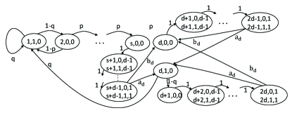
Figure 9: The threshold $s\leq d$ and the optimal decisions $\mu^{*}(1,1,0)=\mu^{*}(d,1,0)=1$.

Referring to Fig. 9, we derive the balance equations on the states $(2,0,0),(3,0,0),...,(s,0,0)$, and the $d-1$ combined states out of $(s,0,0)$ , and get

$$\begin{split}&\pi(s,0,0)=\pi(s+1,0,d-1)+\pi(s+d-1,1,d-1)\\ &...=\pi(s+d-1,0,1)+\pi(s+d-1,1,1),\\ &\pi(\delta,0,0)=(1-q)p^{\delta-2}\pi(1,1,0)\ \ \delta=2,3,...,s.\end{split}$$ (189)

We then observe the set $\{(1,1,0),(2,0,0),...,(s,0,0)\}$: the inflow of $q\pi(d,1,0)$ equals to the outflow $(s,0,0)$. Thus, combined with (LABEL:markov2_1),

$$q\pi(d,1,0)=\pi(s,0,0)=(1-q)p^{s-2}\pi(1,1,0).$$ (190)

The state $(d,1,0)$ gives

$$a_{d}\pi(d,0,0)=b_{d}\pi(s,0,0)+b_{d}(1-q)\pi(d,1,0),$$ (191)

thus,

$$\pi(d,0,0)=\frac{b_{d}}{a_{d}q}\pi(s,0,0)=\frac{b_{d}}{a_{d}q}(1-q)p^{s-2}\pi(1,1,0).$$ (192)

Thus, (LABEL:markov2_1), (190) and (192) imply that all the states in the Markov chain can be expressed in terms of $\pi(1,1,0)$. Also, the sums up of the probability of all the states is $1$:

$$\begin{split}&\pi(1,1,0)+\sum_{\delta=2}^{s}\pi(\delta,0,0)+(d-1)\pi(s,0,0)+d\pi(d,0,0)\\ &+(d(1-q)+1)\pi(d,1,0)=1.\end{split}$$ (193)

Thus,

$$\pi(1,1,0)=\frac{p}{(1-q)g_{2}(s)}.$$ (194)

Thus, we give the expected age to be $f_{2}(s)/g_{2}(s)$ in Table II.

P.3

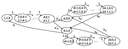
Figure 10: The threshold $s=1$ and the optimal decisions $\mu^{*}(1,1,0)=2,\mu^{*}(d,1,0)=1$.

Referring to Fig. 10, the $d-1$ combinations states from $(1,1,0)$ gives

$$\begin{split}&\pi(1,1,0)=\pi(2,0,d-1)+\pi(2,1,d-1)\\ &...=\pi(d,0,1)+\pi(d,1,1),\end{split}$$ (195)

the state $(1,1,0)$ gives

$$\pi(1,1,0)=q\pi(d,1,0).$$ (196)

Also,

$$\begin{split}&\pi(d+1,0,0)=\pi(d+2,0,d-1)+\pi(d+2,1,d-1)\\ &...=\pi(2d,0,1)+\pi(2d,1,1)=(1-q)\pi(d,1,0).\end{split}$$ (197)

The state of $(d,0,0)$ gives

$$(1-b_{d})\pi(d,0,0)=b^{\prime}_{d}\pi(1,1,0)+b_{d}\pi(d,1,0),$$ (198)

thus,

$$\pi(d,0,0)=\frac{b^{\prime}_{d}q+b_{d}}{1-b_{d}}\pi(d,1,0).$$ (199)

Thus, all state distributions can be expressed in terms of $\pi(d,1,0)$, and the expected age is $f_{0}/g_{0}$.

P.4

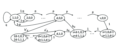
Figure 11: The threshold $s>d$ and the optimal decisions $\mu^{*}(1,1,0)=1,\mu^{*}(d,1,0)=2$.

Referring to Fig. 11, the states $(2,0,0),...,(d-1,0,0)$, $(d+1,0,0),...,(s,0,0)$, and $d-1$ states from $(s,0,0)$ give:

$$\begin{split}&\pi(\delta,0,0)=p^{\delta-2}(1-q)\pi(1,1,0)\ \ \delta=2,3,...,d-1,\\ &\pi(\delta,0,0)=p^{\delta-d}\pi(d,0,0)\ \ \delta=d+1,...,s,\\ &\pi(s,0,0)=\pi(s+1,0,d-1)+\pi(s+1,1,d-1)\\ &...=\pi(s+d-1,0,1)+\pi(s+d-1,1,1).\end{split}$$ (200)

The combination of states $(d,0,0)$ and $(d,1,0)$ gives

$$\pi(s,0,0)+p\pi(d-1,0,0)=\pi(d,0,0).$$ (201)

Equation (LABEL:markov4_1) implies that $\pi(d-1,0,0)=p^{d-3}(1-q)\pi(1,1,0)$, thus,

$$\pi(d,0,0)=\frac{p}{1-p^{s-d}}\pi(d-1,0,0)=\frac{p^{d-2}(1-q)}{1-p^{s-d}}\pi(1,1,0).$$ (202)

The state $(d,1,0)$ gives

$$\pi(d,1,0)(1-a^{\prime}_{d})=a_{d}\pi(s,0,0)=a_{d}p^{s-d}\pi(d,0,0).$$ (203)

Thus, all the states distributions in the Markov chain can be expressed in terms of $\pi(1,1,0)$. The expected age is $f_{3}(s)/g_{3}(s)$.

P.5

Figure 12: The threshold $s>d$ and the optimal decisions $\mu^{*}(1,1,0)=\mu^{*}(d,1,0)=2$.

Referring to Fig. 12, the balance equations of the $d-1$ states from $(s,0,0)$ and states $(d+1,0,0),...,(s,0,0)$ are given by:

$$\begin{split}&\pi(s,0,0)=\pi(s+1,0,d-1)+\pi(s+1,1,d-1)\\ &...=\pi(s+d-1,0,1)+\pi(s+d-1,1,1),\\ &\pi(\delta,0,0)=p^{\delta-d}\pi(d,0,0),\ \ \delta=d+1,...,s.\end{split}$$ (204)

The combination of $(d,0,0),(d,1,0)$ gives

$$\pi(1,1,0)+\pi(s,0,0)=\pi(d,0,0),$$ (205)

thus, using (LABEL:markov5_1), we get

$$\pi(1,1,0)=(1-p^{s-d})\pi(d,0,0).$$ (206)

By looking at $\pi(d,1,0)$,

$$(1-a^{\prime}_{d})\pi(d,1,0)=a_{d}\pi(s,0,0)+a^{\prime}_{d}\pi(1,1,0),$$ (207)

thus,

$$\pi(d,1,0)=\frac{a^{\prime}_{d}+(a_{d}-a^{\prime}_{d})}{1-a^{\prime}_{d}}\pi(d,0,0).$$ (208)

Thus, all the states distributions in the Markov chain can be expressed in terms of $\pi(d,0,0)$. Similar to previous sections, the distribution can be solved and the expected age is $f_{4}(s)/g_{4}(s)$.

P.6

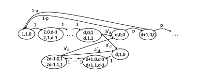
Figure 13: The optimal decisions $\mu^{*}(\delta,0,0)=1$ and $\mu^{*}(\delta,1,0)=2$ for all $\delta\geq 1$.

Referring to Fig. 13, the balance equations of the states $(d+1,0,0),...$ give

$$\pi(\delta,0,0)=p^{\delta-d}\pi(d,0,0)\ \ \delta=d+1,d+2,...$$ (209)

The state $(1,1,0)$ and the $d-1$ combinations states from $(1,1,0)$ imply that

$$\begin{split}&\pi(1,1,0)=\pi(2,0,d-1)+\pi(2,1,d-1)\\ &...=\pi(d,0,1)+\pi(d,1,1),\\ &\pi(1,1,0)=(1-p)\big{(}\pi(d,0,0)+\pi(d+1,0,0)+...\big{)}\end{split}$$ (210)

From (209),(210) we can get

$$\pi(1,1,0)=\pi(d,0,0).$$ (211)

The $d-1$ combinations states from $(d,1,0)$ implies that

$$\begin{split}&\pi(d,1,0)=\pi(d+1,0,d-1)+\pi(d+1,1,d-1)\\ &...=\pi(2d-1,0,1)+\pi(2d-1,1,1).\end{split}$$ (212)

The state $(d,1,0)$ gives

$$b^{\prime}_{d}\pi(1,1,0)+b^{\prime}_{d}\pi(d,1,0)=\pi(d,0,0).$$ (213)

thus,

$$\pi(d,1,0)=\frac{a^{\prime}_{d}}{b^{\prime}_{d}}\pi(d,0,0).$$ (214)

Thus, all the states probabilities can be expressed in terms of $\pi(d,0,0)$. By normalizing, we get $\pi(d,0,0)=1/g^{\prime}_{0}$. Then the expected age is $f^{\prime}_{0}/g^{\prime}_{0}$.

Appendix Q Proof of Lemma 14

We rewrite $\beta_{i}^{\prime}$:

$$\beta^{\prime}_{i} =\min_{s\in\{d+1,...\}}\frac{f_{i}(s)}{g_{i}(s)},\ i\in\{1,3,4\},$$ (215)

$$\beta^{\prime}_{2} =\min_{s\in\{1,...d\}}\frac{f_{2}(s)}{g_{2}(s)}.$$ (216)

Further, we rewrite (75) and (76):

$$h^{\prime}_{i}(c) =\min_{s\in\{d+1,...\}}f_{i}(s)-cg_{i}(s),\ i\in\{1,3,4\},$$ (217)

$$h^{\prime}_{2}(c) =\min_{s\in\{2,...d\}}f_{2}(s)-cg_{2}(s).$$ (218)

From Table II, it is easy to find that there exists a value $d^{\prime}>0$ such that $g_{i}(s)>d^{\prime}$ for all $s$ and $i$. Also, $g_{i}(s)$ is upper bounded. Thus, from (215),(216), (217) and (218), $h^{\prime}_{i}(c)\lesseqqgtr 0$ is equivalent to $c\gtreqqless\beta_{i}^{\prime}$, which proves our result.

Appendix R proof of Lemma 15

Notice that $(p,q,d)\in\textbf{B}_{2}\cup\textbf{B}_{3}$ if and only if $1-p<1/d$. Suppose that $r_{i}(c,s)\triangleq f_{i}(s)-cg_{i}(s)$.

We find that:

$$p^{-(s-1)}\Big{(}f_{i}(s+1)-f_{i}(s)\Big{)}=\Big{(}1-d(1-p)\Big{)}s+l^{\prime}_{i}$$ (219)

where $l^{\prime}_{i}$ is not related to $c,s$ and is described in Table II. Also,

$$p^{-(s-1)}\Big{(}g_{i}(s+1)-g_{i}(s)\Big{)}=o_{i},$$ (220)

where $o_{i}$ is not related to $c,s$ and are described in Table II as well. Thus, (219) and (220) give:

$$\begin{split}&p^{-(s-1)}(r_{i}(c,s+1)-r_{i}(c,s))\\ &=\Big{(}1-d(1-p)\Big{)}s+l^{\prime}_{i}-co_{i}.\end{split}$$ (221)

Note that (221) holds for $i\in\{1,2,3,4\}$. Since $1-(1-p)d>0$, (26) (for $i\in\{1,3,4\}$) and (27) (for $i=2$) are the minimum point of $r_{i}(c,s)$. Thus, we complete the proof.

References

- [1] J. Pan, A. M. Bedewy, Y. Sun, and N. B. Shroff, “Minimizing age of information via scheduling over heterogeneous channels,” in Proc. ACM MobiHoc, 2021, pp. 111–120.
- [2] R. D. Yates, Y. Sun, D. R. Brown, S. K. Kaul, E. Modiano, and S. Ulukus, “Age of information: An introduction and survey,” IEEE Journal on Selected Areas in Communications, vol. 39, no. 5, pp. 1183–1210, 2021.
- [3] S. Kaul, R. Yates, and M. Gruteser, “Real-time status: How often should one update?” in 2012 Proceedings IEEE INFOCOM, 2012, pp. 2731–2735.
- [4] M. Costa, M. Codreanu, and A. Ephremides, “On the age of information in status update systems with packet management,” IEEE Transactions on Information Theory, vol. 62, no. 4, pp. 1897–1910, 2016.
- [5] Y. Inoue, H. Masuyama, T. Takine, and T. Tanaka, “A general formula for the stationary distribution of the age of information and its application to single-server queues,” IEEE Transactions on Information Theory, vol. 65, no. 12, pp. 8305–8324, 2019.
- [6] B. Buyukates and S. Ulukus, “Age of information with Gilbert-Elliot servers and samplers,” in 2020 54th Annual Conference on Information Sciences and Systems (CISS), 2020, pp. 1–6.
- [7] A. M. Bedewy, Y. Sun, and N. B. Shroff, “Minimizing the age of information through queues,” IEEE Transactions on Information Theory, vol. 65, no. 8, pp. 5215–5232, 2019.
- [8] ——, “The age of information in multihop networks,” IEEE/ACM Transactions on Networking, vol. 27, no. 3, pp. 1248–1257, 2019.
- [9] Y. Sun, E. Uysal-Biyikoglu, and S. Kompella, “Age-optimal updates of multiple information flows,” in IEEE INFOCOM WKSHPS, 2018, pp. 136–141.
- [10] Y. Sun and B. Cyr, “Sampling for data freshness optimization: Non-linear age functions,” Journal of Communications and Networks, vol. 21, no. 3, pp. 204–219, 2019.
- [11] Y. Sun, Y. Polyanskiy, and E. Uysal, “Sampling of the Wiener process for remote estimation over a channel with random delay,” IEEE Transactions on Information Theory, vol. 66, no. 2, pp. 1118–1135, 2019.
- [12] A. M. Bedewy, Y. Sun, S. Kompella, and N. B. Shroff, “Optimal sampling and scheduling for timely status updates in multi-source networks,” IEEE Transactions on Information Theory, vol. 67, no. 6, pp. 4019–4034, 2021.
- [13] Y. P. Hsu, E. Modiano, and L. Duan, “Scheduling algorithms for minimizing age of information in wireless broadcast networks with random arrivals,” IEEE Transactions on Mobile Computing, vol. 19, no. 12, pp. 2903–2915, 2019.
- [14] R. Talak, S. Karaman, and E. Modiano, “Optimizing information freshness in wireless networks under general interference constraints,” IEEE/ACM Transactions on Networking, vol. 28, no. 1, pp. 15–28, 2019.
- [15] A. M. Bedewy, Y. Sun, R. Singh, and N. B. Shroff, “Low-power status updates via sleep-wake scheduling,” IEEE/ACM Transactions on Networking, 2021, in press.
- [16] C. Joo and A. Eryilmaz, “Wireless scheduling for information freshness and synchrony: Drift-based design and heavy-traffic analysis,” IEEE/ACM transactions on networking, vol. 26, no. 6, pp. 2556–2568, 2018.
- [17] N. Lu, B. Ji, and B. Li, “Age-based scheduling: Improving data freshness for wireless real-time traffic,” in Proc. ACM MobiHoc, 2018, pp. 191–200.
- [18] I. Kadota, A. Sinha, and E. Modiano, “Optimizing age of information in wireless networks with throughput constraints,” in Proc. IEEE INFOCOM, 2018, pp. 1844–1852.
- [19] Z. Qian, F. Wu, J. Pan, K. Srinivasan, and N. B. Shroff, “Minimizing age of information in multi-channel time-sensitive information update systems,” in IEEE INFOCOM 2020-IEEE Conference on Computer Communications, 2020, pp. 446–455.
- [20] Q. Liu, H. Zeng, and M. Chen, “Minimizing age-of-information with throughput requirements in multi-path network communication,” in Proc. ACM MobiHoc, 2019, pp. 41–50.
- [21] T. Z. Ornee and Y. Sun, “Sampling and remote estimation for the Ornstein-Uhlenbeck process through queues: Age of information and beyond,” IEEE/ACM Transactions on Networking, 2021, in press.
- [22] Y. Sun, E. Uysal-Biyikoglu, R. D. Yates, C. E. Koksal, and N. B. Shroff, “Update or wait: How to keep your data fresh,” IEEE Transactions on Information Theory, vol. 63, no. 11, pp. 7492–7508, 2017.
- [23] E. Altman, R. El-Azouzi, D. Menasche, and Y. Xu, “Forever young: Aging control for hybrid networks,” in Proc. ACM MobiHoc, 2019, pp. 91–100.
- [24] R. El-Azouzi, D. S. Menasche, Y. Xu et al., “Optimal sensing policies for smartphones in hybrid networks: A POMDP approach,” in 6th IEEE International ICST Conference on Performance Evaluation Methodologies and Tools, 2012, pp. 89–98.
- [25] R. Talak, S. Karaman, and E. Modiano, “Optimizing age of information in wireless networks with perfect channel state information,” in Proc. IEEE WiOpt, 2018, pp. 1–8.
- [26] “https://www.qualcomm.com/media/documents/files/vr-and-ar-pushing-connectivity-limits.pdf,” 2018.
- [27] T. S. Rappaport, S. Sun, R. Mayzus, H. Zhao, Y. Azar, K. Wang, G. N. Wong, J. K. Schulz, M. Samimi, and F. Gutierrez, “Millimeter wave mobile communications for 5G cellular: It will work!” IEEE access, vol. 1, pp. 335–349, 2013.
- [28] Samsung, 2018, https://news.samsung.com/us/verizon-samsung-reach-multi-gigabit-throughput-5g-nr-mmwave-spectrum/.
- [29] A. Narayanan, E. Ramadan, J. Carpenter, Q. Liu, Y. Liu, F. Qian, and Z. L. Zhang, “A first look at commercial 5G performance on smartphones,” in Proceedings of The Web Conference 2020, 2020, pp. 894–905.
- [30] Z. Pi and F. Khan, “An introduction to millimeter-wave mobile broadband systems,” IEEE communications magazine, vol. 49, no. 6, pp. 101–107, 2011.
- [31] ——, “System design and network architecture for a millimeter-wave mobile broadband (MMB) system,” in 34th IEEE Sarnoff Symposium, 2011, pp. 1–6.
- [32] O. Semiari, W. Saad, M. Bennis, and M. Debbah, “Integrated millimeter wave and sub-6 GHz wireless networks: A roadmap for joint mobile broadband and ultra-reliable low-latency communications,” IEEE Wireless Communications, vol. 26, no. 2, pp. 109–115, 2019.
- [33] D. Aziz, J. Gebert, A. Ambrosy, H. Bakker, and H. Halbauer, “Architecture approaches for 5G millimetre wave access assisted by 5G low-band using multi-connectivity,” in 2016 IEEE Globecom Workshops (GC Wkshps), 2016, pp. 1–6.
- [34] J. Deng, O. Tirkkonen, R. Freij-Hollanti, T. Chen, and N. Nikaein, “Resource allocation and interference management for opportunistic relaying in integrated mmWave/sub-6 GHz 5G networks,” IEEE Communications Magazine, vol. 55, no. 6, pp. 94–101, 2017.
- [35] H. Elshaer, M. N. Kulkarni, F. Boccardi, J. G. Andrews, and M. Dohler, “Downlink and uplink cell association with traditional macrocells and millimeter wave small cells,” IEEE Transactions on Wireless Communications, vol. 15, no. 9, pp. 6244–6258, 2016.
- [36] D. M. Topkis, Supermodularity and complementarity. Princeton university press, 1998.
- [37] V. Krishnamurthy, Partially observed Markov decision processes. Cambridge University Press, 2016.
- [38] M. L. Puterman, “Markov decision processes,” Handbooks in operations research and management science, vol. 2, pp. 331–434, 1990.
- [39] M. H. Ngo and V. Krishnamurthy, “Optimality of threshold policies for transmission scheduling in correlated fading channels,” IEEE Transactions on Communications, vol. 57, no. 8, pp. 2474–2483, 2009.
- [40] G. Yao, M. Hashemi, and N. B. Shroff, “Integrating sub-6 ghz and millimeter wave to combat blockage: delay-optimal scheduling,” in Proc. IEEE WiOpt, 2019, pp. 1–8.
- [41] D. P. Bertsekas, Dynamic programming and optimal control. Athena scientific Belmont, MA, 1995, vol. 1, no. 2.
- [42] L. I. Sennott, “Average cost optimal stationary policies in infinite state Markov decision processes with unbounded costs,” Operations Research, vol. 37, no. 4, pp. 626–633, 1989.
- [43] W. Dinkelbach, “On nonlinear fractional programming,” Management science, vol. 13, no. 7, pp. 492–498, 1967.
- [44] L. I. Sennott, “A new condition for the existence of optimal stationary policies in average cost Markov decision processes,” Operations research letters, vol. 5, no. 1, pp. 17–23, 1986.