DecAug: Out-of-Distribution Generalization via
Decomposed Feature Representation and Semantic Augmentation

Abstract

While deep learning demonstrates its strong ability to handle independent and identically distributed (IID) data, it often suffers from out-of-distribution (OoD) generalization, where the test data come from another distribution (w.r.t. the training one). Designing a general OoD generalization framework to a wide range of applications is challenging, mainly due to possible correlation shift and diversity shift in the real world. Most of the previous approaches can only solve one specific distribution shift, such as shift across domains or the extrapolation of correlation. To address that, we propose DecAug, a novel decomposed feature representation and semantic augmentation approach for OoD generalization. DecAug disentangles the category-related and context-related features. Category-related features contain causal information of the target object, while context-related features describe the attributes, styles, backgrounds, or scenes, causing distribution shifts between training and test data. The decomposition is achieved by orthogonalizing the two gradients (w.r.t. intermediate features) of losses for predicting category and context labels. Furthermore, we perform gradient-based augmentation on context-related features to improve the robustness of the learned representations. Experimental results show that DecAug outperforms other state-of-the-art methods on various OoD datasets, which is among the very few methods that can deal with different types of OoD generalization challenges.

Introduction

Deep learning has demonstrated superior performances on standard benchmark datasets from various fields, such as image classification (Krizhevsky, Sutskever, and Hinton 2012), object detection (Redmon et al. 2016), natural language processing (Devlin et al. 2019), and recommendation systems (Cheng et al. 2016), assuming that the training and test data are independent and identically distributed (IID). In practice, however, it is common to observe distribution shifts among training and test data, which is known as out-of-distribution (OoD) generalization. How to deal with OoD generalization is still an open problem.

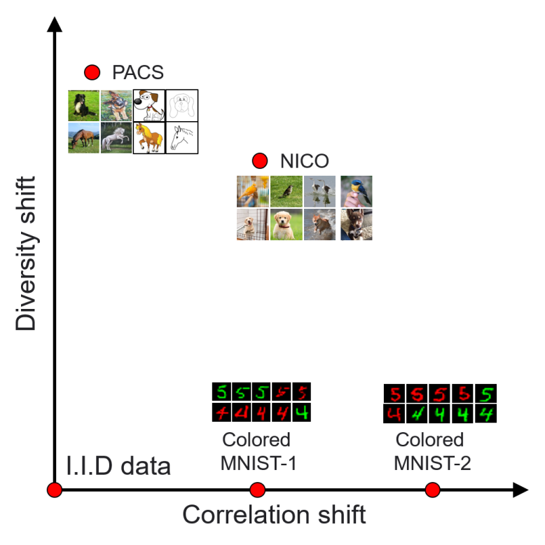
Figure 1: Illustration of the two-dimensional out-of-distribution problem among datasets in different OoD research areas, including Colored MNIST, PACS, and NICO. Extensive experiments showed that many OoD methods can only deal with one dimension of OoD generalization.

To improve a DNN’s OoD generalization ability, diversified research endeavours are observed recently, which mainly includes domain generalization, invariant risk minimization, and stable learning. Various standard benchmark datasets are adopted to evaluate the proposed OoD generalization algorithms, such as Colored MNIST (Arjovsky et al. 2019), PACS (Li et al. 2017a), and NICO (He, Shen, and Cui 2020). Among these datasets, PACS are widely used in domain generalization (Carlucci et al. 2019; Mancini et al. 2020) to validate DNN’s ability to generalize across different image styles. On the other hand, in recent risk regularization methods, Colored MNIST is often considered (Arjovsky et al. 2019; Ahuja et al. 2020; Krueger et al. 2020), where digits’ colors are either red or green. Manipulating the correlation between the colors and the labels would result in a distribution shift. In stable learning, another OoD dataset called NICO was introduced recently (He, Shen, and Cui 2020). It contains image style changes, background changes, and correlation extrapolation. Along with this dataset, an OoD learning method, named CNBB, is proposed, based on sample re-weighting inspired by causal inference.

In this paper, we observe that methods perform well in one OoD dataset, such as PACS, which may show very poor performance on another dataset, such as Colored MNIST, as shown in the our experiments. That may because of the different dimensions of OoD generalization. Here, we identify two types of out-of-distribution factors, including the correlation shift and the diversity shift.

Correlation shift. One is the correlation shift, which means that labels and the environments are correlated and the relations change across different environments. For example, in Fig. 2, we observe the correlation shift between the training set and the test set in Colored MNIST. Specifically, in the training set, number $5$ is usually in green while number $4$ is usually in red. However, in the test set, number $5$ tends to be in red while number $4$ tends to be in green. If a model learns color green to predict label $5$ when training, it would suffer from the correlation shift when testing.

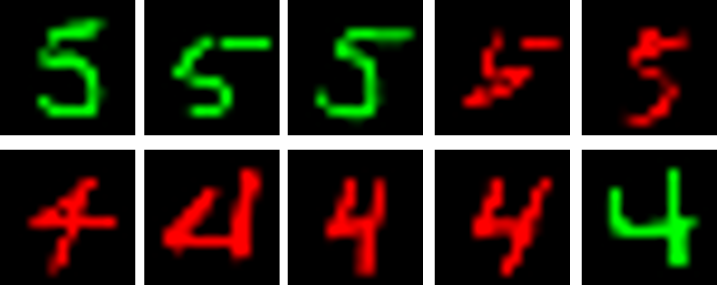
(a) Train

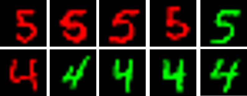
(b) Test

Figure 2: Typical examples of out-of-distribution correlation shift data from the Colored MNIST dataset.

Diversity shift. Another out-of-distribution factor is the diversity shift. For example, in PACS, the data come from four different domains: photo, art painting, cartoon and sketch. Data in different domains have significantly different styles. Usually, we leave one domain out as the test set, and the remaining three domains as training set. The model trained on the training set would susceptible to the diversity shift on the test set. See Fig. 3 as an illustration.

Two-dimension OoD. Data in actual scenarios usually involve two different OoD factors simultaneously. For example, in NICO (Fig. 4), different contexts such as “in cage”, “in water”, and “on grass” lead to diversity shift, while some contexts are related to specific categories, such as a bird would be “in hand” and a dog may be “at home”. We also put datasets from multiple research areas on the same axis (Fig. 1), the $X$-axis denotes the correlation shift which controls the contribution proportions of correlated features, the $Y$-axis denotes the diversity shift which stands for the change of feature types. Specifically, in the Colored MNIST dataset, the correlation between color and label is high, while in the PACS, the style of images is more diverse. In the NICO, both correlation shift and diversity shift exist.

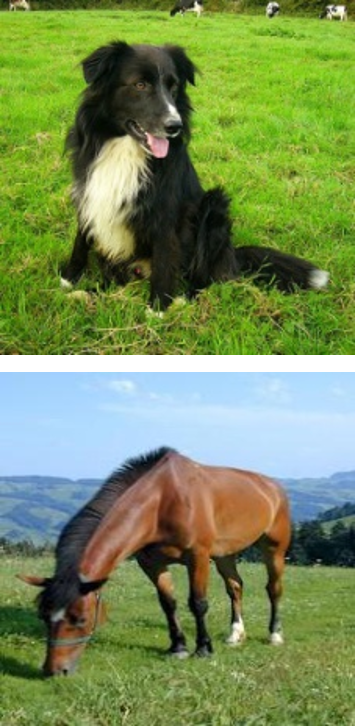
(a) P

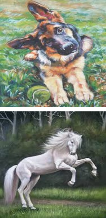
(b) A

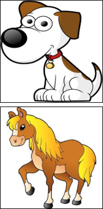
(c) C

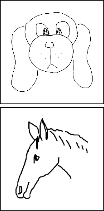
(d) S

Figure 3: Typical examples of out-of-distribution diversity shift data from the PACS dataset. (a) Photo. (b) Art Painting. (c) Cartoon. (d) Sketch.

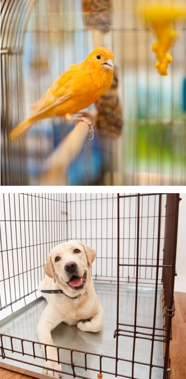
(a) In cage

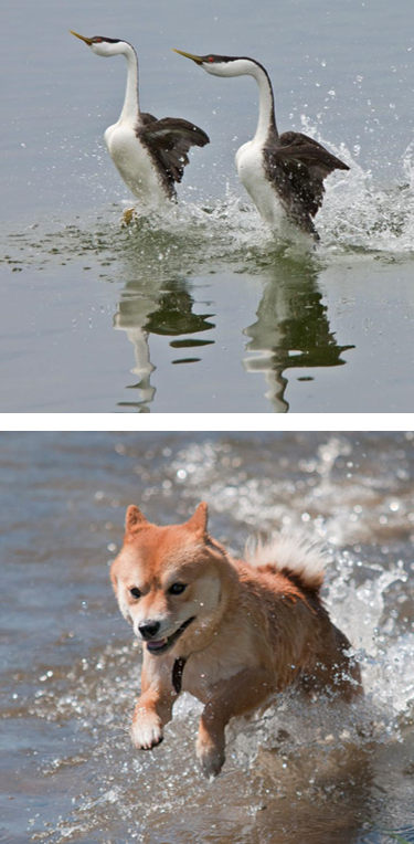
(b) In water

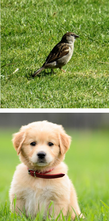
(c) On grass

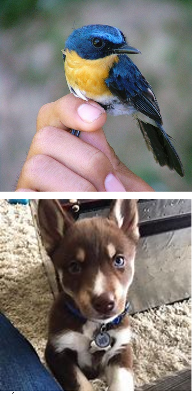
(d) Others

Figure 4: Some examples of the two-dimensional out-of-distribution data from the NICO dataset.

In our experiments, we showed that algorithms considered only one-dimension of OoD generalization may fail in the other dimension of OoD. To handle different OoD factors simultaneously, we propose DecAug, a novel decomposed feature representation and semantic augmentation approach for OoD generalization. Specifically, our method first decomposes the high-level representations of input images into category-related and context-related features by orthogonalizing the two gradients of losses for predicting category and context labels respectively. Category-related features are essential for recognizing the category labels of the images, while context-related features are not essential for the recognition but correlated with the category labels. After obtaining the decomposed features, we do gradient-based semantic augmentation on context-related features, representing attributes, styles, backgrounds, or scenes of target objects, to disentangle the spurious correlation between features that are not essential for the recognition and category labels.

Our contributions are as follows:

1. We test OoD methods from diversified research areas and show that very often, they only deal with one special type of OoD generalization challenge.

2. We propose DecAug to learn disentangled features that capture the information of category and context respectively and perform gradient-based semantic augmentation to enhance the generalization ability of the model. This is the first data augmentation method that attempts to deal with various OoD generalization problems indicating a new promising direction for OoD generalization.

3. Extensive experiments show that our method consistently outperforms previous OoD methods on various types of OoD tasks. For instance, we achieve an average accuracy of 82.39% with ResNet-18 (He et al. 2016) on PACS (Li et al. 2017a), which is the state-of-the-art performance.

Related Work

In this section, we review literature related to risk regularization methods, domain generalization, stable learning, data augmentation and disentangled representation.

Risk regularization methods for OoD generalization. The invariant risk minimization (IRM, (Arjovsky et al. 2019)) is motivated by the theory of causality and causal Bayesian networks (CBNs), aiming to find an invariant representation of data from different training environments. To make the model robust to unseen interventions, the invariant risk minimization added invariant risk regularization to monitor the optimality of a dummy classifier on different environments. IRM-Games (Ahuja et al. 2020) further improves the stability of IRM. Risk extrapolation (Rex, (Krueger et al. 2020)) adopts a min-max framework to derive a model that can perform well on the worst linear combination of risks from different environments. These methods typically perform well on synthetic datasets, such as Colored MNIST. However, it is unknown how they can generalize on more complex practical datasets beyond MNIST classification tasks.

Domain generalization. Fabio et al. proposed a self-supervised learning method—Jigsaw that achieves good performance in typical domain generalization datasets, such as PACS (Carlucci et al. 2019). A subnetwork sharing weights with the main network is used to solve Jigsaw puzzles. This self-supervised learning method helps in improving the generalization of model on unseen domains. Qi et al. adopted meta learning to learn invariant feature representations across domains (Dou et al. 2019). Recently, Mancini et al. proposed the curriculum mixup method for domain generalization, in which data from multiple domains in the training dataset mix together by a curriculum schedule of mixup method (Mancini et al. 2020). Domain generalization methods have achieved performance gain in generalizing models to unseen domains. However, recent OoD research finds that domain adaptation methods with similar design principles can have problems when training distribution is largely different from test distribution (Arjovsky et al. 2019).

Stable learning. Stable learning is a recently proposed new concept (Kuang et al. 2018), which focuses on learning a model that can achieve stable performances across different environments. The methodology of stable learning largely inherited from sampler reweighting in causal inference (Kuang et al. 2018; Shen et al. 2020; He, Shen, and Cui 2020). For example, in the convnets with batch balancing algorithm (CNBB), instead of viewing all samples in the dataset equally, it first calculates the weights of each sample by a confounder balancing loss which tests whether including or excluding a sample’s feature can lead to a significant change in the latent feature representations to reduce the effects of samples that are largely affected by confounders (Imai and Ratkovic 2014; Robins, Rotnitzky, and Zhao 1994). While these methods can have theoretical guarantees on simplified models, when confounder results in strong spurious correlations, this method may not be able to work well especially in the deep learning paradigm.

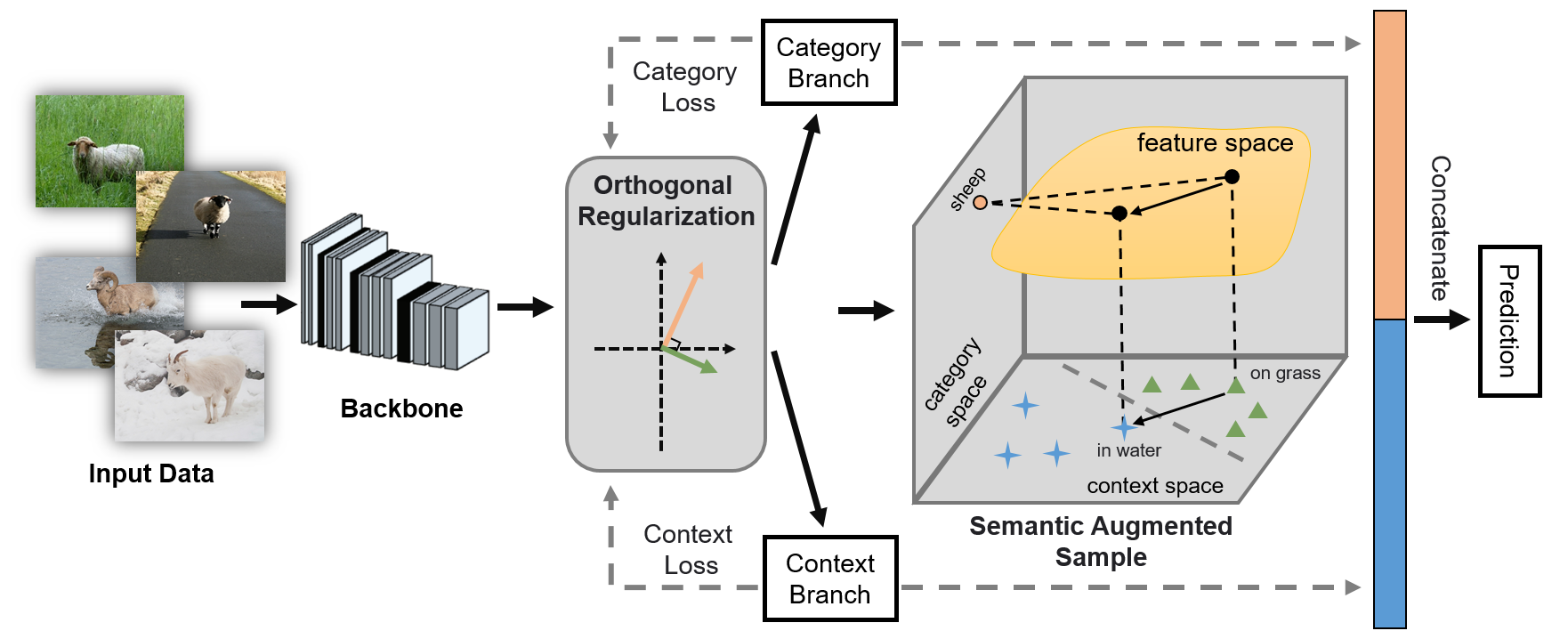
Figure 5: An overview of the proposed DecAug. The input features $z$ extracted by the backbone are decomposed into category-related and context-related features with orthogonal regularization. Gradient-based augmentation is then preformed in the feature space to get semantic augmented samples.

Data augmentation. Data augmentation has been widely used in deep learning to improve the generalization ability of deep models (Krizhevsky, Sutskever, and Hinton 2012; Srivastava, Greff, and Schmidhuber 2015; Han, Kim, and Kim 2017). Elaborately designed augmentation strategies, such as Cutout (DeVries and Taylor 2017), Mixup (Zhang et al. 2017), CutMix (Yun et al. 2019), and AugMix (Hendrycks et al. 2019), have effectively improved the performance of deep models. A more related augmentation method is to interpolate high-level representations. Upchurch et al. (2017) shows that simple linear interpolation can achieve meaningful semantic transformations. Motivated by this observation, Wang et al. (2019) proposes to augment deep features with random vectors sampled from class-specific normal distributions. Instead of augmenting the features explicitly, they minimize an upper bound of the expected loss on augmented data. To tackle few-shot learning problem, Hariharan and Girshick (2017) suggest to train a feature generator that can transfer modes of variation from categories of a large dataset to novel classes with limited samples. To ease the learning from long-tailed data, Liu et al. (2020a) proposes to transfer the intra-class distribution of head classes to tail classes by augmenting deep features of instances in tail classes. Different from these approaches, our method performs gradient-based augmentation on disentangled context-related features to eliminate distribution shifts for various OoD tasks.

Disentangled representation. Disentangling the latent factors from the image variants is a promising way to provide an understanding of the observed data (Chen et al. 2016; Higgins et al. 2017; Ma et al. 2019). It aims to learn representations that separate the explanatory factors of variations behind the data. Such representations are more resilient to the complex variants and able to bring enhanced generalization ability (Liu et al. 2018; Peng et al. 2019). Disentangled representations are inherently more interpretable. How to obtain disentanglement is still a challenging problem. Shen and Zhou (2020) identifies latent semantics and examines the representation learned by GANs. It derives a closed-form factorization method to discover latent semantic and prove that all semantic directions found are orthogonal in the latent space. Bahng et al. (2020) trains a de-biased representation by encouraging it to be different from a set of representations that are biased by design. The method discourages models from taking bias shortcuts, resulting in improved performances on de-biased test data. In this paper, semantic vectors found by DecAug with orthogonal constraints are disentangled from each other in the feature space.

Methodology

To deal with the aforementioned two different types of distribution shifts simultaneously, we argue that it is critical to obtain the decomposed features, one is essential for predicting category and the other is not essential but correlated for recognition. In this section, we propose DecAug to learn decomposed high-level representations for the input data. The decomposition is achieved by orthogonalizing the two gradients of losses for predicting category and context labels respectively. To improve the generalization ability, we perform gradient-based semantic augmentation on context-related features and concatenate the augmented features to category-related features to make the final prediction. An overview of the proposed method is illustrated in Fig. 5.

Feature Decomposition

Consider an image recognition task with the training set $\mathcal{D}=\{(x_{i},y_{i},c_{i})\}_{i=1}^{N}$, where $x_{i}$ is the input image, $y_{i}$ is the corresponding category label, $c_{i}$ is the corresponding context label, and $N$ is the number of training data. As shown in Fig. 5, the input data are mapped to the feature space and are decomposed into two branches: category branch and context branch. Given an input image $x_{i}$ with category label $y_{i}$ and context label $c_{i}$, let $z_{i}=g_{\theta}(x_{i})$ be the features extracted by a backbone $g_{\theta}$. For the category branch, $z_{i}$ is decomposed into $z^{1}_{i}=f_{\theta^{1}}(z_{i})$ by a category feature extractor $f_{\theta^{1}}$, followed by a classifier $h_{\phi^{1}}(z^{1}_{i})$ to predict the category label. For the context branch, $z_{i}$ is decomposed into $z^{2}_{i}=f_{\theta^{2}}(z_{i})$ by a context feature extractor $f_{\theta^{2}}$, followed by a classifier $h_{\phi^{2}}(z^{2}_{i})$ to predict the context label. We use the standard cross-entropy losses $\mathcal{L}^{1}_{i}(\theta,\theta^{1},\phi^{1})=\ell(h_{\phi^{1}}\circ f_{\theta^{1}}(z_{i}),y_{i})$ and $\mathcal{L}^{2}_{i}(\theta,\theta^{2},\phi^{2})=\ell(h_{\phi^{2}}\circ f_{\theta^{2}}(z_{i}),c_{i})$ to optimize these two branches, together with the backbone, respectively.

Algorithm 1 DecAug: Decomposed Feature Representation and Semantic Augmentation for OoD generalization

0:  Training set $\mathcal{D}$, batch size $n$, learning rate $\beta$, hyper-parameters $\epsilon$, $\lambda^{1}$, $\lambda^{2}$, $\lambda^{\text{orth}}$.

0:  $\theta$, $\theta^{1}$, $\phi^{1}$, $\theta^{2}$, $\phi^{2}$, $\phi$.

1:  Initialize $\theta$, $\theta^{1}$, $\phi^{1}$, $\theta^{2}$, $\phi^{2}$, $\phi$;

2:  repeat

3:     Sample a mini-batch of training images $\{(x_{i},y_{i},c_{i})\}_{i=1}^{n}$ with batch size $n$;

4:     for each $(x_{i},y_{i},c_{i})$ do

5:        $z_{i}\leftarrow g_{\theta}(x_{i})$;

6:        $\mathcal{L}^{1}_{i}(\theta,\theta^{1},\phi^{1})\leftarrow\ell(h_{\phi^{1}}\circ f_{\theta^{1}}(z_{i}),y_{i})$;

7:        $\mathcal{L}^{2}_{i}(\theta,\theta^{2},\phi^{2})\leftarrow\ell(h_{\phi^{2}}\circ f_{\theta^{2}}(z_{i}),c_{i})$;

8:        Compute $\mathcal{L}^{\text{orth}}_{i}(\theta^{1},\phi^{1},\theta^{2},\phi^{2})$ according to Eq. (1);

9:        Randomly sample $\alpha_{i}$ from $[0,1]$;

10:        Generate $\tilde{z}^{2}_{i}$ according to Eq. (2);

11:        $\mathcal{L}^{\text{concat}}_{i}(\theta,\theta^{1},\theta^{2},\phi)\leftarrow\ell(h_{\phi}([f_{\theta^{1}}(z_{i}),\tilde{z}^{2}_{i}]),y_{i})$;

12:        Compute $\mathcal{L}_{i}(\theta,\theta^{1},\phi^{1},\theta^{2},\phi^{2},\phi)$ according to Eq. (3);

13:     end for

14:     $(\theta,\theta^{1},\phi^{1},\theta^{2},\phi^{2},\phi)\leftarrow(\theta,\theta^{1},\phi^{1},\theta^{2},\phi^{2},\phi)$ $-\beta\cdot\nabla\frac{1}{n}\sum\limits_{i=1}^{n}\mathcal{L}_{i}(\theta,\theta^{1},\phi^{1},\theta^{2},\phi^{2},\phi)$;

15:  until convergence;

It is known that the direction of the non-zero gradient of a function is the direction in which the function increases most quickly, while the direction that is orthogonal to the gradient direction is the direction in which the function increases most slowly. To better decompose the features into category-related and context-related features, we enforce the gradient of the category loss $\ell(h_{\phi^{1}}\circ f_{\theta^{1}}(z_{i}),y_{i})$ to be orthogonal to the gradient of the context loss $\ell(h_{\phi^{2}}\circ f_{\theta^{2}}(z_{i}),c_{i})$ with respect to $z_{i}$, such that the direction that changes the category loss most quickly will not change the context loss from $z_{i}$ and vice versa. Specifically, let $\mathcal{G}^{1}_{i}(\theta^{1},\phi^{1})=\nabla_{z_{i}}\ell(h_{\phi^{1}}\circ f_{\theta^{1}}(z_{i}),y_{i})$ and $\mathcal{G}^{2}_{i}(\theta^{2},\phi^{2})=\nabla_{z_{i}}\ell(h_{\phi^{2}}\circ f_{\theta^{2}}(z_{i}),c_{i})$ be the gradients of the category and context loss with respect to $z_{i}$ respectively. To ensure the orthogonality, we minimize the following loss:

$$\mathcal{L}^{\text{orth}}_{i}(\theta^{1},\phi^{1},\theta^{2},\phi^{2})=(\frac{\mathcal{G}^{1}_{i}(\theta^{1},\phi^{1})}{\left\lVert\mathcal{G}^{1}_{i}(\theta^{1},\phi^{1})\right\rVert}\cdot\frac{\mathcal{G}^{2}_{i}(\theta^{2},\phi^{2})}{\left\lVert\mathcal{G}^{2}_{i}(\theta^{2},\phi^{2})\right\rVert})^{2}.$$ (1)

Semantic Augmentation

Considering that context-related features cause correlation or diversity shifts in our setting, we perform augmentation on the context-related features to eliminate such kind of distribution shifts. As in the semantic feature space, we may have multiple alternative directions for OoD. To ensure good performances across different environments, we postulate a worse case for the model to learn for OoD generalization by calculating the adversarially perturbed examples in the feature space. Specifically, let $\mathcal{G}^{\text{aug}}_{i}=\nabla_{z^{2}_{i}}\ell(h_{\phi^{2}}(z^{2}_{i}),c_{i})$ be the gradient of the context loss with respect to $z^{2}_{i}$. We augment the context-related features $z^{2}_{i}$ as follows:

$$\tilde{z}^{2}_{i}=z^{2}_{i}+\alpha_{i}\cdot\epsilon\cdot\frac{\mathcal{G}^{\text{aug}}_{i}}{\left\lVert\mathcal{G}^{\text{aug}}_{i}\right\rVert},$$ (2)

where $\epsilon$ is a hyper-parameter that determines the maximum length of the augmentation vectors and $\alpha_{i}$ is randomly sampled from $[0,1]$.

After augmenting the context-related features, we concatenate $\tilde{z}^{2}_{i}$ to the category-related features $z^{1}_{i}$ to make the final prediction $h_{\phi}([z^{1}_{i},\tilde{z}^{2}_{i}])$, where $h_{\phi}$ is a classifier and $[z^{1}_{i},\tilde{z}^{2}_{i}]$ is the concatenation of two features. We still use the standard cross-entropy loss $\mathcal{L}^{\text{concat}}_{i}(\theta,\theta^{1},\theta^{2},\phi)=\ell(h_{\phi}([z^{1}_{i},\tilde{z}^{2}_{i}]),y_{i})$ to optimize the corresponding parameters. Together with the aforementioned losses, the final loss is then defined as

$$\mathcal{L}_{i}(\theta,\theta^{1},\phi^{1},\theta^{2},\phi^{2},\phi) =\mathcal{L}^{\text{concat}}_{i}(\theta,\theta^{1},\theta^{2},\phi)$$ (3)

$$+\lambda^{1}\cdot\mathcal{L}^{1}_{i}(\theta,\theta^{1},\phi^{1})+\lambda^{2}\cdot\mathcal{L}^{2}_{i}(\theta,\theta^{2},\phi^{2})$$

$$+\lambda^{\text{orth}}\cdot\mathcal{L}^{\text{orth}}_{i}(\theta^{1},\phi^{1},\theta^{2},\phi^{2}),$$

where $\lambda^{1}$, $\lambda^{2}$ and $\lambda^{\text{orth}}$ are hyper-parameters that balance different losses. We formulate the learning of DecAug as the following optimization problem:

$$\min_{\theta,\theta^{1},\phi^{1},\theta^{2},\phi^{2},\phi}\,\frac{1}{N}\sum_{i=1}^{N}\mathcal{L}_{i}(\theta,\theta^{1},\phi^{1},\theta^{2},\phi^{2},\phi).$$ (4)

The stochastic gradient descent (SGD) algorithm can be applied to optimize the above objective. The detailed procedures are summarized in Algorithm 1.

Experiments

In this section, we will conduct numerical experiments to cross benchmark different methods from different perspective of OoD research on different typically challenging and widely used dataset–Colored MNIST, NICO, and PACS.

Implementation Details and Datasets

We evaluate our method on three challenging OoD datasets with different levels of correlation shift and diversity shift as discussed above: Colored MNIST (Arjovsky et al. 2019), PACS (Li et al. 2017a), and NICO (He, Shen, and Cui 2020). The main task of DecAug is category classification subject to unseen data distributions. For PACS and Colored MNIST, the context labels are domain/environment IDs. For NICO, it is attributes. The metric is the top-1 category classification accuracy.

The Colored MNIST Dataset. The challenging Colored MNIST dataset was recently proposed by IRM (Arjovsky et al. 2019) via modifying the original MNIST dataset with three steps: 1) The original digits ranging from 0 to 4 were relabelled as 0 and the digits ranging from 5 to 9 were tagged as 1; 2) The labels of 0 have a probability of $25\%$ to flip to 1, and vice versa; 3) The digits were colored either red or green based on different correlation with the labels to construct different environments (e.g., $80\%$ and $90\%$ for the training environments and $10\%$ for the test environment). In this way, the classifiers will easily over-fit to the spurious feature (e.g., color) in the training environments and ignore the shape feature of the digits.

For a fair comparison, we followed the same experimental protocol as in IRM (Arjovsky et al. 2019) on the Colored MNIST dataset. We equipped the IRMv1 scheme with our DecAug approach using the same settings. The backbone network was a three-layer MLP. The total training epoch was 500 and the batch size was the whole training data. We used the SGD optimizer with an initial learning rate of 0.1. The trained model was tested at the final epoch.

The PACS Dataset. This dataset contains 4 domains (Photo, Art Painting, Cartoon, Sketch) with 7 common categories (dog, elephant, giraffe, guitar, horse, house, person). We followed the same leave-one-domain-out validation experimental protocol as in  (Li et al. 2017a). For each time, we select three environments for training and the remaining environment for testing.

The backbone network we used on PACS dataset was ResNet-18. We followed the same training, validation and test split as in JiGen (Carlucci et al. 2019). The number of training epochs was 100. The batch size was 64. We used the SGD optimizer with a learning rate of 0.02.

The NICO Dataset. This dataset contains 19 classes with 9 or 10 different contexts, i.e., different object poses, positions, backgrounds, and movement patterns, etc. The NICO dataset is one of the newly proposed OoD generalization benchmark in the real scenarios (He, Shen, and Cui 2020). The contexts in validation and test set will not appear in training set.

The backbone network was ResNet-18 without pretraining on the NICO dataset. The number of training epochs was 500 and the batch size was 128. We used the SGD optimizer with a learning rate of 0.05.

We compare our proposed DecAug with the state-of-the-arts, including empirical risk minimization (ERM), invariant risk minimization (IRM, (Arjovsky et al. 2019)), invariant risk minimization games (IRM-Games, (Ahuja et al. 2020)), model-agnostic learning of semantic features (MASF, (Dou et al. 2019)), domain generalization by solving jigsaw puzzles (JiGen, (Carlucci et al. 2019)) across multiple datasets, debiased training method (ReBias, (Bahng et al. 2020)), risk extrapolation (Rex, (Krueger et al. 2020)), and convnets with batch balancing (CNBB, (He, Shen, and Cui 2020)).

Our framework was implemented with PyTorch 1.1.0, CUDA v9.0. For the baseline methods, we implement either with Pytorch 1.1.0 or with Tensorflow 1.8 to keep the same setting as their original source code. IRM, JiGen, ReBias, Rex, and CNBB were implemented with Pytorch. IRM-Games and MASF were implemented with Tensorflow. We conducted experiments on NVIDIA Tesla V100. More implementation details can be found in the Appendix.

Results and Discussion

In this section, we evaluate and analyze the results of our approach on three datasets: Colored MNIST, PACS and NICO. These datasets represent different aspects of covariant shifts in OoD problems thus provide more thorough studies on OoD generalization compared with previous ones.

Table 1: Classification accuracy of our approach trained considering leave-one-domain-out validation compared with the state-of-the-art methods on the PACS benchmark with the ResNet-18 backbone.

Model Art Painting Cartoon Sketch Photo Average ERM (Carlucci et al. 2019) 77.85 74.86 67.74 95.73 79.05 IRM (Arjovsky et al. 2019)^* 70.31 73.12 75.51 84.73 75.92 Rex (Krueger et al. 2020)^* 76.22 73.76 66.00 95.21 77.80 JiGen (Carlucci et al. 2019) 79.42 75.25 71.35 96.03 80.51 DANN (Ganin et al. 2016) 81.30 73.80 74.30 94.00 80.80 MLDG (Li et al. 2017b) 79.50 77.30 71.50 94.30 80.70 CrossGrad (Shankar et al. 2018) 78.70 73.30 65.10 94.00 80.70 MASF (Dou et al. 2019) 80.29 77.17 71.69 94.99 81.03 Cumix (Mancini et al. 2020) 82.30 76.50 72.60 95.10 81.60 DecAug 79.00 79.61 75.64 95.33 82.39 * Implemented by ourselves.

Table 2: Results of our approach compared with different methods on the Colored MNIST dataset(mean $\pm$ std deviation).

Model Acc test env ERM^* 17.10 $\pm$ 0.6 IRM (Arjovsky et al. 2019) 66.90 $\pm$ 2.5 Rex (Krueger et al. 2020) 68.70 $\pm$ 0.9 F-IRMGames (Ahuja et al. 2020) 59.91 $\pm$ 2.7 V-IRMGames (Ahuja et al. 2020) 49.06 $\pm$ 3.4 ReBias (Bahng et al. 2020)^* 29.40 $\pm$ 0.3 JiGen (Carlucci et al. 2019)^* 11.91 $\pm$ 0.4 DecAug 69.60 $\pm$ 2.0 ERM, grayscale model(oracle) 73.00 $\pm$ 0.4 Optimal invariant model (hypothetical) 75.00 * Implemented by ourselves.

Illustrative Results on the Colored MNIST Dataset. As shown in Table 2, DecAug achieves the best generalization performance on Colored MNIST, followed by risk regularization methods, such as Rex and IRM. For typical domain generalization methods, such as JiGen, and the recently proposed method ReBias, are misled by the spurious correlation existing in the training datasets. Notice that DecAug’s performance is very close to ERM trained on grayscale MNIST which provides an upper bound for MLP to generalize on this task. As mentioned in (Arjovsky et al. 2019), typical domain generalization methods can only deal with one dimension of OoD problem where image style differs. Our method further improves the performance in Colored MNIST by decomposition and semantic augmentation in the feature space, which disregards spurious features that are correlated but not causal for predicting category.

Table 3: Results of our method compared with different models on the NICO dataset.

Model Animal Vehicle ERM^* 75.87 74.52 IRM (Ahuja et al. 2020)^* 59.17 62.00 Rex (Krueger et al. 2020)^* 74.31 66.20 Cumix (Mancini et al. 2020)^* 76.78 74.74 DANN (Ganin et al. 2016)^* 75.59 72.23 JiGen (Carlucci et al. 2019)^* 84.95 79.45 CNBB (He, Shen, and Cui 2020)^* 78.16 77.39 DecAug 85.23 80.12 * Implemented by ourselves.

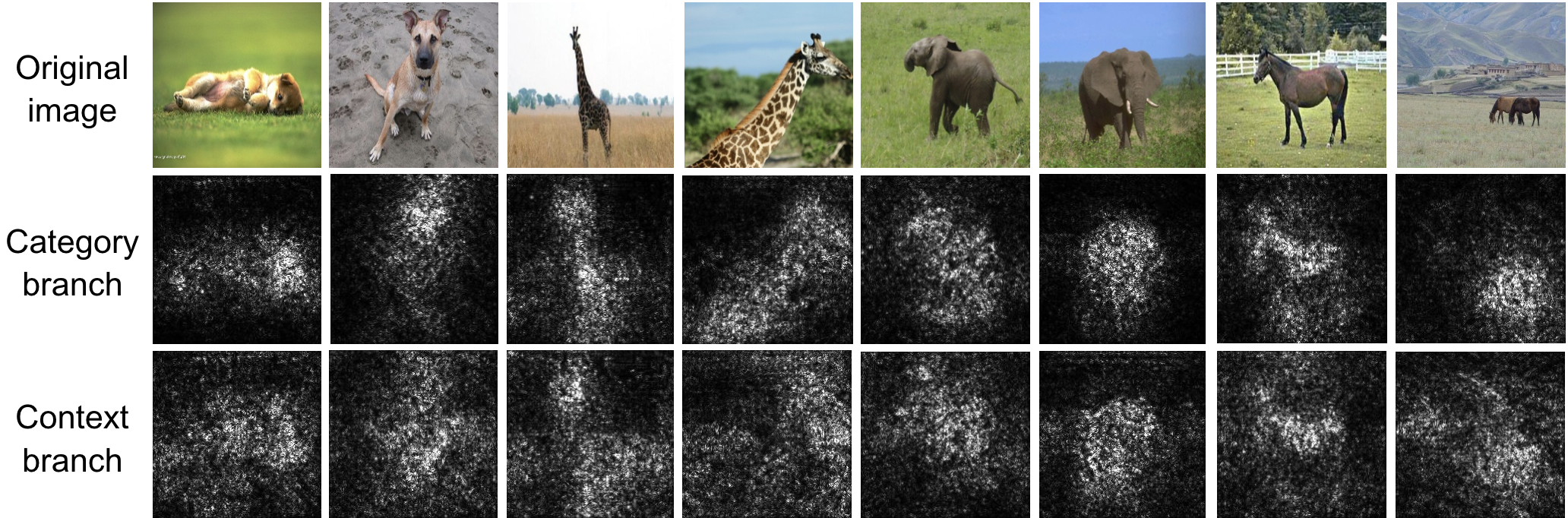
Figure 6: The gradient visualization of the decomposed category-related and context-related high-dimensional features. The first row is the original input images, the second row is its corresponding back propagation of the category branch and the last row is the back propagation of the context branch.

Illustrative Results on the PACS Dataset. In PACS, DecAug achieves the state-of-the-art (SOTA) performance followed by MASF and Cumix when using ResNet-18 as the backbone network. The details of our results on PACS are shown in Table 1. The worse performances for risk regularization methods, such as IRM and Rex, are because these methods add strong regularization terms in ERM to eliminate all features that are unstable across different environments. This can work well in the standard and “clean” dataset—-MNIST, where shapes of digits are always stable. However, in realistic scenarios, the shapes of target objects can change, meaning that even features for predicting object category can be unstable in different training environments.

Illustrative Results on the NICO Dataset. The recently proposed NICO dataset, considers more realistic generalization scenarios, where objects themselves and the backgrounds i.e.contexts in the dataset, can change vastly. For example, in the training dataset, we have dog pictures on the grass with dog faces posed to the camera, while in the test dataset, there are pictures where dogs are moving on the beachside. In our implementation, CuMix achieved 76.78% (animal) and 74.74% (vehicle) accuracy on NICO, indicating that mixing up (interpolating) data may not able to correct the spurious correlation between irrelevant features such as the background to the predicted category. In addition, DANN achieved 64.77% (animal) and 58.16% (vehicle) accuracy, which is similar to IRM. The poor performance of DANN and IRM on NICO may probably due to the diversity shift. As Table 3 shows, the proposed DecAug achieved the best generalization performances on two sets, followed by JiGen. This further demonstrates the superiority of the proposed algorithmic framework. Our method has achieved the SOTA performance simultaneously on various OoD generalization tasks, indicating a new promising direction for OoD learning algorithm research.

Table 4: Ablation study on PACS with ResNet-18.

PACS Art Painting Cartoon Sketch Photo Average DecAug without orth loss 78.42 78.32 72.13 94.19 80.77 DecAug (orth 0.0005) 77.49 77.43 74.32 94.07 80.76 DecAug (orth 0.001) 78.12 77.34 76.97 94.91 81.83 DecAug (orth 0.01) 79.00 79.61 75.64 95.33 82.39

Ablation Studies and Sensitivity Analysis

For ablation studies and sensitivity analysis, we take the PACS dataset for example.

Effectiveness of orthogonal loss. We test the effects of the proposed orthogonal loss. The results are shown in Table 4. It can be seen that without the orthogonal loss, our method achieves the average accuracy of 80.77% that is higher than most of the methods in Table 1. This is because the category and context losses also play the role of feature decomposition. The additional orthogonal loss enforces the gradients of the category and context losses to be orthogonal to each other, which helps to further decompose the features. As expected, with the increase of the orthogonal regularization coefficient $\lambda^{\text{orth}}$, the performance of DecAug can be improved. The experimental results confirm the effectiveness of the proposed orthogonal loss.

DecAug variants. We changed current orth regularization to orth constrains between features, refer to Table 5, which reaches 79.90% on PACS, lower than the original DecAug. We also tried confusion regularization, as discussed in recent literature Open Compound Domain Adaptation (Liu et al. 2020b). It seems natural to incorporate confusion regularization into our method for better decomposition. However, after many trials, no improvements were observed. We tried DecAug with DANN adversarial loss ”orth” on PACS. As shown in Table 5, the result is around 81%, lower than the original. This shows both gradient orthogonalization and semantic augmentation are both indispensable parts in the algorithm. We tried ”adversarial augmentation” to Jigsaw, the result is much lower than Jigsaw. This shows that the two branch architecture is needed and adversarial augmentation is better performed on the context predicting branch to improve OoD generalization via challenging neural networks to unseen context information.

Table 5: Results of DecAug variants on the PACS dataset.

Model Average DecAug (DANN loss) 81.00 DecAug (orth between features) 79.90 DecAug (gradient-based orth) 82.39

Interpretability analysis. We also use deep neural network interpretability methods in (Adebayo et al. 2018) to explain the neural network’s classification decisions as shown in Figure 6. It can be seen that the saliency maps of the category branch focus more on foreground objects, while the saliency maps of the context branch are also sensitive to background contexts that contain domain information. This shows that our method well decomposes the high-level representations into two features that contain category and context information respectively. Later, by performing semantic augmentation on context-related features, our model breaks the inherent relationship between contexts and category labels and generalizes to unseen combinations of foregrounds and backgrounds.

Conclusions

In this paper, we propose DecAug, a novel decomposed feature representation and semantic augmentation method for various OoD generalization tasks. High-level representations for the input data are decomposed into category-related and context-related features to deal with the diversity shift between training and test data. Gradient-based semantic augmentation is then performed on the context-related features to break the spurious correlation between context features and image categories. To the best of our knowledge, this is the first method that can simultaneously achieve the SOTA performance on various OoD generalization tasks from different research areas, indicating a new research direction for OoD generalization research. For future work, we will construct a large OoD dataset from the industry to further improve the algorithm and put it into real practice.

Appendix A Supplementary Materials

Ablation Study for Semantic Augmentation

In DecAug, semantic augmentation is proposed to further alleviate the influence of spurious correlation. We do not use random noise but adversarial augmentation on the context branch to improve the generalization ability of the model. In this section, we investigate the effects of semantic augmentation. We follow the same leave-one-domain-out validation protocol and the same training, validation and test split as in Li et al. (2017a). The maximum number of training epochs in our experiment is 100. We use the SGD optimizer with a batch size of 64. Recall that $\epsilon$ is the magnitude of perturbation in augmentation. We test different values of $\epsilon$ when all the other hyper-parameters remain the same. The results are summarized in Table 6. The first row lists the performance of the baseline model without augmentation. As can be seen in rows 2 and 4, semantic augmentation significantly improves classification accuracy. DecAug without semantic augmentation achieves $79.64\%$ accuracy, which is lower than DecAug. This is because semantic augmentation uses adversarial perturbation on the semantic space for improving the robustness of DecAug to unseen semantic domains. Moreover, the magnitude of the perturbation has a great influence on the results. Inappropriate magnitudes of perturbation would lead to very poor performance.

Table 6: Ablation study for semantic augmentation on PACS with ResNet-18.

PACS Art Painting Cartoon Sketch Photo Average DecAug without perturbation 75.83 77.37 70.81 94.55 79.64 DecAug ($\epsilon=1$) 79.00 79.61 75.64 95.33 82.39 DecAug ($\epsilon=0.01$) 75.24 77.65 69.89 94.67 79.36 DecAug ($\epsilon=10$) 74.39 77.47 75.24 95.09 80.55 DecAug ($\epsilon=100$) 63.13 70.39 64.19 94.55 73.07 DecAug ($\epsilon=1000$) 62.89 71.97 71.44 41.13 61.86

Ablation Study for Features Concatenation

In this section, we conduct an ablation study for features concatenation. Following the same leave-one-domain-out validation protocol as in the previous works on PACS, we evaluate the proposed DecAug without the concatenate operation. The balance weight for the category branch and the context branch is one. Note that we also involve the orthogonal constraints in this experiment. As can be seen in Table 7, the application of features concatenation achieves the best performance.

Table 7: Ablation study for features concatenate on PACS with ResNet-18.

PACS Art Painting Cartoon Sketch Photo Average DecAug with concat 79.00 79.61 75.64 95.33 82.39 DecAug without concat 75.83 76.24 75.57 94.79 80.61

Gradient Visualization of DecAug in NICO

We use deep neural network interpretation methods to explain the neural network’s classification decisions in NICO, as shown in Figure 7. It can be seen that the saliency maps of the category branch focus more on foreground objects, while the saliency maps of the context branch are also sensitive to background contexts that contain domain information.

Experimental Details of NICO

The NICO dataset contains two superclasses: animal and vehicle, which is a newly proposed OoD generalization benchmark in the real world. The original NICO dataset describes different ways to split training, validation and test set. For a fair comparison, we fix the split settings and constrain that the contexts have no intersection among the training, validation and test sets. The details of the split principle used in our experiments are shown in Table 8 and Table 9.

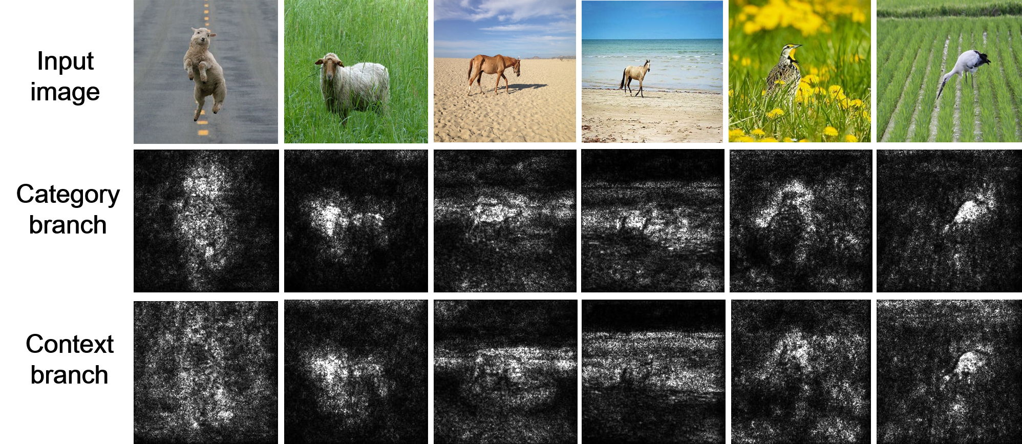
(a) Animal

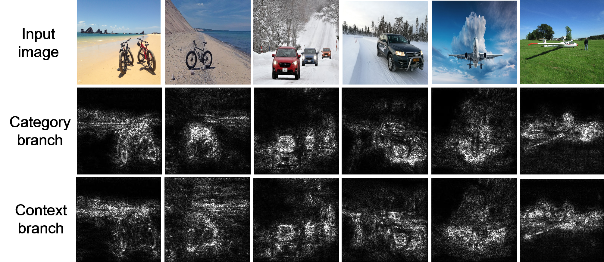
(b) Vehicle

Figure 7: The gradient visualization of the decomposed category-related and context-related high-dimensional features in NICO data. The first row is the original input images, the second row is its corresponding back propagation of the category branch and the last row is the back propagation of the context branch.

Table 8: NICO Dataset split in our experiment of each context for every class in Animal superclass.

Dataset split Animal Bear Bird Cat Cow Dog Elephant Horse Monkey Rat Sheep domain 1 on ground $\surd$ $\surd$ on snow $\surd$ $\surd$ $\surd$ $\surd$ $\surd$ $\surd$ $\surd$ $\surd$ $\surd$ on grass $\surd$ $\surd$ $\surd$ $\surd$ $\surd$ $\surd$ $\surd$ $\surd$ $\surd$ aside people $\surd$ $\surd$ $\surd$ domain 2 eating grass $\surd$ in forest $\surd$ $\surd$ $\surd$ $\surd$ $\surd$ $\surd$ $\surd$ in water $\surd$ $\surd$ $\surd$ $\surd$ $\surd$ $\surd$ $\surd$ eating $\surd$ $\surd$ $\surd$ $\surd$ $\surd$ $\surd$ $\surd$ $\surd$ on branch $\surd$ in river $\surd$ $\surd$ $\surd$ $\surd$ domain 3 black $\surd$ brown $\surd$ lying $\surd$ $\surd$ $\surd$ $\surd$ $\surd$ $\surd$ $\surd$ flying $\surd$ in cage $\surd$ $\surd$ $\surd$ $\surd$ $\surd$ standing $\surd$ $\surd$ at home $\surd$ $\surd$ $\surd$ $\surd$ $\surd$ walking $\surd$ $\surd$ $\surd$ on beach $\surd$ $\surd$ $\surd$ in zoo $\surd$ validation on tree $\surd$ $\surd$ on shoulder $\surd$ spotted $\surd$ running $\surd$ $\surd$ $\surd$ in circus $\surd$ climbing $\surd$ at sunset $\surd$ test white $\surd$ in hand $\surd$ in street $\surd$ $\surd$ $\surd$ $\surd$ standing $\surd$ sitting $\surd$ in hole $\surd$ on road $\surd$

Table 9: NICO Dataset split in our experiment of each context for every class in Vehicle superclass.

Dataset split Vehicle Airplane Bicycle Boat Bus Car Helicopter Motorcycle Train Truck domain 1 around cloud $\surd$ on beach $\surd$ $\surd$ $\surd$ $\surd$ $\surd$ $\surd$ $\surd$ $\surd$ in sunset $\surd$ $\surd$ $\surd$ $\surd$ $\surd$ $\surd$ $\surd$ double decker $\surd$ on bridge $\surd$ $\surd$ $\surd$ $\surd$ domain 2 aside mountain $\surd$ $\surd$ $\surd$ $\surd$ at airport in city $\surd$ $\surd$ $\surd$ $\surd$ $\surd$ $\surd$ $\surd$ on snow $\surd$ $\surd$ $\surd$ $\surd$ $\surd$ $\surd$ $\surd$ shared $\surd$ with people $\surd$ $\surd$ $\surd$ $\surd$ $\surd$ $\surd$ in river $\surd$ cross tunnel $\surd$ domain 3 at night $\surd$ on grass $\surd$ $\surd$ $\surd$ $\surd$ $\surd$ taking off $\surd$ in street $\surd$ $\surd$ on road $\surd$ $\surd$ $\surd$ $\surd$ sailboat $\surd$ wooden $\surd$ yacht $\surd$ aside traffic light $\surd$ at station $\surd$ $\surd$ on booth $\surd$ at heliport $\surd$ validation in sunset $\surd$ in garage $\surd$ $\surd$ cross bridge $\surd$ at yard $\surd$ at park $\surd$ on sea $\surd$ subway $\surd$ in race $\surd$ test with pilot $\surd$ velodrome $\surd$ at wharf $\surd$ aside tree $\surd$ on track $\surd$ $\surd$ in forest $\surd$ $\surd$ $\surd$

References

- Adebayo et al. (2018) Adebayo, J.; Gilmer, J.; Muelly, M.; Goodfellow, I.; Hardt, M.; and Kim, B. 2018. Sanity Checks for Saliency Maps. In Bengio, S.; Wallach, H.; Larochelle, H.; Grauman, K.; Cesa-Bianchi, N.; and Garnett, R., eds., Advances in Neural Information Processing Systems 31, 9505–9515.
- Ahuja et al. (2020) Ahuja, K.; Shanmugam, K.; Varshney, K.; and Dhurandhar, A. 2020. Invariant Risk Minimization Games. arXiv:2002.04692 .
- Arjovsky et al. (2019) Arjovsky, M.; Bottou, L.; Gulrajani, I.; and Lopez-Paz, D. 2019. Invariant Risk Minimization. arXiv:1907.02893 .
- Bahng et al. (2020) Bahng, H.; Chun, S.; Yun, S.; Choo, J.; and Oh, S. J. 2020. Learning De-biased Representations with Biased Representations. In International Conference on Machine Learning.
- Carlucci et al. (2019) Carlucci, F. M.; D’Innocente, A.; Bucci, S.; Caputo, B.; and Tommasi, T. 2019. Domain Generalization by Solving Jigsaw Puzzles. In Proceedings of the IEEE Conference on Computer Vision and Pattern Recognition.
- Chen et al. (2016) Chen, X.; Duan, Y.; Houthooft, R.; Schulman, J.; Sutskever, I.; and Abbeel, P. 2016. Infogan: Interpretable Representation Learning by Information Maximizing Generative Adversarial Nets. In Advances in Neural Information Processing Systems.
- Cheng et al. (2016) Cheng, H.-T.; Koc, L.; Harmsen, J.; Shaked, T.; Chandra, T.; Aradhye, H.; Anderson, G.; Corrado, G.; Chai, W.; Ispir, M.; Anil, R.; Haque, Z.; Hong, L.; Jain, V.; Liu, X.; and Shah, H. 2016. Wide & Deep Learning for Recommender Systems. In Proceedings of the 1st Workshop on Deep Learning for Recommender Systems.
- Devlin et al. (2019) Devlin, J.; Chang, M.-W.; Lee, K.; and Toutanova, K. 2019. BERT: Pre-training of Deep Bidirectional Transformers for Language Understanding. In Proceedings of the 2019 Conference of the North American Chapter of the Association for Computational Linguistics: Human Language Technologies, Volume 1 (Long and Short Papers).
- DeVries and Taylor (2017) DeVries, T.; and Taylor, G. W. 2017. Improved Regularization of Convolutional Neural Networks with Cutout. arXiv:1708.04552 .
- Dou et al. (2019) Dou, Q.; Castro, D. C.; Kamnitsas, K.; and Glocker, B. 2019. Domain Generalization via Model-Agnostic Learning of Semantic Features. In Advances in Neural Information Processing Systems.
- Ganin et al. (2016) Ganin, Y.; Ustinova, E.; Ajakan, H.; Germain, P.; Larochelle, H.; Laviolette, F.; Marchand, M.; and Lempitsky, V. 2016. Domain-Adversarial Training of Neural Networks. The Journal of Machine Learning Research 17(1).
- Han, Kim, and Kim (2017) Han, D.; Kim, J.; and Kim, J. 2017. Deep Pyramidal Residual Networks. In Proceedings of the IEEE Conference on Computer Vision and Pattern Recognition.
- Hariharan and Girshick (2017) Hariharan, B.; and Girshick, R. 2017. Low-shot Visual Recognition by Shrinking and Hallucinating Features. In Proceedings of the IEEE International Conference on Computer Vision.
- He et al. (2016) He, K.; Zhang, X.; Ren, S.; and Sun, J. 2016. Deep Residual Learning for Image Recognition. In Proceedings of the IEEE Conference on Computer Vision and Pattern Recognition.
- He, Shen, and Cui (2020) He, Y.; Shen, Z.; and Cui, P. 2020. Towards Non-IID Image Classification: A Dataset and Baselines. Pattern Recognition 107383.
- Hendrycks et al. (2019) Hendrycks, D.; Mu, N.; Cubuk, E. D.; Zoph, B.; Gilmer, J.; and Lakshminarayanan, B. 2019. AugMix: A Simple Data Processing Method to Improve Robustness and Uncertainty. In Proceedings of the International Conference on Learning Representations.
- Higgins et al. (2017) Higgins, I.; Matthey, L.; Pal, A.; Burgess, C.; Glorot, X.; Botvinick, M.; Mohamed, S.; and Lerchner, A. 2017. -vae: Learning basic visual concepts with a constrained variational framework. In Proceedings of the International Conference on Learning Representations.
- Imai and Ratkovic (2014) Imai, K.; and Ratkovic, M. 2014. Covariate balancing propensity score. Journal of the Royal Statistical Society Series B 76(1).
- Krizhevsky, Sutskever, and Hinton (2012) Krizhevsky, A.; Sutskever, I.; and Hinton, G. E. 2012. ImageNet Classification with Deep Convolutional Neural Networks. In Advances in Neural Information Processing Systems.
- Krueger et al. (2020) Krueger, D.; Caballero, E.; Jacobsen, J.-H.; Zhang, A.; Binas, J.; Priol, R. L.; and Courville, A. 2020. Out-of-Distribution Generalization via Risk Extrapolation (REx). arXiv:2003.00688 .
- Kuang et al. (2018) Kuang, K.; Cui, P.; Athey, S.; Xiong, R.; and Li, B. 2018. Stable Prediction across Unknown Environments. In Proceedings of the 24th ACM SIGKDD International Conference on Knowledge Discovery & Data Mining.
- Li et al. (2017a) Li, D.; Yang, Y.; Song, Y.-Z.; and Hospedales, T. M. 2017a. Deeper, Broader and Artier Domain Generalization. In Proceedings of the IEEE International Conference on Computer Vision.
- Li et al. (2017b) Li, D.; Yang, Y.; Song, Y.-Z.; and Hospedales, T. M. 2017b. Learning to generalize: Meta-learning for Domain Generalization. arXiv:1710.03463 .
- Liu et al. (2020a) Liu, J.; Sun, Y.; Han, C.; Dou, Z.; and Li, W. 2020a. Deep Representation Learning on Long-tailed Data: A Learnable Embedding Augmentation Perspective. In Proceedings of the IEEE Conference on Computer Vision and Pattern Recognition.
- Liu et al. (2018) Liu, Y.-C.; Yeh, Y.-Y.; Fu, T.-C.; Wang, S.-D.; Chiu, W.-C.; and Frank Wang, Y.-C. 2018. Detach and Adapt: Learning Cross-Domain Disentangled Deep Representation. In Proceedings of the IEEE Conference on Computer Vision and Pattern Recognition.
- Liu et al. (2020b) Liu, Z.; Miao, Z.; Pan, X.; Zhan, X.; Lin, D.; Yu, S. X.; and Gong, B. 2020b. Open Compound Domain Adaptation. In Proceedings of the IEEE/CVF Conference on Computer Vision and Pattern Recognition, 12406–12415.
- Ma et al. (2019) Ma, J.; Cui, P.; Kuang, K.; Wang, X.; and Zhu, W. 2019. Disentangled Graph Convolutional Networks. In International Conference on Machine Learning.
- Mancini et al. (2020) Mancini, M.; Akata, Z.; Ricci, E.; and Caputo, B. 2020. Towards Recognizing Unseen Categories in Unseen Domains. In proceedings of the European Conference on Computer Vision.
- Peng et al. (2019) Peng, X.; Huang, Z.; Sun, X.; and Saenko, K. 2019. Domain Agnostic Learning with Disentangled Representations. In International Conference on Machine Learning.
- Redmon et al. (2016) Redmon, J.; Divvala, S. K.; Girshick, R. B.; and Farhadi, A. 2016. You Only Look Once: Unified, Real-Time Object Detection. In Proceedings of the IEEE Conference on Computer Vision and Pattern Recognition.
- Robins, Rotnitzky, and Zhao (1994) Robins, J. M.; Rotnitzky, A.; and Zhao, L. P. 1994. Estimation of Regression Coefficients When Some Regressors Are Not Always Observed. Journal of the American Statistical Association 89(427).
- Shankar et al. (2018) Shankar, S.; Piratla, V.; Chakrabarti, S.; Chaudhuri, S.; Jyothi, P.; and Sarawagi, S. 2018. Generalizing Across Domains via Cross-Gradient Training. arXiv:1804.10745 .
- Shen and Zhou (2020) Shen, Y.; and Zhou, B. 2020. Closed-Form Factorization of Latent Semantics in GANs. arXiv:2007.06600 .
- Shen et al. (2020) Shen, Z.; Cui, P.; Zhang, T.; and Kuang, K. 2020. Stable Learning via Sample Reweighting. In The Thirty-Fourth AAAI Conference on Artificial Intelligence.
- Srivastava, Greff, and Schmidhuber (2015) Srivastava, R. K.; Greff, K.; and Schmidhuber, J. 2015. Training Very Deep Networks. In Advances in Neural Information Processing Systems.
- Upchurch et al. (2017) Upchurch, P.; Gardner, J.; Pleiss, G.; Pless, R.; Snavely, N.; Bala, K.; and Weinberger, K. 2017. Deep Feature Interpolation for Image Content Changes. In Proceedings of the IEEE Conference on Computer Vision and Pattern Recognition.
- Wang et al. (2019) Wang, Y.; Pan, X.; Song, S.; Zhang, H.; Huang, G.; and Wu, C. 2019. Implicit Semantic Data Augmentation for Deep Networks. In Advances in Neural Information Processing Systems.
- Yun et al. (2019) Yun, S.; Han, D.; Oh, S. J.; Chun, S.; Choe, J.; and Yoo, Y. 2019. Cutmix: Regularization Strategy to Train Strong Classifiers with Localizable Features. In Proceedings of the IEEE International Conference on Computer Vision.
- Zhang et al. (2017) Zhang, H.; Cisse, M.; Dauphin, Y. N.; and Lopez-Paz, D. 2017. mixup: Beyond Empirical Risk Minimization. arXiv:1710.09412 .