Abstract

While linear molecules in their vibrational ground state cannot carry angular momentum around their symmetry axis, the presence of vibrational excitations can induce deformations away from linearity and therefore also allow angular momentum along the molecular axis. In this work, a recurrence relation is established for the calculation of the vibrational level densities (densities of states) of linear molecules, specified with respect to both energy and angular momentum. The relation is applied to the carbon clusters of sizes $n=4,6,7$ as a case study.

Introduction

It is a commonly accepted truth that linear molecules can only rotate around two axes. As stated this is true. The reason is the simple fact that the principal moment of inertia around the molecular symmetry axis is zero, or at least as close to zero as the presence of off-axis electrons allows. Disregarding the rotational motion of electrons, which have quantum energies that are usually far beyond molecular rotational energies, no molecular rotation can occur around an axis on which all nuclei in a molecule are located. The statement is particularly transparent in quantum theory with its quantized angular momentum [1].

This simple result does not, however, imply that a linear molecule can only carry angular momentum in the two directions perpendicular to the symmetry axis. Excitation of the doubly degenerate perpendicular vibrational modes will induce deformations of the molecule away from linearity and generate non-zero moments of inertia, hence allowing for a non-zero angular momentum around the symmetry axis.

This is a special case of the general possibility of vibrations carrying angular momentum which was already established for the eigenmodes of an elastic sphere with the work in ref. [2]. Some of these predicted vibrational modes were only confirmed much later [3]. Also the presence of angular momentum in the elementary excitations of helium droplets play a role for their thermal properties, as analyzed in detail in [4].

The spectroscopic implications of the phenomenon in molecular context has been the subject of a number of studies. Studies of non-linear molecules were reported in [5, 6, 7, 8, 9, 10, 11, 12, 13], and linear molecules in [7, 14, 15, 16], including experimental studies of both spectroscopic nature and fragmentation processes where the vibrational angular momentum plays a role [14, 17]. Most of this previous work on the subject has been dedicated to the energies and degeneracies of the single modes for spectroscopic purposes. The question has also been treated for bulk matter [18], for which phonon interactions with spin is of interest [19].

In contrast, scant attention has been devoted to the effect of the vibrational angular momentum of molecules in connection with reactivity (see [20], though). However, the energy and angular momentum resolved level densities are essential in order to implement the relevant conservation laws in thermally activated reactions of both bi- and unimolecular nature.

For a linear molecule composed of $n$ atoms, there are $n-1$ stretching modes ($n$ displacements of $n$ atoms along the molecular axis, of which one mode is a translational motion) and $2(n-2)$ bending modes ($2n$ modes, of which two with no nodes in the CM system are translational, and two with one node are rotations around the two axes perpendicular to the molecular axis), in agreement with the standard counting of non-vibrational modes (the term bending mode or perpendicular mode/motion will be used to designate all these $2(n-2)$ modes, although a number of these modes are really best described as transverse waves). The term molecular axis will refer to the ground state axis around which the molecules oscillate in the $2(n-2)$ bending modes.

The enumeration places the degrees of freedom of a linear molecule in four classes. One comprises the three translational degrees of freedom, which decouple rigorously from all other degrees of freedom by the translational invariance of the equations of motion. A second contains the two rotational motions around the axes perpendicular to the molecular axis. The third class contains the vibrational motion along the molecular axis (longitudinal motion, $n-1$ modes). These vibrational modes do not carry any angular momentum. The fourth class comprises the $2(n-2)$ bending modes of interest here, carrying both vibrational energy and angular momentum.

The level density, which is the focus of this article, counts the number of states for a given energy and is, therefore, the microcanonical partition function. For small, isolated systems it assumes a particularly important role because the difference between canonical and microcanonical quantities become important for small systems. This holds for issues concerning the energy content but perhaps even more for questions concerning angular momentum, as this quantity does not appear in the description of the macrostate of a canonical system.

The total angular momentum resolved vibrational level density, $\rho_{tot}(E,L_{z})$, is obtained as a convolution of the function for the longitudinal modes, $\rho_{l}(E)$, and the ones for the bending motion, $\rho_{p}(E,L_{z})$, as $\rho_{tot}(E,L_{z})=\int\rho_{l}(E-\epsilon)\rho_{p}(E,L_{z}){\rm d}\epsilon$. An implementable procedure for this will be given below, and its use demonstrated with a calculation of three small carbon clusters.

Angular momentum along the z-axis, $L_{z}$

The angular momentum eigenstates for a bending mode in the harmonic approximation, which will be considered sufficient here, are those of a two-dimensional harmonic oscillator due to the double degeneracy of the bending modes. It is an interesting fact that the large quantum number limits of such systems are not the classical limits, and that semiclassical quantization does not give the correct answers in that limit [21]. As it is, the exact spectrum can be found in the harmonic approximation without taking this limit. To do so, each degenerate pair of bending modes can be considered separately. Orienting the coordinate system with the $z$-axis along the molecular axis, the operator for the $z$-projection of the angular momentum is written as

$$L_{z} = xp_{y}-yp_{x}$$

$$= \frac{{\rm i}\hbar}{2}\left(a_{x}^{\dagger}+a_{x}\right)\left(a_{y}^{\dagger}-a_{y}\right)-\frac{{\rm i}\hbar}{2}\left(a_{y}^{\dagger}+a_{y}\right)\left(a_{x}^{\dagger}-a_{x}\right)$$

$$= {\rm i}\hbar\left(a_{y}^{\dagger}a_{x}-a_{x}^{\dagger}a_{y}\right),$$

where $a_{x}^{\dagger},a_{x}$ are the raising and lowering operators for the oscillator vibrating along the $x$-direction, and similarly for the operators with subscript $y$. $L_{z}$ commutes with the Hamiltonian:

$$[L_{z},H]={\rm i}\hbar^{2}\omega[\left(a_{y}^{\dagger}a_{x}-a_{x}^{\dagger}a_{y}\right),a_{y}^{\dagger}a_{y}+a_{x}^{\dagger}a_{x}+1]=0.$$ (2)

The Hilbert space of the transverse modes is spanned by the vibrational states $|n,m\rangle$, where the first integer gives the energy of the motion in the $x$-direction and the second in the $y$-direction. It is clear from the expression for $L_{z}$ that $|n,m\rangle$ states are not eigenstates of $L_{z}$. An explicit calculation shows this:

$$L_{z}|n,m\rangle = {\rm i}\hbar\left(a_{y}^{\dagger}a_{x}-a_{x}^{\dagger}a_{y}\right)|n,m\rangle$$

$$= {\rm i}\hbar\left(\sqrt{m+1}\sqrt{n}|n-1,m+1\rangle-\sqrt{n+1}\sqrt{m}|n+1,m-1\rangle\right).$$

As the operator raises one vibrational quantum number and lowers the other, and the two oscillators are degenerate, it is equally clear that the angular momentum eigenstates are composed of eigenstates with the same energy, $n+m=$ constant, of which there are $n+m+1$. A direct diagonalization of the three lowest levels with energies 1, 2 and 3 times $\hbar\omega$ (zero point energy included) gives the angular momenta 0, $\pm\hbar$, and $0,\pm 2\hbar$. The general case can be calculated by construction of the operators [22, 23]

$$a_{d}\equiv\frac{1}{\sqrt{2}}\left(a_{x}-{\rm i}a_{y}\right),$$ (4)

$$a_{g}\equiv\frac{1}{\sqrt{2}}\left(a_{x}+{\rm i}a_{y}\right),$$

and the associated number operators

$$n_{d}\equiv a_{d}^{\dagger}a_{d},$$ (5)

$$n_{g}\equiv a_{g}^{\dagger}a_{g}.$$

The Hamiltonian and the angular momentum operators can be written in terms of these as

$$H=\hbar\omega\left(n_{d}+n_{g}+1\right),$$ (6)

$$L_{z}=\hbar\left(n_{d}-n_{g}\right).$$

For a given energy, the angular momentum states therefore differ by $2\hbar$, as the calculated example also suggested. This spacing, together with the number of states, defines the angular momentum spectrum uniquely as having the eigenvalues $N\hbar,(N-2)\hbar,....,-N\hbar$ for states with the total energy $E=\hbar\omega\left(N+1\right)$.

Level densities

For molecules or clusters for which the vibrational spectrum is known, the vibrational contribution to the level density, $\rho$, can be calculated with the Beyer-Swinehart algorithm [24]. The algorithm is a convolution of level densities of the individual uncoupled degrees of freedom in the form of normal modes. Due to the discrete nature of vibrational excitations, this convolution takes the form of a sum over levels. The summation is repeated recursively for each new mode included. Energy is the only physical argument in the procedure. The intermediate steps in the recurrence are labeled by the number of modes, $M$, that have been included. This adds the integer $M$ as an argument to the function [24]:

$$\rho=\rho(M,E).$$ (7)

The procedure can be condensed by contracting terms on the right hand side and the resulting recurrence written as [25]

$$\rho(M,E)=\rho(M,E-\hbar\omega_{M})+\rho(M-1,E).$$ (8)

Adding angular momentum expands this array with that quantum number. In total, the procedure then makes use of the energy, $E$, the angular momentum $L_{z}$, and the integer $M$ labeling the vibrational modes included in the recurrence:

$$\rho=\rho(M,E,L_{z}).$$ (9)

As usual, angular momentum is most conveniently given in units of $\hbar$ and is therefore represented by integers. This will be used for the argument of $\rho$. For this choice, the dimension of $\rho$ is energy to the power -1, where the unit of energy is determined by the value chosen for the input vibrational frequencies. For other purposes than indexing $\rho$, the dimension of $L_{z}$ will be that of Planck’s constant.

The rotating bending modes are included by extending summations over modes to include all possible angular momenta. As the modes come pairwise, the mode index $M$ changes by two for each iteration. Adding one more quantum of energy will change the angular momentum by either +1 or -1:

$$\rho(M,E,L_{z}) = \rho(M-2,E,L_{z})$$

$$+ \sum_{i=0}^{1}\rho(M-2,E-\hbar\omega_{M},L_{z}+2i-1)$$

$$+ \sum_{i=-1}^{1}\rho(M-2,E-2\hbar\omega_{M},L_{z}+2i)$$

$$+ \sum_{i=-1}^{2}\rho(M-2,E-3\hbar\omega_{M},L_{z}+2i-1)$$

$$+ \sum_{i=-2}^{2}\rho(M-2,E-4\hbar\omega_{M},L_{z}+2i)$$

$$...$$

The first term on the right hand side of this equation is the contribution from the partitionings where there is no excitation in either of the two added modes. The second term gives the two contributions from a single excitation in the two modes, distributed as a negative or a positive angular momentum quantum. The following terms are generated after the same principle, with $n+1$ different contributions to the angular momentum for an added energy of $n$.

Also this recurrence relation can be condensed. The sum contains a subset of terms that adds up to $\rho(M,E-\hbar\omega_{M},L_{z}-1)$, and one that adds up to $\rho(M,E-\hbar\omega_{M},L_{z}+1)$. Collecting these two terms leaves out the first term on the right hand side, $\rho(M-2,E,L_{z})$, and it double-counts terms that on inspection are found to add up to $\rho(M,E-2\hbar\omega_{M},L_{z})$. By adding the missing and subtracting the double-counted terms, it is therefore possible to write the recurrence in the much more compact form

$$\rho(M,E,L_{z}) = \rho(M-2,E,L_{z})+\rho(M,E-\hbar\omega_{M},L_{z}-1)$$

$$+ \rho(M,E-\hbar\omega_{M},L_{z}+1)-\rho(M,E-2\hbar\omega_{M},L_{z}).$$

A numerical calculation with this expression comprises three loops nested in the order of appearance of the arguments in $\rho$. Computationally, two matrices with indices $E,L_{z}$ are needed. If only the modes carrying angular momenta are required, the recurrence is started with the initial values $\rho(0,j,k)=\delta_{j,0}\delta_{k,0}$, where the $\delta$’s are Kronecker’s $\delta$. If the non-angular momentum-carrying modes should be included into the level density, Eq.8 is used with the angular momentum index set to zero. After convoluting the $M$ non-angular momentum modes the result, $\rho_{l}(M,E,0)$, is used as the initial conditions for the recurrence in Eq.Level densities instead of $\rho(0,0,0)=1$ etc., i.e. changing the initial conditions to $\rho(0,E,j)=\rho_{l}(M,E,j)\delta_{j,0}$.

Application to C_4,6,7

We will use three small carbon clusters as case studies, C_4,6,7, as representative examples of linear carbon clusters. For the neutral species, linear structures are the lowest energy carbon cluster conformers up to $n=7$ [26], and all three clusters are expected to have linear ground states, without any Jahn-Teller deformations.

The ground state and the vibrational frequencies of the clusters C_n ($n=4,6,7$) were calculated with the ORCA 4.2 software package [27]. The B3LYP exchange-correlation functional was employed, in conjunction with the 6-311G* basis set. This functional has been successfully used in calculations of small carbon clusters, both neutrals and cations [28]. As shown in previous studies, clusters with an even (odd) number of atoms have a triplet (singlet) electronic ground-state [29]. We have assumed those multiplicities for the calculations.

Fig.(1) shows the relative amplitudes of the atomic displacement for the four pairs of degenerate bending modes of C₆, together with the energy of the mode (in cm^-1), calculated for the electronic ground state. At the top of the figure the vibrational ground-state structure is shown, with aligned and almost equidistant carbon atoms.

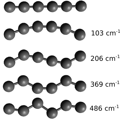
Figure 1: The relative amplitudes of the normal coordinates for the four doubly degenerate vibrational modes of C₆. The representations of the modes are chosen so all motion of the atoms is in one plane. The top geometry corresponds to the vibrational ground-state structure.

The calculated vibrational frequencies are listed in Table 1, together with the experimental values, given in [30]. While the lowest-energy modes are well reproduced by the calculations, some deviations are seen for the higher frequency modes. Overall, however, the calculated values are in fair agreement with the experimental values. Many of the modes have a dipole moment of zero, preventing detection by infrared spectroscopy. For this reason, the analysis here will use the calculated frequencies.

Table 1: Calculated vibrational quantum energies of C₄, C₆ and C₇ in cm^-1. The doubly degenerate bending modes are indicated in bold. The experimental values [30] are shown below the theoretical values calculated here.

n	$\hbar\omega$ (cm-1)
4	169 346 937 1589 2120
4 Exp.	160, 339, 1549, 2032
6	103 206 369 486 668 1225 1729 2028 2179
6 Exp.	90, 246, 637, 1197, 1694, 1960, 2061
7	77 168 264 527 585 676 1112 1600 1980 2212 2245
7 Exp.	496, 548, 1893, 2128

Fig.(2) shows the results of a calculation of the angular momentum specified level densities of C_4,6,7 with Eq.Level densities for a series of total excitation energies. The highest energies in the calculations were chosen to be on the order of magnitude of the excitation energies of clusters that decay on typical mass spectroscopic time scales of tens to hundreds of microseconds.

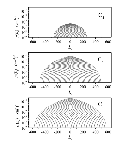
Figure 2: The angular momenta specified level density for different total excitation energies for the clusters indicated in the frames, all on identical scales. The curves are from top to bottom for $E=44000$ cm^-1 down to 2000 cm^-1 in steps of 2000 cm^-1 in all three cases. $L_{z}$ is given in units of $\hbar$.

A zoomed view of the values for C₆ around $L_{z}=0$ is shown in Fig.(3).

Figure 3: A zoomed view of Fig.(2) for C₆.

Microcanonical temperature, $L_{z}$-resolved

Although the values shown in Figs.(2,3) are microcanonical, it is nevertheless possible and occasionally also convenient to define a temperature for such systems. This temperature is particularly useful for the interpretation of measured kinetic energy release distributions (KERDs), because it allows these distributions to be written with what is effectively a Boltzmann factor multiplied by phase space factors etc. [31]. The definition is (with $k_{B}$ set to unity)

$$T^{-1}\equiv\left.\frac{\partial\rho(E,L_{z})}{\partial E}\right|_{L_{z}}.$$ (12)

Fig.(4) shows the microcanonical temperature for different angular momentum sectors of the level density.

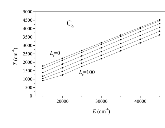
Figure 4: The microcanonical temperature for the angular momentum specified states. The values are calculated numerically with a finite derivative over 1000 cm^-1, centered at the abscissa values, with Eq.12. The curves show the values for $L_{z}=0\hbar$ to $100\hbar$, in steps of $20\hbar$ (top to bottom).

The slopes are clearly all very similar. They are also very close to the value of $n-1$ which is expected for $n$ harmonic oscillators (the -1 is the difference between canonical and microcanonical heat capacities, see [32] for details). The two other cluster sizes calculated give similar results. Although heat capacities are thus fairly insensitive to the precise value of the angular momentum, the temperature has a clear angular momentum dependence. The higher the angular momentum, the lower the temperature. In conjunction with the constant heat capacity, this suggests that the angular momentum comes with a price. Effectively, it ties up energy and reduces the available phase space for the other vibrations. For the C₆ clusters, the lowering of the microcanonical temperature corresponds to a shift in energy of about 250 cm^-1 for each time two units of $\hbar$ are added, in the high energy limit. This is reasonably close to the average frequency of 291 cm^-1 of the bending modes to assign this shift to the excitation required to reach the specified angular momentum.

As one application of the results derived, the effective Boltzmann factor that enters the kinetic energy release distributions will be calculated. A number of theories are available from the literature for the calculation of the rest of these distributions. A discussion of these theories will lead us too far astray and we will simply consider the Boltzmann factor here.

We will limit ourselves to consider the expression of a product arising from a reactant with zero initial vibrational angular momentum. The function to be approximated is then $\rho(E-\varepsilon,L_{z})$, where $E$ is the product energy before deduction of $\varepsilon$, the kinetic energy released, and $L_{z}$ is the resulting vibrational mode angular momentum. The logarithm of $\rho$ is expanded to first order in $\varepsilon$ to give

$$\rho(E-\varepsilon,L_{z})\approx\rho(E,L_{z})\exp\left(-\frac{\varepsilon}{T(E,L_{z})}\right).$$ (13)

The temperatures are given by the calculated values in Fig.(4) for C₆. The temperatures decrease approximately with 11 cm^-1 each time $L_{z}$ increases by one unit of $\hbar$. The approximation sign in Eq.13 refers to the fact that the rate of decrease with $L_{z}$ for low values (below $20\hbar$) is less. As the values taken by $L_{z}$ cover a wider range (see top line of Fig.(3), we will ignore this and represent the temperature for the case of C₆ as:

$$T(E,L_{z})=T(E,L_{z}=0)-11\frac{{\rm cm}^{-1}}{\hbar}L_{z}.$$ (14)

The coefficient of 11 cm^-1 is on the order of the price in energy per unit of angular momentum, which we saw above to be about 250/2 cm^-1, divided by the number of vibrational degrees of freedom, $3n-5=13$, or 10 cm^-1, in good agreement with the fitted value of 11 cm^-1. For the C₆ case we can therefore write Eq.13 as

$$\rho(E-\varepsilon,L_{z})\approx\rho(E,L_{z})\exp\left(-\frac{\varepsilon}{T(E,0)-11\frac{{\rm cm}^{-1}}{\hbar}L_{z}}\right).$$ (15)

The result in Eq.15 shows that the effective temperature as measured with KERDs for a given total excitation energy decreases with increasing angular momentum. The $L_{z}$ dependence at high excitation energies can be fitted with the function

$$\rho(E,L_{z})\approx\rho(E,0)\exp\left(-a|L_{z}|^{1.7}\right),$$ (16)

around the peak at $L_{z}=0$. The value of the coefficient is $a=6\times 10^{-4}$ for the highest energy curve shown in Fig.(3). This can then be used as is or expanded further with $L_{z}\rightarrow L_{z}+\delta L_{z}$.

The factor $\rho(E,L_{z})$ is part of the normalization of the KERD’s, and the entire distribution will then be determined by the two exponentials and the prefactor which will not be discussed in detail here. Disregarding this prefactor, the decay will be biased toward a reduction of the absolute value of the angular momentum.

The $L_{z}$ distributions will vary with the experimental conditions. To nevertheless give some information on the effect of the vibrational angular momentum, the effect will be illustrated with a schematic calculation. The KER distributions will be represented by the derived Boltzmann factor and the preexponential phase space factor combined with the kinematic speed factor [31]. These two factors combine to a factor of kinetic energy to the power one. For the product C₆ with the final state energy $E$, $L_{z}$ and fragment translational kinetic energy $\varepsilon$ this becomes:

$$P(E,L_{z},\epsilon){\rm d}\varepsilon propto\rho\left(E,L_{z}\right)\varepsilon\exp\left(-\frac{\varepsilon}{T(E,0)-11\frac{\rm cm^{-1}}{\hbar}L_{z}}\right){\rm d}\varepsilon,$$ (17)

where $L_{z}$ is the final state vibrational angular momentum. This is then the expression for zero initial $L_{z}$. The curves for $L_{z}=0,40~{}\hbar$, $E=20000$ cm^-1 are shown in Fig.(5).

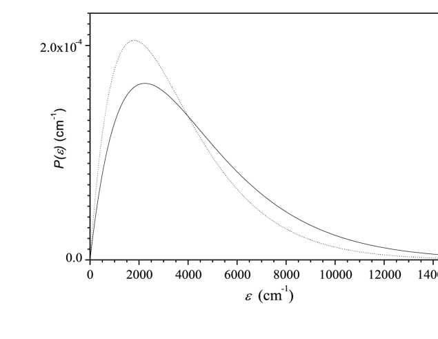
Figure 5: The schematic kinetic energy release distributions calculated for C₆ with final state energy $E$ and the two $L_{z}/\hbar$ values of 0 (full line) and 40 (dotted line). The energy is 20000 cm^-1. The microcanonical temperature is calculated to 2238 cm^-1 for this energy. The values of $\rho(E,0)$ and $\rho(E,40)$ differ by a factor of ca. 3 for this energy. The temperatures differ by 20 %. The curves are normalized to identical areas.

Canonical values

The canonical equilibrium values are likewise interesting. With the level structure found above, the canonical partition function is easily calculated and the angular momentum specified populations, $P(L_{z}=n\hbar)\equiv P(n)$ found for one degenerate pair of modes with frequency $\omega$ to be

$$P(0) = \left(1-{\rm e}^{-2\beta\hbar\omega}\right)^{-1}\frac{1}{Z},$$ (18)

$$P(\pm n,n>0) = {\rm e}^{-n\beta\hbar\omega}P(0),$$

where the total partition function is

$$Z=\left(1-{\rm e}^{-\beta\hbar\omega}\right)^{-2}.$$ (19)

The zero of the energy is set equal to the zero point energy of the oscillators here. The mean value of $L_{z}$ given by these distributions is obviously zero. The mean square is calculated to

$$\frac{1}{\hbar^{2}}\langle L_{z}^{2}\rangle = P(0)\sum_{n=-\infty}^{\infty}n^{2}{\rm e}^{-|n|\beta\hbar\omega}$$

$$= 2P(0)\left(\frac{1}{\hbar\omega}\right)^{2}\frac{\partial^{2}}{\partial\beta^{2}}\left(1-{\rm e}^{-\beta\hbar\omega}\right)^{-1}$$

$$= 2{\rm e}^{-\beta\hbar\omega}\frac{1+{\rm e}^{-\beta\hbar\omega}}{\left(1-{\rm e}^{-2\beta\hbar\omega}\right)\left(1-{\rm e}^{-\beta\hbar\omega}\right)}.$$

The square root of this function, $\langle L_{z}^{2}\rangle^{1/2}/\hbar$, shown in Fig.(6), is an almost straight line as a function of $T/\hbar\omega$, with a small offset close to zero.

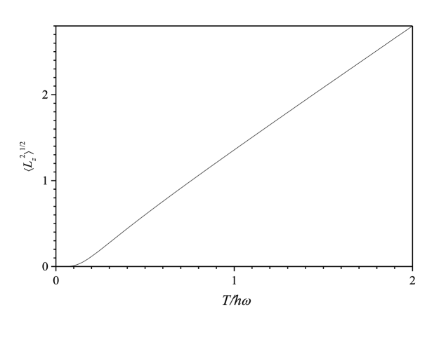
Figure 6: The root-mean-square of $L_{z}$ in units of $\hbar$ as a function of the reduced temperature for a single pair of degenerate oscillators.

Unity is reached at $T=0.76~{}\hbar\omega$. This means that the mode will contribute with angular momenta quanta even for temperatures below the value corresponding to the vibrational quantum energies. For the calculated lowest frequency of C₆ the value $T=0.76~{}\hbar\omega$ corresponds to a temperature of 112 K, and for the highest frequency to 531 K. Both of these are fairly modest temperatures for carbon chemistry.

Summary

Eq.Level densities is the main results of this work. The numerical prescription derived should be applicable to any linear molecule with known vibrational frequencies. If the total vibrational level density specified with respect to both energy and angular momentum is needed, this is calculated by a simple convolution of the level densities for the modes that carry angular momentum with those that do not.

1 Acknowledgements

PF acknowledges a Postdoctoral grant from the Research Foundation – Flanders (FWO).

References

- Atkins and Friedman [2011] P. Atkins and R. Friedman, Molecular Quantum Mechanics (Oxford University Press, Oxford, 2011).
- Lamb [1881] H. Lamb, Proc. London Math. Soc. s1-13, 189 (1881).
- Kuok et al. [2003] M. H. Kuok, H. S. Lim, S. C. Ng, N. N. Liu, and Z. K. Wang, Phys. Rev. Lett. 90, 255502 (2003).
- Hansen et al. [2007] K. Hansen, M. D. Johnson, and V. V. Kresin, Phys. Rev. B 76, 235424 (2007).
- Wilson [1935] E. B. Wilson, J. Chem. Phys. 3 (1935).
- Nielsen [1949] H. H. Nielsen, Phys. Rev. 75, 1961 (1949).
- Nielsen [1951] H. H. Nielsen, Rev. Mod. Phys. 23, 90 (1951).
- Oka [1967] T. Oka, J. Chem. Phys. 47, 5410 (1967).
- Watson [1968] J. K. G. Watson, Molecular Phys. 15, 479 (1968).
- Mills [1972] I. M. Mills, Vibration-Rotation Structure in Asymmetric and Symmetric-Top Molecules (Academic Press, 1972).
- Nemes [1984] L. Nemes, Acta Physica Hungarica 55, 97 (1984).
- Mielke et al. [2013] S. L. Mielke, A. Chakraborty, and D. G. Truhlar, J. Phys. Chem. A 117, 7327 (2013).
- Pan et al. [2016] H. Pan, Y. Cheng, and K. Liu, J. Phys. Chem. A 120, 4799 (2016).
- Esplin et al. [1989] M. P. Esplin, R. B. Wattson, M. L. Hoke, R. L. Hawkins, and L. S. Rothman, Appl Optics 28, 409 (1989).
- Alvarez-Estrada [1991] R. F. Alvarez-Estrada, Phys. Lett. A 159 (1991).
- Hirano et al. [2018] T. Hirano, U. Nagashima, and P. Jensen, J. Mol. Spec. 343, 54 (2018).
- Mordaunt et al. [1998] D. H. Mordaunt, M. N. R. Ashfold, R. N. Dixon, P. Löffler, L. Schnieder, and K. H. Welge, J. Chem. Phys. 108, 519 (1998).
- McLellan [1988] A. G. McLellan, J. Phys. C: Solid State Phys. 21, 1177 (1988).
- Zhang and Niu [2014] L. Zhang and Q. Niu, Phys. Rev. Lett. 112, 085503 (2014).
- McLellan [1989] A. G. McLellan, J. Mol. Spec. 134, 32 (1989).
- Liu et al. [2000] Y. F. Liu, W. J. Huo, and J. Y. Zeng, Comm. Theo. Phys. 33, 487 (2000).
- Liu et al. [1998] Y. F. Liu, W. J. Huo, and J. Y. Zeng, Phys. Rev. A 58, 862 (1998).
- Mota et al. [2002] R. D. Mota, V. D. Granados, A. Queijeiro, and J. Garćia, J. Phys. A: Math. Gen. 35, 2979 (2002).
- Beyer and Swinehart [1973] T. Beyer and D. F. Swinehart, Comm. Assoc. Comput. Machines 16, 379 (1973).
- Hansen [2008] K. Hansen, J. Chem. Phys. 128, 194103 (2008).
- Yen and Lai [2015] T. Yen and S. Lai, J. Chem. Phys. 142, 084313 (2015).
- Neese [2012] F. Neese, WIREs Computational Molecular Science 2, 73 (2012).
- Martínez and Alonso [2018] J. I. Martínez and J. A. Alonso, Phys. Chem. Chem. Phys. 20, 27368 (2018).
- van Orden and Saykally [1998] A. van Orden and R. J. Saykally, Chem. Rev. 98, 2313 (1998).
- Do and Besley [2015] H. Do and N. A. Besley, Phys. Chem. Chem. Phys. 17, 3898 (2015).
- Hansen [2018] K. Hansen, Statistical Physics of Nanoparticles in the Gas Phase, vol. 73 of Springer Series on Atomic, Optical, and Plasma Physics (Springer, Dordrecht, 2018).
- Andersen et al. [2001] J. U. Andersen, E. Bonderup, and K. Hansen, J. Chem. Phys. 114, 6518 (2001), URL https://doi.org/10.1063/1.1357794.