Approximation of Hysteresis Functional

Abstract

We develop a practical discrete model of hysteresis based on nonlinear play and generalized play, for use in first-order conservation laws with applications to adsorption-desorption hysteresis models. The model is easy to calibrate from sparse data, and offers rich secondary curves. We compare it with discrete regularized Preisach models. We also prove well-posedness and numerical stability of the class of hysteresis operators involving all those types, describe implementation and present numerical examples using experimental data.

1 Introduction

In this paper we describe and analyze a new robust and fairly simple algorithm for approximation and calibration of hysteresis functionals $u\to w=\mathcal{H}(u)$ which can be used in numerical schemes for PDEs arising in the applications. This paper extends the results in [39] to a broader class of hysteresis models. We explain how the model is calibrated, provide details on the solver, and compare the advantages and disadvantages of the different hysteresis constructions. Our work is motivated by the applications to flow and transport in porous media, and specifically by the adsorption–desorption hysteresis [13, 44, 21, 28, 33] which is significant and important in modeling of carbon sequestration [18, 11, 41, 37, 4, 56] and wood science and engineering [43, 12]. We consider the PDE model

$$\tfrac{\partial}{\partial t}(a(u)+\mathcal{H}(u))+A(u)=f,$$ (1)

in which $u$ is the unknown, $f$ is an external source, $A$ is a transport operator (advective and/or diffusive, generally nonlinear), and $a(\cdot)$ is a strongly monotone function. The problem is posed in the sense of distributions, in a functional space to be made precise below, and with some boundary and initial data.

Hysteresis is a well known nonlinear phenomenon in which the output of a process depends not only on the independent variable, but also on the history of the process, in a rate independent way. Hysteresis is well known to occur in electromagnetism [19, 14, 55], plasticity [34, 48, 3], phase transitions [29, 16, 47], multiphase flow in porous media [49, 40, 35, 23, 6, 45, 10], and many other applications [2, 17] including food processing and ecology [1, 31, 5]. The hysteresis models have been well studied, and the models range from simple to complex, with the latter requiring detailed data; see, e.g., the monographs and reviews in [24, 32, 55, 9, 30]. In particular, the ingenious well-known and well analyzed Preisach model considers a collection of (input, output) pairs from data $\mathcal{D}=(u(t),w(t))$ for $u\in\mathcal{D}_{u}=\{u:u(u,w)\in\mathcal{D}\}$, with $\mathcal{D}_{u}$ dense in $C([0,T])$, and records the hysteretic output $u\to w=\mathcal{H}(u)$ in the so-called Preisach plane. This record is then used to build $w=\mathcal{H}(u)$ as an integral over a continuum of parameters, for an arbitrary input $u$. See [52, 53, 14, 25, 15, 30].

However, experimental data $\mathcal{D}$ for hysteresis is frequently sparse rather than dense [18, 43, 41]; this limits the use of the Preisach model; in addition, its discrete form produces a very rough output $w(t)$. Our aim here is to approximate $\mathcal{H}(u)$ with a practical tunable hysteresis model producing a piecewise smooth $w(t)$ when $\mathcal{D}$ is only modest. An alternative is to ignore the hysteretic nature of $\mathcal{H}(u)$, but this may lead to substantial modeling errors in predictive simulations of (1) [4, 23].

The data in $\mathcal{D}$ includes, at the minimum, the boundary $H$ of the graph $(u,\mathcal{H}(u))$; see Fig. 2 for illustration. In particular, $H$ contains the “left” and “right” bounding curves $\gamma_{l}(u)$ and $\gamma_{r}(u)$ called primary scanning curves; here $\gamma_{r}(u)\leq\gamma_{l}(u)$ are piecewise smooth monotone increasing functions. When the input $u(t)$ is increasing, the output $w(t)\in\mathcal{H}(u(t))$ eventually reaches the curve $\gamma_{r}$, which it then follows upward. Similarly, when $u(t)$ decreases, the output $w(t)\in\mathcal{H}(u(t))$ eventually reaches and descends along the curve $\gamma_{l}$. When the input changes direction, $w(t)$ switches between $\gamma_{l}$ and $\gamma_{r}$ along the secondary scanning curves prescribed by the particular model. Since the models we consider are approximate, we usually obtain $H^{*}\approx H$ and $\mathcal{H}^{*}(u)\approx\mathcal{H}(u)$.

Example

Consider the adsorption of a chemical of concentration $u(t)$ in the fluid at a point within a porous medium, and let $w(t)$ be the concentration of that chemical that is adsorbed onto or desorbed from the particles of the porous medium. Classical models assume these are related by a function $w=b(u)$ of Langmuir type. However, $u$ and $w$ are related more generally by a hysteresis relationship: they follow one path when they increase and another when they decrease. For an explicit example we assume the amount of solute $w$ adsorbed by the porous medium increases according to $w=u$ up to a maximum adsorbed concentration of $4$, but it desorbs from there only after $u$ has decreased to $2$ and thereafter is given by $w=2u$. (See Figure 1, Left.) Such a relationship can be described with the truncation function $b(s)=s^{+}-(s-4)^{+}$: it increases along the right scanning curve $w=\gamma_{r}(u)=b(u)$ and decreases along the left scanning curve $w=\gamma_{l}(u)=b(2u)$. We assume further that $w=b(v)$ is constant between these curves, i.e., when $u<v<2u$. For example, if the fluid concentration $u(t)$ at a point increases from $0$ to $5$, the amount adsorbed onto the medium at that point is $w(t)=b(u(t))$. As the concentration decreases from $5$ down to $0$, the adsorbed amount decreases according to $w(t)=b(2u(t))$. The adsorbed concentration $w(u)=\mathcal{H}(u)$ and the total concentration $m(u)=u+w(u)$ are given by

$$w(u)=\begin{cases}u,\ &0\leq u\leq 4,\text{ increasing},\\ 4,\ &4<u\leq 5,\text{ increasing},\\ 4,\ &5>u\geq 2,\text{ decreasing},\\ 2u,\ &2>u\geq 0,\text{ decreasing},\end{cases}\qquad m(u)=\begin{cases}2u,\ &0\leq u\leq 4,\text{ increasing},\\ u+4,\ &4<u\leq 5,\text{ increasing},\\ u+4,\ &5>u\geq 2,\text{ decreasing},\\ 3u,\ &2>u\geq 0,\text{ decreasing}.\end{cases}$$ (2)

These relations are rate independent. Since the adsorbed amount depends not just on the current value of the fluid concentration but on its history, it is a hysteresis functional of the fluid concentration denoted by $w=\mathcal{H}(u)$. Note that the path (2) would be followed for instance by the solution of the initial-value problem

$$\begin{array}[]{cc}\tfrac{d}{dt}(u+\mathcal{H}(u))=f(t),\\ (u+\mathcal{H}(u))(0)=0,\end{array}\quad f(t)=\begin{cases}1,\ 0\leq t\leq 9,\\ -1,\ 9\leq t\leq 18.\end{cases}$$ (3)

The same path would be followed for any source function $f(t)$ which causes $u$ to increase monotonically from $0$ to $5$ and then to decrease monotonically from $5$ to $0$.

Suppose an adsorbing porous medium occupies the narrow tube $\{x:x\geq 0\}$, it is fully-saturated with fluid, and initially neither contains any solute. If fluid enters the medium at $x=0$ with a solute concentration of $\varphi(t)$ and it flows rightward with unit velocity, the solute concentration in the fluid $u(x,t)$ and the adsorbed solute concentration $w(x,t)$ satisfy the initial-boundary-value problem

$$\tfrac{\partial}{\partial t}(u+w)+\tfrac{\partial}{\partial x}u=0,\ w=\mathcal{H}(u),$$ (4a)

$$u(x,0)=w(x,0)=0,\ u(0,t)=\varphi(t),\ x>0,\ t>0.$$ (4b)

Let the boundary values of the incoming fluid concentration be given by $\varphi(t)=t,\ 0\leq t\leq 5,\textbf{ and }\varphi(t)=10-t,\ 5<t\leq 10.$ The fluid concentration $u(x,t)$ and the adsorbed concentration $w(x,t)$ within the medium satisfy this nonlinear transport equation and are given in the Figure 1 below at discrete times $t\in\{4,5,6,7,8,9\}$. The boundary-values are translated rightward with speed $1/2$ when $0\leq t\leq 4$. The characteristic speed jumps to $1$ at $x=0$ when $t=4$, and a shock develops then. (Note $u(x,5)$ and later.) A rarefraction wave is initiated at $x=0$ when $t=8$ and the characteristic speed drops to $1/3$. (Note $u(x,9)$.)

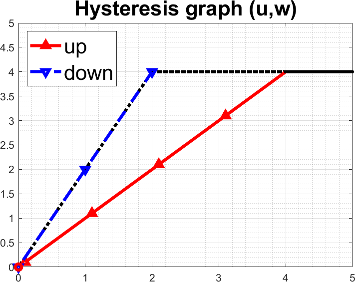
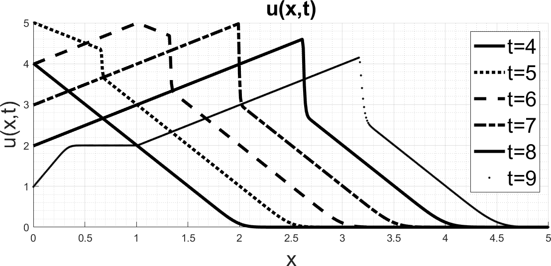
Figure 1: Adsorption hysteresis example. Left: graph $(u,w)$. Middle: plot of $u(x,t)$. Right: plot of $w(x,t)$ at selected times as shown.

$K$-generalized play family of models

The approach called $K$-generalized play is an umbrella for a family of flexible models $\mathcal{H}(\Pi^{K};u)$ calibrated from $H$ alone. Overall, the difficulty of approximating $H^{*}\approx H$ is not very different from that in the approximation of $\gamma_{l}(\cdot),\gamma_{r}(\cdot)$ by continuous piecewise linear or by step functions. The model $\mathcal{H}(\Pi^{K};u)$ has $K$ components with parameters encoded in an array $\Pi=\Pi^{K}\in\mathbb{R}^{K\times 4}$ calibrated from $H$. The model can be enriched if $\mathcal{D}$ includes data on internal loops. The class of $K$-generalized play models includes (i) generalized play as well as (ii) a discrete version $K$-Preisach of the Preisach model, as well as the most useful subclass called (iii) $K$-nonlinear play; these are known from the literature [24, 32, 55], but our calibration efforts and theory for discrete models for (1) is new. More generally, one can construct $\mathcal{H}(\Pi;\cdot)$ with some infinite dimensional $\Pi$ calibrated from a dense $\mathcal{D}$, e.g., $\Pi$ may represent the information in Preisach plane found from $\mathcal{D}$. We present a brief overview of (i-iii) now.

(i) The well-known generalized play model follows $\gamma_{l}(\cdot)$ and $\gamma_{r}(\cdot)$ exactly. It is given by an auxiliary evolution equation with time-dependent constraints

$$\tfrac{d}{dt}{v}(t)+\mathcal{C}(\gamma_{r}(u(t)),\gamma_{l}(u(t));v(t))\ni 0,\;\;v(0)=v^{init}\in\mathbb{R},$$ (5)

where $\mathcal{C}(a,b;r)$ is a constraint graph which enforces $a\leq r\leq b$; see details in Sec. 2. The output can be further transformed by $w=\mu b(v(t))$ with some monotone $b(\cdot)$, and $\mu>0$. In fact, one can consider a family of $K$ generalized play models, each expressed by $w_{k}=\mu_{k}b_{k}(v_{k})$ with $v_{k}$ given by (5) with primary curves $\gamma_{l,k},\gamma_{r,k}$. These are added together so $w=\sum_{k}w_{k}$; the parameters $\mu_{k},\gamma_{l,k},\gamma_{r,k},b_{k}$ are recorded in $k$’th row of $\Pi$. The generalized play model is conceptually simple and fairly easy to implement and is amenable to analyses. In addition, the output $\mathcal{H}(\Pi;u)$ exactly matches $H$ if $u$ is designed to sweep it. Its disadvantage is that the secondary scanning curves are only horizontal lines.

In (ii-iii), the $K$-Preisach and $K$-nonlinear play models have the same functional form $w=\mathcal{H}(\Pi^{K};u)=\sum_{k}\mu_{k}b_{k}(v_{k})$ where each $v_{k}$ solves an auxiliary linear play problem problem of the form (5) but with the constraint graphs $\gamma_{r}(u)=u-\beta_{k}$, $\gamma_{l}(u)=u-\alpha_{k}$, where $\alpha_{k}\leq\beta_{k}$. However, $K$-Preisach and $K$-nonlinear play  have different properties. (ii) The discrete version $K$-Preisach of the Preisach model is built with $K$ step functions approximating the curves $\gamma_{l}$ and $\gamma_{r}$ thus it feature discontinuities; therefore, regularization and extra effort by nonlinear solvers is required, while a rather rugged approximation $H^{*}$ of $H$ emerges even when $K=O(100)$. Its advantage is that it requires very little effort in calibration.

As a middle ground, we propose to calibrate the (iii) $K$-nonlinear play model which aims to adhere to the piecewise linear interpolants of $\gamma_{l}$ and $\gamma_{r}$. The model has some restrictions, and may require $K=O(100)$; we give details in Sec. 3. However, the quality of $H^{*}\approx H$ is high, while the model can be enhanced when $\mathcal{D}$ is more rich; we provide an outlook in Sec. 7.

Numerical analysis of $K$-generalized play

The analysis of numerical schemes for parabolic PDEs given by (1) with (primarily Preisach) hysteresis was considered in many works; e.g., [52, 53]. In turn, in [39] we developed rigorous numerical analysis for the $K$-nonlinear play model when $A$ in (1) represents nonlinear advection. In this paper we extend these results to the $K$-generalized play model while proving some subtle auxiliary results. When combined with the analysis in [39], these give $TV_{T}$ stability of an explicit upwind scheme combined with a nonlinear solver for nonlinear advection only; see Sec. 5 and 6. We also confirm experimentally convergence of the scheme in the $u$ variable, and stability in $w$. Throughout, we compare the advantages and disadvantages of the models (i-iii). We discuss the computational complexity of accounting for hysteresis with our models in Sec. 6.5.

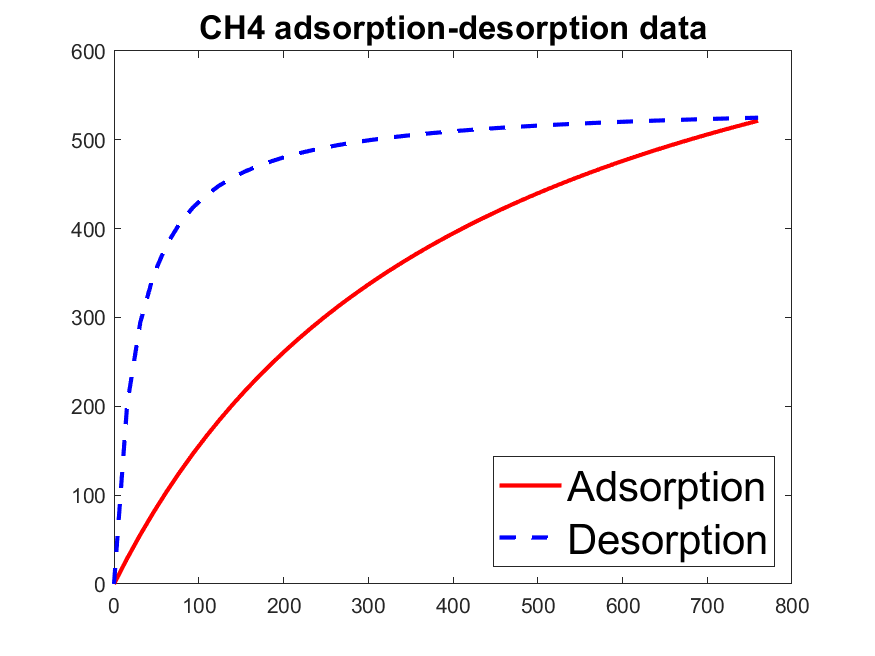
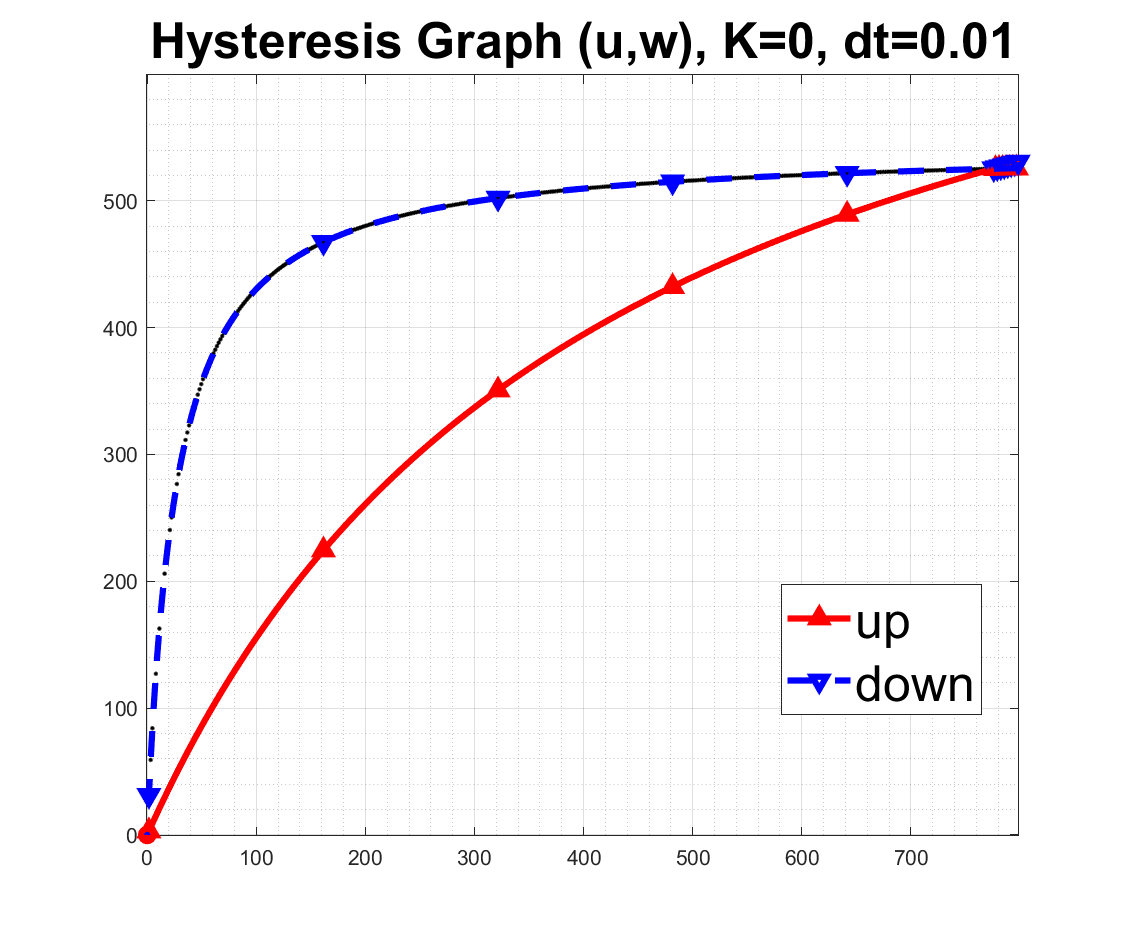
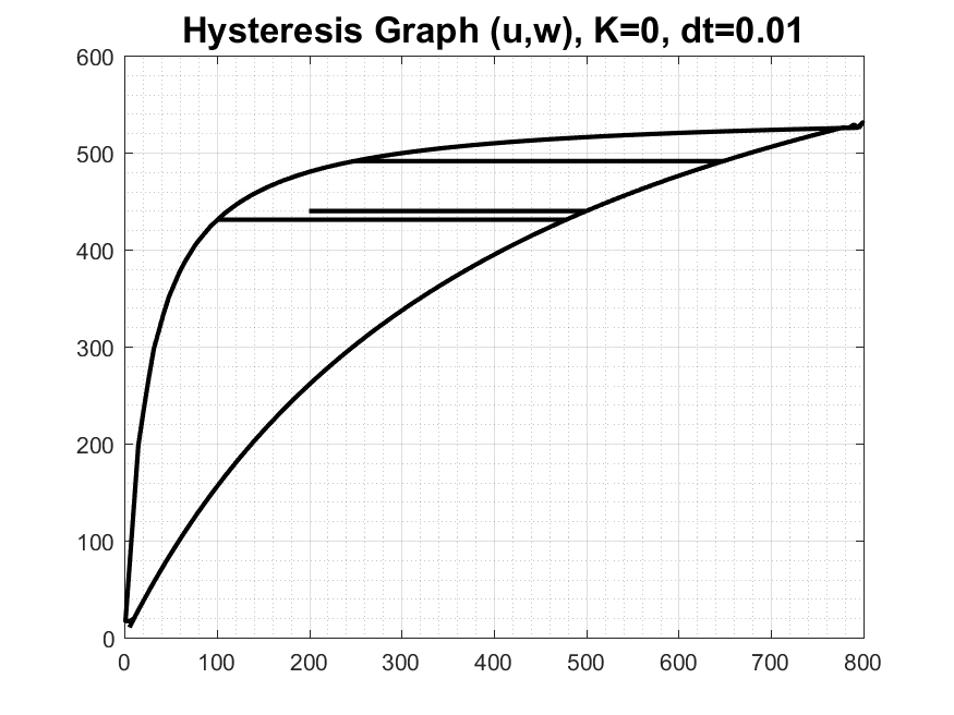
(a)	(b)	(c)

Figure 2: Modeling hysteresis given sparse data $\mathcal{D}$: (a) Experimental data $\mathcal{D}$ for $CH4$ adsorption–desorption hysteresis with only primary scanning curves $H$; (b) The output $\mathcal{H}(u)$ obtained with generalized play hysteresis model for a particular input $u(t)$ which sweeps $H$. (c) The output $\mathcal{H}(u)$with the same generalized play model for $u(t)$ which sweeps $H$ and includes a few secondary curves. Details for this example along with $K$-nonlinear play and $K$-Preisach graphs are in Sec. 4.6.4. $K=0$ denotes generalized play model.

Notation

Let $t$ denote time, and let $u(t)$ be an input function. We also allow $u=u(x,t)$ with $x\in\Omega$ where $\Omega\subset\mathbb{R}^{d}$ is some spatial domain; we drop $x$ when it is not relevant to the discussion. Consider the output $w(t)$ (or $w(x,t)$) obtained by some hysteresis model $w=\mathcal{H}(\Pi;u;v^{init})$ parametrized by a collection of parameters in $\Pi$. The output $w(t)$ also depends on the history through the auxiliary variable $v^{init}$. We drop $\Pi$ and $v^{init}$ when there is no need to single these out, and when this does not lead to confusion.

We distinguish between the operator $\mathcal{H}(\Pi;\cdot)$, and its graph $\mathcal{H}(\Pi)=(u,\mathcal{H}(\Pi;u))\subset\mathbb{R}^{2}$, when the inputs $u$ are from some family $\mathcal{D}_{u}$. At times, of interest is a fixed $u$ and the resulting trace $\mathcal{H}(\Pi;u)\subset\mathbb{R}^{2}$. We also denote the boundary of $\mathcal{H}(\Pi)$ by $H(\Pi)$. In particular most useful is the family $\mathcal{L}({\mathcal{U}})$ of continuous piecewise linear functions on $[0,T]$ identified by their peak values (local minima and maxima) given in the sequence ${\mathcal{U}}=[{\mathcal{U}}^{0},{\mathcal{U}}^{1},\ldots{\mathcal{U}}^{S}]$ corresponding to some (increasing) collection of time steps $\mathcal{T}=[T^{0},T^{1},\ldots T^{S}]$. Clearly $u\in\mathcal{L}({\mathcal{U}})$ is not differentiable at $t=T^{m}$. Note that the particular set $\mathcal{T}$ is unimportant since hysteresis is a rate-independent process.

Since only the derivative $\tfrac{\partial}{\partial t}{w}$ occurs in the PDE (1), a constant can be added to $w$ without change, so we can assume without loss of generality that the hysteresis output $\mathcal{H}(u)$ is non-negative.

We will consider the evolution on the time interval $(0,T]$ partitioned into discrete time steps $t_{n}=n\tau$ with uniform time step $\tau=T/N$. We will set $u(t_{n})=u^{n}$ and denote the approximations $U^{n}\approx u_{n}$, with similar notation for $w(\cdot)$ and other functions.

We will denote the identify function $x\to x$ with $\mathrm{id}$, and $x_{+}=\mathrm{max}(x,0)$.

Asssumptions

We proceed under the following conditions:

$$a(\cdot),b(\cdot),\gamma_{l}(\cdot),\gamma_{r}(\cdot)\text{ are {continuous monotone functions} on }\mathbb{R},$$ (6a)

$$a(\cdot)\text{ is strongly monotone, }b(\cdot)\text{ is Lipschitz continuous, and }$$ (6b)

$$\gamma_{r}(u)\leq\gamma_{l}(u)\text{ for }u\in\mathbb{R}.$$ (6c)

Without loss of generality, we assume that $a=\mathrm{id}+a_{0}$, where $a_{0}$ is continuous and non-decreasing on $\mathbb{R}$.

Plan of the paper

We discuss preliminaries in Sec. 2; we follow up in Sec. 3 with a discussion of $K$-generalized play hysteresis models including literature notes. In Sec. 4 we show how to calibrate $\Pi$ so that a given $H$ is the boundary of $\mathcal{H}(\Pi)$. In Sec. 5 we analyze the $K$-generalized play model. Section 6 contains a discussion of a solver, stability, convergence, and computational cost of an explicit–implicit numerical scheme for (1). In Sec. 7 we provide an outlook towards calibration of $\mathcal{H}(\cdot)$ with respect to secondary curves, and we summarize in Sec. 8. We also provide an Appendix with additional details.

2 ODE with constraint graphs and numerical approximation

In this section we provide the necessary definitions and references to relevant theory for (5) and its finite difference approximations. These are useful later in Sec. 5 for the study of (1), and for $\ell^{1}$ or $\ell^{2}$ estimates for ODE systems in $\mathbb{R}^{n}$.

2.1 ODE with maximal monotone graphs on a Hilbert space $V$

Consider a Hilbert space $V$, with inner product $(\cdot,\cdot)$, and norm $\mid\!\mid\!\cdot\!\mid\!\mid\!$. Let $\mathcal{C}(\cdot)$ be a multivalued operator, i.e., a relation on $V$: $\mathcal{C}\subseteq V\times V$. Its domain $\operatorname{Dom}(\mathcal{C})=\{v:[v,w]\in\mathcal{C}\}\subseteq V$ and range $\operatorname{Rg}(\mathcal{C})=\{w:[v,w]\in\mathcal{C}\}$ and inverse $\mathcal{C}^{-1}=\{[w,v]:[v,w]\in\mathcal{C}\}$ are defined as usual. We recall that $\mathcal{C}$ is monotone if $(v_{1}-v_{2},w_{1}-w_{2})_{V}\geq 0$ for any $v_{j},w_{j}\in V$ such that $w_{j}\in\mathcal{C}(v_{j})$; $\mathcal{C}$ is maximal monotone if also $\operatorname{Rg}(\mathcal{C}+I)=V$, and then it follows that $\operatorname{Rg}(\lambda\mathcal{C}+I)=V$ for all $\lambda>0$. Here $I$ is the identity operator. If $\mathcal{C}$ is maximal monotone and $\lambda>0$, the resolvent $R_{\mathcal{C}}^{\lambda}(\cdot)=(I+\lambda\mathcal{C})^{-1}(\cdot)$ is Lipschitz continuous on all of $V$, and the Yosida approximation of $\mathcal{C}$ is the function $\mathcal{C}^{\lambda}\equiv\frac{1}{\lambda}(I-R^{\lambda}_{\mathcal{C}})$. With $\tau>0$, the range of $(I+\tau\mathcal{C})$ is $V$, and the stationary problem,

$$v+\tau\mathcal{C}(v)\ni f\in V$$ (7)

has a unique solution given by $v=R_{\mathcal{C}}^{\tau}(f)$. The symbol $\ni$ is used in (7) because $\mathcal{C}(v)$ is, in general, a set. Once $v$ is found, the particular selection $c^{*}\in\mathcal{C}(v)$ is unique and equals $\tfrac{1}{\tau}(f-v)$.

2.1.1 Abstract Cauchy problem with a maximal monotone $\mathcal{C}$ on $V$

Let data $f\in L^{1}(0,T;V)$ and $v^{init}\in\overline{\operatorname{Dom}(\mathcal{C})}$,

$$\tfrac{d}{dt}v(t)+\mathcal{C}(v(t))\ni f(t),\ t\in(0,T],\ v(0)=v^{init}.$$ (8)

We choose approximations $F^{n}\approx f(t_{n})$ and approximate $v(t_{n})$ by successive finite difference solutions $V^{n}$ to

$$\frac{V^{n}-V^{n-1}}{\tau}+\mathcal{C}(V^{n})\ni F^{n},\quad 1\leq n\leq N,\ V^{0}=v^{init}.$$ (9)

These solutions $V^{n}$ are uniquely determined since they are given by the resolvent (7),

$$V^{n}=R_{\mathcal{C}}^{\tau}(V^{n-1}+\tau F^{n}).$$ (10)

The selection $c^{n}\in\mathcal{C}(V^{n})$ is unique at each $t_{n}$, with $\tau c^{n}=V^{n-1}+\tau F^{n}-V^{n}$.

The Cauchy problem (8) is well-posed and has a unique solution $v(\cdot)\in C([0,T];V)$ obtained as a limit of step-functions $v_{\tau}(t)$ built from $V^{n}$; see Sec. 5.2. Additionally, if $f\in W^{1,1}(0,T;V)$ and $v^{init}\in{\operatorname{Dom}(\mathcal{C})}$, then $v\in W^{1,\infty}(0,T;V)$ with $v(t)\in\operatorname{Dom}(\mathcal{C}),\ t\in[0,T]$. If $\mathcal{C}$ is a subgradient, $f\in L^{2}(0,T;V)$ and $v^{init}\in\overline{\operatorname{Dom}(\mathcal{C})}$, then $v\in W^{1,\infty}(\varepsilon,T;V)$ for $\varepsilon>0$ with $v(t)\in\operatorname{Dom}(\mathcal{C}),\ t\in(0,T]$. See [8, 46].

The meaning of inclusion $\ni$ in the ODE (8) is as follows. Rewritten as $\tfrac{dv}{dt}\in f-\mathcal{C}(v)$, the inclusion is replaced by an equality when $f-\mathcal{C}(v)$ is replaced by $(f(t+)-\mathcal{C}(v(t)))^{0}$, the element of $f-\mathcal{C}(v)$ of minimal norm; see [8] (pp. 66, 28).

2.1.2 Convergence of (9)

The proof of well-posedness discussed above relies on convergence of the step functions $v_{\tau}\to v$ as well as that of the piecewise linear interpolator $V_{\tau}$ of $V^{0},V^{1},\ldots,V^{N}$. We note that the solutions $v(t)$ need not be smooth, even if the input $u(t)$ is smooth. Generally $O(\tau)$ is the best rate in Hilbert space, otherwise the rate is $O(\sqrt{\tau})$. In the more general context of Banach space the rate depends on data $f$, e.g., whether $f\in H^{1}(0,T;V)$, and whether $v^{init}\in\operatorname{Dom}(\mathcal{C})$, and whether $\mathcal{C}$ is a subgradient. See [42] (Example 3); see also [36, 34], [48] (1.4, p41) for a-priori and a-posteriori analyses, also in application contexts such as in plasticity.

2.2 ODE with a fixed constraint graph on $\mathbb{R}$

Now we set $V=\mathbb{R}$, let $a\leq b$, and consider the non-empty closed interval $[a,b]\subset\mathbb{R}$. If $a<b$ we define

$$\mathcal{C}(a,b;s)=\begin{cases}(-\infty,0]\text{ if }s=a,\\ \{0\}\text{ if }a<s<b,\\ [0,\infty)\text{ if }s=b,\end{cases}\;\;R(a,b;s)=\begin{cases}a\text{ if }s\leq a,\\ s\text{ if }a<s<b,\\ b\text{ if }s\geq b,\end{cases}\;s\in\mathbb{R}.$$ (11)

This definition indicates that $\mathcal{C}(a,b;\cdot)$ is set-valued; its graph will be denoted by $\mathcal{C}(a,b)=\{a\}\times(-\infty,0]\cup(a,b)\times\{0\}\cup\{b\}\times[0,\infty]$, a maximal monotone relation on $\mathbb{R}\times\mathbb{R}$ with domain $\operatorname{Dom}{(\mathcal{C}(a,b))}=[a,b]$. We recall $\mathcal{C}(a,b;\cdot)=\partial I_{[a,b]}(\cdot)$ in $\mathbb{R}\times\mathbb{R}$ is the subgradient of the indicator function $I_{[a,b]}$ for the interval $[a,b]$: $I_{[a,b]}(x)=0$ if $x\in[a,b]$, and $=+\infty$ otherwise. It is clear that for any $\tau>0$ and any $s$ we have the equality of sets $\mathcal{C}(a,b;s)=\tau\mathcal{C}(a,b;s)$, so the resolvent $R(a,b;\cdot)=(I+\tau\mathcal{C}(a,b;\cdot))^{-1}=(I+\mathcal{C}(a,b;\cdot))^{-1}$ is independent of $\tau>0$; it can be written as $R(a,b;s)=\mathrm{min}\{\mathrm{max}\{a,s\},b\}$. The function $R(a,b;\cdot)$ is a monotone piecewise linear continuous function defined on $\mathbb{R}$ with range $[a,b]$, differentiable except at $\{a,b\}$; it is also Lipschitz continuous with a unit Lipschitz constant. When $a=b\in\mathbb{R}$, $\mathcal{C}(a,b;s)=(-\infty,\infty)$ if $s=a=b$, $\operatorname{Dom}{\mathcal{C}(a,b;\cdot)}=\left\{a\right\}$ is a single point, and the graph $\mathcal{C}(a,b;s)$ enforces $R(a,b;s)=a=b$ for any $s$.

With $\mathcal{C}(\cdot)=\mathcal{C}(a,b;\cdot)$, we obtain the finite difference solution to (8) using (10) and the resolvent $R_{\mathcal{C}}^{\tau}(\cdot)=R(a,b;\cdot)$. Alternatively, one can replace $\mathcal{C}(a,b;\cdot)$ in (8) by a smoother “penalty functional” which enforces $v(t)\in\operatorname{Dom}(\mathcal{C}(a,b;))=[a,b]$. Another possibility is to use a Lagrange multiplier, but elimination of Lagrange multiplier typically gives exactly (10).

2.3 ODE with a time-dependent constraint

In generalized play models of hysteresis (5) the constraints in $\mathcal{C}(a,b;\cdot)$ are time dependent and in fact depend on the input function $u(t)$, namely, $a(t)=\gamma_{r}(u(t))$, $b(t)=\gamma_{l}(u(t))$. Here $\gamma_{r},\gamma_{l}$ are continuous monotone functions, and $u(\cdot)\in C([0,T])$. We consider the IVP for (5)

$$\tfrac{d}{dt}v(t)+\mathcal{C}(\gamma_{r}(u(t)),\gamma_{l}(u(t));v(t))\ni 0,\ t\in(0,T],\ v(0)=v^{init}.$$ (12)

The approximation of (12) requires that we know $U^{1},U^{2},\ldots$ and then solve successively for $n\geq 1$

$$\frac{1}{\tau}(V^{n}-V^{n-1})+\mathcal{C}(\gamma_{r}(U^{n}),\gamma_{l}(U^{n});V^{n})\ni 0\,,\quad V^{0}=v^{init}\,.$$ (13)

Given $U^{n}$, and a fixed pair $\gamma_{l},\gamma_{r}$, we can write out the solution $V^{n}$ of this stationary problem, adapting (11) to define $\mathcal{R}_{\gamma}(\overline{V};\cdot)$ with $\overline{V}=V^{n-1}$

$$V^{n}=\mathcal{R}_{\gamma}(\overline{V};U^{n})\equiv R(\gamma_{r}(U^{n}),\gamma_{l}(U^{n});\;\overline{V})=\begin{cases}\gamma_{r}(U^{n})\text{ if }\overline{V}\leq\gamma_{r}(U^{n}),\\ \overline{V}\text{ if }\gamma_{r}(U^{n})<\overline{V}<\gamma_{l}(U^{n}),\\ \gamma_{l}(U^{n})\text{ if }\overline{V}\geq\gamma_{l}(U^{n}).\end{cases}$$ (14)

Various properties of (12)–(14) are needed in Sec. 5 and 6 when (12) is coupled with an evolution problem for $u(t)$. In particular, each $\mathcal{R}_{\gamma}(\overline{V};u)$ is differentiable at the points of differentiability of $\gamma_{l}(\cdot)$ and $\gamma_{r}(\cdot)$ except at $u=\gamma_{l}^{-1}(\overline{V})$ and at $u=\gamma_{r}^{-1}(\overline{V})$. In addition, we have the following monotonicity result

Lemma 1.

Assume $V^{n-1}\in\operatorname{Dom}(\mathcal{C}(\gamma_{r}(U^{n-1}),\gamma_{l}(U^{n-1});\cdot)$. Then

$$U^{n}\geq U^{n-1}\implies V^{n}={\mathcal{G}}(V^{n-1};U^{n})\geq V^{n-1},$$ (15)

$$U^{n}\leq U^{n-1}\implies V^{n}={\mathcal{G}}(V^{n-1};U^{n})\leq V^{n-1}.$$

Proof.

This property might or not be obvious, and is easiest to prove when $\gamma_{l}$ and $\gamma_{r}$ are injective. From the assumption $V^{n-1}\in\operatorname{Dom}(\mathcal{C}(\gamma_{r}(U^{n-1}),\gamma_{l}(U^{n-1});\cdot))$ which means $\gamma_{l}^{-1}(V^{n-1})\leq U^{n-1}\leq\gamma_{r}^{-1}(V^{n-1})$. Now the point $(U^{n},V^{n})$ with $V^{n}={\mathcal{G}}(V^{n-1};U^{n})$ is on the the graph of the monotone nondecreasing function (14) determined by $\gamma_{l}(\cdot)$ on the left, $\gamma_{r}(\cdot)$ on the right, with a “flat” connector at $v=V^{n-1}$. Thus $V^{n}\geq V^{n-1}$ whenever $U^{n}\geq U^{n-1}$ (the second part follows analogously). In the non-injective case we replace $\gamma_{l}^{-1}(V^{n-1})$, $\gamma_{r}^{-1}(V^{n-1})$ by $\min(\gamma_{l}^{-1}(V^{n-1}))$ and $\max(\gamma_{r}^{-1}(V^{n-1}))$, respectively. ∎

The special case of (12) with $\gamma_{r}(u)=u-\beta$, $\gamma_{l}(u)=u-\alpha$ for some $\alpha\leq\beta$ gives

$$\tfrac{d}{dt}v(t)+\mathcal{C}(u(t)-\beta,u(t)-\alpha;v(t))\ni 0,\ t\in(0,T],\ v(0)=v^{init},$$ (16)

with the approximation $\frac{1}{\tau}(V^{n}-V^{n-1})+\mathcal{C}(U^{n}-\beta,U^{n}-\alpha;V^{n})\ni 0\,,\quad V^{0}=v^{init}$. The counterpart of (14) with $\overline{V}=V^{n-1}$ can be written in two equivalent ways,

$$V^{n}=U^{n}+R(-\beta,-\alpha;\;\overline{V}-U^{n})=R(U^{n}-\beta,U^{n}-\alpha;\;\overline{V}).$$ (17)

2.4 Auxiliary implicit ODE: from v to $w=b(v)$

We recall now the following subtle relationship.

Lemma 2.

Assume $u\in C([0,T])$ and that $v\in W^{1,1}(0,T)$ is a strong solution of (12). Then $b(v(t))$ is the unique solution determined by $b(v(0))$ of

$$\tfrac{d}{dt}{b(v(t))}+\mathcal{C}(\gamma_{r}(u(t)),\gamma_{l}(u(t));v(t)) \ni 0.$$ (18)

Proof.

Let $v\in W^{1,1}(0,T)$ be a strong solution of (12). Since $b(\cdot)$ is Lipschitz, $w(t)\equiv b(v(t))$ is differentiable a.e., and the chain rule gives (by [22] (Cor. A.6))

$$w^{\prime}(t)=b^{\prime}(v(t))v^{\prime}(t)\in-b^{\prime}(v(t))\,\mathcal{C}(\gamma_{r}(u),\gamma_{l}(u);v(t))\subset-\mathcal{C}(\gamma_{r}(u),\gamma_{l}(u);v(t)),$$

where the last relation follows from $b^{\prime}(\cdot)\geq 0$.

If $v_{j}$ are strong solutions for $j=1,2$, set $w_{j}(t)=b(v_{j}(t))$, so $w_{j}^{\prime}(t)+\mathcal{C}(\gamma_{r}(u(t)),\gamma_{l}(u(t));v_{j}(t))\ni 0.$ From Theorem A.1 of [22], the absolutely continuous function $|w_{1}(t)-w_{2}(t)|$ is a.e. differentiable and satisfies

$$\tfrac{d}{dt}|w_{1}(t)-w_{2}(t)|=\operatorname{sgn}_{0}(w_{1}(t)-w_{2}(t))(w_{1}^{\prime}(t)-w_{2}^{\prime}(t))$$

$$\in-\operatorname{sgn}_{0}(w_{1}(t)-w_{2}(t))\big{(}\mathcal{C}(\gamma_{r}(u),\gamma_{l}(u);v_{1}(t))-\mathcal{C}(\gamma_{r}(u),\gamma_{l}(u);v_{2}(t))\big{)}.$$

If $w_{1}(t)-w_{2}(t)\neq 0$, then the last term is non-positive for any choices from the constraint relations, and so $|w_{1}(t)-w_{2}(t)|\leq|w_{1}(0)-w(0)|$ for $t\geq 0$. ∎

We also consider a discrete analogue of Lemma 2 for (18), and apply Lemma 1.

Lemma 3.

If (13) holds, then $W^{n}=b(V^{n})$ is the unique solution of

$$\frac{1}{\tau}(b(V^{n})-b(V^{n-1}))+\mathcal{C}(\gamma_{r}(U^{n}),\gamma_{l}(U^{n});V^{n})\ni 0\,,\quad b(V^{0})=b(v^{init})\,.$$ (19)

In addition, $U^{n}\geq U^{n-1}$ implies $W^{n}\geq W^{n-1}$.

3 Hysteresis models: generalized play, $K$-nonlinear play, $K$-Preisach, and related

Mathematical models of hysteresis have a long history, and much work has been devoted to their development and analysis. We refer to the monographs [54, 55, 32, 24] and the review paper [30] for overview and the detailed history of a large variety of hysteresis models.

	Linear	Nonlinear	Preisach	Generalized
$\mathcal{C}$	$\mathcal{C}(u-\beta,u-\alpha;v)$			$\mathcal{C}(\gamma_{r}(u),\gamma_{l}(u);v)$
$u\to v$	$u-\beta\leq v\leq u-\alpha$			$\gamma_{r}(u)\leq v\leq\gamma_{l}(u)$
	$\alpha\leq u-v\leq\beta$			$\gamma_{l}^{-1}(v)\leq u\leq\gamma_{r}^{-1}(v)$
truncation $b(v)$	id	$b^{h}_{h}$	$b^{h}_{0}$, $b^{h}_{\varepsilon}$ or $b^{h}_{*}$	id
primary	$v=u-\beta$ or $v=u-\alpha$	translate of $b(\cdot)$		$\gamma_{l}(u)$ or $\gamma_{r}(u)$
secondary	horizontal	horizontal		horizontal
parameters in $\Pi$	$\mu,\alpha,\beta,\infty$	$\mu,\alpha,\beta,h$	$\mu,\alpha,\beta,b^{h}_{s}$	$1,\gamma_{l}(\cdot)$, $\gamma_{r}(\cdot),\mathrm{id}$
reference	[38]	III.2, p64		III.2, p65

Table 1: Hysteresis (hysteron) operator choices. The input is $u(t)$. The output $v(t)$ satisfies $\gamma_{r}(u)\leq v\leq\gamma_{l}(u)$, and is scaled and truncated as in $\mathcal{H}(\Pi;u;v^{init})\ni w(t)=\mu b(v(t))$. For nonlinear play, we have $b(\cdot)=b^{h}(\cdot)$ and we record its parameter $h$. For Preisach hysteresis, $(s)=$0, or $\varepsilon$, or $*$, which indicates $b(\cdot)=b^{h}_{0},b^{h}_{\varepsilon},b^{h}_{*}$, respectively. For generalized play in principle we can have any $\mu$ and $b(\cdot)$, but these can be subsumed in the definition of $\gamma_{l},\gamma_{r}$, thus for simplicity we set $\mu=1$ and $b(\cdot)=\mathrm{id}$.

In this paper we focus on three types of play hysteresis models under a common umbrella of $K$-generalized play: generalized play, $K$-nonlinear play, and regularized $K$-Preisach, which we analyze, compare, and parametrize. The three types are interconnected. Generalized play can be approximated by $K$-nonlinear play. Furthermore, equivalent representation of Preisach model can be obtained as a superposition of an infinite number of unit hysterons of type nonlinear play; see [32] (p.31 and Fig. 1.32). These models are constructed with three steps which give output $w$ to input $u$ by adding $K$ unit hysterons $w_{k}$. Examples are given in Sec. 3.3.

(A) Play models.

We build unit hysterons with initial value problems (IVP) for either generalized play (12) or its special case, linear play (16), with some given $\alpha\leq\beta$, and primary curves $\gamma_{r}(u)=u-\beta,\gamma_{l}(u)=u-\alpha$. These models give output $v(t)$ which increases on $v(t)=\gamma_{r}(u(t))$, decreases on $v(t)=\gamma_{l}(u(t))$, and is constant between these bounding curves where it satisfies $\gamma_{r}(u(t))<v(t)<\gamma_{l}(u(t))$. We consider $K$ such auxiliary functions $v_{k}(u)$, each corresponding to its own $\gamma_{l,k},\gamma_{r,k}$.

(B) Truncation of play models.

The second step is to truncate each hysteron to limit the influence of the constraint. The output of the truncation is $b(v)$ as in Sec. 2.4, and is $b_{k}(v_{k}(u))$ for each $v_{k}$, where each $b_{k}(\cdot)$ is some arbitrary monotone nondecreasing function, possibly different for each $k$. Models $u\to b_{k}(v_{k}(u))$ are called nonlinear play [55]. The shape of each $b_{k}(v_{k}(u))$ follows the translates of $b(\cdot)$ (or $b_{k}$).

In particular we choose $b(\cdot)$ to be either $b^{\infty}=\mathrm{id}$ for the linear play, or a truncation function with bounded range $[0,h]$ for nonlinear play. Let $\varepsilon>0,h>0$ and define the scaled ramp function $b^{h}_{\varepsilon}(x)=\tfrac{h}{\varepsilon}(x_{+}-(x-\varepsilon)_{+})$, which has range $[0,h]$, slope $\tfrac{h}{\varepsilon}$ on $(0,\varepsilon)$, and equals $0$ for $x<0$ and $h$ for $x>\varepsilon$. The ramp function $b^{h}(x)=x_{+}-(x-h)_{+}$ is a particular case, with maximum slope $1$, and is the main building block in $K$-nonlinear play models, with unit hysterons of shape of truncated parallelograms.

The scaled left continuous Heaviside function $b^{h}_{0}$ equal to $b^{h}_{0}(x)=h$ when $x>0$ and $b^{h}_{0}(x)=0$ when $x\leq 0$ has “maximum slope” equal to $\infty$, and produces discontinuous outputs. The output $(u,w)$ forms a hysteron “box” of height $\mu h$ which is a building block of the discontinuous Preisach model, also called basic relay model [55] (p.97). These can be approximated by their Yosida approximations $b^{h}_{\varepsilon}(\cdot)$ as $\varepsilon\to 0$; we note $b^{h}=b^{h}_{\varepsilon}$ when $\varepsilon=1$. Also, $b^{h}_{0}$ can be approximated by some $C^{\infty}$ smooth function $b^{h}_{*}(v)$ with range $[0,h]$; here we use the appropriately scaled erf function

$$b^{h}_{*}(s)=h/2(\mathrm{erf}(2s-1)+1/2)),$$ (20)

but other choices are possible.

The steps (A-B) produce unit hysterons shown in Fig. 3. Note that a unit hysteron with $b^{h}_{0}$ has vertical sides and (6b) does not hold, thus $K$-Preisach model without regularization is not one of $K$-generalized play models. However, we include it in some illustrative examples.

(C) Linear combinations of unit hysterons.

Definition 1.

The $K$-generalized play model is determined by a family of constraint curves $\{\gamma_{r,k},\gamma_{l,k}\}$ and functions $b_{k}$, and scaling factors $\mu_{k}>0$. The output is

$$w(t)=\mathcal{H}(\Pi;u(t);v^{init}) = \sum_{k=1}^{K}w_{k}=\sum_{k=1}^{K}\mu_{k}b_{k}(v_{k}(u(t))),$$ (21a)

$$\tfrac{d}{dt}v_{k}(t)+\mathcal{C}(\gamma_{r,k}(u),\gamma_{l,k}(u);v_{k}(t)) \ni 0,\$$ (21b)

$$\quad v_{k}(0) = v^{init}_{k}\in[\gamma_{r,k}(u^{init}),\gamma_{l,k}(u^{init})],\quad 1\leq k\leq K.$$

We collect the parameters in a K-tuple $\Pi^{K}=(\Pi_{k})_{k=1}^{K}$. We also assume for the relevant data that

$$\gamma_{l,k},\gamma_{r,k},b_{k}\mathrm{\ satisfy\eqref{assumption-a},\eqref{assumption-b},\eqref{eq:assumlr}},$$ (22a)

$$b_{k}\mathrm{\ are\ one\ of\ those\ listed\ in\ (B)},$$ (22b)

$$\alpha_{k}\leq\beta_{k};h_{k}>0,\mu_{k}>0.$$ (22c)

Each row $\Pi_{k}$ of $\Pi$ represents a unit hysteron identified by either some functions or numbers or special symbols, with interpretation clear from the context, as in an object-oriented software environment. For example, the numbers are interpreted as parameters of some fixed functions, and the symbol $\infty$ or $\ast$ have a special meaning. Table 1 summarizes the notation for unit hysterons, and Table 2 the properties and notation for the family of $K$-generalized play. For simplicity we consider only hysteresis operators made of unit hysterons of the same type, even though our theoretical results as well as algorithms apply to the more general case.

We have the special cases of $[\mu_{k},\gamma_{l,k}(\cdot),\gamma_{r,k}(\cdot),b_{k}(\cdot)]$ denoted by

$$\Pi^{\gamma}\ni\Pi;\;\;\Pi_{k} = [1,\gamma_{l,k}(\cdot),\gamma_{r,k}(\cdot),\mathrm{id}],\;\;\mathrm{or}$$ (23a)

$$\Pi^{K,1}\ni\Pi;\;\;\Pi_{k} = [\mu_{k},\alpha_{k},\beta_{k},h_{k}],\;\;\mathrm{or}$$ (23b)

$$\Pi^{K}_{\infty}\ni\Pi;\;\;\Pi_{k} = [\mu_{k},\alpha_{k},\beta_{k},\infty],\;\;\mathrm{or}$$ (23c)

$$\Pi^{K,0}\cup\Pi^{K,\varepsilon}\cup\Pi^{K,*}\ni\Pi;\;\;\Pi_{k} = [\mu_{k},\alpha_{k},\beta_{k},b^{h_{k}}_{s_{k}}(\cdot)].$$ (23d)

The notation in (23) is similar to MATLAB matrix notation.

Additional remarks on (23) are as follows. In (23a), from a modeling point of view, it makes sense in for generalized play to subsume $\mu$ and $b^{h}$ in the definitions of $\gamma_{l},\gamma_{r}$, since the alternative leads to cumbersome calibration. In addition, in practice generalized play model uses only one component, but the keyword $K$-generalized play is useful to denote the entire umbrella of models when discussing theory and implementation. For Preisach model in (23d), the maximum slope $s$ of $b^{h_{k}}_{r_{k}}(v)$ is the maximum of $1/r_{k}$, and is the superscript in the parameter array $\Pi^{K,\varepsilon}$, e.g., we have $s=\tfrac{1}{\epsilon}$ for $b^{h}_{\varepsilon}$. For the smooth choice $b_{k}=b^{h_{k}}_{*}$ we denote the variable slope by $*$ in $\Pi^{K,*}$. Also, $r=0$ for $b^{h}_{0}$ with “infinite” slope $s=\infty$, thus $b^{h}_{0}$ is not Lipschitz and not part of $K$-generalized play family. Finally, the special notation with symbols $\infty$ or $*$ need not to be interpreted literally in the formula (21a).

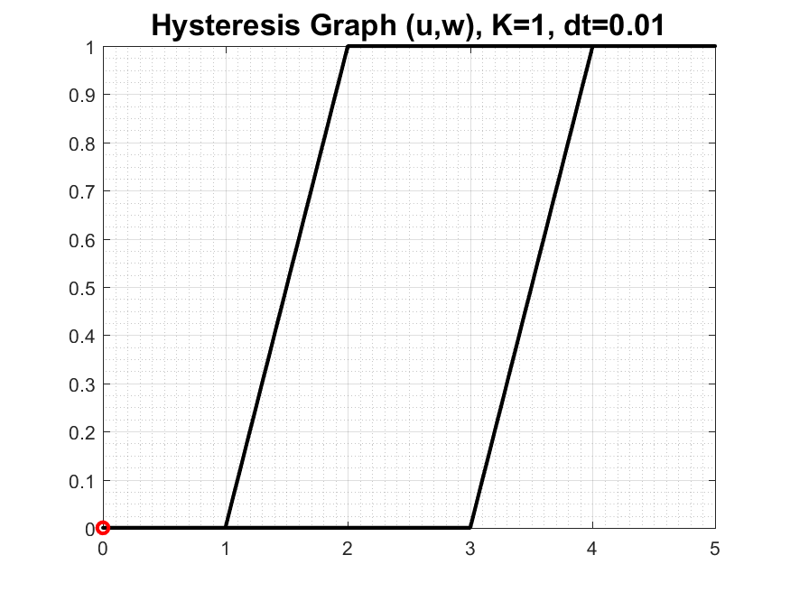
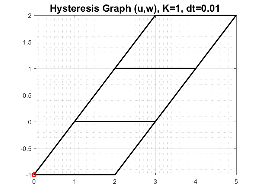
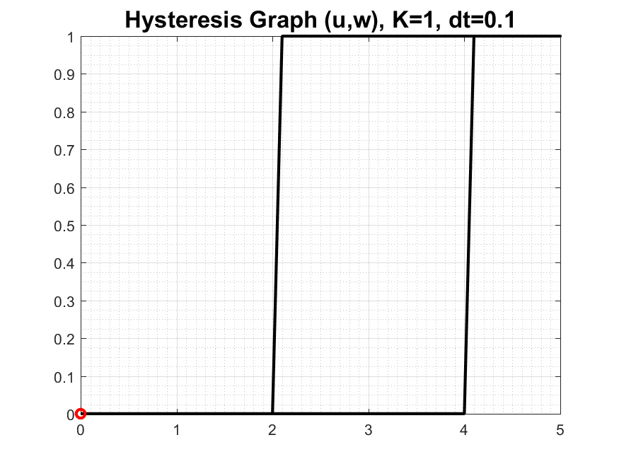
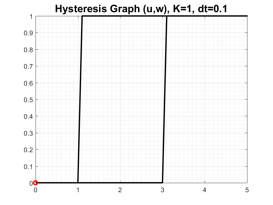
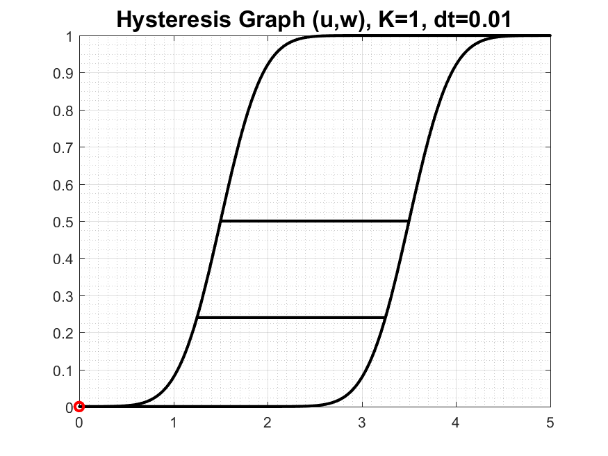
$\Pi^{1,1}$=$[1,1,3,1]$	$\Pi^{1}_{\infty}$=$[1,1,3,\infty]$	$\Pi^{1,0}$=$[1,1,3,b^{1}_{0}]$	$\Pi^{1,\varepsilon}$=$[100,1,3,1/100]$	$\Pi^{1,*}$=$[1,1,3,*]$
(i)	(ii)	(iii)	(iv)	(v)
nonlinear	linear	Preisach	(iv-v) regularized Preisach

Figure 3: Examples of unit hysterons from Sec. 3 with $\gamma_{r}(u)=u-3$ and $\gamma_{l}(u)=u-1$. Plotted are $H=\mathcal{H}(\Pi;u)$ with $\Pi$ as indicated and $u=\mathcal{L}(0,5,0)$ in all cases except (ii) where $u=\mathcal{L}(0,5,0,4,1,3)$, and (v) where $u=\mathcal{L}(0,5,0,0,3.5,1.25)$. The interior loop for (ii) is the same as the truncated hysteron in (i). In all examples we set $v^{init}=\gamma_{l}(u(0))$, and $w^{init}=0$ in all cases except (ii) when $w^{init}=v^{init}=u^{init}-1=-1$. The point $(u^{init},w^{init})$ is shown by a red dot.

	$K$-linear play	$K$-nonlinear play	$K$-Preisach
	$\Pi^{K}_{\infty}$	$\Pi^{K,1}$	$\Pi^{K,0},\Pi^{K,\varepsilon},\Pi^{K,*}$
row of $\Pi^{K}$	$(\mu_{k},\alpha_{k},\beta_{k},\infty)$	$(\mu_{k},\alpha_{k},\beta_{k},h_{k})$	$(\mu_{k},\alpha_{k},\beta_{k},b^{h_{k}}_{r_{k}})$
$w=\mathcal{H}(u)=$	$\sum_{k}\mu_{k}v_{k}$	$\sum_{k}\mu_{k}b^{h_{k}}(v_{k})$	$\sum_{k}\mu_{k}b^{h_{k}}_{r_{k}}(v_{k})$
primary	convex symmetric	unions of trapezoids	monotone
	piecewise linear	with monotone sides	steep stair-steps
secondary	rich	possibly rich	possibly rich

Table 2: $K$-nonlinear play and $K$-Preisach hysteresis models $\mathcal{H}(\Pi;\cdot)$. Each component $v_{k}$ is the solution to (21b), with finite difference solution $V_{k}^{n}$ given by (17). The symbol $r_{k}$ as in Table 1 indicates one of $0,\varepsilon,*$; we recall that $b^{h}_{0}$ cannot be used in $K$-generalized play.

3.1 Properties of $\mathcal{H}(\Pi;\cdot)$ with $\Pi$ is as in Def. 1

We provide brief remarks; see also illustrations in Fig. 4 and Fig. 5.

For $K$-linear play with $\Pi=\Pi^{K}_{\infty}$, the finite sums of positive multiples of linear-play functionals over a collection of constraint intervals yield a linear play which contains internal loops consisting of a convex right-constraint for increasing values and a corresponding center-symmetric concave left-constraint for decreasing values. The convex-concave character of the internal loops arises from the fact that the linear-play functionals are not truncated, so the slope of their sum is monotone with respect to the input. That is, once a constraint is active, it remains active until the input reverses direction; see [38], [55] (p. 84); see also Fig. 7 from Sec. 4.6.3. Interestingly, most of work on Preisach model features such symmetric convex-concave graphs.

In contrast, in the $K$-nonlinear play model when $\Pi=\Pi^{K,1}$, the variation of the $k$’th constraint is localized to the interval $[\alpha_{k},\beta_{k}+h_{k}]$. The secondary curves depend significantly on the mutual arrangement of the parameters $\alpha_{k},\beta_{k}$. Examples are shown in Fig. 4. We come back to this impact on secondary scanning curves in Sec. 7.

For the regularized $K$-Preisach model and $\Pi=\Pi^{K,\varepsilon}$ or $\Pi^{K,*}$, the output $w$ is made of “stair steps” with steep slopes intermingled with some flat pieces. During calibration we actually set-up the $K$-Preisach model $\Pi^{K,0}$ which we later regularize with $\mathcal{H}(\Pi^{K,\varepsilon};\cdot)$, but we do not attempt to eliminate the flat pieces unlike with $\Pi^{K,1}$; see comparison in Fig. 5.

We mentioned earlier that we exclude the $K$-Preisach model with $\Pi^{K,0}$ from $K$-generalized play family. We recall that it is discrete, a sum of $K$ positive multiples of a family of delayed relay functionals $\Pi^{1,0}$=$[1,\alpha_{k},\beta_{k},b^{1}_{0}],\ \alpha_{k}\leq\beta_{k}$, and the output is discontinuous. Given $u$, we can produce (very rough) $w$ with $\Pi^{K,0}$. However, $\mathcal{H}(\Pi^{K,0};\cdot)$ is not tractable by a numerical solver when solving for $u$ and $w$, e.g., in (1).

Preisach operator can produce smooth output [32] (p.31), [55] (Chapter 4) if an uncountable collection of measures $\mu(\alpha,\beta,h)$ is given to create

$$\mathcal{H}(u)=\iint_{\alpha<\beta}\mu(\alpha,\beta)b^{1}_{0}(v_{\alpha,\beta}(u))d\alpha d\beta$$

where $v_{\alpha,\beta}(u)$ solves (16). Such an operator allows rich interior cycles, however the calibration necessary to obtain a particular model requires dense data $\mathcal{D}$ [14, 52, 53, 25]. More generally, these are all examples of Prandtl-Ishlinskii play hysteresis; see [55] (Ch III) for perspectives.

3.2 Practical use of $K$-generalized play in numerical schemes

The model (21) uses ODEs (21b) to define $v_{k}$ and the output $w(t)$ for input $u(t)$, $u\in C([0,T])$. In a numerical scheme, either $(U^{n})_{n}$ are given as input, or they are themselves unknown. In the approximation scheme, we do not need actually to solve the ODEs (21b) for $V_{k}^{n}$. Rather, we have resolvent formulas (14) which define the approximations $V_{k}^{n}$ and Lemma 2 which defines $b_{k}(V_{k}^{n})$. For concise notation, recalling the definition of $R$ in (11), we adapt the formulas for the discrete version of (21), and set $\mathcal{R}_{k}$ to denote the appropriate resolvent for each component $\Pi_{k}$

$$\mathcal{R}_{k}(\overline{V};U)=R(\gamma_{r,k}(U),\gamma_{l,k}(U);\;\overline{V}).$$ (24)

For $K$-nonlinear play or $K$-Preisach models, the $\mathcal{R}_{k}(\overline{V};U)=R(U-\beta_{k},U-\alpha_{k};\;\overline{V})$.

3.3 Illustration of $K$-generalized play models

We now show examples of $H=\mathcal{H}(\Pi;u(t);v^{init})$ parametrized with different $\Pi$. A variety of unit hysteron shapes obtained with (21a) is shown in Fig. 3. Models with generalized play have already been shown; e.g., Fig. 2. We focus thus on $K>1$ and the $\Pi^{K,1}$ and $\Pi^{K,0}$ family. We make a uniform choice $v^{init}_{k}=\gamma_{l,k}(u_{0})$, compatible with (21b), except as indicated.

When $K>1$, the shape of primary scanning curves $u\to w$ in $H$ as well as of the secondary scanning curves depends on the mutual arrangement of $\alpha_{k}$ and $\beta_{k}$, as well as on how the unit hysterons are stacked, truncated and scaled.

With $K=2$ one can easily write out the different possibilities; see Fig. 4 for illustration. Recall $\alpha_{k}\leq\beta_{k}$, and denote

$$A_{k}=\alpha_{k}+h_{k},\ B_{k}=\beta_{k}+h_{k}.$$

We will say that two hysterons are adjacent on the left if $A_{k}=\alpha_{k+1}$, and on the right if $B_{k}=\beta_{k+1}$, They are coincident on the left if $\alpha_{k}=\alpha_{k+1}$, and on the right if $\beta_{k}=\beta_{k+1}$.

We start by adding the hysterons $\mathcal{H}(\mu,\alpha_{1},\beta_{1},h_{1};\cdot)+\mathcal{H}(\mu,\alpha_{2},\beta_{2},h_{2};\cdot)$ when $\mu=1$.

(a) If $A_{1}<\alpha_{2}$, we obtain a flat section on the left bounding line. Likewise, if $B_{1}<\beta_{2}$, there is a flat section on the right bounding line. See Fig. 4 (a) with $\Pi=[1,1,3,1;1,3,5,1]$.

(b) If $A_{1}=\alpha_{2}$ and $B_{1}=\beta_{2}$, then the flat sections are eliminated, i.e., the sections are adjacent, and this sum has the same bounding curves as the single hysteron $\mathcal{H}(1,\alpha_{1},\beta_{1},h_{1}+h_{2};\cdot)$; see Fig. 4 (b) with $\Pi=[1,1,3,1;1,2,4,1]$. However, neither the operators nor the secondary curves match

$$\mathcal{H}(1,\alpha_{1},\beta_{1},h_{1};\cdot)+\mathcal{H}(1,A_{1},B_{1},h_{2};\cdot)\neq\mathcal{H}(1,\alpha_{1},\beta_{1},h_{1}+h_{2};\cdot).$$

(c-d) Continuing with adjacent sections, the ranges match but the slopes do not for the two hysterons $\mathcal{H}(1,2,4,1;\cdot)\neq\mathcal{H}(2,2,4,1/2;\cdot)$; the bounding function on each side switches from slope $2$ to slope $1$ at the single node at which the sections are joined. See Fig. 4 (c) with $\Pi=[1,1,3,1;2,2,4,1/2]$. Another example is provided in (d) when $\Pi=[1,1,3,1;2,2,3,1/2]$.

(e) Our most important example produces different slopes on the two sides of a single section, i.e., $H$ is a trapezoid. Towards this, we stack a pair of hysterons for which one end has adjacent sections but on the other end the sections are coincident. For example, we take $\alpha_{1}+h_{1}=\alpha_{2}$ and $\beta_{1}=\beta_{2},\ h_{1}=h_{2}$. With $\mu_{1}=1,\mu_{2}=1$ we have slope 1 on the left and slope $2$ on the right. See Fig. 4 (e) with $\Pi=[1,1,3,1;1,2,3,1]$.

(f) Our final example shows what happens if in the case similar to (e) additionally, we have that $\beta_{1}=\alpha_{1}+h$. We obtain a degenerate trapezoid for which the two sides join at the top.

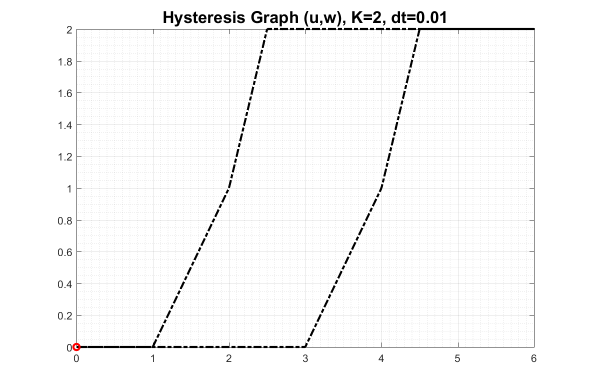
(a) $\Pi=[1,1,3,1;1,3,5,1]$	(b) $\Pi=[1,1,3,1;1,2,4,1]$	(c) $\Pi=[1,1,3,1;2,2,4,1/2]$
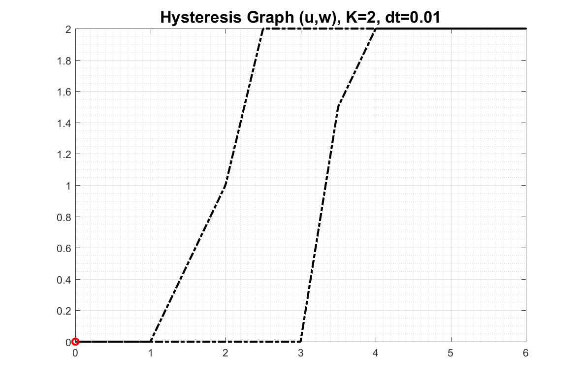
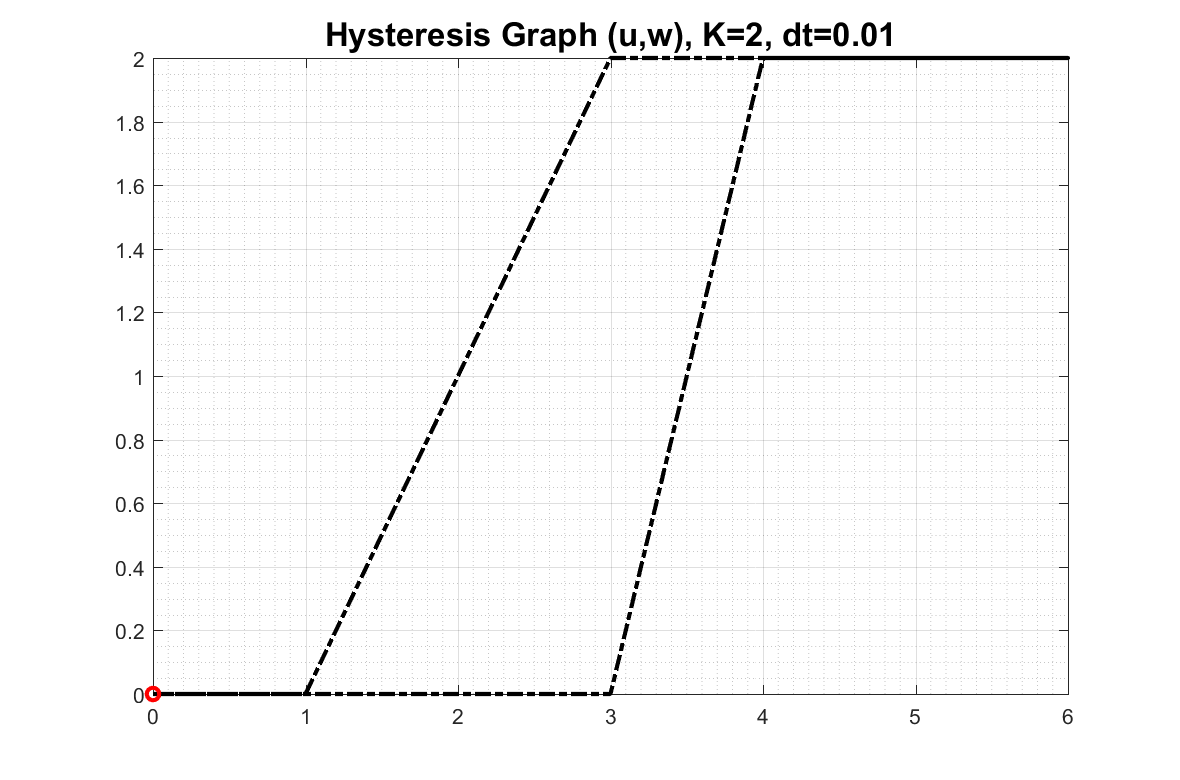
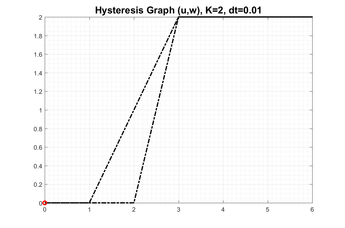
(d) $\Pi=[1,1,3,1;2,2,3,1/2]$	(e) $\Pi=[1,1,3,1;1,2,3,1]$	(f) $\Pi=[1,1,2,1;1,2,2,1]$

Figure 4: Examples of stacking $K=2$ hysterons in $K$-nonlinear play model. Shown is $H=(u,w)=\mathcal{H}(\Pi;u)$ with $\Pi$ as indicated and $u(t)=\mathcal{L}(0,6,0)$ in all cases.

3.3.1 Stacking $K$ hysterons for slopes of rational ratio

We continue case (e) from the previous example. Consider now some $m,n\in\mathbb{N}$ such that $r=\dfrac{m}{n}$ is irreducible. Consider $K=mn$ hysterons each with uniform $h_{k}=h,\mu_{k}=1$. Assume each of $\alpha_{k}$ and $\beta_{k}$ forms a non-decreasing set. The $\alpha_{k}$ are grouped as $m$ non-overlapping adjacent sets of $n$ points, and the $\beta$s are partitioned into $n$ non-overlapping adjacent sets of $m$ points:

$$\{\alpha_{1}=\dots=\alpha_{n}<\alpha_{n+1}=\dots=\alpha_{2n}<\dots<\alpha_{(m-1)n+1}=\dots=\alpha_{mn}\}$$ (25a)

$$\{\beta_{1}=\dots=\beta_{m}<\beta_{m+1}=\dots=\beta_{2m}<\dots<\beta_{(n-1)m+1}=\dots=\beta_{nm}\}$$ (25b)

These give slope $n$ on $[\alpha_{1},\alpha_{1}+mh]$, and slope $m$ on $[\beta_{1},\beta_{1}+nh]$. The output $H$ has the shape of trapezoid, with the side slopes of ratio $r$. Multiplying all by some factor $\mu$ gives arbitrary slopes $s_{l}$ on left and $s_{r}$ on right, but their ratio $\dfrac{s_{r}}{s_{l}}=r$. We call the resulting operator $\mathcal{H}(\Pi;u)$ a trapezoidal hysteron.

Definition 2.

$\mathcal{H}(\Pi;u)$ is called a trapezoidal hysteron if the primary curves in $H$ form a trapezoid whose top and bottom sides are parallel to the $u$-axis, and the left and right sides have positive slopes $s_{l},s_{r}$ with a rational ratio

$$\frac{s_{l}}{s_{r}}\in\mathbb{Q}.$$ (26)

The parameters $\alpha_{k},\beta_{k}$ satisfy (25), and $h_{k},\mu_{k}$ are uniform.

3.3.2 Comparison of $K$-Preisach model with $K$-nonlinear play

Finally we continue Example 3.3.1(e), and compare the resulting $\mathcal{H}(\Pi^{K,1};u)$ to that obtained with $K$-Preisach model; see Fig. 5, and calibration with monotone $\{\alpha_{k},\beta_{k}\}$. Since $K$ is finite, as expected, $\mathcal{H}(\Pi^{K,0};u)$ produces discontinuous output. With regularization with $b^{h}_{\varepsilon}$, the stair-step effect is diminished. With $\varepsilon=1$, the primary curves in $H$ for $\Pi^{K,0}$ are close to those for $\Pi^{K,1}$, but the secondary curves differ substantially.

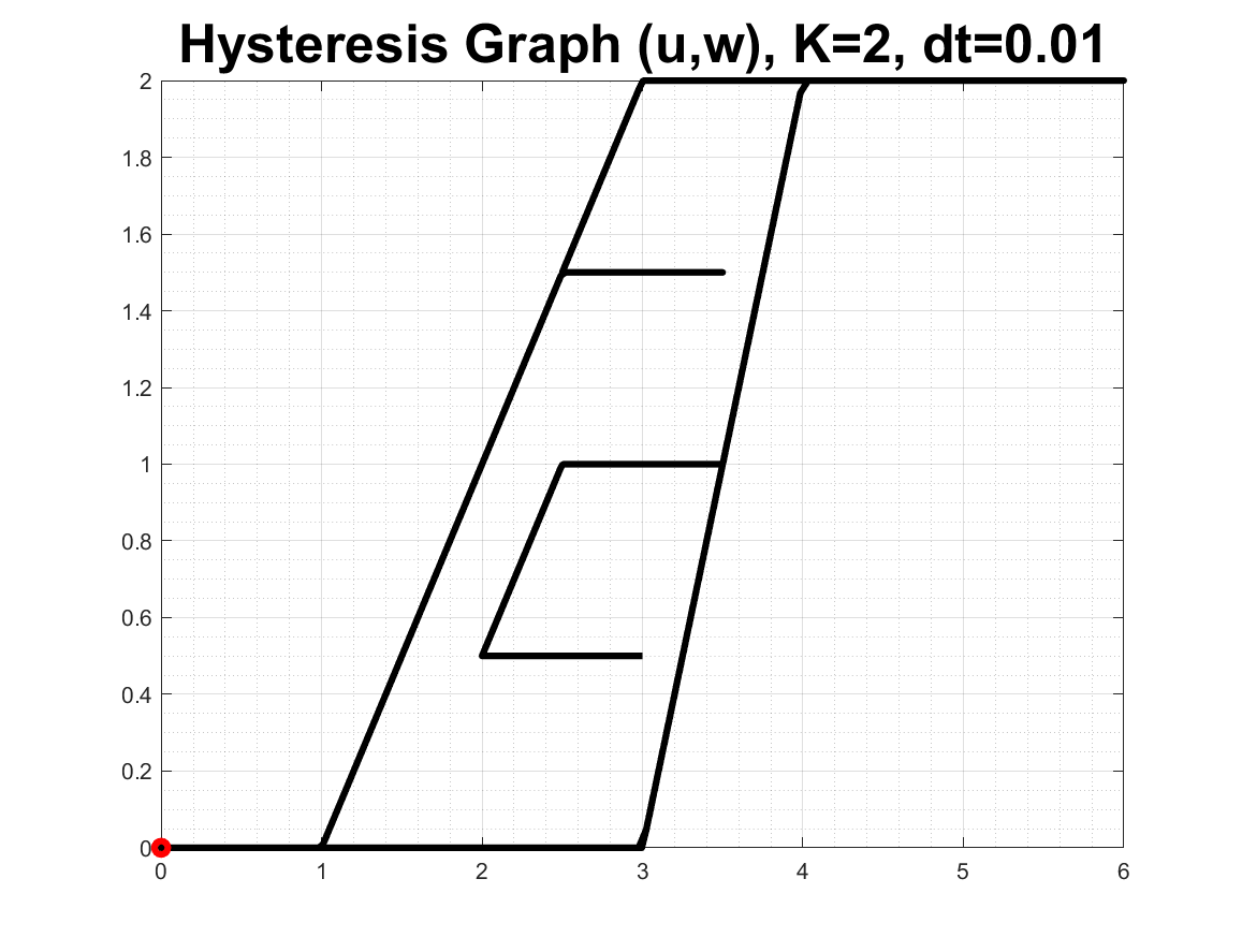
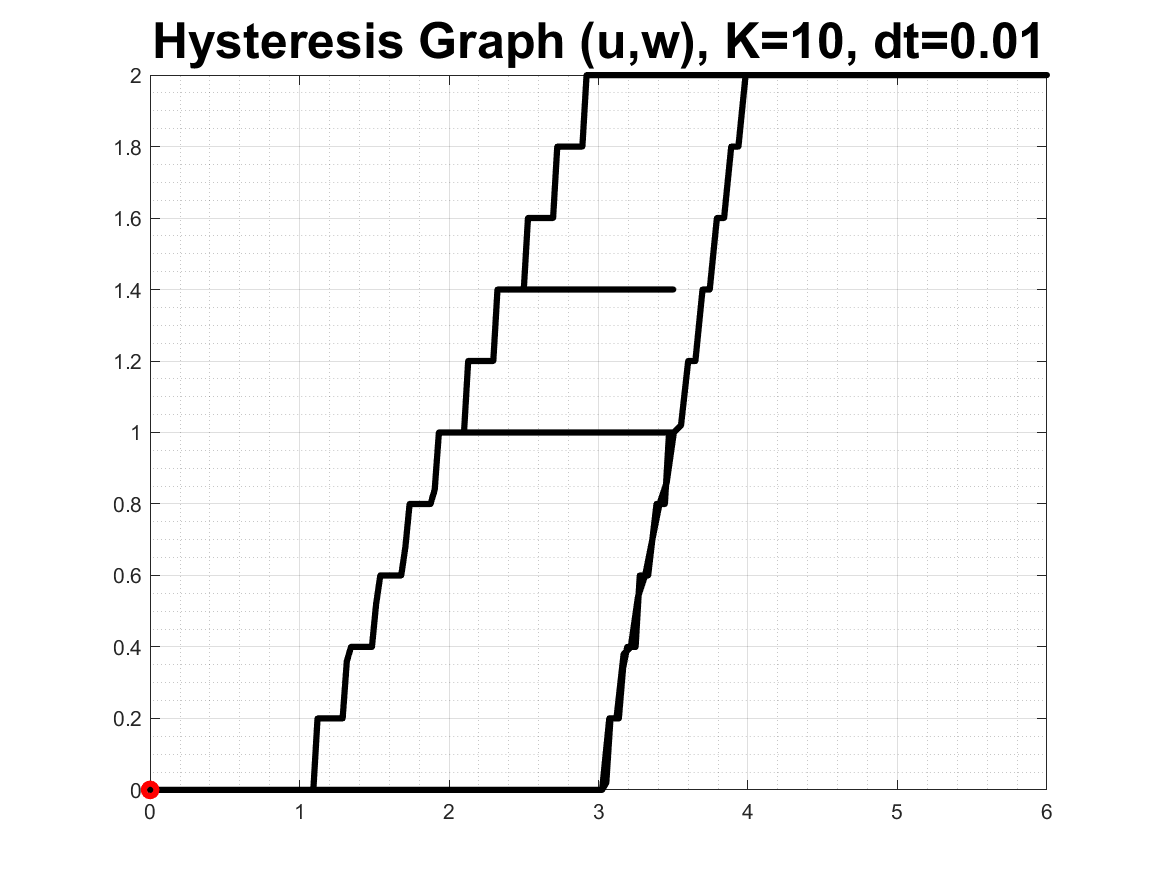
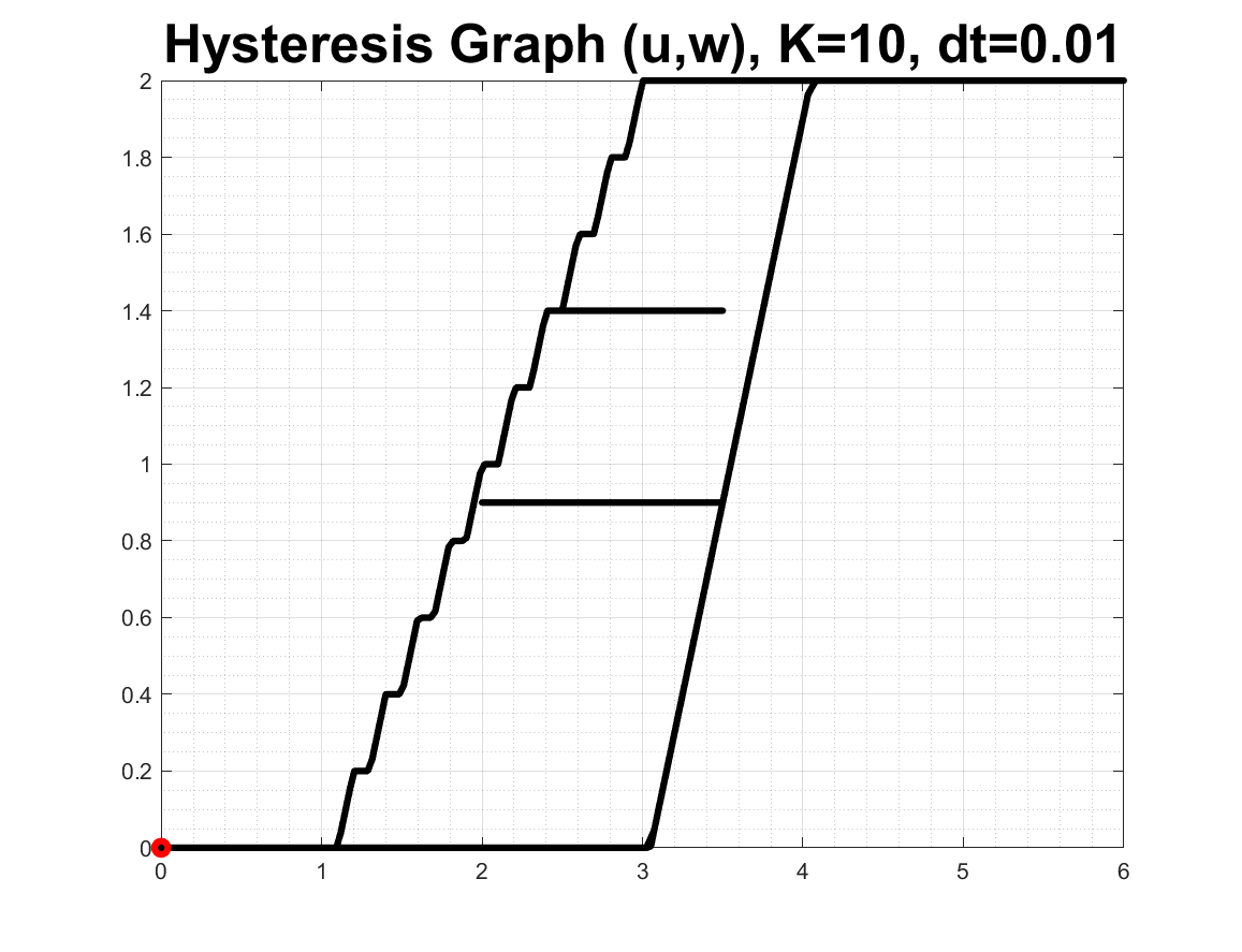
(a) $\Pi^{2,1}$	(b) $\Pi^{10,0}$	(c) $\Pi^{10,\varepsilon}$ with $\varepsilon=1/2$.

Figure 5: Comparison of $\mathcal{H}(\Pi;u)$ with $K$-nonlinear play and the $K$-Preisach model for the same trapezoidal hysteron $H$ as in Fig. 4 (e). We use ${\mathcal{U}}=[0,6,2.5,3,3.5,0,3.5,2,3]$ which more than sweeps $H$. (a) $K$-nonlinear playwith $\Pi^{2,1}=[1,1,3,1;1,2,3,1]$. (b): $K$-Preisach approximation is rough with $K=10$, and (c) smoother if $\Pi^{K,\varepsilon}$ is used. Note the richness of the secondary scanning curves in (a) and flatness in (b-c).

4 Calibration and approximation of hysteresis functionals

In this section we calibrate $\mathcal{H}$, i.e., we consider the “inverse problem”: Given some data $\mathcal{D}$ including $H$, find $\Pi^{*}$ so that

$$H\approx H^{*}=\mathcal{H}(\Pi^{*};u;v^{init}).$$ (27)

for any $u$ that sweeps $H$. We recall that the calibration process provided in literature for the Preisach model involves the so-called Preisach plane and requires $(u,w)\in\mathcal{D}$ with $u$ from a family of inputs dense in $C^{0}$. See, e.g., the contributions in [15, 25, 19].

Finding $\Pi^{K}_{\infty}$ is easy but only possible if $H$ is symmetric as indicated in Tab. 2. We show how to find $\Pi^{\gamma},\Pi^{K,0},\Pi^{K}_{\infty},\Pi^{K,1}$ for the same $H$. The algorithm for $K$-nonlinear play model is most involved, even if $H$ is a trapezoidal hysteron.

We assume below that $H$ is representable, i.e., that $H$ is a boundary of some $\mathcal{H}\subset\mathbb{R}^{2}=\{(u,w)\}$, a generalized trapezoid defined below.

Definition 3.

$H$ is a generalized trapezoid $H$ if it is a boundary of closed simply connected region $\mathcal{H}=\{(u,w)\}\subset\mathbb{R}^{2}$ satisfying the following. $H$ must have top and bottom sides parallel to the $u$ axis, and monotone lateral sides so that its boundary $H=bd(\mathcal{H})=H_{b}\cup H_{l}\cup H_{t}\cup H_{r}$ of $\mathcal{H}$ is made of, respectively, the bottom, left, top, and right bounding curves. We have

$$H_{b}=[\alpha,\beta]\times\{w_{min}\};\;\;H_{t}=[A,B]\times\{w_{max}\}$$

for given $\alpha,\beta,A,B,w_{min},w_{max}\in\mathbb{R}$ such that

$$0\leq\alpha\leq\beta,\;\;0\leq A\leq B,\;\alpha<A,\beta<B,\;0\leq w_{min}<w_{max},\;0<\frac{A-\alpha}{B-\beta}<\infty.$$ (28)

The left and right curves $H_{l}=(u,\gamma_{l}(u)),u\in[\alpha,A]$ and $H_{r}=(u,\gamma_{r}(u)),u\in[\beta,B]$, are the graphs of functions which are continuous piecewise smooth increasing and injective on $(\alpha,B)$. These functions either (i) coincide on all $[\alpha,B]$, or (ii) they satisfy

$$\gamma_{l}(u)>\gamma_{r}(u),\;u\in(\alpha,B);\;\mathrm{and}\;\;\gamma_{l}(u)\geq\gamma_{r}(u),\;u\in\{\alpha,B\}.$$ (29)

The curves $H_{l},H_{r}$ are the downward left curve and the upward right curve, respectively. For convenience we also list the vertices $vert(H)$ of $H$ in the counter-clockwise order

$$vert(H)=\{(\alpha,w_{min}),\;(\beta,w_{min}),\;(B,w_{max}),\;(A,w_{max})\}.$$ (30)

Finally, the data on $H$ might be given from experiment, i.e.,

$$\mathcal{D}=(u^{l}_{k},w_{k})_{k=1}^{K+1}\cup(u^{r}_{k},w_{k})_{k=1}^{K+1}$$ (31)

chosen so that $w_{k}=\gamma_{r}(u_{k}^{r})=\gamma_{l}(u_{k}^{l})$, with $u_{1}^{l}=\alpha,u^{l}_{K+1}=A,u^{r}_{1}=\beta,u^{r}_{K+1}=B$. Assume that $(u^{r}_{k})_{k}$ and $w_{k}$ are increasing sequences.

We note that some graphs which are not representable can be broken up into smaller pieces which are amenable to approximation. Further, if $H$ is non-hysteretic, i.e., $\alpha=\beta$, and $A=B$, it can be parametrized by a single unit hysteron. Lastly, if instead of (31), the data $\mathcal{D}=\mathcal{D}^{l}\cup\mathcal{D}^{r}=(u^{l}_{k},w^{l}_{k})_{k=1}^{K_{l}+1}\cup(u^{r}_{k},w^{r}_{k})_{k=1}^{K_{r}+1}$ with $K_{l}\neq K_{r}$ or $w^{l}_{k}\neq w^{r}_{k}$, then one must pre-process $\mathcal{D}$, e.g., by taking an intersection of $\mathcal{D}^{l}$ and $\mathcal{D}^{r}$ and interpolating.

Now we comment on the inputs $u(t)$. We say that the input $u(t)$ sweeps $H$ if $u:[0,T]=[0,T^{+}]\cup[T^{+},T]\to[\alpha,B]$ is an absolutely continuous function $u\in W^{1,1}[0,T)$ such that

$$u(0)=u(T)=\alpha;u(T^{+})=B;$$ (32a)

$$u^{\prime}(t)\geq 0,\;\mathrm{a.e.}\;\;t\in[0,T^{+}];\;\;u^{\prime}(t)\leq 0,\;\mathrm{a.e.}\;t\in[T^{+},T].$$ (32b)

We denote the set of such sweeping functions by $u\in\mathcal{S}(H)$. Typically we choose $u\in\mathcal{L}({\mathcal{U}})$ for some ${\mathcal{U}}$ that includes $\{\alpha,B,\alpha\}$.

4.1 Finding $\Pi^{\gamma}$ for generalized play

Calibration of $\Pi^{\gamma}$ does not take any effort. We take as $\gamma_{l}$ and $\gamma_{r}$ the functions whose graphs form $H_{l}$ and $H_{r}$. We record $\Pi^{\gamma}=[1,\gamma_{l}(\cdot),\gamma_{r}(\cdot),\mathrm{id}]$. If discrete experimental data is used, we can set $\gamma_{l}(\cdot),\gamma_{r}(\cdot)$ to be, e.g., piecewise linear interpolants of the data on $H_{l},H_{r}$, respectively.

4.2 Finding $\Pi^{K,0},\Pi^{K,\varepsilon},\Pi^{K,*}$ for $K$-Preisach models

Given $K$, we partition the range $[w_{min},w_{max}]$ into $K$ intervals, and form $K$ rectangles, each of height $h_{k}$ so that $\sum_{k}h_{k}=w_{max}-w_{min}$. It is easiest to choose uniform $h_{k}=h=(w_{max}-w_{min})/K$. Then we set $w_{k}=w_{min}+\sum_{j=1}^{k-1}h_{j},k=1,\ldots K+1$. For each $w_{k}$ we find $u^{l}_{k}=\gamma_{l}^{-1}(w_{k})$ and $u^{r}_{k}=\gamma_{r}^{-1}(w_{k})$. We see that $u^{l}_{1}=\alpha$, and $u^{l}_{K+1}=A$, while $u^{r}_{1}=\beta$, and $u^{r}_{K+1}=B$. Finally we set rectangles, each of height $h_{k}$, with left corner $\alpha_{k}=(u^{l}_{k}+u^{l}_{k+1})/2$ and $\beta_{k}=(u^{r}_{k}+u^{r}_{k+1})/2$. We record each $\Pi_{k}=[\infty,\alpha_{k},\beta_{k},h_{k}]$, and collect in $\Pi^{K,0}$. The output $u\to w=\mathcal{H}(\Pi^{K,0};u)$ will be discontinuous.

We can now choose some $\varepsilon$ for $\Pi^{K,\varepsilon}$, with each $\Pi_{k}$ replaced by $\Pi^{\varepsilon}_{k}=[1/\varepsilon,\alpha_{k},\beta_{k},\varepsilon h_{k}]$, with some small $\varepsilon$. The output $u\to w=\mathcal{H}(\Pi^{K,\varepsilon};u)$ will be continuous with intermittent flat pieces.

4.3 Finding $\Pi^{K}_{\infty}$ for $K$-linear play

For a $K$-linear play operator $u\to\mathcal{H}(\Pi;u)$ finding $\Pi$ requires only the knowledge of one of $H_{r}$ or $H_{l}$, since $H_{l}$ must be a symmetric reflection of $H_{r}$ with respect to the midpoint of $H$. For meaningful calibration we assume that the top and bottom parts of $H$ are single points where $H_{l}$ and $H_{r}$ intersect. To calibrate, wlog, we take $H_{r}$. For every interval $(u^{r}_{k},u^{r}_{k+1})$ we approximate the slope of $\gamma_{r}(\cdot)|_{(u^{r}_{k},u^{r}_{k+1})}$ with finite differences $s_{k}=\frac{w_{k+1}-w_{k}}{u^{r}_{k+1}-u^{r}_{k}}$. Next we set simply

$$\alpha_{k}=u_{1};\forall k;\;\beta_{k}=u_{k};\forall k;\;\mu_{1}=s_{1};\;\mu_{k}=s_{k}-\sum_{m=1}^{k-1}\mu_{m};k>1.$$

Since the weights $\mu_{k}$ approximate the second derivatives of $\gamma_{r}(\cdot)$, which is convex, we get $\mu_{k}\geq 0$; see [38] for more. The secondary curves of $K$-linear play $\mathcal{H}$ are not horizontal; rather, they have shape similar to that of translates of $\gamma_{l},\gamma_{r}$, with a rich structure completely determined by $\Pi^{K}_{\infty}$. This will be evident in examples in Sec. 4.6.3.

4.4 Finding $\Pi^{K,1}$ for $K$-nonlinear play

We start in Sec. 4.4.1 by describing how to parametrize $H$ when $H$ is a trapezoidal hysteron  as in Def. 2. We follow in Sec. 4.4.2 by a hierarchical algorithm which approximates any representable $H$ (as in Def. 3) with curvilinear sides, by a sum of trapezoidal hysterons.

4.4.1 Algorithm $H\approx H^{*}\to\Pi$ for trapezoidal hysteron $H$ with linear sides

Assume a trapezoid $H$ as in Def. 2, with vertices $vert(H)=\{(\alpha,\underline{w}),\;(\beta,\underline{w}),\;(B,\overline{w}),\;(A,\overline{w})\}.$ We calculate

$$h=\overline{w}-\underline{w};\;\gamma_{l}^{\prime}=s_{l}=\frac{h}{A-\alpha};\gamma_{r}^{\prime}=\frac{h}{B-\beta};\;r=\frac{s_{r}}{s_{l}}=\frac{A-\alpha}{B-\beta}.$$

We can set $K=mn$ and calculate $\Pi=(\Pi_{k})_{k=1}^{K}\in\mathbb{R}^{K\times 4}$ with simple formulas given below. However, we can also approximate $\mathbb{Q}\ni r^{*}=\tfrac{m^{*}}{n^{*}}\approx r$, with a new $K^{*}=m^{*}n^{*}\ll K$. This is useful when $r\not\in Q$, i..e, (26) does not hold, or when $K=mn$ is impractically large. The approximation $r\approx r^{*}$ now gives a new $H^{*}\approx H$ with $vert(H)\approx vert(H^{*})$. The parameters $\Pi^{*}$ for $H^{*}$ are found with the calculations below.

(STEP (a)) Approximate $r$ by an irreducible fraction $r\approx r^{*}=\frac{m^{*}}{n^{*}}\in\mathbb{Q}.\;\mathrm{Set\ }K^{*}=m^{*}n^{*}$.

(STEP (b)) Choose the new slopes $s_{l}^{*}\approx s_{l},s_{r}^{*}\approx s_{r}$ of the sides of $H^{*}$. The choice of $s_{l}^{*}$ and $s_{r}^{*}$ is not unique, but we require $r^{*}=\frac{s_{r}^{*}}{s_{l}^{*}}$. Once $s_{l}^{*}$ and $s_{r}^{*}$ are set, calculate the points $A^{*},B^{*}$, the scaling factor $\mu^{*}$ and the subinterval length $h^{*}$, $A^{*}=\alpha+\frac{h}{s_{l}^{*}};B^{*}=\beta+\frac{h}{s_{r}^{*}};\mu^{*}=s_{l}^{*}m^{*}=s_{r}^{*}n^{*};h^{*}=\frac{h}{\mu^{*}}.$ For example, we can set $s_{l}=s_{l}^{*}$, and use $s_{r}^{*}=s_{l}r^{*}$, $\mu^{*}=s_{l}{m^{*}}$, and $A^{*}=A$ and $B^{*}=\beta+\frac{h}{s_{r}^{*}}$. Alternatively, we can set $s_{r}^{*}=s_{r}$, $s_{l}^{*}=\frac{s_{r}^{*}}{r^{*}}$, with $\mu^{*}={s_{r}}{n^{*}}$, $B^{*}=B$ and $A^{*}=\alpha+\frac{h}{s_{l}^{*}}$. Other options are possible.

(STEP (c)) With $\mu^{*}$, and $h^{*}$ known, set $\mu_{k}=\frac{\mu^{*}}{K^{*}};\;\;h_{k}=h^{*};\;\;k=1,\ldots K^{*}.$

(STEP (d)) Define $\alpha_{k},\beta_{k}$, enumerating $1\leq k\leq K^{*}$ as $k=(j-1)n+l$ or $k=(l-1)m+j$.

$$\alpha_{(j-1)n+l}=\alpha+(j-1)h^{*};\;\beta_{(l-1)m+j}=\beta+(l-1)h^{*};\;1\leq j\leq m,\;\;1\leq l\leq n.$$

In the end we collect $\Pi^{*}$ with $H^{*}=\mathcal{H}(\Pi^{*};u),u\in\mathcal{S}(H)$. In particular, we require

$$vert(\mathcal{H}^{*})=\{(\alpha,\underline{w}),\;(\beta,\underline{w}),\;(B^{*},\overline{w}),\;(A^{*},\overline{w})\},$$ (33)

satisfy (28), and that $\mid\!A-A^{*}\!\mid+\mid\!B-B^{*}\!\mid\approx 0$ and $H_{l}\approx H_{l}^{*}$ and $H_{r}\approx H_{r}^{*}$.

Remark 1.

Given $r\in\mathbb{R}$, the choice of irreducible fraction $r^{*}\approx r$ is not unique. To maintain accuracy, i.e., to minimize $\mid\!r-r^{*}\!\mid$, we use diophantine approximations, e.g., with the MATLB function rat with desired accuracy [26]. To constrain the magnitude of $K^{*}=m^{*}n^{*}$, we consider some $K^{max}$ and search for $m^{*},n^{*}$

$$(m^{*},n^{*})=\mathrm{argmin\ }_{(m,n):mn\leq K^{max}}\left|\frac{m}{n}-r\right|^{2}.$$ (34)

In practice, it suffices to search in $[1,\sqrt{K^{max}}]^{2}$, with $K^{max}=O(100)$.

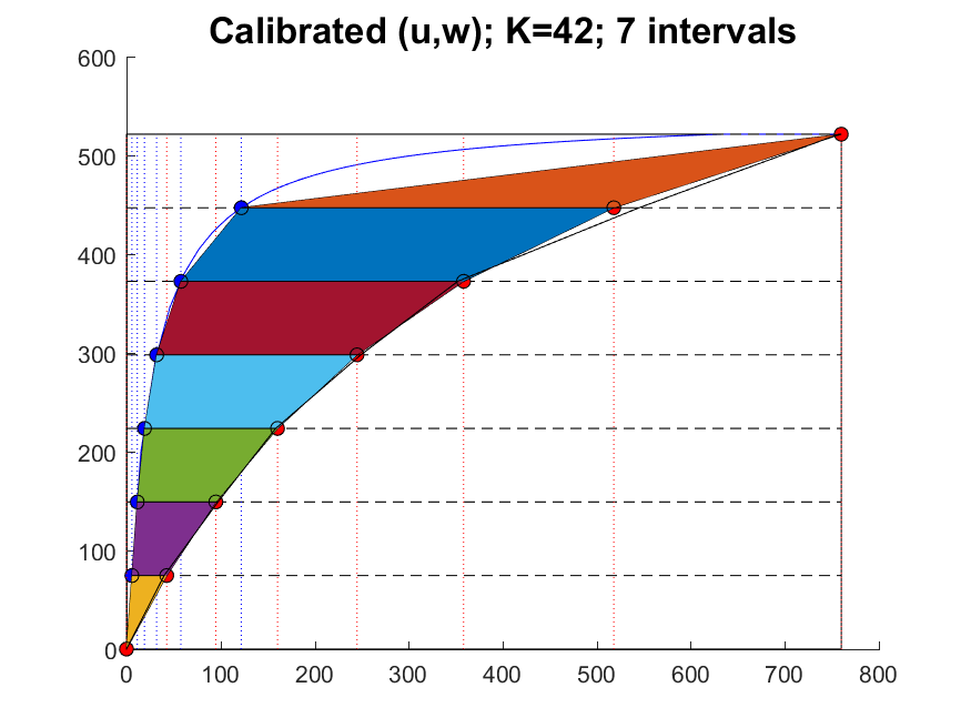
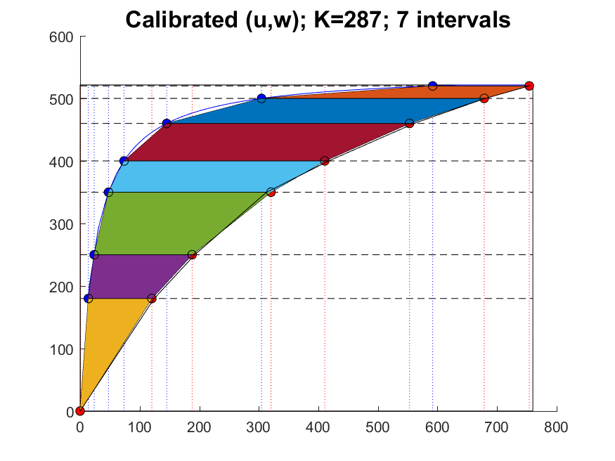
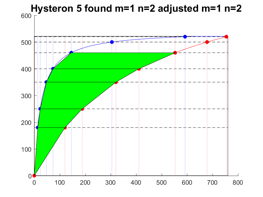
(a)	(b)	(c)

Figure 6: Calibration for adsorption hysteresis graph, with $H$ made of $\gamma_{l}$ curve (in blue) and $\gamma_{r}$ (in red), with original $H$ as shown in Fig. 2 (a). Partition of the range into $I=7$ intervals is the first step in the calibration with $\Pi^{K,1}$, with the corresponding trapezoidal hysterons filled in. (a) With a uniform partition, some portions of $\mathcal{H}$ are inadequately covered. (b) An adaptively chosen partition gives a better approximation $H^{*}\approx H$ and better coverage of $\mathcal{H}$. The $K$-nonlinear play graph is found for (a) with $K=42$ and (b) $K=287$, respectively. (c) For the adaptive vertical partition, the individual trapezoidal hysterons are found step by step. The step $i=6$ (with $K_{6}=2$) is shown, with the trapezoidal hysterons $\mathcal{H}_{1},\mathcal{H}_{2}\ldots\mathcal{H}_{i-1}$ filled with green.

4.4.2 Hierarchical approach for $H$ with general shape in Def. 3

We approximate $H\approx H^{*}$ and cover $\mathcal{H}$ by a union of $I$ trapezoidal hysterons with a process illustrated in Fig. 6. The key is the partition $w_{min}=w_{0}<w_{1}<\ldots w_{I}=w_{max}.$ of the range $[w_{min},w_{max}]$ of $\mathcal{H}$ into $I$ subintervals which can be, in principle, arbitrary. We isolate the partitions

$$\mathcal{H}_{i}=\mathcal{H}\cap\{(u,w)\in\mathcal{H}:w_{i-1}\leq w\leq w_{i}\}$$

of $\mathcal{H}$. The boundary $H_{i}$ of each graph $\mathcal{H}_{i}$ has the top and bottom sides parallel to the $u$-axis, with the height at most $h_{I}=\max_{i}(w_{i}-w_{i-1})$. The curvilinear left and right sides of $H_{i}$ follow the curves $(u,\gamma_{l}(u))$ and $(u,\gamma_{r}(u))$, respectively, and the vertices of $H_{i}$

$$vert(H_{i})=\{(\alpha_{i},w_{i-1}),(\beta_{i},w_{i-1}),(B_{i},w_{i}),(A_{i},w_{i})\};\;\alpha_{i}=(\gamma_{l})^{-1}(w_{i-1}),\beta_{i}=(\gamma_{r})^{-1}(w_{i-1})$$

are well defined. The continuity of $\gamma_{r},\gamma_{l}$ requires

$$A_{i}=\alpha_{i+1},\;\;B_{i}=\beta_{i+1},\;\;0\leq i\leq I-1.$$ (35)

If the $i^{\prime}$th portion of the graph is not hysteretic, we have $\alpha_{i}=\beta_{i}$, and $A_{i}=B_{i}$. If the sides of each $H_{i}$ are linear and satisfy (26), we find some $\Pi_{i}=(\Pi_{k_{i}})_{k_{i}=1}^{K_{i}}$ for each $H_{i}$, and collect $\Pi=((\Pi_{k_{i}})_{k_{i}=1}^{K_{i}})_{i=1}^{I}$ renumbered appropriately. However, if the sides are not linear, or if (26) does not hold, or if $\sum_{i}K_{i}$ is too large, we proceed by iteration to satisfy the accuracy and efficiency needs, while we maintain continuity as in (35). An example of such iterative algorithm is given in the Appendix 8.1.

4.5 Quality of approximation $H\approx H^{*}$

The efforts to approximate a given $H\approx H^{*}$ are not much different from those of piecewise interpolation of the sides $H_{l},H_{r}$ of $H$. Once $\Pi^{*}$ is calibrated, the model $u\to w\in\mathcal{H}(\Pi^{*};u)$ can be coupled to some external dynamics, e.g., to ODE or PDE. However, then an additional modeling error arises since the actual accuracy of output $(u(t),w(t))\in\mathcal{H}$ depends on the accuracy of approximation of $u(t)$ and $w(t)$ by some $(U_{\tau},W_{\tau})$ in these other equations coupled to $u\to\mathcal{H}(\Pi;u)$.

With a large number $K$ of components $v_{k}$, the error in $u$ and $w$ would seem to accumulate in $w-W_{\tau}$ from that for the individual components $v_{k}-V_{k,\tau}$, and would affect $u-U_{\tau}$. However, for all models except $K$-linear play, the effect of the accumulation seems insignificant in practice, and a large $K$ is not an issue for accuracy of time-stepping, but may be desired to reduce model error $H-H^{*}$. At the same time, large $K$ requires more computational time.

Finally when discussing $H\approx H^{*}$, we must realize that in practice we encounter ($U^{*}_{\tau},W^{*}_{\tau})\in\mathcal{H}_{\tau}(\Pi^{*};u^{*}_{\tau})$. The modeling error $H\approx H_{\tau}^{*}$ contributes to the global approximation error $u-U_{\tau}^{*}$, and $w-W_{\tau}^{*}$.

4.6 Examples of $K$-nonlinear play, $K$-Preisach and $K$-linear play models

4.6.1 Trapezoid with curvilinear sides

Consider first $H^{lin}$ with $vert(H^{lin})=\{(3,0),(9,0),(11,5),(4,5)\}$ and linear sides. The slopes of these sides are $s_{l}=5$, $s_{r}=\frac{5}{2}$, with $h=5$, and $r=\frac{s_{l}}{s_{r}}=\frac{1}{2}$, We accept $H^{*}=H^{lin}$, and set $m^{*}=m=1,n^{*}=n=2$, with $K^{*}=2$, and calculate $h^{*}=\frac{A-\alpha}{m^{*}}=1$, $\mu^{*}=\frac{h}{h^{*}}=5$. Each $\mu_{k}=\frac{\mu^{*}}{K^{*}}=\frac{5}{2}$, and $h_{k}=h^{*}=1$. We summarize $\mathcal{H}(\Pi^{lin};\cdot)$ with $\Pi^{lin}=[\frac{5}{2},3,9,1;\frac{5}{2},3,10,1]$.

Consider now curvilinear hysteresis graph $\mathcal{H}$ with $vert(H)=\{(3,0),(9,0),(B,5),(4.1,5)\}$, and $B=11+\tfrac{\pi}{10}$. The left side of $\mathcal{H}$ is given by the quadratic polynomial $\gamma_{l}(u)=\frac{50}{11}(x-3)+\frac{1}{2}[(x-3.55)^{2}-0.55^{2}]$, while $\gamma_{r}(u)$ is the piecewise linear function which connects the vertices $(9,0)$ and $(B,5)$. To find an approximation $\mathcal{H}^{*}$, we proceed by iteration. We set $q=0$ and $vert(H^{(0)})=\{(3,0),(9,0),(B,5),(4.1,5)\}.$ Here the linear left side of $H^{(0)}$ with the slope $s_{l}=\frac{50}{11}$ does not match very well the primary scanning curve in $H$. We also see that $s_{r}$ in exact precision is not rational, thus we continue.

In iteration $q=1$ we consider a trapezoidal hysteron $\mathcal{H}^{(1)}$ associated with

$$vert(H^{(1)})=\{(3,0),(9,0),(B^{(1)},5),(4.1,5)\},$$

with the double prevision decimal approximation $B^{(1)}=11.314159265358979\approx B$. We have $r^{(1)}\approx\tfrac{11}{23.14159265358979}$. We can find $m^{(1)},n^{(1)}$ so that $r^{(1)}\in\mathbb{Q}$. However, the corresponding $K^{(1)}=O(10^{16})$, very large and impractical. We try next $vert(H^{(2)})$, setting $B^{(2)}=11.3$, with $vert(H^{(2)})=\{(3,0),(9,0),(11.3,5),(4.1,5)\}.$ Now $r^{(2)}=\frac{11}{23}$. We set $m^{(2)}=11$, $n^{(2)}=23$, and parametrize $H^{(2)}$ with $K^{(2)}=mn=253$ unit hysterons. In particular, we have $h^{*}=\frac{1.1}{11}=\frac{1}{10}$, and $\mu^{*}=50$, while each $\mu_{k}=\frac{50}{11\cdot 23}$, and each $h_{k}=h^{*}$. We number the unit hysterons with $k=(j-1)n+l$ or $k=(l-1)m+j$ when $1\leq j\leq 11,1\leq l\leq 23$. In particular, $\alpha_{1}=\ldots\alpha_{23}=\alpha=3$, but $\alpha_{24}=3+h^{*}$, and $\alpha_{253}=\alpha+10h^{*}=4$. In turn, $\beta_{1}=\beta_{24}=\beta=9$ but $\beta_{2}=\beta+h^{*}$, and $\beta_{253}=\beta+22h^{*}=9+2.2=11.2$. We get

139150253239.1150253…243.19150253…253411.2150253superscriptΠ2fragments 139150253239.1150253…missing-subexpressionmissing-subexpressionmissing-subexpressionmissing-subexpression243.19150253…missing-subexpressionmissing-subexpressionmissing-subexpressionmissing-subexpression253411.2150253\displaystyle\Pi^{(2)}=\begin{tabular}[]{|l|ll|ll|}\hline\cr$k$&$\alpha_{k}$&$\beta_{k}$&$h_{k}$&$\mu_{k}$\\ \hline\cr 1&3&9&1&$\tfrac{50}{253}$\\ 2&3&9.1&1&$\tfrac{50}{253}$\\ \ldots&&&&\\ 24&3.1&9&1&$\tfrac{50}{253}$\\ \ldots&&&&\\ 253&4&11.2&1&$\tfrac{50}{253}$\\ \hline\cr\end{tabular}

kαkβkhkμkkαkβkhkμk (43)

However, $K^{(2)}$ may be still too large to be practical, and we try again. Setting $B^{(3)}=11.2$ we have $\frac{s_{r}}{s_{l}}=\frac{1}{2}$ and we can set $m^{*}=1,n^{*}=2$. The parametrization of $vert(H^{(3)})=\{(3,0),(9,0),(11.2,5),(4.1,5)\}.$ is similar to that for $H^{lin}$. The difference is the new scaling factor $\mu^{*}=\frac{50}{11}$, and $h^{*}=\frac{11}{10}$. The individual scaling factor for each unit hysteron is now $\mu_{k}=\frac{25}{11}$. We set $\mathcal{H}^{*}(u)=\mathcal{H}(\Pi^{(3)};u)$, with

1391.125112310.11.12511superscriptΠ3fragments 1391.125112310.11.12511\displaystyle\Pi^{(3)}=\begin{tabular}[]{|l|ll|ll|}\hline\cr$k$&$\alpha_{k}$&$\beta_{k}$&$h_{k}$&$\mu_{k}$\\ \hline\cr 1&3&9&1.1&$\frac{25}{11}$\\ 2&3&10.1&1.1&$\frac{25}{11}$\\ \hline\cr\end{tabular}

kαkβkhkμkkαkβkhkμk (47)

4.6.2 Same trapezoid, two ways.

A given trapezoidal hysteron can be parametrized in more than one way. Let $vert(H)=\{(4,0),(8,0),(8,1),(10,1)\}$ and $H$ have linear sides, with the corresponding $\frac{s_{r}}{s_{l}}=2$. We can use $I=1$ or $I=4$ and the parametrizations

148214268214,Π8= 1480.51424.580.514358.50.51445.58.50.5145690.51466.590.514779.50.51487.59.50.514fragments fragments148214268214superscriptΠ8fragments 1480.51424.580.514358.50.51445.58.50.5145690.51466.590.514779.50.51487.59.50.514\displaystyle\begin{tabular}[]{|l|ll|ll|}\hline\cr$k$&$\alpha_{k}$&$\beta_{k}$&$h_{k}$&$\mu_{k}$\\ \hline\cr 1&4&8&2&$\frac{1}{4}$\\ 2&6&8&2&$\frac{1}{4}$\\ \hline\cr\end{tabular},\;\;\Pi^{8}=\begin{tabular}[]{|l|ll|ll|}\hline\cr$k$&$\alpha_{k}$&$\beta_{k}$&$h_{k}$&$\mu_{k}$\\ \hline\cr 1&4&8&0.5&$\frac{1}{4}$\\ 2&4.5&8&0.5&$\frac{1}{4}$\\ 3&5&8.5&0.5&$\frac{1}{4}$\\ 4&5.5&8.5&0.5&$\frac{1}{4}$\\ 5&6&9&0.5&$\frac{1}{4}$\\ 6&6.5&9&0.5&$\frac{1}{4}$\\ 7&7&9.5&0.5&$\frac{1}{4}$\\ 8&7.5&9.5&0.5&$\frac{1}{4}$\\ \hline\cr\end{tabular}

$$\Pi^{2} = \begin{tabular}[]{|l|ll|ll|}\hline\cr$k$&$\alpha_{k}$&$\beta_{k}$&$h_{k}$&$\mu_{k}$\\ \hline\cr 1&4&8&2&$\frac{1}{4}$\\ 2&6&8&2&$\frac{1}{4}$\\ \hline\cr\end{tabular},\;\;\Pi^{8}=\begin{tabular}[]{|l|ll|ll|}\hline\cr$k$&$\alpha_{k}$&$\beta_{k}$&$h_{k}$&$\mu_{k}$\\ \hline\cr 1&4&8&0.5&$\frac{1}{4}$\\ 2&4.5&8&0.5&$\frac{1}{4}$\\ 3&5&8.5&0.5&$\frac{1}{4}$\\ 4&5.5&8.5&0.5&$\frac{1}{4}$\\ 5&6&9&0.5&$\frac{1}{4}$\\ 6&6.5&9&0.5&$\frac{1}{4}$\\ 7&7&9.5&0.5&$\frac{1}{4}$\\ 8&7.5&9.5&0.5&$\frac{1}{4}$\\ \hline\cr\end{tabular}$$ kαkβkhkμkkαkβkhkμkkαkβkhkμkkαkβkhkμk (60)

Here $\Pi^{8}$ is obtained with a uniform partition of $[0,1]$ to $\{w_{0},w_{1},w_{2},w_{3},w_{4}\}=\{0,0.25,0.5,0.75,1\}$, and Algorithm in Sec. 4.4.2 yields $K=8$ unit hysterons, each with $h^{*}=0.5$. Denote by $[r]$ the integer part of $r$. We have ${\mathcal{H}^{*}}(\Pi^{8};\cdot)=\sum_{k=1}^{8}\mathcal{H}(\tfrac{1}{4},{4+\tfrac{k-1}{2},8+\tfrac{[k-1/2]}{2}},h^{*};\cdot)$. In other words, both $\Pi^{2}$ and $\Pi^{8}$ yield the same bounding curves in $H$. Since it is more efficient to have $K=2$ than $K=8$, model $\Pi^{2}$ is preferable over $\Pi^{8}$. We note that even though $H(\Pi^{2})=H(\Pi^{8})$, the operator $\mathcal{H}(\Pi^{2})\neq\mathcal{H}(\Pi^{8})$ since the images $\mathcal{H}(\Pi^{2};u)\neq\mathcal{H}(\Pi^{8};u)$ when $u\not\in\mathcal{S}(H)$.

4.6.3 Smooth graph with $K$-linear play model, $K$-Preisach model, and $K$-nonlinear play model

Now let $H$ be symmetric convex-concave, with $\gamma_{r}(u)=(u-1)^{2}+1/3(u-1)$. The left curve is obtained on $[u_{min},u_{max}]$ by symmetric reflection with $\gamma_{l}(u)=\gamma_{r}(u_{max})-\gamma_{r}(u_{min}+u_{max}-u)$.

We compare the output for generalized play, with $\Pi^{\gamma}$, the $K$-linear play model, $K$-nonlinear play, and $K$-Preisach. Fig. 7 illustrates $\mathcal{H}(\Pi;u)$ obtained for a particular $u\in\mathcal{L}({\mathcal{U}})$ with ${\mathcal{U}}$ designed to sweep $H$ as well as to show a few secondary loops.

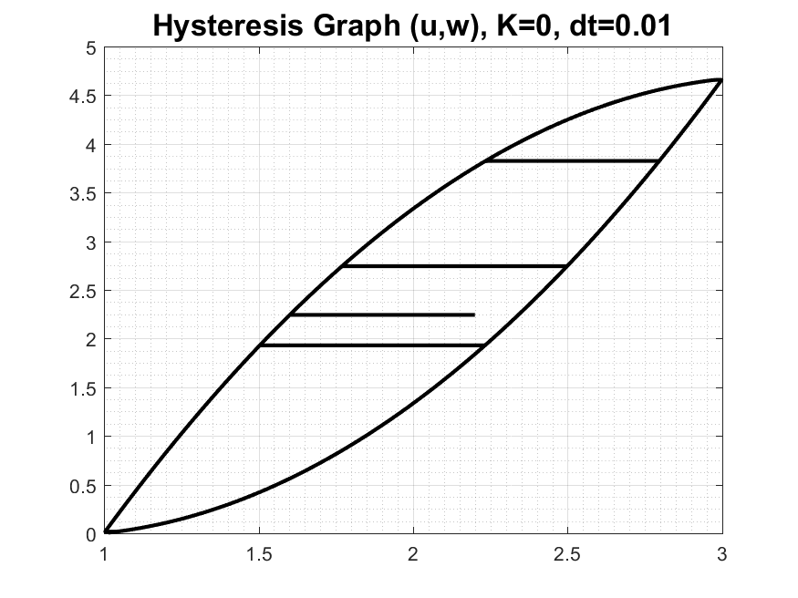
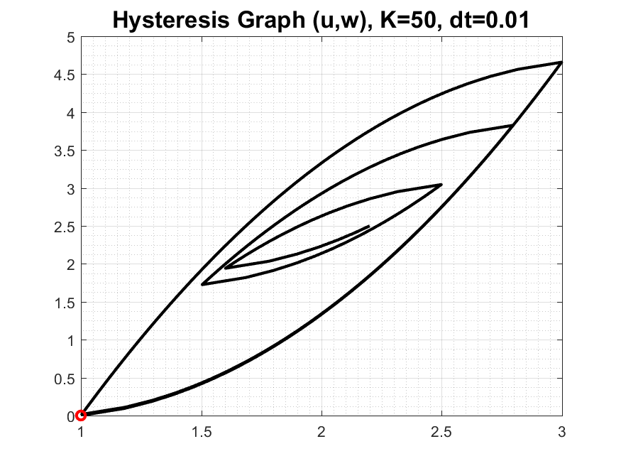
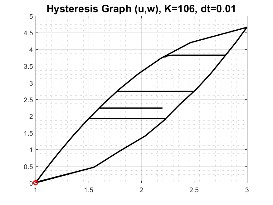
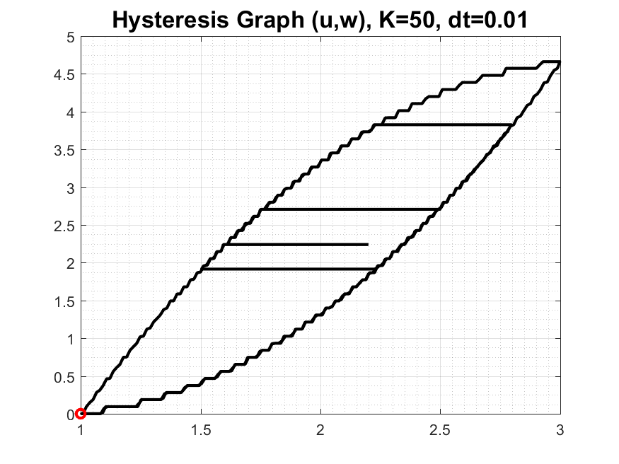
generalized	$K$-linear play	$K$-nonlinear play	$K$-Preisach
$\Pi^{\gamma}$	$\Pi^{K}_{\infty}$, $K$=50	$\Pi^{K,1}$, $K$=106	$\Pi^{K,\varepsilon}$, $K$=50, $\varepsilon=1/10$

Figure 7: Hysteresis graph with $K$-linear play for a smooth curve $\gamma_{r}(u)=(u-1)^{2}+1/3(u-1)$. Note the richness of interior loops with $K$-linear play model with $\Pi^{K}_{\infty}$. Here ${\mathcal{U}}=[1,3,1,2.8,1.5,2.5,1.6,2.2]$.

4.6.4 Adsorption-desorption hysteresis graph from experimental data

Now we calibrate hysteresis functional $\mathcal{H}(\Pi;\cdot)$ for realistic experimental adsorption–desorption data for methane CH4 from [18]. This data is fit in [18] to a particular algebraic model called Langmuir isotherm $\gamma(u)=V\tfrac{Bu}{1+Bu}$ for each of the desorption $\gamma_{l}(u)$ and adsorption $\gamma_{r}(u)$ curves, respectively. The data is given in Tab. 3.

	V	B
adsorption, $\gamma_{r}(\cdot)$	811	0.00237
desorption, $\gamma_{l}(\cdot)$	543	0.0382

Table 3: Data for the Langmuir fit of the adsorption-desorption curves in Sec. 4.6.4.

We use this data to produce $H$ and calibrate $\mathcal{H}(\Pi;)$ with generalized play, $K$-nonlinear play and $K$-Preisach models. For $K$-nonlinear play, we consider $I=7$ trapezoidal hysterons with a uniform partition or an adaptive partition, both shown in Fig. 6, with the corresponding $K=42$ and $K=287$. The latter adheres more closely to $H$, and seems a better model in spite of a large $K$. See Fig. 8 for illustration.

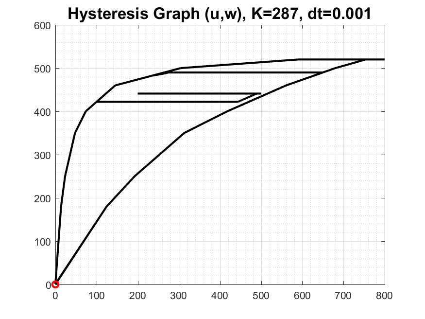
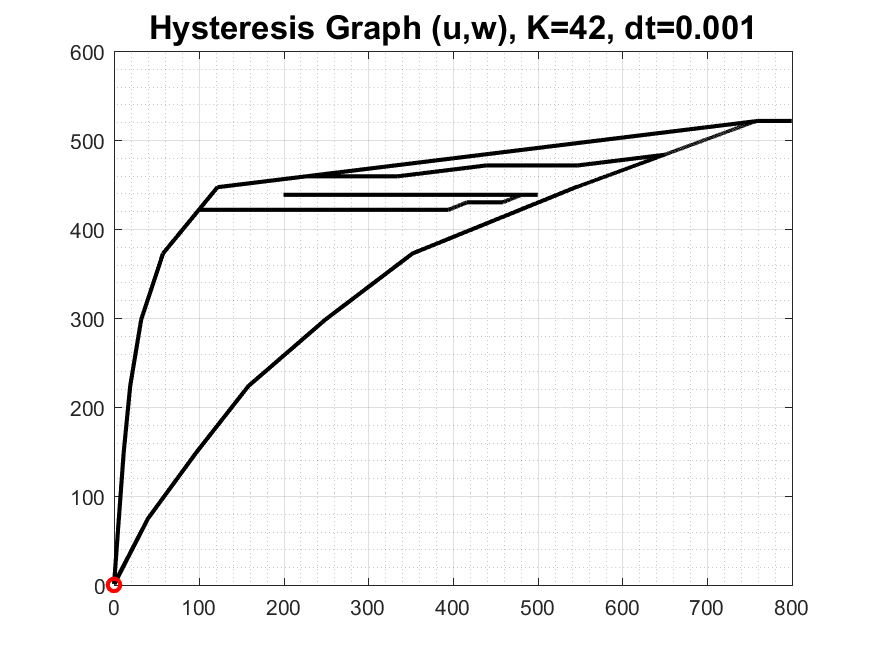
generalized	$K$-nonlinear play	$K$-nonlinear play	$K$-Preisach
$\Pi^{\gamma}$	$\Pi^{K,1}$, adaptive, $K=287$	$\Pi^{K,1}$, uniform, $K=42$	$\Pi^{K,\varepsilon}$, $K=50$,$\varepsilon=1/10$

Figure 8: Comparison of hysteresis graphs for the CH4 adsorption-desorption curves from [18] $\mathcal{H}$ plotted with ${\mathcal{U}}=[0,800,0,650,100,350,500,200]$. The $K$-linear play model is not available since $H$ is not symmetric. The graphs can be compared to those in Fig. 2. Note that the graph for $\Pi^{\gamma}$ is annoted specially with $K=0$.

5 Analysis of evolution with $K$-generalized play hysteresis

To discuss the well-posedness of (1) with hysteresis, and to prove stability of the numerical scheme, we first formulate some auxiliary results for the stationary problem for the related system

$$\tfrac{d}{dt}(a(u)+b(v)) = f,$$ (61a)

$$\tfrac{d}{dt}b(v)+\mathcal{C}(\gamma_{r}(u),\gamma_{l}(u);v) \ni 0.$$ (61b)

The system (61) corresponds to (1) with $A=0$ and generalized play $\mathcal{H}(u)=\mathcal{H}(\Pi^{\gamma};u)$ obtained from the solution to the initial-value problem (5). Our results extend those we proved in [39] for $K$-nonlinear play.

We start by writing (61) in the form

$$\tfrac{d}{dt}a(u)-\xi = f,\quad\xi\in\mathcal{C}(\gamma_{r}(u),\gamma_{l}(u);v),$$ (62a)

$$\tfrac{d}{dt}b(v)+\xi \ni 0.$$ (62b)

We prove properties of (62) with $K$-generalized play in Sec. 5.1, which we later use in Sec. 6.1 for the numerical schemes for (61).

Note that for each $u\in\mathbb{R}$ the graph $\mathcal{C}(\gamma_{r}(u),\gamma_{l}(u);\cdot)$ is maximal monotone, and for each $v\in\mathbb{R}$ the graph $-\mathcal{C}(\gamma_{r}(\cdot),\gamma_{l}(\cdot);v)$ is maximal monotone. This is the form which occurs in the coupling with PDEs to give well-posed initial-value problems in the space $L^{1}\times L^{1}$ for systems such as (61). We will add to (61a) an appropriate operator $A$ in $L^{1}$ for the PDE, and in Sec. 5.2 we use these towards the statement on well-posedness of (1); later we use these to show the stability of an implicit-explicit numerical scheme for (1) when $A$ is an advection-diffusion operator in $L^{1}$. Both the well-posedness results for these systems as well as estimates for their discrete approximations depend on these results.

5.1 Estimates for (62)

Implicit-difference approximations of (62) lead to consideration of the following systems.

Lemma 4.

If assumptions (6) hold, then solutions $(u,v)$ and $(\bar{u},\bar{v})$ of

$$a(u)-\xi=f,\ b(v)+\xi=b(g),\ \xi\in\mathcal{C}(\gamma_{r}(u),\gamma_{l}(u);v),$$ (63a)

$$a(\bar{u})-\bar{\xi}=\bar{f},\ b(\bar{v})+\bar{\xi}=b(\bar{g}),\ \bar{\xi}\in\mathcal{C}(\gamma_{r}(\bar{u}),\gamma_{l}(\bar{u});\bar{v}),$$ (63b)

satisfy the estimates

$$(a(u)-a(\bar{u}))^{+}+(b(v)-b(\bar{v}))^{+}\leq(f-\bar{f})^{+}+(b(g)-b(\bar{g}))^{+},$$ (64)

and

$$|a(u)-a(\bar{u})|+|b(v)-b(\bar{v})|\leq|f-\bar{f}|+|b(g)-b(\bar{g})|.$$ (65)

Proof.

Subtract the respective equations,

$$(a(u)-a(\bar{u}))-(\xi-\bar{\xi})=f-\bar{f},\ (b(v)-b(\bar{v}))+(\xi-\bar{\xi})=b(g)-b(\bar{g}),$$

multiply by $\operatorname{sgn}_{0}^{+}(u-\bar{u})$ and then $\operatorname{sgn}_{0}^{+}(v-\bar{v})$ and add to obtain

$$(a(u)-a(\bar{u}))^{+}+(b(v)-b(\bar{v}))^{+}+(\xi-\bar{\xi})\big{(}\operatorname{sgn}_{0}^{+}(v-\bar{v})-\operatorname{sgn}_{0}^{+}(u-\bar{u})\big{)}\leq(f-\bar{f})^{+}+(b(g)-b(\bar{g}))^{+}.$$

Below we verify the third term is non-negative, so we obtain (64). The corresponding estimates hold for the negative parts $(\cdot)^{-}$ and then for their sum, (65). This shows the solution is order-preserving.

Finally, we check that $(\xi-\bar{\xi})\big{(}\operatorname{sgn}_{0}^{+}(v-\bar{v})-\operatorname{sgn}_{0}^{+}(u-\bar{u})\big{)}\geq 0$. If $u=\bar{u}$ or $v=\bar{v}$ it is $\geq 0$ by the monotonicity of $\mathcal{C}$ in each variable. Otherwise consider the displacement $(u-\bar{u},v-\bar{v})$ in each quadrant of $\mathbb{R}\times\mathbb{R}$ with $(u,v)$ on the constraint and $(\bar{u},\bar{v})$ in the interior. In the first quadrant this term is $(\xi-\bar{\xi})(1-1)$ and in the third it is $(\xi-\bar{\xi})(0-0)$. In the second it is $(\xi-0)(1-0)\geq 0$ and in the fourth quadrant it is $(\xi-0)(0-1)\geq 0$. ∎

Corresponding results hold as well for K-generalized play as given by (21).

Proposition 1.

Assume in (21) that for each $1\leq k\leq K$, the functions $a(\cdot),b_{k}(\cdot),\gamma_{l,k},\gamma_{r,k}$ satisfy (6). Then the solutions $(u,v),\ v=(v_{k})$ and $(\bar{u},\bar{v}),\ \bar{v}=(\bar{v}_{k})$ of the respective systems

$$a(u)-\sum_{k=1}^{K}\xi_{k}=f,\ b_{k}(v_{k})+\xi_{k}=b_{k}(g_{k}),\ \xi_{k}\in\mathcal{C}(\gamma_{rk}(u),\gamma_{\ell k}(u);v_{k}(t)),\ 1\leq k\leq K,$$ (66a)

$$a(\bar{u})-\sum_{k=1}^{K}\bar{\xi}_{k}=\bar{f},\ b_{k}(\bar{v}_{k})+\bar{\xi}_{k}=b_{k}(\bar{g}_{k}),\ \bar{\xi}_{k}\in\mathcal{C}(\gamma_{rk}(\bar{u}),\gamma_{\ell k}(\bar{u});\bar{v}_{k}(t)),\ 1\leq k\leq K,$$ (66b)

with data $(f,g),\ g=(g_{k})\in\mathbb{R}^{K}$ and $(\bar{f},\bar{g}),\ \bar{g}=(\bar{g}_{k})$ satisfy the estimates

$$(a(u)-a(\bar{u}))^{+}+\sum_{k=1}^{K}(b_{k}(v_{k})-b_{k}(\bar{v}_{k}))^{+}\leq(f-\bar{f})^{+}+\sum_{k=1}^{K}(b_{k}(g_{k})-b_{k}(\bar{g}_{k}))^{+},$$ (67)

and

$$|a(u)-a(\bar{u})|+\sum_{k=1}^{K}|b_{k}(v_{k})-b_{k}(\bar{v}_{k})|\leq|f-\bar{f}|+\sum_{k=1}^{K}|b_{k}(g_{k})-b_{k}(\bar{g}_{k})|.$$ (68)

This follows from the same proof as in Lemma 4 with the corresponding estimates $(\xi_{k}-\bar{\xi}_{k})(\operatorname{sgn}_{0}^{+}(v_{k}-\bar{v}_{k})-\operatorname{sgn}_{0}^{+}(u-\bar{u}))\geq 0$ for $1\leq k\leq K$.

The results hold also when $\gamma_{l,k},\gamma_{r,k}$, are permitted to be maximal monotone relations without common points of multiple-values. See [55] (VIII.2).

5.2 PDE coupled to Hysteresis

Now we consider the evolution equation (1) in which $\mathcal{H}(\cdot)$ is a generalized play given by (21) and $A$ is a PDE on a domain $\Omega$ for advection or diffusion with appropriate boundary conditions. For the case of generalized play, the equation takes the form of the system (61) with $A$ added to the first equation. The estimates in Lemma 4 show that the operator $\mathcal{C}$ on $\mathbb{R}\times\mathbb{R}$ given by $(a(u),b(v))\to(-\xi,\xi)$ with $\xi\in\mathcal{C}(\gamma_{r}(u),\gamma_{l}(u);v)$ is accretive. This is the analogue of monotone on a Banach space $B$, and with the range condition $\operatorname{Rg}(I+\mathcal{C})=B$ it is called m-accretive. If $\mathcal{C}$ is m-accretive, $v^{init}\in\overline{\operatorname{Dom}(\mathcal{C})}$, and $f\in L^{1}(0,T;B)$, then the initial-value problem (8) has a unique integral solution. This is a limit in $C([0,T];B)$ of implicit-difference approximations (9). For Banach spaces which possess the Radon-Nikodym property, in particular, for finite-dimensional spaces, if $f$ has bounded total variation, the integral solution is a strong solution $v\in W^{1,\infty}(0,T;B)$; see [55] (XII.4).

Corresponding estimates for the system in the product space $B=L^{1}(\Omega)\times L^{1}(\Omega)$ show the initial-value problem for (62) is well posed, that is, it has a unique integral solution in $C([0,T];B)$. The same is true with $A(u)$ added to the first equation if $A$ is accretive on $L^{1}(\Omega)$. Moreover the same argument with Proposition 1 extends to the other forms of play hysteresis and we obtain the following general result. See [55] (VIII.3) and [54, 29, 39].

Proposition 2.

Assume the conditions (6) and that $A$ is m-acretive on the Banach space $L^{1}(\Omega)$. Then the initial-value problem for (1) with $\mathcal{H}$ as in (21), under (22), is well posed. In particular, it holds when $\mathcal{H}(\cdot)$ is either generalized play with $\Pi^{\gamma}$ or $K$-nonlinear play with $\Pi^{K,1}$ or regularized $K$-Preisach (with $\Pi^{K,\varepsilon}$ or $\Pi^{K,*}$).

6 Numerical scheme for an ODE and PDE with hysteresis

Now we discuss some practical challenges when solving numerically a dynamical problem involving $\mathcal{H}(\cdot)$. Numerical models with hysteresis were discussed and analyzed in [52, 53, 14], all for Preisach type models and parabolic PDEs. Here we use different techniques motivated by explicit schemes for transport.

We define first an implicit numerical scheme for the ODE (61) and discuss its solvability, solver, and convergence rate. Next we consider (1) with an advective transport $A(u)$. We apply an Ex-Im scheme (explicit-implicit) in which the PDE term $A(u)$ is treated first explicitly in time, followed by an implicit solver for the hysteresis accumulation term $u+w$ with the scheme for the ODE (61).

6.1 Numerical scheme for ODE (61)

We approximate $(u,w)$ solving (61) with $w\in\mathcal{H}(\Pi^{K};u)$. We seek $(U^{n},W^{n})$ defined by

$$a(U^{n})-a(U^{n-1})+W^{n}-W^{n-1} = \tau F^{n},$$ (69a)

Here we set $$F^{n}=f(t_{n}) f F^{n}=\tfrac{1}{\tau}\int_{t_{n-1}}^{t_{n}}f(s)ds W^{n} U^{n} V^{n}=(V^{n}_{k})_{k} v_{k} w=b(v)$$ for smooth , or otherwise. Next we need as a function of ; we also seek which approximate solving (16), and solving (18). For these we have a unified formula (24), and we have

$$W^{n}={\mathcal{G}}(\Pi;V^{n-1};U^{n})=\sum_{k=1}^{K}\mu_{k}b_{k}(\mathcal{R}_{k}(V^{n-1}_{k};U^{n})).$$ (69b)

The function ${\mathcal{G}}(\Pi;\overline{V};U)$ has properties which extend from these of each $\mathcal{R}_{k}$ and of $b_{k}$. In particular, these are the monotonicity properties expressed in Lemmas 1 and 2. From these the next result follows.

Lemma 5.

The solution $(U^{n},W^{n})$ to (69) exists and is unique.

Proof.

We substitute $W^{n}$ from (69b) into (69a) to obtain the stationary problem for $U^{n}$

$$a(U^{n})+{\mathcal{G}}(\Pi;V^{n-1};U^{n})=a(U^{n-1})+W^{n-1}+\tau F^{n}.$$ (70)

Since $a(\cdot)+{\mathcal{G}}(\Pi;\overline{V};\cdot)$ is monotone strictly increasing, with range $\mathbb{R}$, this equation has a unique solution $U^{n}$. Once $U^{n}$ is known we calculate $(V^{n}_{k})_{k}$ and $W^{n}$ from (69b). ∎

We also prove additional properties. They are analogues of what was proven in [39] for $K$-nonlinear play. We only need to prove the counterparts of [39] (Lemma 4.4) and [39] (Prop.4.5). We also need an additional result similar to that in [39] (Prop.4.6).

Lemma 6.

The solutions to (69) satisfy

$$\mid\!a(U^{n})-a(U^{n-1}\!\mid+\sum_{k}\mu_{k}\mid\!b_{k}(V_{k}^{n})-b_{k}(V_{k}^{n-1})\!\mid=\tau\mid\!F^{n}\!\mid.$$ (71)

Proof.

The lemma was proved for $K$-nonlinear play model in [39]. It remains to verify (71) for $\Pi=\Pi^{\gamma}$ and $\mathcal{H}(\Pi;\cdot)$ represents the $K$-generalized play model. We recall Lemma 1. From this monotonicity result we can write $W_{k}^{n}-W_{k}^{n-1}=\mu_{k}b_{k}(V_{k}^{n})-\mu_{k}b_{k}(V_{k}^{n-1})=\psi_{k}(U^{n}-U^{n-1})$ with some $\psi_{k}\geq 0$; this is similar to the use of mean value theorem, but we need not identify $\psi_{k}$ with a derivative. Similarly, we also have $a(u)-a(\overline{u})=\chi(u-\overline{u})$, with positive $\chi\geq 0$. Thus (69a) is equivalent to

$$(\chi+\sum_{k}\psi_{k})(U^{n}-U^{n-1})=\tau F^{n},$$

Next, $F\geq 0$ implies $U^{n}-U^{n-1}\geq 0$, and $F\leq 0$ implies $U^{n}-U^{n-1}\leq 0$, thus we obtain the desired result. ∎

6.2 Implementation, solver, and convergence of discrete scheme (69)

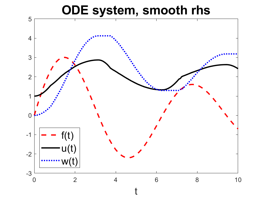
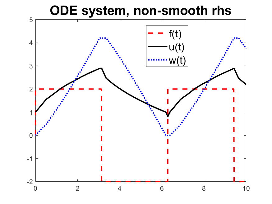
(a)	(b)
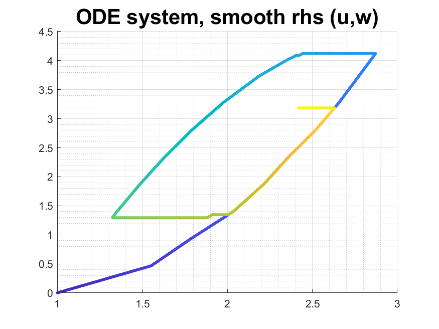
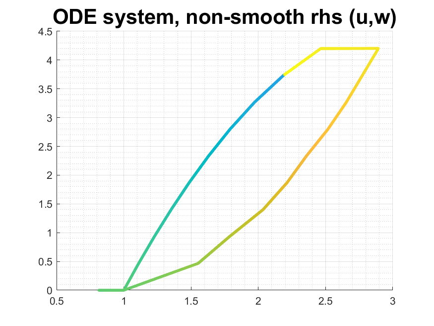
(c)	(d)

Figure 9: Illustration of ODE with hysteresis with $\Pi^{K,1}$ from Sec. 4.6.3. Top: $f(t),U_{\tau},W_{\tau}$ for (a) $f=f^{cont}$ and (b) $f=f^{disc}$, and $\tau=10^{-4}$. Bottom: (c) the trace $(U^{n},W^{n})_{n}$ of $\mathcal{H}(\Pi^{K,1};)$ for (c) $f=f^{cont}$ and (d) $f=f^{disc}$.

We discuss how the solution to (69) is found in practice. We set-up an example for (61) with $\mathcal{H}(\Pi;\cdot)$ for the convex–concave graph $H$ from Sec. 4.6.3 and $\Pi$ as one of $\Pi^{\gamma},\Pi^{K}_{\infty},\Pi^{K,1},\Pi^{K,\varepsilon}$. We use $u^{init}=1$, a compatible $v^{init}$, and the source function as one of the two

$$T=10;\;\;f^{cont}(t)=3.5\mathrm{sin}(t)e^{-0.1t};\;f^{disc}(t)=\mathrm{sign}(f^{cont}(t)).$$ (72)

The experiment is designed so that $(U_{\tau},W_{\tau})$ for both $f^{cont}$ and $f^{disc}$ loop almost all over $H$; see Fig. 9. Here $U_{\tau},W_{\tau}$ are the piecewise linear interpolants of $(U_{n})_{n}$ and $(W_{n})_{n}$, respectively.

6.2.1 Solver for (69a)

Since (70) is a scalar root-solving problem on $\mathbb{R}$, there are many excellent solvers. Newton’s method uses derivative information and converges fast close to the root [20] whenever the residual is a smooth function of $u$. However, Newton’s method may have occasional difficulty handling only piecewise differentiable functions such as ${\mathcal{G}}(u)$. In this (semismooth) case [51] the solver still may converge, but with occasional failures. A robust alternative is a method we call Root which brackets the root and then uses a secant method [7]; this method is implemented in fzero in MATLAB. The Root solver is robust but also much slower than Newton iteration. Both require an implementation of the calculation for ${\mathcal{G}}(U^{n})$; Newton solver also requires its derivative.

We test solver performance. Of interest is the average $N_{ave}$ number of iterations as well as the computational time shown in Table 4. For perspective we show the case without hysteresis, which still requires a nonlinear solver at every time step $n$.

Solver	Root			Newton
case/$\tau$	0.1	0.01	0.001	0.1	0.01	0.001
$\gamma_{l}$=$\gamma_{r}$	9.31 (0.171)	7.33 (1.01)	7.1782 (9.44)	3.68 (0.117)	3 (0.583)	3 (5.29)
$\Pi^{\gamma}$
$f^{cont}$	9.08 (0.218)	8.15 (1.057)	8.602 (10.49)	3.29 (0.113)	2.79 (0.529)	2.78 (4.776)
$f^{disc}$	10.27 (0.174)	8.97 (1.135)	9.50 (11.21)	3.73 (0.124)	2.98 (0.590)	2.97 (5.059)
$\Pi^{K,1}$
$K$=$106$	7.98 (1.066)	7.14 (8.954)	7.94 (98.61)	2.42 (0.56)	2.07 (4.58)	2.01 (47.40)
$K$=$921$	9.01 (8.93)	7.7 (77.14)	8.46 (861.2)	2.98 (5.12)	2.09 (36.31)	2.01 (380.8)
$\Pi^{K}_{\infty}$
$K$=$50$	8.88 (0.455)	7.11 (3.54)	7.731 (39.65)	3.07 (0.34)	1.15 (1.87)	2.02(19.07)
K=200	9.67 (1.63)	7.58 (15.26)	8.08 (167.4)	3.08 (1.12)	2.47 (8.90)	2.04 (78.19)
$\Pi^{K,\varepsilon}$
$K$=$100$	14.35 (1.56)	11.92 (13.07)	11.48 (132.92)	–	–	–
$b^{h}_{*}$	10.08 (1.23)	8.63 (10.19)	9.39 (113.04)	3.78 (0.84)	3.014 (6.54)	2.98 (67.09)

Table 4: Solver performance for scheme (69) and experiments in Sec. 6.2. The numbers tabulated are the number of iterations and the computational time (in parentheses). The first row presents the case without hysteresis. The second two rows compare the use of $\Pi^{\gamma}$ for $f^{cont}$ and $f^{disc}$. Examples with $\Pi^{K,1},\Pi^{K}_{\infty},\Pi^{K,\varepsilon}$ are reported for the more challenging $f^{disc}$. Newton solver does not converge for some time steps when $\Pi=\Pi^{K,\varepsilon}$, unless regularization with $b^{h}_{*}$ is used.

The results in the Table show that the $\Pi^{K,\varepsilon}$ model is the most sensitive to the solver choice, while $\Pi^{\gamma}$ and $\Pi^{K}_{\infty}$ require the least amount of computational effort. As usual, when Newton converges, it converges faster than the Root solver. We use similar convergence criteria for both, with a combination of absolute ($10^{-14}$) and relative ($10^{-6}$) tolerance. As usual, smaller $\tau$ decreases somewhat the number of iterations, but overall the computational effort scales roughly linearly with the number of time steps. Newton solver performs poorly for the $K$-Preisach model, even though it can be made to work upon regularization.

The computational time for $K$-generalized play model is not significantly higher than that for case without hysteresis, and so is the number of iterations. As expected, higher $K$ requires more computational time than lower $K$, and the effort scales about linearly with $K$; compare, e.g., the $\Pi^{K}_{\infty}$ case with $K=50$ to that with $K=200$.

	$\Pi^{\gamma}$				$\Pi^{K,1}$	$\Pi^{K,1},b^{h}_{*}$
	$f^{cont}$		$f^{disc}$		$f^{cont}$	$f^{disc}$
$\tau$	$E_{u}$	$E_{w}$	$E_{u}$	$E_{w}$	$E_{u}$	$E_{u}$
0.1	0.0669978	0.108278	0.111336	0.134983	0.0592	0.10087
0.01	0.0068853	0.011001	0.010153	0.008205	0.00710	0.014807
0.001	0.0006917	0.001092	0.002179	0.003043	0.00065	0.001316

Table 5: Error $E_{u}=\mid\!\mid\!u-U_{\tau}\!\mid\!\mid\!_{\infty}$ and $E_{w}=\mid\!\mid\!w-W_{\tau}\!\mid\!\mid\!_{\infty}$ for the experiments in Sec. 6.2 with $\Pi$ from Sec. 4.6.3. We use the fine grid solution $(U_{\tau_{fine}},W_{\tau_{fine}})$ with $\tau_{\infty}=0.0001$ as a proxy for the true solution, and run the experiments for several $\tau$; some are shown here. We seek the order $p$: $E_{u}=O(\tau^{p})$. For the smooth source $f^{cont}$, we get $p\approx 1$ for $\Pi^{K,1}$ or $\Pi^{K}_{\infty}$ ($p=0.98$), but less dependably so when $f^{disc}$ is used. In fact, for $\Pi^{K,1}$ it is necessary to use additional smoothing $b^{h}_{*}$ or of $f^{disc}$ to achieve $O(\tau)$ convergence, at least within reasonable range of $\tau$.

6.2.2 Convergence rate for $\mid\!\mid\!u-U_{\tau}\!\mid\!\mid\!_{\infty}\to 0$ found in (69)

Table 5 is devoted to the rate. Generally, if $u\in W^{1,1}$ then $v\in W^{1,1}$ as well, and so is $w=b(v)$. However, it is not clear what to expect for $(u,w)$ solving (61). For nonsmooth $f$ such as $f=f^{disc}$, we expect $u+w\in W^{1,1}$, but the regularity of each $u(t)$ and $w(t)$ remains unclear. Since the analytical solution is not known, we use the fine grid solution.

While generally we expect about linear rate of convergence $O(\tau)$ in $u$, this expectation is not easy to confirm for graphs with large $K$, or even for $\Pi^{\gamma}$, within the range of practical time steps. As concerns $W$, the error seems stable, but we do not expect or always observe convergence, except for very simple $\Pi$.

6.3 Numerical scheme and analysis for a PDE

We now consider the homogeneous IVP which specializes (1) to when $A=\partial_{x}(\alpha(\cdot))$.

$$\tfrac{\partial}{\partial t}\left(a(u)+w\right)+\tfrac{\partial}{\partial x}\alpha(u) = 0,\;\;u(x,0)=u_{init}(x)\,;v(x,0)=v^{init}(x)\;\;$$ (73a)

$$w(x,t) = \mathcal{H}(u(x,t))$$ (73b)

The scheme we use is Ex-Im: explicit in the transport, with upwind treatment of advection, and implicit in the resolution of the nonlinearity under $\tfrac{\partial}{\partial t}$. For a spatial grid parameter $h$, we define the gridpoints $x_{j}=jh$ on the support of $u^{init}$, we set $U^{0}_{j}=u^{init}(x_{j})$, $V^{0}_{j,k}=v^{init}_{k}(x_{j})$, and at every time step $n>0$ we solve for $U_{j}^{n}\approx u(x_{j},t^{n})$ and $W_{j}^{n}\approx w(x_{j},t^{n})$ as follows:

$$\tfrac{1}{\tau}\left(a(U_{j}^{n})-a(U_{j}^{n-1})+W_{j}^{n}-W_{j}^{n-1}\right)+\tfrac{1}{h}(\alpha(U_{j}^{n-1})-\alpha(U_{j-1}^{n-1}))=0;$$ (74a)

$$W_{j}^{n}=\sum_{k}\mu_{k}b_{k}(\mathcal{R}_{k}(V_{k,j}^{n-1};U_{j}^{n})).$$ (74b)

Rearranging, we see that at every $n$ and $j$, one has to solve for $(U_{j}^{n},W_{j}^{n})$ a problem analogous to (69a) with $F^{n}_{j}=-\tfrac{\tau}{h}(\alpha(U_{j}^{n-1})-\alpha(U_{j-1}^{n-1}))$.

We have the following result on weak $TV_{T}$ stability of (74). We state it with a brief proof.

Proposition 3.

Assume the CFL condition $0\leq\tfrac{\tau}{h}\max_{u}\tfrac{d\alpha}{du}\leq 1$. The scheme (74) is uniquely solvable, and is weakly $TV_{T}$ stable in the $L^{1}\times(L^{1})^{K}$ space. Namely, $TV_{T}(a(U),(W_{k})_{k})\leq C(T)$ where the constant $C(T)$ depends on time $T$ but not on $\tau,h$.

Proof.

The proof for $\Pi=\Pi^{K,1}$ is given in [39] and relies on the properties of solvability ([39], Prop.4.5), comparison principle ([39], Lemma 4.4), and ordering ([39], Prop.4.6). The proof for general play requires that we verify properties listed above. These are, respectively, Lemma 5, Lemma 4, and Lemma 6 proven in this paper. ∎

The stability result combined with the usual truncation error analysis [27, 50] which is fairly simple for this upwind scheme suggest that the convergence rate $\mid\!\mid\!u-U_{h,\tau}\!\mid\!\mid\!_{1}$ is first order in $h$ or less, if the solutions are not smooth. We confirm this below. The error in $w$ is a different matter, since $w$ is only evaluated as a function of $u$. In fact, this evaluation may incur a local $O(\tau)$ modeling error since the manner of scanning the actual $\mathcal{H}(\Pi;\cdot)$ is dependent on the discretization error. So while $\mid\!\mid\!w-W_{h,\tau}\!\mid\!\mid\!_{1}$ remains stably bounded, in our experiments it is $O(1)$. The issue is similar to that discussed in Sec. 6.2.2.

6.4 Numerical examples for transport with hysteresis

We illustrate and compare the different hysteresis models for (1) with the scheme from Sec 6.3. The operator $\mathcal{H}(\Pi;\cdot)$ is constructed from either the symmetric concave-convex graph $H$ from Sec. 4.6.3, or from the adsorption–desorption graph from Sec. 4.6.4. We set $a(u)=u$ and $\alpha(u)=u$ in all examples, and focus on the hysteresis models alone; there is no substantial difficulty, but the exposition for more general functions $a(\cdot)$ and $\alpha(\cdot)$ takes more time.

We recall that the convergence rate was demonstrated to be $O(\sqrt{h})$ for $K$-nonlinear play case in [39], and essentially first order for $K$-linear play on examples similar to those presented below. We present here the case with generalized play shown in Table 6 which reveals that the order in $u$ is $O(h)$ for generalized play model. However, even though the solutions $W_{h,\tau}$ appear to visually converge, the error in $w$ scales like $O(1)$.

	h	0.01	0.005	0.001	0.0005
$\Pi^{\gamma}$, $u^{init}$ from Fig. 10	$E_{h}$	19.3351	10.0101	2.6699	1.32687	$p=0.89$
	h	0.05	0.01	0.005	0.001
$\Pi^{K,1}$, $u^{init}$ from Fig. 10	$E_{h}$	63.0521	17.7914	8.4411	1.3292	$p=0.98$
$\Pi^{K,1}$, $u^{init}$ from Fig. 11	$E_{h}$	28.70	2.96	2.72	0.08	$p=1.4$

Table 6: Error $E_{h}=\mid\!\mid\!u-U_{h,\tau}\!\mid\!\mid\!_{1}$ for (74), with $\Pi^{\gamma}$ and $\Pi^{K,1}$ for the adsorption model from Sec. 4.6.4, and initial conditions as indicated We use $\tau=0.9h$. The solution for $h_{fine}=0.0001$ and $h_{fine}=0.0005$ is a proxy for $u(x,t)$ for $\Pi^{\gamma}$ and $\Pi^{K,1}$ with $K=287$. The error for $w$ which is stable but appears $O(1)$is not shown. The error in $w$ is as shown, with roughly first order for all cases.

6.4.1 Transport with adsorption–desorption hysteresis from Sec. 4.6.4

We consider (73) with two different $v^{init}(x)$ as shown in Fig. 10 and Fig. 11. The first is made of a superposition of Riemann problems, the second is a simple piecewise linear.

The first case in Fig. 10 is designed to show how the solution $U_{h,\tau}\approx u(x,t)$ develops several interesting features. Since $\tau=h$ exactly, there is little diffusion and the fronts are not overly smeared. First, we observe the shock and rarefaction waves forming for the no-hysteresis case when suing $\gamma_{l}(u)$ and $\gamma_{r}(u)$. Since both of these are concave, the resulting function is convex, thus the fronts form in the front and rarefaction in the back, with the profile for $\gamma_{l}(\cdot)$ with steeper slopes travelling faster than that for $\gamma_{r}(\cdot)$. Then we turn to study the profile of $(U_{h,\tau},W_{h,\tau})$ corresponding to $\Pi=\Pi^{\gamma}$. Because the back of the first “box”drops almost discontinuously from $u=700$ down to $u=350$, the resulting $w$ follows a secondary scanning curve with slope $0$, as expected for the generalized hysteresis. Thus the resulting flux function is linear, and thus this part of the graph does not develop a smooth rarefaction, unlike for $\gamma_{l}$ or $\gamma_{r}$. For the input between $200\leq\leq 300$, $w$ follows again $\gamma_{l}(w)$ and the rarefaction develops again. The “trace” of the graph $(U_{j}^{n},W_{j}^{n})_{j,n})_{j,n}$ over all $j$ and $n$ from the entire simulation shows rather sparse sampling of $H$ due to discontinuous profile of the solution.

The second case in Fig. 11 leads to a much richer trace of $\mathcal{H}(\Pi)$ which results from a large collection of intermediate values $U_{j}^{n}$ in the front and back of the wave. The front travels with velocities found from $\gamma_{r}$, and the back with velocities from $\gamma_{l}$. This profile eventually steepens and becomes a shock followed by rarefaction (not shown).

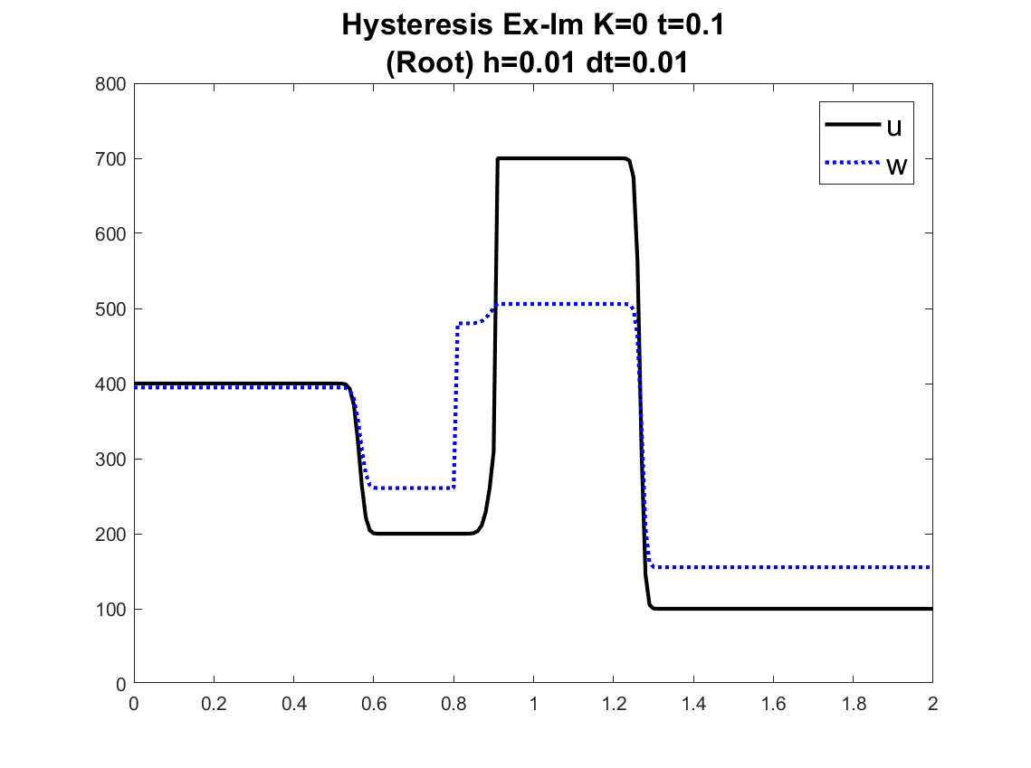
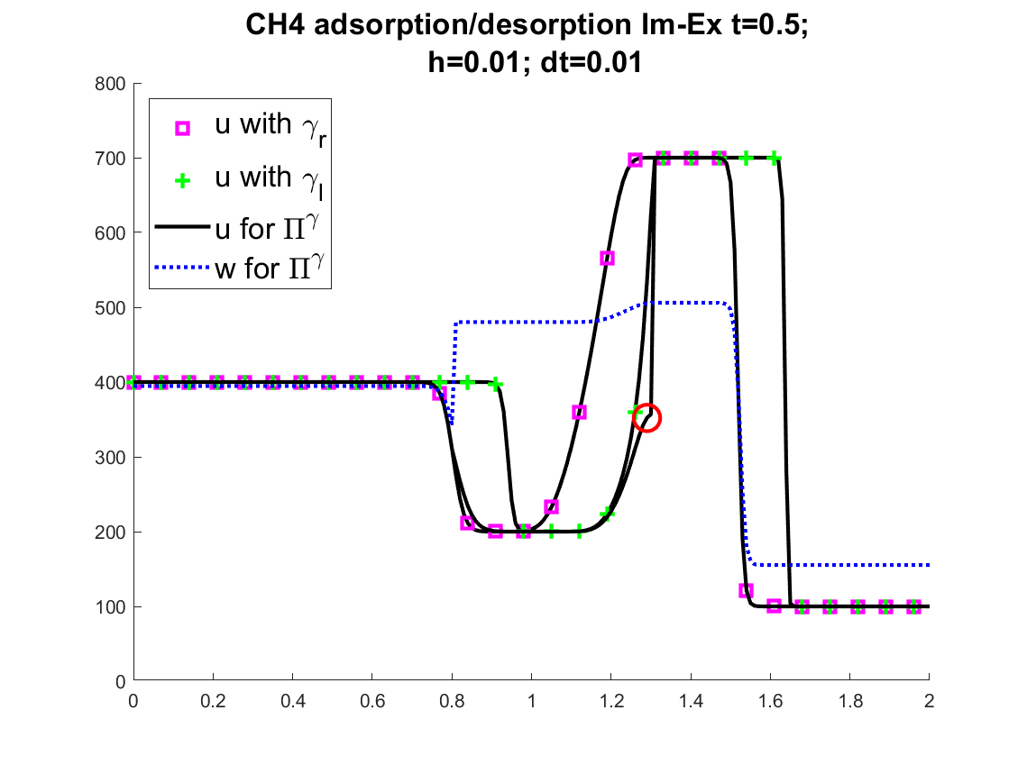
(a)	(b)
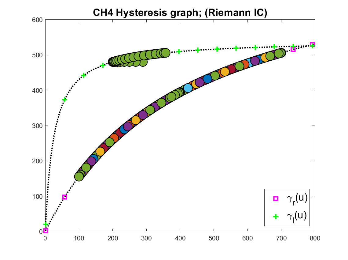
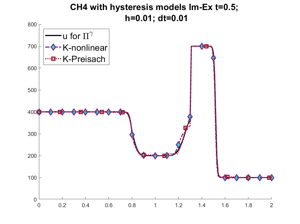
(c)	(d)

Figure 10: Illustration of transport with adsorption hysteresis models for the CH4 adsorption-desorption curves from Sec. 6.4.1. Top: (a) initial and (b) final results at $t=0.5$. Bottom: (c) the trace $(U_{j}^{n},W_{j}^{n})_{j,n}$ of $\mathcal{H}(\Pi;)$ for $\Pi=\Pi^{\gamma}$, and (d) comparison of $U_{h,\tau}(\Pi)$ for different $\Pi$.

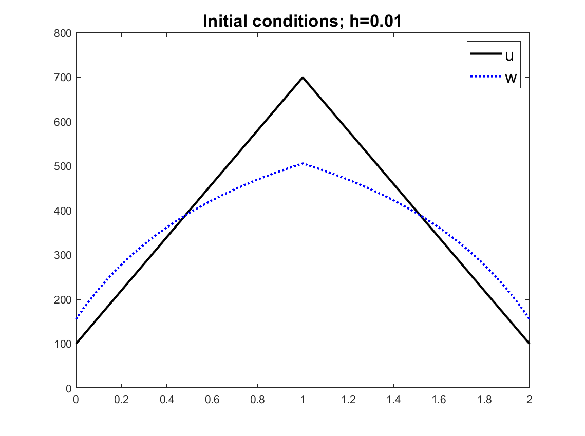
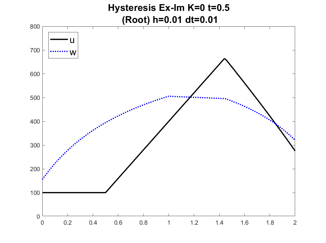
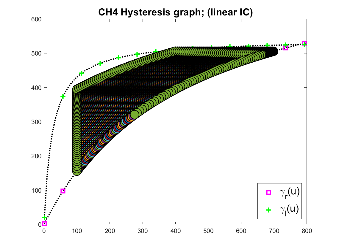
Figure 11: Simulation of transport with adsorption hysteresis from Sec. 4.6.4. Left and middle: initial and final $(U_{h,\tau},W_{h,\tau})$ with $\Pi^{\gamma}$. Right: the trace $(U_{j}^{n},W_{j}^{n})_{j,n})$ of $\mathcal{H}(\Pi^{\gamma},:)$.

6.4.2 Transport with convex-concave graph $\mathcal{H}$ from Sec. 4.6.3.

We set-up the initial condition to be the “trough” (“well”), and simulate with the different hysteresis models. We also compare the simulation with hysteresis to that without. The latter examples show the expected behavior of the sides of the “well’. If only the (convex) $\gamma_{r}$ is used, the flux function, the inverse of $u+\gamma_{r}(u)$, is concave, thus we expect a sharp front on the increasing right hand side of the well. The opposite happens when $\gamma_{l}(\cdot)$ is used.

When the hysteresis model is used with one of $\Pi^{K}_{\infty},\Pi^{K,1},\Pi^{K,\varepsilon}$, both sides of the graph show behavior typical of rarefaction which arises because of concavity of $\gamma_{r}$ on the increasing side, and the convexity of $\gamma_{l}$ on the decreasing side.

The results for all models are qualitatively consistent with this description and with each other, and the models $K$-nonlinear play, $K$-Preisach, and $K$-generalized play all give very similar resuts, with the $u(\Pi^{K,0};x,t)$ corresponding to the $K$-Preisach being the most rough. The graphs $\mathcal{H}(\Pi;\cdot)$ are very similar to each other.

The results with $K$-linear play model have the most rich secondary curves, thus the values of $u(x,t)$ corresponding to the bottom of the “well” travel with a larger variety of velocities than those for $\Pi^{K,1}$.

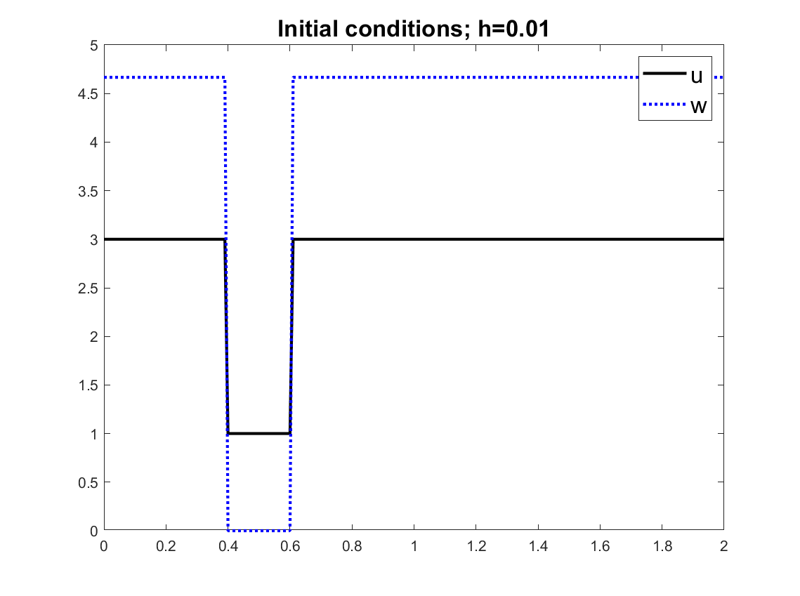
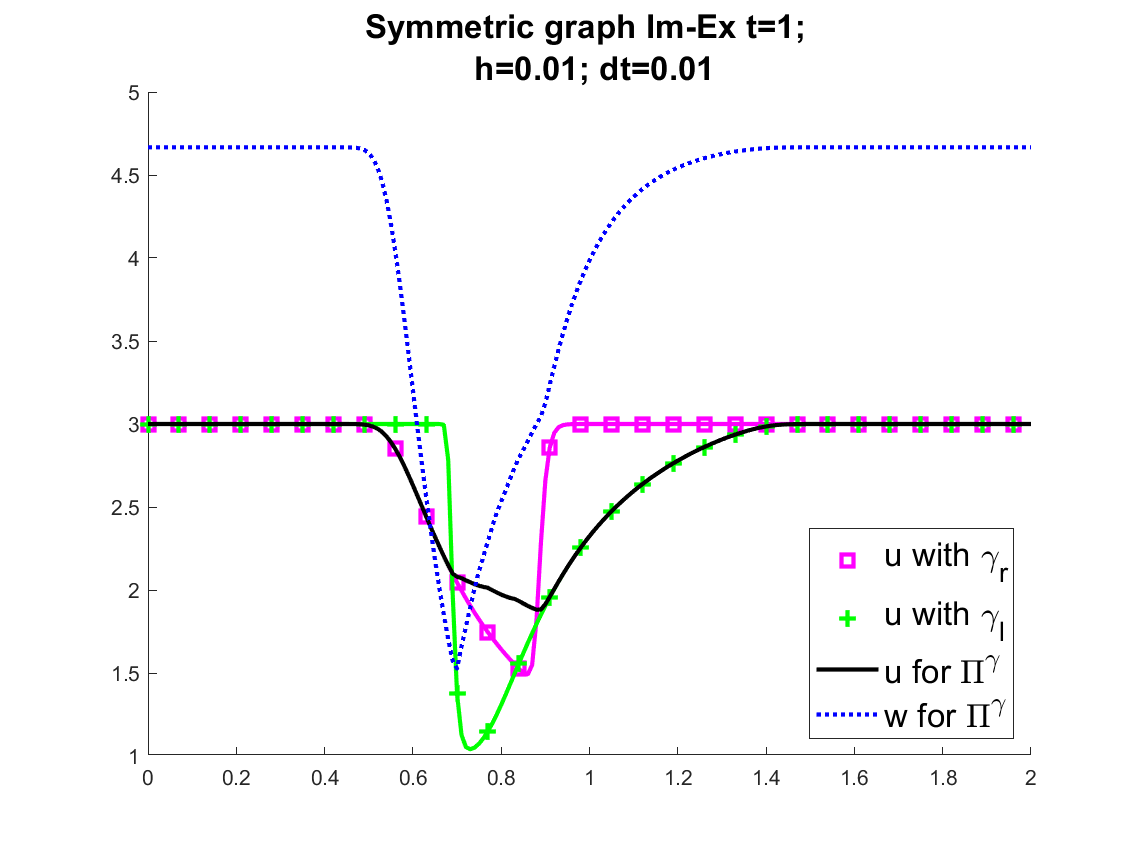
(a)	(b)
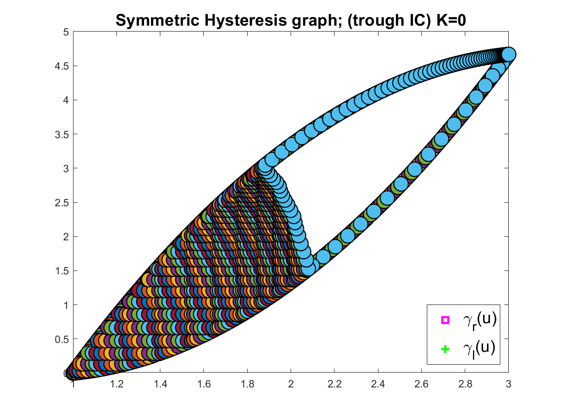
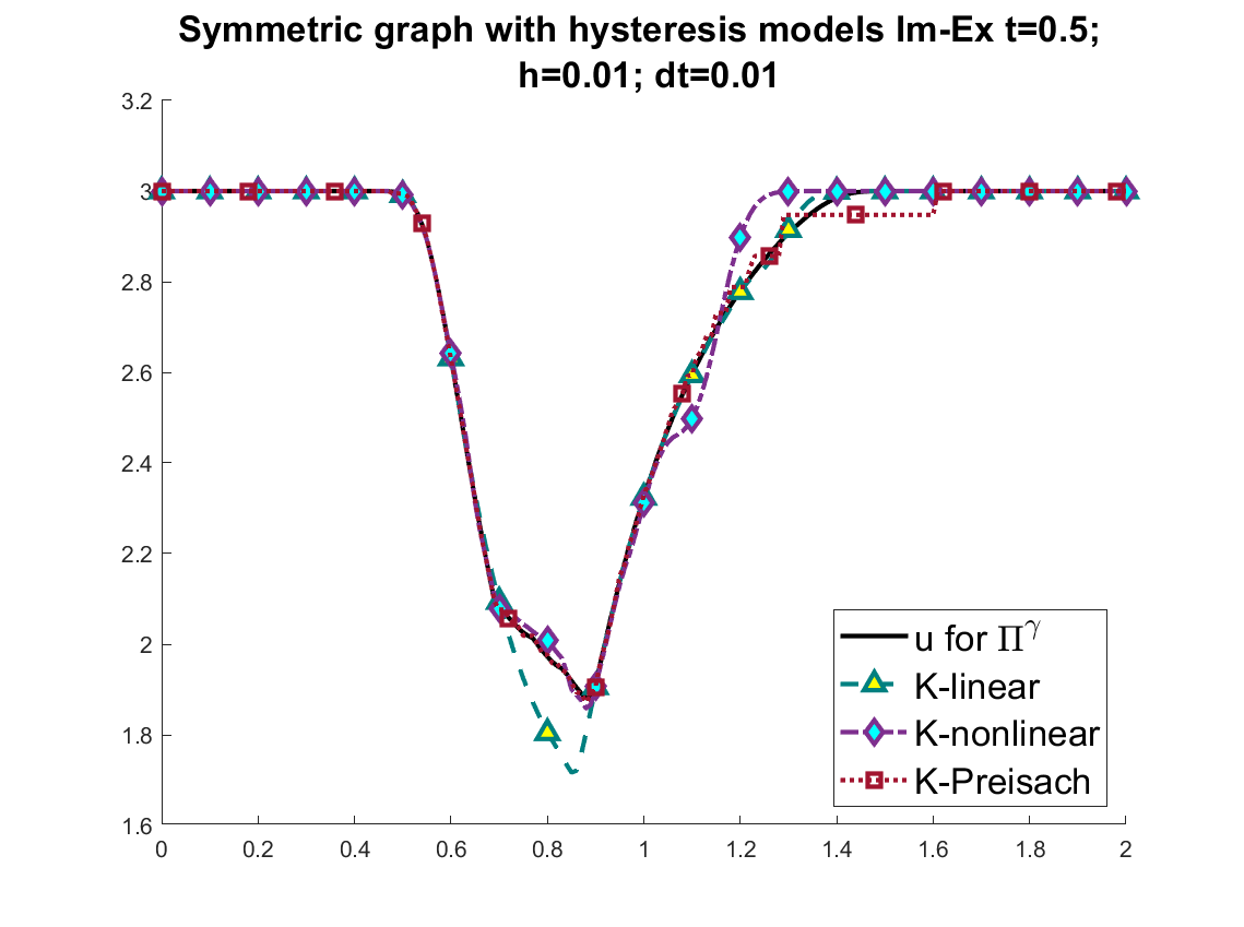
9c)	(d)
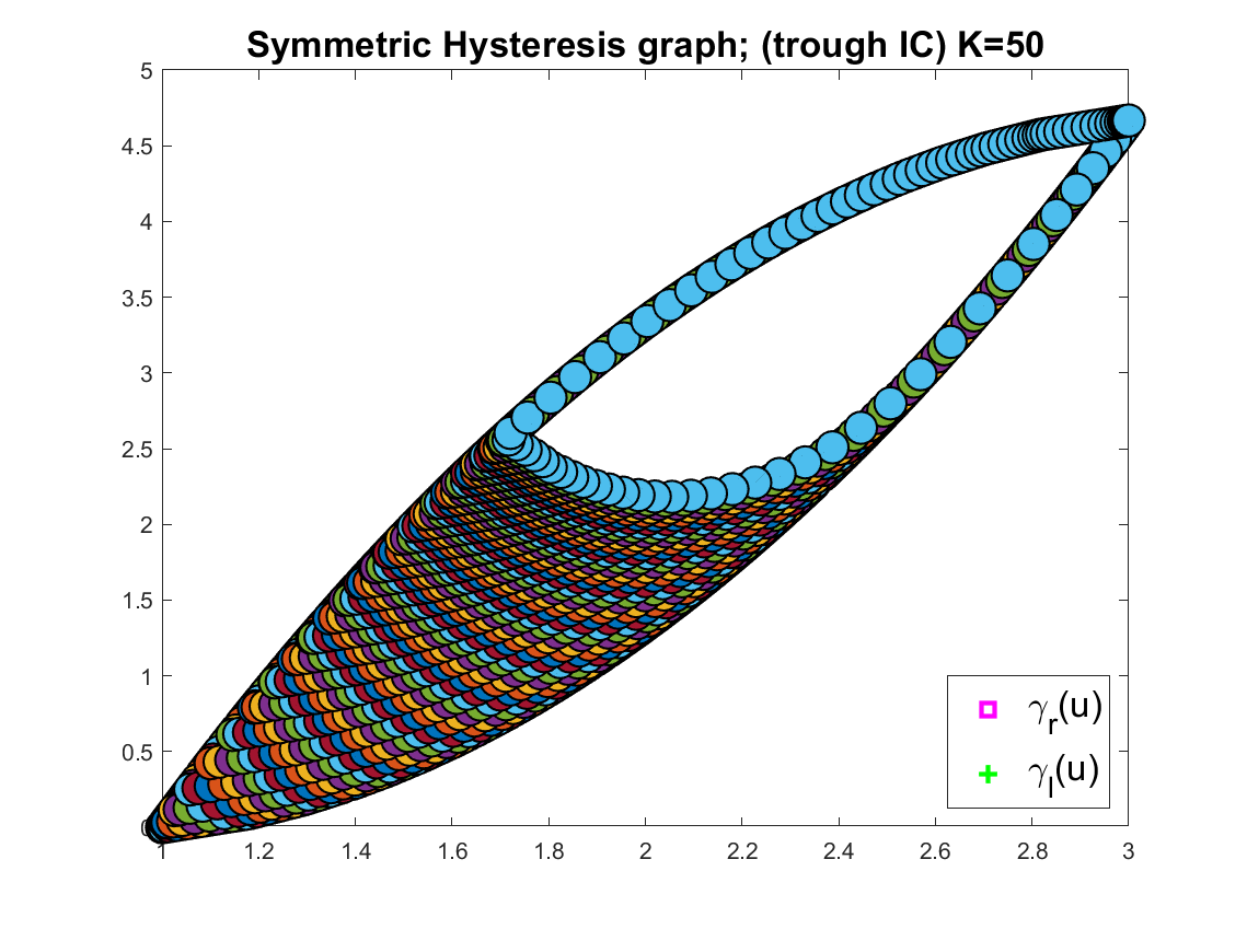
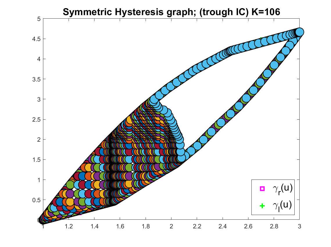
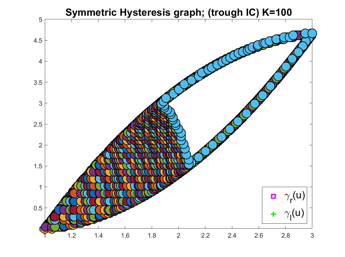
(e)ala ala ala ala ala ala (f)ala ala ala ala ala (g)

Figure 12: Simulation of adsorption hysteresis models for the graph from Sec. 4.6.4 at (a) $t=0$ and (b) $t=.5$ obtained with $\Pi^{\gamma}$. (c) Trace of $\mathcal{H}$ from $(U_{j}^{n},W_{j}^{n})_{j,n}$. (d) Results at $t=.5$ from $\Pi^{\gamma},\Pi^{K}_{\infty},\Pi^{K,1},\Pi^{K,\varepsilon}$. Bottom: the traces $\mathcal{H}(\Pi;)$ for $\Pi^{K}_{\infty},\Pi^{K,1},\Pi^{K,\varepsilon}$ with $K=50$, $K=106$, $K=100$, respectively.

6.5 Complexity of solving transport PDE with hysteresis and extensions to other temporal discretizations

It remains for us to state the cost of accounting for hysteresis when solving the transport PDE. Without hysteresis, at each time step when solving (74) we need to find $U$ from the value $a(U_{j}^{n})$ calculated explicitly from the previous the time step. This may take a few iterations of a nonlinear solver at every $j$, or require the use of a lookup table for $a^{-1}$. Generally we can say this cost is $f$ flops per each $j$ and $n$, with a rough estimate of $2<f<20$ depending on the approach taken.

With hysteresis, the cost of using $K$-nonlinear play graph depends on the number $K$ of components. Here we must find $U_{j}^{n}$, $W_{j}^{n}$ as well as all components $V_{j,k}^{n},k=1,\ldots,K$. These are found by solving the pointwise ODE (69) posed at every $j$. The resulting local nonlinear system is solved iteratively, at the following cost. In each iteration we calculate the resolvent in (69b) which is just an algebraic formula, with the cost we estimate of $\approx 5K$ per each $j$. The number of iterations is usually about two depending on the solver, thus the additional cost per each $j$ is about $\approx 10K$ per each $j$ and $n$. For the simple graph considered in Fig. 1 this amounts to about $f\approx 20$ flops, but for a complex graph such as in Fig. 6, the cost might be $f\approx 200$ when $K=42$ or $f\approx 1000$ when $K=287$ per each $j$ and $n$. The modeling precision comes with higher $K$ but also higher cost.

Refinements of the solver are possible. Clearly one can think of introducing clever refinements of time stepping and solver such as adaptivity, since not all components $k=1,\ldots,K$ are active at every point $j$ and $n$.

Lastly, we discuss the possibility of using other than fully implicit first order approaches proposed in this paper. Extensions to high order and refinements are clearly possible. However, the use of non-implicit approaches requires regularization of the component graphs which have high Lipschitz constants and require very small time-stepping for accuracy. In turn, higher order schemes are possible but may have limitations due to low temporal regularity of solutions, even away from shocks.

7 Towards calibration with secondary curves

As we discussed above, the model $K$-nonlinear play provides an easy opportunity to enhance the parametrization to account for secondary scanning curves. This is similar to the modeling power of the Preisach model. While a thorough discussion is outside our present scope, we provide a simple example to illustrate the power of $\mathcal{H}(\Pi^{K,1};\cdot)$.

Consider three parametrizations of the same primary scanning curves $H$ made of the sides of three parallelograms and shown in Fig. 13. The set $H$ can be obtained with ${\mathcal{U}}^{primary}=[0,14,0]$ so that $H=\mathcal{H}(\Pi;u)$ for $u\in\mathcal{L}({\mathcal{U}}^{primary})$

$$\Pi^{mon} = [1,1,5,1;1,3,9,1;1,7,11,1];$$ (75a)

$$\Pi^{rich} = [1,3,5,1;1,7,9,1;1,1,11,1];$$ (75b)

$$\Pi^{rich,*} = [1,3,5,b^{h}_{*};1,7,9,b^{h}_{*};1,1,11,b^{h}_{*}];h=1.$$ (75c)

with the last using the smooth truncation function (20). Next we design the input $u\in\mathcal{L}({\mathcal{U}}^{rich})$ to produce a rich variety of secondary scanning curves, and plot $\mathcal{H}(\Pi;u)$; here

$${\mathcal{U}}^{rich}=[0,14,0,6,3,5.5,3,10,7,9.5,7,11.5,3,6,3,5.5,3,10,7,9.5,7,12,7,10,7.5,10,3.5,6,3,6,1,3]$$

The results plotted in Fig. 13 show significant difference in secondary curves, without much additional computational effort.

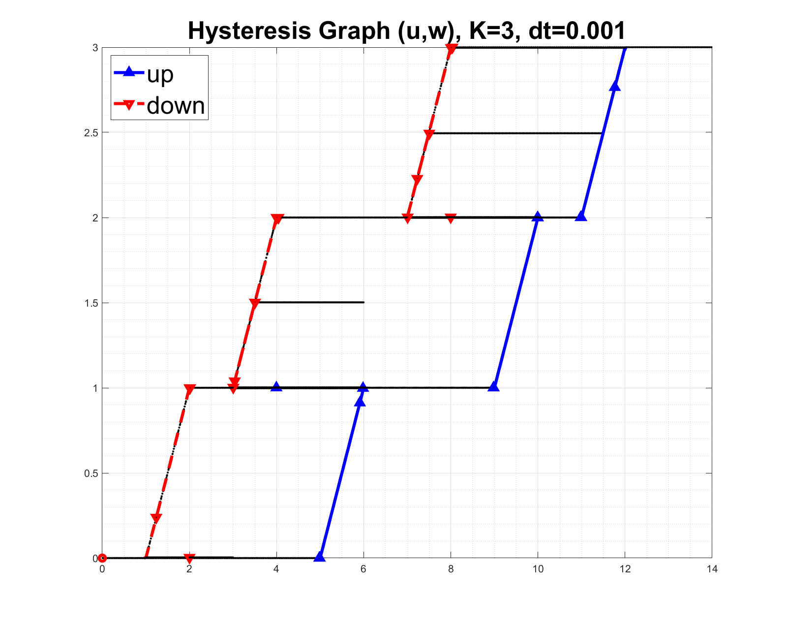
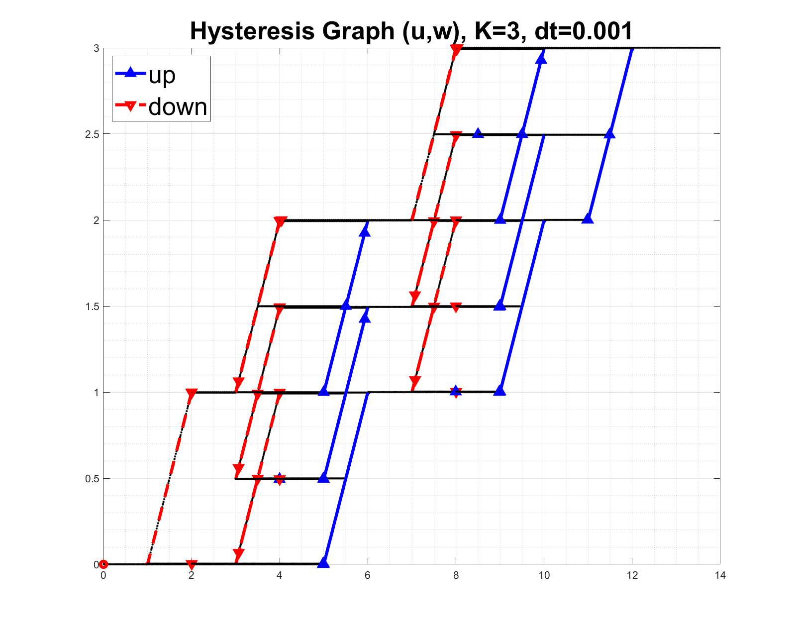
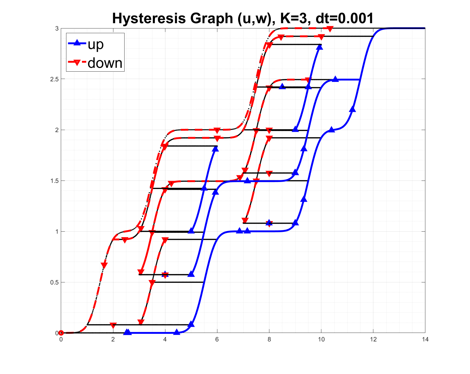
$\Pi^{mon}$	$\Pi^{rich}$	$\Pi^{rich,*}$

Figure 13: Primary and secondary scanning curves for $\Pi^{K,1}$ from (75) from Sec. 7.

$\Pi^{mon}$	$\Pi^{rich}$	$\Pi^{CH4,K},K=287$	$\Pi^{convex,K},K=100$

Figure 14: Preisach plane signatures for $\Pi^{mon}$, and $\Pi^{rich}$ from Sec. 7, as well as for $\Pi^{K,1}$ and $\Pi^{K,\varepsilon}$ found in Sec. 4.6.4 and 4.6.3. Each illustration presents the collection $(\alpha_{k},\beta_{k})_{k}$ in the upper half of the Preisach plane above the line $\beta=\alpha$. The points are colored by the measure $\mu_{k}$.

8 Summary

In this paper we presented a practical view of modeling hysteresis functionals in the case when only limited data is available. In particular, we showed how to calibrate hysteresis graphs of $K$-nonlinear play type when only the data for primary scanning curves $H$ are available. We compared the use of nonlinear play to the generalized play model, and showed that each has advantages and disadvantages, while they all share the theoretical (convergence) properties.

In particular, (i) generalized play is amenable to the same numerical and well-posedness analysis as $K$-nonlinear play. Since it uses one auxiliary equation only, it requires less computational time than $K$-nonlinear play, and no calibration. However, by design, it only features horizontal secondary scanning curves. For graphs $\mathcal{H}$ with a small gap $\gamma_{l}(u)-\gamma_{r}(u)$, this may not be significant. In addition, implementation of algorithms involving $\Pi^{\gamma}$ requires the use of functions in (14) rather than parameters as in (17), and is more disruptive to the PDE approximation code and more difficult than that of the models from $\Pi^{K,1}$ or $\Pi^{K,0}$ type.

In turn, (ii) the power and modeling potential of $K$-nonlinear play is evident from the different examples and from Sec. 7; this is not surprising since $K$-nonlinear play includes the discrete version of the Preisach model regularized with $b^{h}_{\varepsilon}$. Calibration of $K$-nonlinear play models can be done with the algorithm provided, and the efforts are not more difficult than approximation of $\gamma_{l}$ by a piecewise linear function. If $K$ is too large and modeling error not too important, one can allow small flat portions of $H^{*}\approx H$ and use the simple Preisach model $\Pi^{K,\varepsilon}$ with smaller $K$ instead.

Our current and future work involves developing further insights into convergence analysis and smoothness, as well as on algorithms for fully implicit schemes for the $K$-generalized play family and when, e.g., operator $A$ is a diffusion operator, as well as when $a(u)$ is less than strongly monotone. We are also exploring the connection between parametrization with $\Pi^{K,1}$ using secondary scanning curves, and the Preisach plane.

Appendix

8.1 Iterative algorithm for parametrization of $K$-nonlinear play

We initialize iteration by setting $\mathcal{H}_{i}^{(0)}=\mathcal{H}_{i}$; these may have curvilinear sides. In each iteration $q=1,2\ldots q^{*}$, we parametrize each $\mathcal{H}_{i}^{(q)}$

$$vert(H_{i}^{(q)})=\{(\alpha_{i}^{(q)},w_{i-1}),(\beta_{i}^{(q)},w_{i-1}),(B_{i}^{(q)},w_{i}),(A_{i}^{(q)},w_{i})\},$$ (76)

and find some $\Pi^{(q)}_{i}$ with algorithm from Sec. 4.4.1. We require continuity of the piecewise linear sides of $\mathcal{H}_{i}^{(q)}$, i.e.,

$$A^{(q)}_{i}=\alpha_{i+1}^{(q)},\;\;B^{(q)}_{i}=\beta_{i+1}^{(q)},\;\;0\leq i\leq I-1.$$ (77)

Proceeding from $q$-$1\mapsto q$ involves successive improvements of efficiency, while making sure that (77) holds. The process $q$-$1\mapsto q$ is not automatic, leaving a lot of flexibility to adapt the requirements for accuracy and efficiency to their project’s needs. For example, in this paper we choose to loop $i=1,2,\ldots I$ from “bottom” to the “top” of $\mathcal{H}$, but other strategies are possible.

Loop $q=1,\ldots q^{*}$.

Loop $i=1,\ldots I$.

Step i.A. Choose $\alpha_{i}^{(q)},\beta_{i}^{(q)}$.

If $i=1$, use $\alpha_{i}^{(q)}=\alpha_{i}^{(0)}=\alpha_{i}$, $\beta_{i}^{(q)}=\beta_{i}^{(0)}=\beta_{i}$.

If $i>1$, use $\alpha_{i}^{(q)}=A_{i-1}^{(q)}$, $\beta_{i}^{(q)}=B_{i-1}^{(q)}$. (This ensures (77)).

Step i.B. Determine $A_{i}^{(q)},B_{i}^{(q)}$ with algorithm described in Sec. 4.4.1 applied to the trial trapezoid $H_{i}^{(q-\tfrac{1}{2})}$ with the vertices

$$vert(H_{i}^{(q-\tfrac{1}{2})})=\{(\alpha_{i}^{(q)},w_{i-1}),(\alpha_{i}^{(q)},w_{i-1}),(A_{i}^{(q-\tfrac{1}{2})},w_{i}),(B_{i}^{(q-\tfrac{1}{2})},w_{i}).\}$$

Here we select $A_{i}^{(q-\tfrac{1}{2})}$ from the set $A^{(q)}=\{A_{i}^{(0)},A_{i}^{(1)},\ldots A_{i}^{(q-1)}\}$ so that the sides of $H_{i}^{(q)}$ approximate best the curves $(u,\gamma_{l}(u))$, $\alpha_{i}^{(q)}\leq u\leq\max{A^{(q)}}$. Proceed similarly for $B_{i}^{(q-\tfrac{1}{2})}$.

Next find the parametrization $\Pi_{i}^{(q)}$ and two new vertices $A_{i}^{(q)},B_{i}^{(q)}$ as in Sec. 4.4.1. Adjust these as needed for accuracy and efficiency.

Step i.C. Continue to next $i$.

End loop over $i=1,\ldots I$.

Check the quality of current approximation $\mathcal{H}^{(q)}\approx\mathcal{H}$: Assess the fit of the sides of $H_{i}^{(q)}$ to the curves $\gamma_{r}(\cdot),\gamma_{l}(\cdot)$, and whether the overall number $K=\sum_{i=1}^{I}K_{i}^{(q)}$ is small enough to be practical.

If not, set $q=q+1$ and continue to the next iteration. If yes, we’re done.

End loop over $q$. Set $q^{*}=q$, and $\mathcal{H}_{i}^{*}=\mathcal{H}_{i}^{(q)}$. Set $\Pi^{*}=(\Pi^{(q)}_{i})_{i=i}^{I}$.

References

References

- [1] A.H Al-Muhtaseb, W.A.M McMinn, and T.R.A Magee. Moisture sorption isotherm characteristics of food products: A review. Food and bioproducts processing, 80(2):118–128, 2002.
- [2] T. G. Amler, N. D. Botkin, K.-H. Hoffmann, A. M. Meirmanov, and V. N. Starovoitov. Transport equation with boundary conditions of hysteresis type. Math. Methods Appl. Sci., 32(17):2177–2196, 2009.
- [3] Robert S. Anderssen, Ivan G. Götz, and Karl-Heinz Hoffmann. The global behavior of elastoplastic and viscoelastic materials with hysteresis-type state equations. SIAM J. Appl. Math., 58(2):703–723, 1998.
- [4] Yasaman Assef, Apostolos Kantzas, and Pedro Pereira Almao. Numerical modelling of cyclic co2 injection in unconventional tight oil resources; trivial effects of heterogeneity and hysteresis in bakken formation. Fuel (Guildford), 236:1512–1528, 2019.
- [5] B Beisner, D Haydon, and K Cuddington. Hysteresis, 2008.
- [6] A Yu Beliaev and S M Hassanizadeh. A theoretical model of hysteresis and dynamic effects in the capillary relation for two-phase flow in porous media. Transport in Porous Media, 43(3):487–510, 2001.
- [7] Richard P Brent. Algorithms for minimization without derivatives, chap. 4, 1973.
- [8] H. Brézis. Opérateurs maximaux monotones et semi-groupes de contractions dans les espaces de Hilbert. North-Holland Publishing Co., Amsterdam, 1973. North-Holland Mathematics Studies, No. 5. Notas de Matemática (50).
- [9] Martin Brokate and Jürgen Sprekels. Hysteresis and phase transitions, volume 121 of Applied Mathematical Sciences. Springer-Verlag, New York, 1996.
- [10] X Cao and I.S Pop. Two-phase porous media flows with dynamic capillary effects and hysteresis: Uniqueness of weak solutions. Computers & mathematics with applications (1987), 69(7):688–695, 2015.
- [11] Katarzyna Czerw. Methane and carbon dioxide sorption/desorption on bituminous coal—experiments on cubicoid sample cut from the primal coal lump. International Journal of Coal Geology, 85(1):72–77, 2011.
- [12] Maria Fredriksson and Emil Engelund Thybring. On sorption hysteresis in wood: Separating hysteresis in cell wall water and capillary water in the full moisture range. PloS one, 14(11):e0225111, 2019.
- [13] P.A. Monson H.-J. Woo, L. Sarkisov. Understanding adsorption hysteresis in porous glasses and other mesoporous materials. In Characterization of porous solids VI ; Studies in surface science and catalysis, volume 144. 2002.
- [14] K.-H. Hoffmann and G. H. Meyer. A least squares method for finding the Preisach hysteresis operator from measurements. Numer. Math., 55(6):695–710, 1989.
- [15] K.-H. Hoffmann, J. Sprekels, and A. Visintin. Identification of hysteresis loops. J. Comput. Phys., 78(1):215–230, 1988.
- [16] Karl-Heinz Hoffmann, Nobuyuki Kenmochi, Masahiro Kubo, and Noriaki Yamazaki. Optimal control problems for models of phase-field type with hysteresis of play operator. Adv. Math. Sci. Appl., 17(1):305–336, 2007.
- [17] U. Hornung and R. E. Showalter. PDE-models with hysteresis on the boundary. In Models of hysteresis (Trento, 1991), volume 286 of Pitman Res. Notes Math. Ser., pages 30–38. Longman Sci. Tech., Harlow, 1993.
- [18] Kristian Jessen, Guo-Qing Tang, and Anthony R Kovscek. Laboratory and simulation investigation of enhanced coalbed methane recovery by gas injection. Transport in porous media, 73(2):141–159, 2007.
- [19] G. Kadar and Edward Della Torre. Determination of the bilinear product preisach function. Journal of applied physics, 63(8):3001–3003, 1988.
- [20] C. T. Kelley. Iterative methods for linear and nonlinear equations. SIAM, Philadelphia, 1995.
- [21] E. Kierlik, P. A. Monson, M. L. Rosinberg, L. Sarkisov, and G. Tarjus. Capillary condensation in disordered porous materials: Hysteresis versus equilibrium behavior. Phys. Rev. Lett., 87(5):055701, Jul 2001.
- [22] David Kinderlehrer and Guido Stampacchia. An introduction to variational inequalities and their applications, volume 88 of Pure and Applied Mathematics. Academic Press Inc. [Harcourt Brace Jovanovich Publishers], New York, 1980.
- [23] CA Kossack et al. Comparison of reservoir simulation hysteresis options. In SPE Annual Technical Conference and Exhibition. Society of Petroleum Engineers, 2000.
- [24] M. A. Krasnoselskii and A. V. Pokrovskiĭ. Systems with hysteresis. Springer-Verlag, Berlin, 1989. Translated from the Russian by Marek Niezgódka.
- [25] Pavel Krejčí. The Preisach hysteresis model: error bounds for numerical identification and inversion. Discrete Contin. Dyn. Syst. Ser. S, 6(1):101–119, 2013.
- [26] Serge Lang. Introduction to diophantine approximations. Addison-Wesley Publishing Co., Reading, Mass.-London-Don Mills, Ont., 1966.
- [27] Randall J. LeVeque. Finite volume methods for hyperbolic problems. Cambridge Texts in Applied Mathematics. Cambridge University Press, Cambridge, 2002.
- [28] B. Libby and P. A. Monson. Adsorption/desorption hysteresis in inkbottle pores: A Density Functional Theory and Monte Carlo simulation study. Langmuir, 20(10):4289–4294, 2004. PMID: 15969430.
- [29] T. D. Little and R. E. Showalter. Semilinear parabolic equations with Preisach hysteresis. Differential Integral Equations, 7(3-4):1021–1040, 1994.
- [30] Jack W. Macki, Paolo Nistri, and Pietro Zecca. Mathematical models for hysteresis. SIAM Rev., 35(1):94–123, 1993.
- [31] M. H Masud, Mohammad U. H Joardder, and M. A Karim. Effect of hysteresis phenomena of cellular plant-based food materials on convection drying kinetics. Drying technology, 37(10):1313–1320, 2018.
- [32] I. D. Mayergoyz. Mathematical models of hysteresis. Springer-Verlag, New York, 1991.
- [33] F. Patricia Medina and M. Peszynska. Hybrid modeling and analysis of multicomponent adsorption with applications to coalbed methane. In Porous Media: Theory, Properties, and Applications, isbn 978-1-63485-474-0 1, pages 1–52. Nova Science Publishers, 2016.
- [34] Alexander Mielke, Laetitia Paoli, Adrien Petrov, and Ulisse Stefanelli. Error estimates for space-time discretizations of a rate-independent variational inequality. SIAM J. Numer. Anal., 48(5):1625–1646, 2010.
- [35] Yechezkel Mualem. Modified approach to capillary hysteresis based on a similarity hypothesis. Water Resources Research, 9(5):1324–1331, 1973.
- [36] Ricardo H. Nochetto, Giuseppe Savaré, and Claudio Verdi. A posteriori error estimates for variable time-step discretizations of nonlinear evolution equations. Comm. Pure Appl. Math., 53(5):525–589, 2000.
- [37] M. Peszynska. Methane in subsurface: mathematical modeling and computational challenges. In Clint Dawson and Margot Gerritsen, editors, IMA Volumes in Mathematics and its Applications 156, Computational Challenges in the Geosciences. Springer, 2013.
- [38] M. Peszynska and R. E. Showalter. A transport model with adsorption hysteresis. Differential Integral Equations, 11(2):327–340, 1998.
- [39] Malgorzata Peszynska and Ralph E. Showalter. Approximation of scalar conservation law with hysteresis. SIAM J. Numer. Anal., 58(2):962–987, 2020.
- [40] J. R Philip. Horizontal redistribution with capillary hysteresis. Water Resources Research, 27(7):1459–1469, 1991.
- [41] Basanta Kumar Prusty. Sorption of methane and CO2 for enhanced coalbed methane recovery and carbon dioxide sequestration. Journal of Natural Gas Chemistry, 17(1):29 – 38, 2008.
- [42] Jim Rulla. Error analysis for implicit approximations to solutions to Cauchy problems. SIAM J. Numer. Anal., 33(1):68–87, 1996.
- [43] Jarl-Gunnar Salin. Inclusion of the sorption hysteresis phenomenon in future drying models: Some basic considerations. Maderas. Ciencia y tecnología, 13(2):173–182, 2011.
- [44] L. Sarkisov and P. A. Monson. Hysteresis in Monte Carlo and Molecular Dynamics simulations of adsorption in porous materials. Langmuir, 16(25):9857–9860, 2000.
- [45] Ben Schweizer. Hysteresis in porous media: Modelling and analysis. Interfaces and Free Boundaries, 19(3):417–447, 2017.
- [46] R. E. Showalter. Monotone operators in Banach space and nonlinear partial differential equations, volume 49 of Mathematical Surveys and Monographs. American Mathematical Society, Providence, RI, 1997.
- [47] Ralph E. Showalter, Thomas D. Little, and Ulrich Hornung. Parabolic PDE with hysteresis. Control Cybernet., 25(3):631–643, 1996. Distributed parameter systems: modelling and control (Warsaw, 1995).
- [48] J. C. Simo and T. J. R. Hughes. Computational inelasticity, volume 7 of Interdisciplinary Applied Mathematics. Springer-Verlag, New York, 1998.
- [49] G. C Topp. Soil‐water hysteresis: the domain theory extended to pore interaction conditions. Soil Science Society of America Journal, 35(2):219–225, 1971.
- [50] Eleuterio F. Toro. Riemann solvers and numerical methods for fluid dynamics. Springer-Verlag, Berlin, third edition, 2009. A practical introduction.
- [51] Michael Ulbrich. Semismooth Newton methods for variational inequalities and constrained optimization problems in function spaces, volume 11 of MOS-SIAM Series on Optimization. Society for Industrial and Applied Mathematics (SIAM), Philadelphia, PA, 2011.
- [52] C. Verdi and A. Visintin. Numerical approximation of hysteresis problems. IMA J. Numer. Anal., 5(4):447–463, 1985.
- [53] C. Verdi and A. Visintin. Numerical approximation of the Preisach model for hysteresis. RAIRO Modél. Math. Anal. Numér., 23(2):335–356, 1989.
- [54] A. Visintin. Hysteresis and semigroups. In Models of hysteresis (Trento, 1991), volume 286 of Pitman Res. Notes Math. Ser., pages 192–206. Longman Sci. Tech., Harlow, 1993.
- [55] Augusto Visintin. Differential models of hysteresis, volume 111 of Applied Mathematical Sciences. Springer-Verlag, Berlin, 1994.
- [56] Huangjing Zhao, Zhiping Lai, and Abbas Firoozabadi. Sorption hysteresis of light hydrocarbons and carbon dioxide in shale and kerogen. Scientific reports, 7(1):16209–10, 2017.