Securing Communications with
Friendly Unmanned Aerial Vehicle Jammers

Abstract

In this paper, we analyze the impact of a friendly unmanned aerial vehicle (UAV) jammer on UAV communications in the presence of multiple eavesdroppers. We first present channel components determined by the line-of-sight (LoS) probability between the friendly UAV jammer and the ground device, and introduce different channel fadings for LoS and non-line-of-sight (NLoS) links. We then derive the secrecy transmission probability satisfying both constraints of legitimate and wiretap channels. We also analyze the secrecy transmission probability in the presence of randomly distributed multiple friendly UAV jammers. Finally, we show the existence of the optimal UAV jammer location, and the impact of the density of eavesdroppers, the transmission power of the UAV jammer, and the density of UAV jammers on the optimal location.

I Introduction

As an UAV communication has several advantages such as the LoS environment and their flexible mobility, many researchers have studied the use of UAVs as a communication device [1]. Specifically, by using the relation between the LoS probability and the distance-dependent path loss, the optimal positioning of UAVs has been mainly studied. When the UAV height increases, the link between the UAV and the ground device forms the better link due to increasing LoS signal, while the link distance increases. Hence, several works optimized the UAV height to improve the communication performance [2, 3].

In UAV communications, the secrecy is also an important issue due to the broadcast nature of wireless channels. To overcome this, the physical layer security has recently emerged as an effective approach for communication secrecy [4, 5]. Different from terrestrial communications, in UAV communications, the UAV and the ground devices form LoS links with higher probability, so malicious eavesdroppers as well as legitimate receivers can receive the signal from the transmitting UAV with higher power. Hence, the works in [6, 7] provided the optimal deployment and trajectory of UAVs, which improve the effect of the jamming signal to the eavesdroppers, while reducing the effect of the interfering signal to the receivers. Specifically, the optimal UAV height and the transmit power were presented to minimize the secrecy outage probability in [6]. The intercept probability and the ergodic secrecy rate were presented by considering the effect of the UAV height and the transmit power in [7]. However, the works in [6, 7] did not consider the friendly jammer which can reduce the eavesdropping probability.

Recently, the friendly jammer has been considered in [8, 9, 10, 11] to improve the secrecy performance. For the case of the friendly terrestrial jammer, the optimal secrecy guard zone radius was presented to maximize secrecy throughput in [8]. Different from terrestrial communications, the UAV and the ground devices form LoS links with higher probability in UAV communications. Hence, the friendly UAV jammer can generally give stronger jamming signals to eavesdroppers than a terrestrial jammer by having LoS links to eavesdroppers. Furthermore, the friendly UAV jammer can also be readily located to maximize the jamming efficiency as it has on-demand mobility. Therefore, in recent works such as [9, 10, 11], the friendly UAV jammer has also been considered. Specifically, the secrecy energy efficiency was presented to analyze the effect of the transmission power and the density ratio of transmitters to eavesdroppers in [9]. The optimal UAV height and the secrecy guard zone size were presented to maximize the secrecy transmission capacity in [10]. The optimal deployment and transmission power of the friendly UAV jammer were provided to maximize the intercept probability security region in [11]. However, the works in [9, 10] focused on the effect of the density ratio of friendly UAV jammers to eavesdroppers instead of the specific location of the friendly UAV jammer. The optimal location of a friendly UAV jammer was presented in [11], but the channel fading for the air-to-ground (A2G) channel was not considered. In addition, the work in [11] did not show the effect of the eavesdropper density on the optimal location of the friendly UAV jammer.

In this paper, we present the effect of a friendly UAV jammer on the secrecy transmission probability. We consider channel fadings and components, affected by horizontal and vertical distances between the friendly UAV jammer and the ground devices including eavesdroppers. The main contributions of this paper can be summarized as follows:

• we consider realistic channel model, determined by the LoS probability between a friendly UAV jammer and a ground device;

• we derive the secrecy transmission probability considering different channel fadings for LoS and NLoS links;

• we also analyze the secrecy transmission probability by considering multiple UAV jammers, randomly distributed in the network; and

• we finally show the optimal location of the friendly UAV jammer that maximizes the secrecy transmission probability according to the eavesdropper density and the transmission power of the friendly UAV jammer.

II System Model

In this section, we describe the UAV network and the channel model, affected by horizontal and vertical distances between the friendly UAV jammer and ground devices.

II-A Network Description

We consider the UAV network with a transmitter (Tx), a legitimate receiver (Rx), a friendly UAV jammer (Jammer), and multiple eavesdroppers (Eves) as shown in Fig. 1. On the ground, the Tx and the Rx are located at $\boldsymbol{q}_{\text{t}}=(0,0,0)$ and $\boldsymbol{q}_{\text{r}}=(x_{\text{r}},y_{\text{r}},0)$, respectively. Eves are randomly distributed by a Poisson point process (PPP) $\Phi_{\text{e}}\triangleq\{\boldsymbol{q}_{\text{e}_{i}}\}$ with density $\lambda_{\text{e}}$, where $\boldsymbol{q}_{\text{e}_{i}}=(x_{\text{e}_{i}},y_{\text{e}_{i}},0)$ is the location of an arbitrary Eve [12]. Each Eve decodes the received signal from the Tx independently, i.e., we consider non-colluding Eves. The Jammer is placed in an adjustable location $\boldsymbol{q}_{\text{u}}=(x_{\text{u}},y_{\text{u}},z_{\text{u}})$. In this network, we assume the Tx and the Jammer do not know the locations of Eves. We also assume the legitimate channel (between Tx and Rx in the presence of Jammer) and the wiretap channel (between Tx and Eves in the presence of Jammer) are independent.

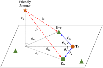
Figure 1: System model where multiple eavesdroppers are randomly distributed on the ground and a friendly UAV jammer is in the air. The blue lines represent transmitting signals from the transmitter and the red dotted lines represent interfering signals from the friendly UAV jammer.

Based on $\boldsymbol{q}_{\text{t}}$, $\boldsymbol{q}_{\text{r}}$, $\boldsymbol{q}_{\text{e}_{i}}$, and $\boldsymbol{q}_{\text{u}}$, we define the signal-to-interference-plus-noise ratio (SINR) of the legitimate channel $(c=\text{r})$ or the wiretap channel $(c=\text{e}_{i})$ as

$$\gamma_{c} =\frac{h_{\text{t}c}\ell_{c}^{-\alpha_{\text{t}c}}P_{\text{t}}}{h_{\text{u}c}j_{c}(d_{c},z_{\text{u}})^{-\alpha_{\text{u}c}}P_{\text{u}}+\sigma^{2}}$$

$$=\frac{h_{\text{t}c}\rho_{c}}{h_{\text{u}c}\tau_{c}(d_{c},z_{\text{u}})+\sigma^{2}},\quad\quad c\in\{\text{r},\text{e}_{i}\}$$ (1)

where $\ell_{c}=\sqrt{x_{c}^{2}+y_{c}^{2}}$ is the link distance between the Tx and the Rx $(c=\text{r})$ or the Eve $(c=\text{e}_{i})$, $j_{c}(d_{c},z_{\text{u}})=\sqrt{(x_{\text{u}}-x_{c})^{2}+(y_{\text{u}}-y_{c})^{2}+z_{\text{u}}^{2}}$ is the link distance between the Jammer and the Rx $(c=\text{r})$ or the Eve $(c=\text{e}_{i})$, $P_{\text{t}}$ and $P_{\text{u}}$ are the transmission power of the Tx and the Jammer, respectively, and $\sigma^{2}$ is the noise power. Here, $h_{\text{t}c}$ and $h_{\text{u}c}$ are channel fading gains, and $\alpha_{\text{t}c}$ and $\alpha_{\text{u}c}$ are path loss exponents, where the subscript $\text{t}c$ represents the transmission from the Tx to the Rx $(c=\text{r})$ or the Eve $(c=\text{e}_{i})$, and the subscript $\text{u}c$ represents the transmission from the Jammer to the Rx $(c=\text{r})$ or the Eve $(c=\text{e}_{i})$. In (1), for convenience, we introduce $\rho_{c}=\ell_{c}^{-\alpha_{\text{t}c}}P_{\text{t}}$ and $\tau_{c}(d_{c},z_{\text{u}})=j_{c}(d_{c},z_{\text{u}})^{-\alpha_{\text{u}c}}P_{\text{u}}$, where $d_{c}=\sqrt{(x_{\text{u}}-x_{c})^{2}+(y_{\text{u}}-y_{c})^{2}}$ is horizontal distance between the Jammer and the Rx $(c=\text{r})$ or the Eve $(c=\text{e}_{i})$, which can be expressed as

$$d_{c}=\sqrt{d_{\text{tu}}^{2}+\ell_{c}^{2}-2d_{\text{tu}}\ell_{c}\cos{\theta_{c}}}$$ (2)

where $d_{\text{tu}}$ is the horizontal distance between the Jammer and the Tx, and $\theta_{c}$ is the included angle between $\ell_{c}$ and $d_{\text{tu}}$ as shown in Fig. 1.

II-B Channel Model

Since all the devices except for the Jammer are located on the ground, there can be two types of channels, which are the ground-to-ground (G2G) channel and the A2G channel. The G2G channel between ground devices is commonly modeled as the NLoS environment with the Rayleigh fading due to a lot of obstacles. On the other hand, the A2G channel between the Jammer and the ground device (e.g., the interference link to Rx and the jamming link to Eve) can have the LoS or NLoS environment according to the existence of obstacles. In this subsection, we introduce channel components and provide the model of the A2G channel.

II-B1 Channel component

On UAV communications, channel components such as the LoS probability and the path loss exponent are affected by the horizontal distance $d_{c}$ and the vertical distance $z_{\text{u}}$ between a Jammer and a Rx $(c=\text{r})$ or a Eve $(c=\text{e}_{i})$. First, when the heights of ground devices are sufficiently small, the LoS probability, $p_{\text{L}}(d_{c},z_{\text{u}})$, $c\in\{\text{r},\text{e}_{i}\}$, is given by [14]

$$p_{\text{L}}(d_{c},z_{\text{u}})=\left\{1-\frac{\sqrt{2\pi}\zeta}{z_{\text{u}}}\Bigg{|}Q\left(\frac{z_{\text{u}}}{\zeta}\right)-0.5\Bigg{|}\right\}^{d_{c}\sqrt{\nu\mu}}$$ (3)

where $Q(x)=\int_{x}^{\infty}\frac{1}{\sqrt{2\pi}}\exp\left(-\frac{t^{2}}{2}\right)\,dt$ is the Q-function, and $\zeta$, $\nu$, and $\mu$ are environment parameters, determined by the building density and height. We then define the NLoS probability as $p_{\text{N}}(d_{c},z_{\text{u}})=1-p_{\text{L}}(d_{c},z_{\text{u}})$. Note that the LoS probability can be applicable in various environments (e.g., urban, suburban, and dense urban) by adjusting the environment parameters. In addition, the path loss exponent $\alpha_{\text{u}c}$ is determined by $\alpha_{\text{L}}$ when the A2G channel is in the LoS environment. Otherwise, $\alpha_{\text{u}c}=\alpha_{\text{N}}$.

II-B2 Air-to-Ground (A2G) channel

In the A2G channel, as the received signal power at the ground device is affected by the combination of the LoS and NLoS signals [16], we consider that the channel fading is the Nakagami-$m$ fading with mean $\overline{H_{\text{L}}}=1$ for the LoS environment and the Rayleigh fading with mean $\overline{H_{\text{N}}}=1$ for the NLoS environment. Therefore, the distribution of channel fading gains, $h_{\text{u}c}$, $c\in\{\text{r},\text{e}_{i}\}$, can be expressed as

$$f_{h_{\text{u}c}}^{(\text{L})}(h) =\frac{m_{\text{L}}^{m_{\text{L}}}h^{m_{\text{L}}-1}}{\Gamma\left(m_{\text{L}}\right)}\exp\left(-m_{\text{L}}h\right)\quad\text{for \acs{LoS}}$$

$$f_{h_{\text{u}c}}^{(\text{N})}(h) =\exp\left(-h\right)\quad\quad\quad\quad\quad\,\,\,\quad\quad\text{for \acs{NLoS}}$$ (4)

where $m_{\text{L}}$ is the Nakagami-$m$ fading parameter and $\Gamma(z)=\int_{0}^{\infty}x^{z-1}e^{-x}dx$ is the gamma function.

III Secrecy Transmission Probability Analysis

In this section, for given $d_{\text{r}}$ and $z_{\text{u}}$, we analyze the secrecy transmission probability $p_{\text{se}}(d_{\text{r}},z_{\text{u}})$, which is the probability that a Tx reliably transmits signals to a Rx, while all the Eves fail to eavesdrop, and is defined as [8]

$$p_{\text{se}}(d_{\text{r}},z_{\text{u}}) =\mathbb{P}\left[\gamma_{\text{r}}>\gamma_{\text{t}},\max\limits_{\text{e}_{i}\in\Phi_{\text{e}}}\gamma_{\text{e}_{i}}<\gamma_{\text{t}}^{\prime}\right]$$ (5)

where $\gamma_{\text{t}}$ and $\gamma_{\text{t}}^{\prime}$ are target SINRs of the legitimate channel and the wiretap channel, respectively.

Lemma 1

The secrecy transmission probability can be presented as

$$p_{\text{se}}(d_{\text{r}},z_{\text{u}})=p_{\text{s}}(d_{\text{r}},z_{\text{u}})(1-p_{\text{e}}(z_{\text{u}}))$$ (6)

where $p_{\text{s}}(d_{\text{r}},z_{\text{u}})$ and $p_{\text{e}}(z_{\text{u}})$ are given by

$$p_{\text{s}}(d_{\text{r}},z_{\text{u}})=\frac{m_{\text{L}}^{m_{\text{L}}}}{\left(\frac{\gamma_{\text{t}}\tau_{\text{r}}(d_{\text{r}},z_{\text{u}})}{\rho_{\text{r}}}+m_{\text{L}}\right)^{m_{\text{L}}}}\exp\left(-\frac{\gamma_{\text{t}}\sigma^{2}}{\rho_{\text{r}}}\right)p_{\text{L}}(d_{\text{r}},z_{\text{u}})$$

$$\quad\quad\quad\quad\,\,\,+\frac{\rho_{\text{r}}}{\rho_{\text{r}}+\gamma_{\text{t}}\tau_{\text{r}}(d_{\text{r}},z_{\text{u}})}\exp\left(-\frac{\gamma_{\text{t}}\sigma^{2}}{\rho_{\text{r}}}\right)p_{\text{N}}(d_{\text{r}},z_{\text{u}}),$$ (7)

$$p_{\text{e}}(z_{\text{u}})=1-\exp\left\{-\lambda_{\text{e}}\int_{0}^{2\pi}\int_{0}^{\infty}p_{\text{s,e}_{i}}(\ell_{\text{e}_{i}},\theta_{\text{e}_{i}},z_{\text{u}})\ell_{\text{e}_{i}}d\ell_{\text{e}_{i}}d\theta_{\text{e}_{i}}\right\}.$$ (8)

In (8), $p_{\text{s,e}_{i}}(\ell_{\text{e}_{i}},\theta_{\text{e}_{i}},z_{\text{u}})=\mathbb{P}\left[\gamma_{\text{e}_{i}}>\gamma_{\text{t}}^{\prime}\right]$, which is presented from (7) by substituting from $d_{\text{r}}$, $\rho_{\text{r}}$, and $\gamma_{\text{t}}$ to $d_{\text{e}_{i}}$, $\rho_{\text{e}_{i}}$, and $\gamma_{\text{t}}^{\prime}$, respectively.

Proof:

For given $\boldsymbol{q}_{\text{t}}$, $\boldsymbol{q}_{\text{u}}$, $\boldsymbol{q}_{\text{e}_{i}}$, and $\boldsymbol{q}_{\text{r}}$, we can obtain the secrecy transmission probability $p_{\text{se}}(d_{\text{r}},z_{\text{u}})$ as

$$p_{\text{se}}(d_{\text{r}},z_{\text{u}}) =\mathbb{P}\left[\gamma_{\text{r}}>\gamma_{\text{t}},\max\limits_{\text{e}_{i}\in\Phi_{\text{e}}}\gamma_{\text{e}_{i}}<\gamma_{\text{t}}^{\prime}\right]$$

$$\overset{\underset{\mathrm{(a)}}{}}{=}p_{\text{s}}(d_{\text{r}},z_{\text{u}})(1-p_{\text{e}}(z_{\text{u}}))$$ (9)

where $p_{\text{s}}(d_{\text{r}},z_{\text{u}})=\mathbb{P}\left[\gamma_{\text{r}}>\gamma_{\text{t}}\right]$ is the successful transmission probability, $p_{\text{e}}(z_{\text{u}})=\mathbb{P}\left[\max\limits_{\text{e}_{i}\in\Phi_{\text{e}}}\gamma_{\text{e}_{i}}>\gamma_{\text{t}}^{\prime}\right]$ is the eavesdropping probability, and (a) is obtained due to the independence between the legitimate channel and the wiretap channel. In (9), $p_{\text{s}}(d_{\text{r}},z_{\text{u}})$ can be obtained as [2]

$$p_{\text{s}}(d_{\text{r}},z_{\text{u}})=\int_{0}^{\infty}\int_{\frac{\gamma_{\text{t}}\left(\tau_{\text{r}}(d_{\text{r}},z_{\text{u}})g+\sigma^{2}\right)}{\rho_{\text{r}}}}^{\infty}f_{h_{\text{tr}}}(h)dhf_{h_{\text{ur}}}(g)dg$$

$$=p_{\text{s}}^{(\text{L})}(d_{\text{r}},z_{\text{u}})p_{\text{L}}(d_{\text{r}},z_{\text{u}})+p_{\text{s}}^{(\text{N})}(d_{\text{r}},z_{\text{u}})p_{\text{N}}(d_{\text{r}},z_{\text{u}})$$ (10)

where $p_{\text{s}}^{(e_{\text{I}})}(d_{\text{r}},z_{\text{u}})$ is the successful transmission probability in the environment of the interference link $e_{\text{I}}$, given by

$$p_{\text{s}}^{(\text{L})}(d_{\text{r}},z_{\text{u}})=\int_{0}^{\infty}\int_{\frac{\gamma_{\text{t}}\left(\tau_{\text{r}}(d_{\text{r}},z_{\text{u}})g+\sigma^{2}\right)}{\rho_{\text{r}}}}^{\infty}f_{h_{\text{tr}}}(h)\,dhf_{h_{\text{ur}}}^{(\text{L})}(g)\,dg$$

$$\overset{\underset{\mathrm{(a)}}{}}{=}\int_{0}^{\infty}\exp\left\{-\frac{\gamma_{\text{t}}\left(\tau_{\text{r}}(d_{\text{r}},z_{\text{u}})g+\sigma^{2}\right)}{\rho_{\text{r}}}-m_{\text{L}}g\right\}\frac{m_{\text{L}}^{m_{\text{L}}}g^{m_{\text{L}}-1}}{\Gamma(m_{\text{L}})}dg,$$ (11)

$$p_{\text{s}}^{(\text{N})}(d_{\text{r}},z_{\text{u}})=\int_{0}^{\infty}\int_{\frac{\gamma_{\text{t}}\left(\tau_{\text{r}}(d_{\text{r}},z_{\text{u}})g+\sigma^{2}\right)}{\rho_{\text{r}}}}^{\infty}f_{h_{\text{tr}}}(h)\,dhf_{h_{\text{ur}}}^{(\text{N})}(g)\,dg$$

$$\overset{\underset{\mathrm{(a)}}{}}{=}\int_{0}^{\infty}\exp\left\{-\frac{\gamma_{\text{t}}\left(\tau_{\text{r}}(d_{\text{r}},z_{\text{u}})g+\sigma^{2}\right)}{\rho_{\text{r}}}-g\right\}dg.$$ (12)

Here, (a) is from the cumulative distribution function (CDF) of the exponential distribution. In (11), by [17, eq. (3.326)], the integral term can be expressed as

$$\int_{0}^{\infty}x^{m}\exp\left(-\beta x^{n}\right)dx=\frac{\Gamma(\gamma)}{n\beta^{\gamma}}$$ (13)

where $m=m_{\text{L}}-1$, $n=1$, $\beta=\frac{\gamma_{\text{t}}\tau_{\text{r}}(d_{\text{r}},z_{\text{u}})}{\rho_{\text{r}}}+m_{\text{L}}$, and $\gamma=\frac{m+1}{n}$. By using (13) in (11) and the definite integral in (12), $p_{\text{s}}(d_{\text{r}},z_{\text{u}})$ is presented as (7).

In the wiretap channel, $p_{\text{e}}(z_{\text{u}})$ can be derived as

$$p_{\text{e}}(z_{\text{u}})=\mathbb{P}\left[\max\limits_{\text{e}_{i}\in\Phi_{\text{e}}}\gamma_{\text{e}_{i}}>\gamma_{\text{t}}^{\prime}\right]=1-\mathbb{E}_{\Phi_{\text{e}}}\left[\prod_{\text{e}_{i}\in\Phi_{\text{e}}}\mathbb{P}\left[\gamma_{\text{e}_{i}}<\gamma_{\text{t}}^{\prime}\right]\right].$$ (14)

By using the probability generating functional (PGFL) in (14), $p_{\text{e}}(z_{\text{u}})$ is presented as (8). ∎

From Lemma 1, we can know that $p_{\text{s}}(d_{\text{r}},z_{\text{u}})$ and $p_{\text{e}}(z_{\text{u}})$ decrease with $m_{\text{L}}$. Using this result, the impact of $m_{\text{L}}$ on $p_{\text{se}}(d_{\text{r}},z_{\text{u}})$ is shown and discussed in the numerical results.

Corollary 1

For given $z_{\text{u}}$, $\ell_{r}$, and $d_{\text{tu}}$, the optimal value of $\theta_{\text{r}}$ that maximizes $p_{\text{se}}(d_{\text{tu}},z_{\text{u}},\theta_{\text{r}})$ is $\pi$.

Proof:

For convenience, we introduce $F(d_{\text{tu}},z_{\text{u}})=\int_{0}^{2\pi}\int_{0}^{\infty}p_{\text{s,e}_{i}}(\ell_{\text{e}_{i}},\theta_{\text{e}_{i}},z_{\text{u}})\ell_{\text{e}_{i}}d\ell_{\text{e}_{i}}d\theta_{\text{e}_{i}}$ and represent $p_{\text{se}}(d_{\text{r}},z_{\text{u}})$ as functions of $d_{\text{tu}}$, $z_{\text{u}}$, and $\theta_{\text{r}}$ as

$$p_{\text{se}}(d_{\text{tu}},z_{\text{u}},\theta_{\text{r}})=p_{\text{s}}(d_{\text{tu}},z_{\text{u}},\theta_{\text{r}})\exp\left\{-\lambda_{\text{e}}F(d_{\text{tu}},z_{\text{u}})\right\}.$$ (15)

In (15), for given $z_{\text{u}}$, $\ell_{r}$, and $d_{\text{tu}}$, we obtain the first derivative of $p_{\text{se}}(d_{\text{tu}},z_{\text{u}},\theta_{\text{r}})$ with respect to $\theta_{\text{r}}$ as

$$\frac{\partial p_{\text{se}}(d_{\text{tu}},z_{\text{u}},\theta_{\text{r}})}{\partial\theta_{\text{r}}}=\exp\left\{-\lambda_{\text{e}}F(d_{\text{tu}},z_{\text{u}})\right\}\left\{\frac{\partial p_{\text{L}}(d_{\text{tu}},z_{\text{u}},\theta_{\text{r}})}{\partial\theta_{\text{r}}}\right.$$

$$\left.\times\left(p_{\text{s}}^{(\text{L})}(d_{\text{tu}},z_{\text{u}},\theta_{\text{r}})-p_{\text{s}}^{(\text{N})}(d_{\text{tu}},z_{\text{u}},\theta_{\text{r}})\right)+\frac{\partial p_{\text{s}}^{(\text{L})}(d_{\text{tu}},z_{\text{u}},\theta_{\text{r}})}{\partial\theta_{\text{r}}}\right.$$

$$\left.\times p_{\text{L}}(d_{\text{tu}},z_{\text{u}},\theta_{\text{r}})+\frac{\partial p_{\text{s}}^{(\text{N})}(d_{\text{tu}},z_{\text{u}},\theta_{\text{r}})}{\partial\theta_{\text{r}}}p_{\text{N}}(d_{\text{tu}},z_{\text{u}},\theta_{\text{r}})\right\}.$$ (16)

In (16), for $z_{\text{u}}>0$, $p_{\text{s}}^{(\text{L})}(d_{\text{tu}},z_{\text{u}},\theta_{\text{r}})-p_{\text{s}}^{(\text{N})}(d_{\text{tu}},z_{\text{u}},\theta_{\text{r}})<0$, $p_{\text{L}}(d_{\text{tu}},z_{\text{u}},\theta_{\text{r}})>0$, and $p_{\text{N}}(d_{\text{tu}},z_{\text{u}},\theta_{\text{r}})>0$. In addition, from (3), we obtain $\frac{\partial p_{\text{L}}(d_{\text{tu}},z_{\text{u}},\theta_{\text{r}})}{\partial\theta_{\text{r}}}=-C_{1}\sin(\theta_{\text{r}})$, $\frac{\partial p_{\text{s}}^{(\text{L})}(d_{\text{tu}},z_{\text{u}},\theta_{\text{r}})}{\partial\theta_{\text{r}}}=C_{2}\sin(\theta_{\text{r}})$, and $\frac{\partial p_{\text{s}}^{(\text{N})}(d_{\text{tu}},z_{\text{u}},\theta_{\text{r}})}{\partial\theta_{\text{r}}}=C_{3}\sin(\theta_{\text{r}})$ for positive $C_{1}$, $C_{2}$, and $C_{3}$. Hence, the stationary values of $\theta_{\text{r}}$ are obtained when $\sin(\theta_{\text{r}})=0$. Furthermore, we readily know that $p_{\text{s}}(d_{\text{tu}},z_{\text{u}},\pi)$ is greater than $p_{\text{s}}(d_{\text{tu}},z_{\text{u}},0)$ because $p_{\text{L}}(d_{\text{tu}},z_{\text{u}},\pi)$ is smaller than $p_{\text{L}}(d_{\text{tu}},z_{\text{u}},0)$ and $\tau_{\text{r}}(d_{\text{tu}},z_{\text{u}},\pi)$ is smaller than $\tau_{\text{r}}(d_{\text{tu}},z_{\text{u}},0)$. Therefore, the optimal value of $\theta_{\text{r}}$ that maximizes $p_{\text{se}}(d_{\text{tu}},z_{\text{u}},\theta_{\text{r}})$ is $\pi$. ∎

From Corollary 1, we can see that the Jammer needs to be located along the line from the Rx to the Tx. Hence, in Section V, we analyze $p_{\text{se}}(d_{\text{tu}},z_{\text{u}},\pi)$ instead of $p_{\text{se}}(d_{\text{tu}},z_{\text{u}},\theta_{\text{r}})$.

We now present the asymptotic secrecy transmission probability when the Jammer is located near to the Tx.

Corollary 2

As the Jammer approaches to the Tx, the asymptotic secrecy transmission probability can be given by

$$p_{\text{se}}(d_{\text{r}},z_{\text{u}})\approx p_{\text{s}}(d_{\text{r}},z_{\text{u}})\exp\left\{\frac{-2\lambda_{\text{e}}\pi P_{\text{t}}\Gamma\left(\frac{2}{\alpha_{\text{N}}}\right)}{\left(\gamma_{\text{t}}^{\prime}P_{\text{u}}+P_{\text{t}}\right)\alpha_{\text{N}}\left(\frac{\gamma_{\text{t}}^{\prime}\sigma^{2}}{P_{\text{t}}}\right)^{\frac{2}{\alpha_{\text{N}}}}}\right\}$$ (17)

where $p_{\text{s}}(d_{\text{r}},z_{\text{u}})$ is given in (7).

Proof:

In (8), as $d_{\text{tu}}\rightarrow 0$ (i.e., when the Jammer approaches to the Tx with the height $z_{\text{u}}$), the eavesdropping probability $p_{\text{e}}(z_{\text{u}})$ can be given by

$$p_{\text{e}}(z_{\text{u}}) \approx 1-\exp\left[-2\pi\lambda_{\text{e}}\int_{0}^{\infty}\left\{\exp\left(-\frac{\gamma_{\text{t}}^{\prime}\sigma^{2}}{\rho_{\text{e}_{i}}}\right)\right.\right.$$

$$\left.\left.\quad\times\frac{m_{\text{L}}^{m_{\text{L}}}p_{\text{L}}(\ell_{\text{e}_{i}},z_{\text{u}})}{\left(\frac{\gamma_{\text{t}}^{\prime}P_{\text{u}}\left(\ell_{\text{e}_{i}}^{2}+z_{\text{u}}^{2}\right)^{-\frac{\alpha_{\text{L}}}{2}}}{\rho_{\text{e}_{i}}}+m_{\text{L}}\right)^{m_{\text{L}}}}+\exp\left(-\frac{\gamma_{\text{t}}^{\prime}\sigma^{2}}{\rho_{\text{e}_{i}}}\right)\right.\right.$$

$$\left.\left.\quad\times\frac{\rho_{\text{e}_{i}}p_{\text{N}}(\ell_{\text{e}_{i}},z_{\text{u}})}{\rho_{\text{e}_{i}}+\gamma_{\text{t}}^{\prime}P_{\text{u}}\left(\ell_{\text{e}_{i}}^{2}+z_{\text{u}}^{2}\right)^{-\frac{\alpha_{\text{N}}}{2}}}\right\}\ell_{\text{e}_{i}}d\ell_{\text{e}_{i}}\right].$$ (18)

In (18), when $z_{\text{u}}$ is small, $p_{\text{L}}(\ell_{\text{e}_{i}},z_{\text{u}})$ approaches to zero and $p_{\text{e}}(z_{\text{u}})$ can be represented as

$$p_{\text{e}}\approx 1-\exp\left\{-2\pi\lambda_{\text{e}}\int_{0}^{\infty}\frac{P_{\text{t}}}{P_{\text{t}}+\gamma_{\text{t}}^{\prime}P_{\text{u}}}\exp\left(-\frac{\gamma_{\text{t}}^{\prime}\sigma^{2}}{P_{\text{t}}\ell_{\text{e}_{i}}^{-\alpha_{\text{N}}}}\right)\ell_{\text{e}_{i}}d\ell_{\text{e}_{i}}\right\}.$$ (19)

Using the following result [17, eq. (3.326)]

$$\int_{0}^{\infty}x^{m}\exp\left(-\beta x^{n}\right)dx=\frac{\Gamma(\gamma)}{n\beta^{\gamma}}$$ (20)

with $m=1$, $n=\alpha_{\text{N}}$, $\beta=\frac{\gamma_{\text{t}}^{\prime}\sigma^{2}}{P_{t}}$, and $\gamma=\frac{m+1}{n}$, $p_{\text{e}}$ in (19) can be presented in a closed-form. Finally, we can obtain the asymptotic expression of $p_{\text{se}}(d_{\text{r}},z_{\text{u}})$ as (17). ∎

From Corollary 2, we can readily see the effect of the network parameters (e.g., main link distance and transmission power of Tx) on the secrecy transmission probability.

IV Secrecy Transmission Probability Analysis With Multiple UAV Jammers

In this section, we now consider multiple UAV jammers, which are randomly distributed by a PPP $\Phi_{\text{u}}$ with density $\lambda_{\text{u}}$ at the height $z_{\text{u}}$. The channel components and fading gains between the typical Jammer and the ground device are the same as the single Jammer case. From the secrecy transmission probability in (6), we obtain the secrecy transmission probability for multiple UAV jammers in the following corollary.

Corollary 3

In the presence of multiple UAV jammers, the secrecy transmission probability $\tilde{p}_{\text{se}}(z_{\text{u}})$ is given by

$$\tilde{p}_{\text{se}}(z_{\text{u}})=\exp\left\{-2\pi\lambda_{\text{u}}\int_{0}^{\infty}\left(1-\sum_{e_{\text{I}}\in\{\text{L},\text{N}\}}\hat{p}_{\text{s}}^{(e_{\text{I}})}(r,z_{\text{u}})p_{e_{\text{I}}}(r,z_{\text{u}})\right)rdr\right.$$

$$\left.-\frac{\gamma_{\text{t}}\sigma^{2}}{\rho_{\text{r}}}\right\}\exp\left[-2\pi\lambda_{\text{e}}\int_{0}^{\infty}\exp\left\{-\frac{\gamma_{\text{t}}^{\prime}\sigma^{2}}{\rho_{\text{e}_{i}}}-2\pi\lambda_{\text{u}}\right.\right.$$

$$\left.\left.\times\int_{0}^{\infty}\left(1-\sum_{e_{\text{J}}\in\{\text{L},\text{N}\}}\hat{p}_{\text{s,e}_{i}}^{(e_{\text{J}})}(v,z_{\text{u}})p_{e_{\text{J}}}(v,z_{\text{u}})\right)vdv\right\}\ell_{\text{e}_{i}}d\ell_{\text{e}_{i}}\right]$$ (21)

where $\hat{p}_{\text{s}}^{(e_{\text{I}})}(r,z_{\text{u}})$ is the successful transmission probability of the interference limited environment (i.e., $\sigma^{2}=0$ in (11) and (12)) and $r$ is the horizontal distance between the Jammer and the Rx. In (21), $\hat{p}_{\text{s,e}_{i}}^{(e_{\text{J}})}(v,z_{\text{u}})$ is obtained from $\hat{p}_{\text{s}}^{(e_{\text{I}})}(r,z_{\text{u}})$ by replacing $d_{\text{u}_{i}\text{r}}$, $\rho_{\text{r}}$, and $\gamma_{\text{t}}$ with $d_{\text{u}_{i}{\text{e}_{i}}}$, $\rho_{\text{e}_{i}}$, and $\gamma_{\text{t}}^{\prime}$, respectively. Here, $e_{\text{J}}$ is the environment of the jamming link and $v$ is the horizontal distance between the Jammer and the Eve.

Proof:

For given $z_{\text{u}}$, the secrecy transmission probability for multiple UAV jammers can be presented as

$$\tilde{p}_{\text{se}}(z_{\text{u}})=\mathbb{E}_{\Phi_{\text{u}}}\left[\mathbb{P}\left[\frac{h_{\text{tr}}\rho_{\text{r}}}{\sum_{\text{u}_{i}\in\Phi_{\text{u}}}h_{\text{u}_{i}\text{r}}\tau_{\text{r}}(d_{\text{u}_{i}\text{r}},z_{\text{u}})+\sigma^{2}}>\gamma_{\text{t}}\right]\right]$$

$$\quad\times\mathbb{E}_{\Phi_{\text{u}}}\left[\mathbb{P}\left[\max\limits_{\text{e}_{i}\in\Phi_{\text{e}}}\frac{h_{\text{te}_{i}}\rho_{\text{e}_{i}}}{\sum_{\text{u}_{i}\in\Phi_{\text{u}}}h_{\text{u}_{i}\text{e}_{i}}\tau_{\text{e}_{i}}(d_{\text{u}_{i}{\text{e}_{i}}},z_{\text{u}})+\sigma^{2}}<\gamma_{\text{t}}^{\prime}\right]\right]$$

$$\overset{\underset{\mathrm{(a)}}{}}{=}\mathbb{E}_{\Phi_{\text{u}}}\left[\prod_{\text{u}_{i}\in\Phi_{\text{u}}}\mathbb{E}_{h_{\text{u}_{i}\text{r}}}\left[\exp\left(-\frac{\gamma_{\text{t}}h_{\text{u}_{i}\text{r}}\tau_{\text{r}}(d_{\text{u}_{i}\text{r}},z_{\text{u}})}{\rho_{\text{r}}}\right)\right]\right]$$

$$\quad\times\exp\left(-\frac{\gamma_{\text{t}}\sigma^{2}}{\rho_{\text{r}}}\right)\mathbb{E}_{\Phi_{\text{e}}}\left[\prod_{\text{e}_{i}\in\Phi_{\text{e}}}\left\{1-\exp\left(-\frac{\gamma_{\text{t}}^{\prime}\sigma^{2}}{\rho_{\text{e}_{i}}}\right)\right.\right.$$

$$\quad\left.\left.\times\mathbb{E}_{\Phi_{\text{u}}}\left[\prod_{\text{u}_{i}\in\Phi_{\text{u}}}\mathbb{E}_{h_{\text{u}_{i}{\text{e}_{i}}}}\left[\exp\left(-\frac{\gamma_{\text{t}}^{\prime}h_{\text{u}_{i}{\text{e}_{i}}}\tau_{\text{e}_{i}}(d_{\text{u}_{i}{\text{e}_{i}}},z_{\text{u}})}{\rho_{\text{e}_{i}}}\right)\right]\right]\right\}\right]$$

$$\overset{\underset{\mathrm{(b)}}{}}{=}\mathbb{E}_{\Phi_{\text{u}}}\left[\prod_{\text{u}_{i}\in\Phi_{\text{u}}}\sum_{e_{\text{I}}\in\{\text{L},\text{N}\}}\hat{p}_{\text{s}}^{(e_{\text{I}})}(d_{\text{u}_{i}\text{r}},z_{\text{u}})p_{e_{\text{I}}}(d_{\text{u}_{i}\text{r}},z_{\text{u}})\right]\exp\left(-\frac{\gamma_{\text{t}}\sigma^{2}}{\rho_{\text{r}}}\right)$$

$$\quad\times\mathbb{E}_{\Phi_{\text{e}}}\left[\prod_{\text{e}_{i}\in\Phi_{\text{e}}}\left\{1-\exp\left(-\frac{\gamma_{\text{t}}^{\prime}\sigma^{2}}{\rho_{\text{e}_{i}}}\right)\right.\right.$$

$$\quad\left.\left.\times\mathbb{E}_{\Phi_{\text{u}}}\left[\prod_{\text{u}_{i}\in\Phi_{\text{u}}}\sum_{e_{\text{J}}\in\{\text{L},\text{N}\}}\hat{p}_{\text{s,e}_{i}}^{(e_{\text{J}})}(d_{\text{u}_{i}\text{e}_{i}},z_{\text{u}})p_{e_{\text{J}}}(d_{\text{u}_{i}\text{e}_{i}},z_{\text{u}})\right]\right\}\right]$$ (22)

where (a) is obtained because $h_{\text{tr}}\sim\exp(1)$ and $h_{\text{te}_{i}}\sim\exp(1)$, and (b) is from the CDF of $h_{\text{u}_{i}{\text{r}}}$ and $h_{\text{u}_{i}{\text{e}_{i}}}$. By using the PGFL in (22), $\tilde{p}_{\text{se}}(z_{\text{u}})$ is presented as (21). ∎

In a similar way to the Corollary 2, we provide the asymptotic analysis of the secrecy transmission probability for multiple UAV jammers. Specifically, in (21), when $z_{\text{u}}$ goes zero, $p_{\text{L}}(r,z_{\text{u}})$ and $p_{\text{L}}(v,z_{\text{u}})$ approach to zero and the secrecy transmission probability can be represented as

$$\tilde{p}_{\text{se}} \approx\exp\left\{-2\pi\lambda_{\text{u}}\int_{0}^{\infty}\frac{\gamma_{\text{t}}P_{\text{u}}\ell_{\text{r}}^{\alpha_{\text{N}}}r}{P_{\text{t}}r^{\alpha_{\text{N}}}+\gamma_{\text{t}}P_{\text{u}}\ell_{\text{r}}^{\alpha_{\text{N}}}}\,dr-\frac{\gamma_{\text{t}}\sigma^{2}}{P_{\text{t}}\ell_{\text{r}}^{-\alpha_{\text{N}}}}\right\}$$

$$\quad\times\exp\left[-2\pi\lambda_{\text{e}}\int_{0}^{\infty}\exp\left\{-\frac{\gamma_{\text{t}}^{\prime}\sigma^{2}\ell_{\text{e}_{i}}^{\alpha_{\text{N}}}}{P_{\text{t}}}\right.\right.$$

$$\left.\left.\quad-2\pi\lambda_{\text{u}}\int_{0}^{\infty}\frac{\gamma_{\text{t}}^{\prime}P_{\text{u}}\ell_{\text{e}_{i}}^{\alpha_{\text{N}}}v}{P_{\text{t}}v^{\alpha_{\text{N}}}+\gamma_{\text{t}}^{\prime}P_{\text{u}}\ell_{\text{e}_{i}}^{\alpha_{\text{N}}}}\,dv\right\}\ell_{\text{e}_{i}}d\ell_{\text{e}_{i}}\right].$$ (23)

where the integral term is represented as [17, eq. (3.241)]

$$\int_{0}^{\infty}\frac{x^{\mu-1}}{\left(p+qx^{\nu}\right)^{n+1}}dx=\frac{1}{\nu p^{n+1}}\left(\frac{p}{q}\right)^{\frac{\mu}{\nu}}\frac{\Gamma\left(\frac{\mu}{\nu}\right)\Gamma\left(1+n-\frac{\mu}{\nu}\right)}{\Gamma\left(1+n\right)}$$ (24)

with $p=\gamma_{\text{t}}P_{\text{u}}\ell_{\text{r}}^{\alpha_{\text{N}}}$ (or $p=\gamma_{\text{t}}^{\prime}P_{\text{u}}\ell_{\text{e}_{i}}^{\alpha_{\text{N}}}$), $q=P_{\text{t}}$, $\nu=\alpha_{\text{N}}$, $\mu=2$, and $n=0$. By using (24) in (23) and $\Gamma(x)\Gamma(1-x)=\frac{\pi}{\sin(\pi x)}$, $\tilde{p}_{\text{se}}$ can be expressed as

$$\tilde{p}_{\text{se}} \approx\exp\left\{-\frac{2\pi^{2}\lambda_{\text{u}}}{\alpha_{\text{N}}\sin\left(\frac{2\pi}{\alpha_{\text{N}}}\right)}\left(\frac{\gamma_{\text{t}}\ell_{\text{r}}^{\alpha_{\text{N}}}P_{\text{u}}}{P_{\text{t}}}\right)^{\frac{2}{\alpha_{\text{N}}}}-\frac{\gamma_{\text{t}}\sigma^{2}}{P_{\text{t}}\ell_{\text{r}}^{-\alpha_{\text{N}}}}\right\}$$

$$\quad\times\exp\left[-2\pi\lambda_{\text{e}}\int_{0}^{\infty}\exp\left\{-\frac{\gamma_{\text{t}}^{\prime}\sigma^{2}\ell_{\text{e}_{i}}^{\alpha_{\text{N}}}}{P_{\text{t}}}\right.\right.$$

$$\quad\left.\left.-\frac{2\pi^{2}\lambda_{\text{u}}}{\alpha_{\text{N}}\sin\left(\frac{2\pi}{\alpha_{\text{N}}}\right)}\left(\frac{\gamma_{\text{t}}^{\prime}P_{\text{u}}}{P_{\text{t}}}\right)^{\frac{2}{\alpha_{\text{N}}}}\ell_{\text{e}_{i}}^{2}\right\}\ell_{\text{e}_{i}}d\ell_{\text{e}_{i}}\right].$$ (25)

In (25), when $\alpha_{\text{N}}=4$, by substituting $\ell_{\text{e}_{i}}^{2}=t$, $\tilde{p}_{\text{se}}$ is given by

$$\tilde{p}_{\text{se}} \approx\exp\left\{-\frac{\pi^{2}\lambda_{\text{u}}}{2}\left(\frac{\gamma_{\text{t}}\ell_{\text{r}}^{4}P_{\text{u}}}{P_{\text{t}}}\right)^{\frac{1}{2}}-\frac{\gamma_{\text{t}}\sigma^{2}}{P_{\text{t}}\ell_{\text{r}}^{-4}}\right\}\exp\left[-\pi\lambda_{\text{e}}\int_{0}^{\infty}\right.$$

$$\left.\quad\times\exp\left\{-\frac{\gamma_{\text{t}}^{\prime}\sigma^{2}t^{2}}{P_{\text{t}}}-\frac{\pi^{2}\lambda_{\text{u}}}{2}\left(\frac{\gamma_{\text{t}}^{\prime}P_{\text{u}}}{P_{\text{t}}}\right)^{\frac{1}{2}}t\right\}\,dt\right].$$ (26)

Using the following result [17, eq. (3.322)]

$$\int_{0}^{\infty}\exp\left(-\frac{x^{2}}{4\beta}-\gamma x\right)dx=\sqrt{\pi\beta}\exp\left(\beta\gamma^{2}\right)\left\{1-\Phi\left(\gamma\sqrt{\beta}\right)\right\}$$ (27)

with $\beta=\frac{P_{\text{t}}}{4\gamma_{\text{t}}^{\prime}\sigma^{2}}$ and $\gamma=\frac{\pi^{2}\lambda_{\text{u}}}{2}\left(\frac{\gamma_{\text{t}}^{\prime}P_{\text{u}}}{P_{\text{t}}}\right)^{\frac{1}{2}}$, $\tilde{p}_{\text{se}}$ in (26) can be presented in closed-form as

$$\tilde{p}_{\text{se}} \approx\exp\left[-\frac{\pi^{2}\lambda_{\text{u}}\left(\frac{\gamma_{\text{t}}\ell_{\text{r}}^{4}P_{\text{u}}}{P_{\text{t}}}\right)^{\frac{1}{2}}}{2}-\frac{\gamma_{\text{t}}\sigma^{2}}{P_{\text{t}}\ell_{\text{r}}^{-4}}-\pi\lambda_{\text{e}}\sqrt{\frac{\pi P_{\text{t}}}{4\gamma_{\text{t}}^{\prime}\sigma^{2}}}\right.$$

$$\left.\quad\times\exp\left(\frac{\pi^{4}\lambda_{\text{u}}^{2}P_{\text{u}}}{16\sigma^{2}}\right)\left\{1-\Phi\left(\frac{\pi^{2}\lambda_{\text{u}}}{4}\sqrt{\frac{P_{\text{u}}}{\sigma^{2}}}\right)\right\}\right]$$ (28)

where $\Phi\left(x\right)=\frac{2}{\sqrt{\pi}}\int_{0}^{\pi}\exp\left(-t^{2}\right)dt$ is the error function. From this result, we can see the effect of $\lambda_{\text{u}}$ on the secrecy transmission probability.

V Numerical Results

In this section, we evaluate the secrecy transmission probability depending on the location and the transmission power of the Jammer. Unless otherwise specified, the values of simulation parameters are $\alpha_{\text{N}}=3.5$, $\alpha_{\text{L}}=2.5$, $m_{\text{L}}=2$, $\nu=5\times 10^{-4}$, $\mu=0.3$, $\zeta=15$, $R=10000m$, $\gamma_{\text{t}}=3$, $\gamma_{\text{t}}^{\prime}=2.5$, $P_{\text{t}}=10^{-8}W$, $P_{\text{u}}=3\times 10^{-10}W$, and $\sigma^{2}=3\times 10^{-19}W$.

\psfrag{AAAAAAAAAAAAAAAAA1111}[Bl][Bl][0.59]{$z_{\text{u}}=0m$ (Ground Jammer)}\psfrag{B1}[Bl][Bl][0.59]{$z_{\text{u}}=100m$}\psfrag{C1}[Bl][Bl][0.59]{$z_{\text{u}}=200m$}\psfrag{D1}[Bl][Bl][0.59]{Simulation}\psfrag{E1}[Bl][Bl][0.59]{$\lambda_{\text{e}}=5\times 10^{-7}[\text{nodes/}m^{2}]$}\psfrag{F1}[Bl][Bl][0.59]{$\lambda_{\text{e}}=7\times 10^{-7}[\text{nodes/}m^{2}]$}\psfrag{G1}[Bl][Bl][0.59]{Asymptotic analysis}\psfrag{H1}[Bl][Bl][0.59]{$m_{\text{L}}=2$}\psfrag{J1}[Bl][Bl][0.59]{$m_{\text{L}}=9$}\psfrag{X1}[Bl][Bl][0.75]{Horizontal distance between Tx and Jammer, $d_{\text{tu}}\>[m]$}\psfrag{Y1}[Bl][Bl][0.75]{Secrecy Transmission Probability, $p_{\text{se}}(d_{\text{tu}},z_{\text{u}},\pi)$}\includegraphics[width=195.12767pt]{Figure1.eps}

Figure 2: Secrecy transmission probabilities $p_{\text{se}}(d_{\text{tu}},z_{\text{u}},\pi)$ as a function of $d_{\text{tu}}$ with $\ell_{\text{r}}=340m$ for different values of $\lambda_{\text{e}}$ and $z_{\text{u}}$. The optimal values of $d_{\text{tu}}$ are marked by circles.

Figure 2 presents the secrecy transmission probability $p_{\text{se}}(d_{\text{tu}},z_{\text{u}},\pi)$ as a function of the horizontal distance between the Jammer and the Tx $d_{\text{tu}}$ with $\ell_{\text{r}}=340m$ for different values of the Eve density $\lambda_{\text{e}}$ and the Jammer height $z_{\text{u}}$. From Fig. 2, we can see that $p_{\text{se}}(d_{\text{tu}},z_{\text{u}},\pi)$ first increases with $d_{\text{tu}}$ up to a certain value of $d_{\text{tu}}$, and then decreases. This is because for small $d_{\text{tu}}$, the decrease in the LoS probability of the interference link to the receiver is greater than that of the jamming link to the Eve with $\max\limits_{\text{e}_{i}\in\Phi_{\text{e}}}\gamma_{\text{e}_{i}}$, who mainly affects the eavesdropping probability. On the other hand, for large $d_{\text{tu}}$, as $d_{\text{tu}}$ increases, the Eve with $\max\limits_{\text{e}_{i}\in\Phi_{\text{e}}}\gamma_{\text{e}_{i}}$ can be located closer to the Tx than the Rx, so $p_{\text{se}}(d_{\text{tu}},z_{\text{u}},\pi)$ decreases with $d_{\text{tu}}$. We can also see that as $\lambda_{\text{e}}$ increases, the optimal value of $d_{\text{tu}}$ decreases to make the jamming link stronger as there exist more Eves. From this, we can find out that as the density of Eves increases, the Jammer needs to be located nearer to the Tx. In Fig. 2, we can additionally see the impact of $m_{\text{L}}$ on $p_{\text{se}}(d_{\text{r}},z_{\text{u}})$ according to $d_{\text{tu}}$. Specifically, for small $d_{\text{tu}}$, $p_{\text{se}}(d_{\text{r}},z_{\text{u}})$ decreases with $m_{\text{L}}$ since $p_{\text{s}}(d_{\text{r}},z_{\text{u}})$ decreases with $m_{\text{L}}$ more than $p_{\text{e}}(z_{\text{u}})$. On the other hand, for large $d_{\text{tu}}$, $p_{\text{se}}(d_{\text{r}},z_{\text{u}})$ increases with $m_{\text{L}}$ since $p_{\text{s}}(d_{\text{r}},z_{\text{u}})$ becomes similar for different $m_{\text{L}}$, but $p_{\text{e}}(z_{\text{u}})$ still decreases with $m_{\text{L}}$. Hence, the optimal value of $d_{\text{tu}}$ increases with $m_{\text{L}}$, which means the Jammer needs to be located further from the Tx as $m_{\text{L}}$ increases. Furthermore, we can know that the asymptotic analysis almost matches the analytic analysis as the Jammer approaches to the Tx (i.e., as $d_{\text{tu}}\rightarrow 0$ for $z_{\text{u}}=0$).

\psfrag{AAAAAAAAAAAAAAAAAAA11}[Bl][Bl][0.59]{$\lambda_{\text{e}}=1.2\times 10^{-8}[\text{nodes/}m^{2}]$}\psfrag{B}[Bl][Bl][0.59]{$\lambda_{\text{e}}=7\times 10^{-8}[\text{nodes/}m^{2}]$}\psfrag{C}[Bl][Bl][0.59]{$\lambda_{\text{e}}=3.5\times 10^{-7}[\text{nodes/}m^{2}]$}\psfrag{D}[Bl][Bl][0.59]{$\lambda_{\text{e}}=7.5\times 10^{-7}[\text{nodes/}m^{2}]$}\psfrag{E}[Bl][Bl][0.59]{$\lambda_{\text{e}}=9.3\times 10^{-7}[\text{nodes/}m^{2}]$}\psfrag{X}[Bl][Bl][0.75]{Height of Jammer, $z_{\text{u}}\>[m]$}\psfrag{Y}[Bl][Bl][0.75]{Horizontal distance between Tx and Jammer, $d_{\text{tu}}\>[m]$}\includegraphics[width=195.12767pt]{Figure2.eps}

Figure 3: Secrecy transmission probability $p_{\text{se}}(d_{\text{tu}},z_{\text{u}},\pi)$ as functions of $z_{\text{u}}$ and $d_{\text{tu}}$ with $\lambda_{\text{e}}=7.5\times 10^{-7}[\text{nodes/}m^{2}]$ and $\ell_{\text{r}}=420m$. The optimal Jammer locations for each $\lambda_{\text{e}}$ that maximize $p_{\text{se}}(d_{\text{tu}},z_{\text{u}},\pi)$ are marked by symbols.

Figure 3 presents the secrecy transmission probability $p_{\text{se}}(d_{\text{tu}},z_{\text{u}},\pi)$ as functions of the Jammer height $z_{\text{u}}$ and the horizontal distance between the Tx and the Jammer $d_{\text{tu}}$ with $\ell_{\text{r}}=420m$. The symbols mean the optimal Jammer locations, $z_{\text{u}}^{*}$ and $d_{\text{tu}}^{*}$, for each Eve density $\lambda_{\text{e}}$. From Fig. 3, we can see that $d_{\text{tu}}^{*}$ first decrease with $\lambda_{\text{e}}$ up to a certain value of $\lambda_{\text{e}}$, and then increase. This is because, for small $\lambda_{\text{e}}$ (e.g., $\lambda_{\text{e}}\leq 7\times 10^{-8}\text{nodes/}m^{2}$), since there exist less eavesdroppers, the Jammer needs to be located at the low height to reduce the LoS probability of interference link to the Rx. However, for relatively high $\lambda_{\text{e}}$ (e.g., $\lambda_{\text{e}}=3.5\times 10^{-7}\text{nodes/}m^{2}$), the Jammer needs to be located closer to the Tx, especially by reducing the horizontal distance $d_{\text{tu}}$ for giving stronger jamming signal to Eves, although it also gives larger interference to the Rx. Additionally, when $\lambda_{\text{e}}$ is much higher (e.g., $\lambda_{\text{e}}\geq 7.5\times 10^{-7}\text{nodes/}m^{2}$), since there exist many Eves, the Jammer needs to give much stronger jamming signal to Eves. Hence, the Jammer is located at the high height to increase the LoS probability of the jamming link.

\psfrag{AAAAAAAAAAAAAAAAAA11}[Bl][Bl][0.59]{$\lambda_{\text{u}}=7\times 10^{-6}[\text{nodes/}m^{2}]$}\psfrag{B1}[Bl][Bl][0.59]{$\lambda_{\text{u}}=9\times 10^{-6}[\text{nodes/}m^{2}]$}\psfrag{C1}[Bl][Bl][0.59]{$P_{\text{u}}=2\times 10^{-11}W$}\psfrag{D1}[Bl][Bl][0.59]{$P_{\text{u}}=3\times 10^{-11}W$}\psfrag{X1}[Bl][Bl][0.75]{Height of UAV jammers, $z_{\text{u}}\>[m]$}\psfrag{Y1}[Bl][Bl][0.75]{$\tilde{p}_{\text{se}}(z_{\text{u}})$}\includegraphics[width=195.12767pt]{Figure3.eps}

Figure 4: Secrecy transmission probability $\tilde{p}_{\text{se}}(z_{\text{u}})$ as a function of $z_{\text{u}}$ for different values of $\lambda_{\text{u}}$ and $P_{\text{u}}$. The optimal values of $z_{\text{u}}$ are marked by circles.

Figure 4 presents the secrecy transmission probability $\tilde{p}_{\text{se}}(z_{\text{u}})$ as a function of the height of UAV jammers $z_{\text{u}}$ for different values of the UAV jammer density $\lambda_{\text{u}}$ and the transmission power of the UAV jammer. Here, we use $\ell_{\text{r}}=50m$ and $\lambda_{\text{e}}=10^{-5}\text{nodes/}m^{2}$. From Fig. 4, we can see that $\tilde{p}_{\text{se}}(z_{\text{u}})$ first increases with $z_{\text{u}}$ up to a certain value of $z_{\text{u}}$, and then decreases. This is because for small $z_{\text{u}}$, the increase in the LoS probability of the jamming link is greater than that of the interference link. On the other hand, for large $z_{\text{u}}$, the LoS probability of the interference link keeps increasing, while the distance-dependent path loss of the eavesdropping link decreases. Therefore, $\tilde{p}_{\text{se}}(z_{\text{u}})$ decreases with $z_{\text{u}}$ when large $z_{\text{u}}$. We can also see that as $\lambda_{\text{u}}$ increases, the optimal value of $z_{\text{u}}$ decreases to give weaker LoS probability (i.e., weaker signal) on the interference link to the Rx. Furthermore, the optimal value of $z_{\text{u}}$ increases as $P_{\text{u}}$ increases. From these results, we can know that when the effect of UAV jammers is strong enough by using the larger transmit power, the UAV jammers need to be located at the low height to reduce the LoS probability of the interfering signal at the Rx or located at the high height to decrease the distance-dependent path loss of the interference link.

VI Conclusion

This paper derives and analyzes the secrecy transmission probability of UAV communications considering the realistic channel models affected by the communication link. Using the derived expression, we show the effect of a UAV friendly jammer on network parameters. Specifically, as the UAV height increases, the distance-dependent path loss decreases, but the LoS probability for jamming signal increases. From this relation, we show that there can exists an optimal UAV height, which decreases as the density of UAV jammers increases for the multiple Jammer case. We also provide that as the Eve density increases or the Jammer height becomes lower, the optimal horizontal distance between the Jammer and the transmitter decreases to make the jamming link stronger. The outcomes of this work can provide insights on the optimal deployment of the friendly UAV jammer that prevents eavesdropping while reducing the interference to the receiver.

References

• [1] Y. Zeng, R. Zhang, and T. J. Lim, “Wireless communications with unmanned aerial vehicles: opportunities and challenges,” IEEE Commun. Mag., vol. 54, no. 5, pp. 36–42, May 2016.
• [2] M. Kim and J. Lee, “Impact of an interfering node on unmanned aerial vehicle communications,” IEEE Trans. Veh. Technol., vol. 68, no. 12, pp. 12 150–12 163, Dec. 2019.
• [3] D. Kim, J. Lee, and T. Q. S. Quek, “Multi-layer unmanned aerial vehicle networks: Modeling and performance analysis,” IEEE Trans. Wireless Commun., vol. 19, no. 1, pp. 325–339, Jan. 2020.
• [4] A. D. Wyner, “The wire-tap channel,” Bell syst. Tech. J., vol. 54, no. 8, pp. 1355–1387, 1975.
• [5] G. Chen, J. P. Coon, and M. D. Renzo, “Secrecy outage analysis for downlink transmissions in the presence of randomly located eavesdroppers,” IEEE Trans. Inf. Forensics Security, vol. 12, no. 5, pp. 1195–1206, May 2017.
• [6] C. Liu, J. Lee, and T. Q. S. Quek, “Safeguarding UAV communications against full-duplex active eavesdropper,” IEEE Trans. Wireless Commun., vol. 18, no. 6, pp. 2919–2931, Jun. 2019.
• [7] T. Bao, H. Yang, and M. O. Hasna, “Secrecy performance analysis of UAV-assisted relaying communication systems,” IEEE Trans. Veh. Technol., vol. 69, no. 1, pp. 1122–1126, Jan. 2020.
• [8] X. Xu, B. He, W. Yang, X. Zhou, and Y. Cai, “Secure transmission design for cognitive radio networks with poisson distributed eavesdroppers,” IEEE Trans. Inf. Forensics Security, vol. 11, no. 2, pp. 373–387, Feb. 2016.
• [9] X. Qi, B. Li, Z. Chu, K. Huang, H. Chen, and Z. Fei, “Secrecy energy efficiency performance in communication networks with mobile sinks,” Physical Communication, Jul. 2018.
• [10] J. Yao and J. Xu, “Secrecy transmission in large-scale UAV-enabled wireless networks,” IEEE Trans. Commun., vol. 67, no. 11, pp. 7656–7671, Nov. 2019.
• [11] Y. Zhou, P. L. Yeoh, H. Chen, Y. Li, R. Schober, L. Zhuo, and B. Vucetic, “Improving physical layer security via a UAV friendly jammer for unknown eavesdropper location,” IEEE Trans. Veh. Technol., vol. 67, no. 11, pp. 11 280–11 284, Nov. 2018.
• [12] M. Haenggi and R. K. Ganti, “Interference in large wireless networks,” Foundations and Trends in Networking, vol. 3, no. 2, pp. 127–248, 2009.
• [13] D. Tse and P. Viswanath, Fundamentals of wireless communication.   Cambridge, U.K.: Cambridge university press, 2005.
• [14] Z. Yang, L. Zhou, G. Zhao, and S. Zhou, “Blockage modeling for inter-layer UAVs communications in urban environments,” in Proc. IEEE Int. Conf. Telecommun. (ICT), St. Malo, France, Jun. 2018, pp. 307–311.
• [15] A. Al-Hourani, S. Kandeepan, and S. Lardner, “Optimal LAP altitude for maximum coverage,” IEEE Wireless Commun. Lett., vol. 3, no. 6, pp. 569–572, Dec. 2014.
• [16] S. Shimamoto et al., “Channel characterization and performance evaluation of mobile communication employing stratospheric platforms,” IEICE Trans. Commun., vol. 89, no. 3, pp. 937–944, Mar. 2006.
• [17] I. S. Gradshteyn and I. M. Ryzhik, Table of Integrals, Series, and Products, 7th ed.   San Diego, CA: Academic Press, 2007.