Team Assignment for Heterogeneous Multi-Robot Sensor
Coverage through Graph Representation Learning

Abstract

Sensor coverage is the critical multi-robot problem of maximizing the detection of events in an environment through the deployment of multiple robots. Large multi-robot systems are often composed of simple robots that are typically not equipped with a complete set of sensors, so teams with comprehensive sensing abilities are required to properly cover an area. Robots also exhibit multiple forms of relationships (e.g., communication connections or spatial distribution) that need to be considered when assigning robot teams for sensor coverage. To address this problem, in this paper we introduce a novel formulation of sensor coverage by multi-robot systems with heterogeneous relationships as a graph representation learning problem. We propose a principled approach based on the mathematical framework of regularized optimization to learn a unified representation of the multi-robot system from the graphs describing the heterogeneous relationships and to identify the learned representation’s underlying structure in order to assign the robots to teams. To evaluate the proposed approach, we conduct extensive experiments on simulated multi-robot systems and a physical multi-robot system as a case study, demonstrating that our approach is able to effectively assign teams for heterogeneous multi-robot sensor coverage.

I Introduction

Multi-robot sensor coverage is a critical problem for multi-robot systems, with the objective of deploying a multi-robot team in an area in order to maximize the overall sensing performance in terms of the detection of phenomena or events in the environment [1, 2, 3]. Multi-robot sensor coverage enables collaborative observations of large and complex environments, which allows a multi-robot system to effectively obtain a more complete view of the environment than each individual robot could. Multi-robot sensor coverage is the core task in a wide variety of real-world applications, including surveillance [4], search and rescue [5], and environment exploration [6].

Multi-robot sensor coverage is a challenging research problem. In real-world environments, e.g., during disaster response, various phenomena or events can occur. However, as individual robots in a large multi-robot system are typically limited in their sensing, mobility, and computation capabilities [7], individual robots are often not be able to cover an entire area or may not have the sensing capabilities to sense all events in the environment. Therefore, these robots must be organized into teams in a such way that the maximum number of phenomena are detected through distributing their available sensing capabilities [8]. Furthermore, robots in a multi-robot system exhibit multiple additional heterogeneous relationships, such as their communication connections and spatial distribution [9], which must be taken into account when assigning teams for sensor coverage in a multi-robot system.

Due to its importance, multi-robot sensor coverage has been attracting significant attention over the past few years. Many previous approaches have focused on sensor coverage by homogeneous multi-robot systems [1, 10]. These techniques assumed that the robots possess the same set of sensors and cannot address heterogeneity in sensing capabilities. To address heterogeneous sensing abilities, several methods have been implemented to assign coverage regions based on Gaussian distributions [2], control laws [8], and information maximization [11]. The methods consider only the spatial distribution of robots or only the sensing capabilities, and cannot integrate multiple heterogeneous relationships that occur in a multi-robot system when performing sensor coverage.

In this paper, we propose an approach to assigning teams for sensor coverage by a multi-robot system with multiple heterogeneous relationships through novel graph representation learning. We describe each of the heterogeneous relationships among the robots (such as their spatial distribution, communication connections, and co-occurrence of sensing capabilities) as a graph that is encoded using an adjacency matrix. Then, we formulate team assignment as a graph representation learning problem, and develop a method to learn a unified representation that integrates multiple graphs describing the heterogeneous relationships. The proposed approach is based on the principled mathematical framework of regularized optimization with structured norms as regularization terms in order to identify block structures within the representation. The learned representation is used to perform sensor coverage by assigning the robots to teams according to a given number of regions based on spectral cuts.

This paper introduces two contributions:

• We introduce a new problem formulation that formulates sensor coverage by a multi-robot system having multiple heterogeneous relationships as a problem of assigning teams through graph representation learning. We also propose a novel principled approach based upon regularized optimization which learns a unified representation of the multi-robot system from the graphs describing the heterogeneous robot relationships, and applies structured norms and constraints to identify the underlying structure within the representation.

• We develop an iterative algorithm to solve the formulated regularized optimization problem, which is challenging to solve because of the non-smooth regularization terms and constraints. We prove that this algorithm is theoretically guaranteed to converge to the optimal solution.

II Related Work

II-A Homogeneous Multi-Robot Sensor Coverage

Most research has focused on multi-robot systems with homogeneous sensing capabilities [1]. As approaches designed for homogeneous multi-robot systems assume only the type of sensing modality, most methods address sensor coverage from the perspective of fully covering an environment spatially, and devising multi-robot strategies to do this efficiently [12]. Partitioning a space based on the estimated information gain from different regions was proposed in [13], while [14] introduced a distributed version of sequential greedy assignment to plan coverage paths. Representing an environment as a discrete graph and identifying equal-mass partitions to assign to each individual robot was used in [15, 16]. Deployment of multiple robots to cover an unknown environment is approached as a problem of distributing robots in the environment [17]. This can be done by using gradient descent over estimated density functions [18] or assigning Voronoi partitions [19, 20].

All of these described methods apply to only homogeneous teams, where each robot is assumed to have the same sensing capabilities. Thus, they are not able to address sensor coverage by heterogeneous robots with various capabilities.

II-B Heterogeneous Multi-Robot Sensor Coverage

For small multi-robot teams, approaches to sensor coverage based on scheduling [21, 22] or naive following (e.g., an aerial robot follows a ground robot to provide a different perspective) [23] have been effective. For larger multi-robot systems, without strictly defined roles or capabilities, more general approaches are necessary. Some again use Voronoi partitions, assigning each robot a specific region to cover [24, 25]. Other methods have been focused on identifying environment correspondences based on robot locations [26, 27] or fitting robot positions to a distribution function based on ‘sensing quality’ [11]. Identifying this distribution from the sensors in the environment and dynamically responding to it has also been proposed, through identifying the most informative areas [3] or by fitting a density function to an exact sensed value such as temperature [2]. This has also been addressed using weighted density functions that are adjusted as the robots sense more of the environment and estimate the true density [28] or by utilizing gradient descent based methods to converge to locally optimal arrangements [29]. The idea of evaluating multi-robot sensor coverage based on the detection of multiple event types was introduced to rate a cost function to distribute robots [8, 30].

While these approaches have been implemented to assign regions or tasks to individual robots in a multi-robot system (e.g., through game theory [31, 32] or scheduling algorithms [33, 34]), little existing research has focused on the problem of identifying teams of robots which would work together to perform sensor coverage. Naive methods have been introduced that rely solely on line-of-sight [35] or identifying equal sized working regions [36]. Other existing methods are biologically inspired by real-world insect behavior, such as ant foraging [37], ant colony labor division [38], or swarms of wasps [39]. However, these methods are limited by either being overly parametric (in order to imitate a complex existing biological model) or simplistic (e.g., by assuming the agents would not be able to communicate).

Although these described approaches are able to deal with multiple sensing capabilities, they are based upon single forms of relationships (typically spatial relations among robots in the environment) and cannot integrate multiple heterogeneous relationships, while real-world multi-robot systems are typically defined through multiple forms of heterogeneous relationships.

III Our Proposed Formulation and Approach

III-A Problem Formulation

Given a multi-robot system at a distinct time point consisting of $N$ robots with $M$ heterogeneous relationships, we can describe each relationship using a directed graph $\mathcal{G}_{m}=\left(\mathcal{V},\mathcal{E}_{m}\right)$, where $\mathcal{V}=\{v_{1},\dots,v_{N}\}$ denotes the set of vertices and $\mathcal{E}_{m}$ denotes the set of directed edges between these vertices for the $m$-th relationship. When describing the multi-robot system, each vertex $v_{i}$ represents an individual robot. Each edge $e_{ij}=\left(v_{i},v_{j}\right)\in\mathcal{E}_{m}$ represents the connection between the robots corresponding to vertices $v_{i}$ and $v_{j}$ in the $m$-th relationship. The magnitude and direction of the edge $e_{ij}$ depends on the relationship that is being modeled, e.g. a spatial relationship may be represented by the distance between the two robots. Each graph $\mathcal{G}_{m}$ is then encoded using a corresponding adjacency matrix $\mathbf{A}_{m}\in\mathbb{R}^{N\times N}$, with each element $a_{ij}$ describing the value of the edge $e_{ij}$. For example, if a graph $\mathcal{G}_{m}$ encodes the co-occurrence of sensing capabilities in a multi-robot system, the edge $e_{ij}$ and the entry $a_{ij}$ in the adjacency matrix could have a real value of the number of sensors in common between the $i$-th robot and the $j$-th robot. Assuming these robots have $M$ heterogeneous relationships, the multi-robot system can be represented by the $M$-order graph $\mathcal{G}=\left(\mathcal{V},\mathcal{E}_{1},\dots,\mathcal{E}_{M}\right)$.

We formulate team assignment for heterogeneous multi-robot systems as a graph representation learning problem, with the objective of learning a unified representation of the multi-robot system from the $M$-order graph $\mathcal{G}$, which can be used to assign robots into teams. This formulation can be formally defined as an optimization problem. Given $\mathcal{G}$, the goal is to obtain a matrix $\mathbf{Z}=\{z_{ij}\}\in\mathbb{R}^{N\times N}$ that optimally aggregates the individual graphs in $\mathcal{G}$, where each element $z_{ij}$ describes the probability that the $i$-th robot and the $j$-th robot should be assigned to the same team and coverage region. This matrix $\mathbf{Z}$ represents an adjacency matrix that approximates the overall structure of the multi-robot system. Mathematically, we learn $\mathbf{Z}$ via a loss function, $\min_{\mathbf{Z}}\mathcal{L}\left(\mathbf{A};\mathbf{Z}\right)$, where the loss is based on how well $\mathbf{Z}$ approximates each individual graph in $\mathcal{G}$:

$$\min_{\mathbf{Z}} \sum_{m=1}^{M}\alpha_{m}\|\mathbf{Z}-\mathbf{A}_{m}\|_{F}^{2}$$ (1)

where $\|\cdot\|_{F}$ denotes the Frobenius norm, and $\alpha_{m}$, for $m=1,\dots,M$ are hyperparameters where $\sum_{m=1}^{M}\alpha_{m}=1$, which are used to control the influence of each graph and can be tuned via grid search or be defined by experts.

III-B Identifying Structures of Multi-Robot Systems

Based on this problem formulation, we identify underlying block structures within the unified representation matrix $\mathbf{Z}$ that correspond to teams for sensor coverage. We enforce $\mathbf{Z}$ to be bistochastic (i.e., a non-negative real matrix whose rows and columns all sum to 1). We enforce this for three reasons and introduce three corresponding constraints to the structure of $\mathbf{Z}$. First, as each element $z_{ij}$ of $\mathbf{Z}$ describes a probability relationship between robot $i$ and robot $j$ (i.e., the probability that the robots should be teamed together), no element of $\mathbf{Z}$ can be less than $0$, since a probability must be positive. For this, we add the constraint that $\mathbf{Z}\geq 0$. Second, these probabilistic relationships are reflexive, as the probability that the $i$-th robot should be teamed with the $j$-th robot should be the same as the probability that the $j$-th robot should be teamed with the $i$-th robot. Because of this, $z_{ij}$ should equal $z_{ji}$, so we add the constraint that $\mathbf{Z}=\mathbf{Z}^{T}$. Third, because each element $z_{ij}$ describes a probabilistic relationship between the $i$-th robot and the $j$-th robot, each row $\mathbf{z}^{i}$ and each column $\mathbf{z}_{j}$ should sum to $1$, as the total connection probability for each individual robot should also sum to $1$. Because of this, we add the constraint that $\mathbf{Z}\mathbf{1}=\mathbf{1}$, where $\mathbf{1}$ denotes a vector of 1s. With these constraints, our formulation becomes:

$$\min_{\mathbf{Z}} \sum_{m=1}^{M}\alpha_{m}\|\mathbf{Z}-\mathbf{A}_{m}\|_{F}^{2}$$ (2)

s.t. $$\;\mathbf{Z}\mathbf{1}=\mathbf{1},\mathbf{Z}=\mathbf{Z}^{\top},\mathbf{Z}\geq 0$$

We now identify teams within the multi-robot system by inducing a learned block structure within $\mathbf{Z}$ through designing new structured sparsity-based regularization terms, which can be integrated into Eq. (2) in order to regularize $\mathbf{Z}$ under the mathematical framework of regularized optimization.

The first regularization term we introduce utilizes the squared Frobenius norm on the $\mathbf{Z}$ matrix:

$$\|\mathbf{Z}\|_{F}^{2}={\sum_{i=1}^{N}\sum_{j=1}^{N}z_{ij}^{2}}$$ (3)

This norm penalizes high values in $\mathbf{Z}$, restricting connection probabilities to small numbers of vertices. Through enforcing our bistochastic constraint that all rows and columns must sum to 1, yet penalizing high values with this norm, we increase the probabilities among strongly connected robots, while causing probabilities between weakly connected robots to approach 0.

The second regularization term we introduce acts on the spectrum of the unified representation matrix $\mathbf{Z}$, in the form of the nuclear norm on the Laplacian of the $\mathbf{Z}$ matrix. Because of the bistochastic constraints introduced in Eq. (2), we know that each row and column of $\mathbf{Z}$ sum to 1, and thus the degree matrix of $\mathbf{Z}$, representing the total in-degree and out-degree of each vertex, is equal to the identity matrix $\mathbf{I}$. Thus we can define the Laplacian of $\mathbf{Z}$ as $\mathbf{L}=\mathbf{I}-\mathbf{Z}$. The nuclear norm of a matrix is equivalent to the $\ell_{1}$-norm of that matrix’s singular values, or the square roots of the matrix’s eigenvalues. Thus it encourages sparsity among these eigenvalues, penalizing the terms which are non-zero. As the multiplicity of $0$ eigenvalues of a Laplacian matrix corresponds to a graph’s connectivity (i.e., the Laplacian of a fully connected graph has a single $0$ eigenvalue), enforcing sparsity by way of the nuclear norm encourages the formation of a graph with more connected components:

$$\|\mathbf{L}\|_{*}=\sum_{n=1}^{N}\sigma_{n}\left(\mathbf{L}\right)$$ (4)

1

2Set $1<\rho<2$ and $k=0$. Initialize the penalty terms $\mu^{0}$, $\mathbf{\phi}_{1}^{0}$, $\mathbf{\Phi}_{2}^{0}$, $\mathbf{\Phi}_{3}^{0}$, and $\mathbf{\Phi}_{4}^{0}$.

3repeat

4       Compute $\mathbf{Z}^{k+1}$ by Eq. (8).

5      Compute $\hat{\mathbf{Z}}^{k+1}$ by Eq. (9).

6      Compute $\mathbf{L}^{k+1}$ by Eq. (12).

7      Update $\mathbf{\phi}_{1}$ by $\mathbf{\phi}_{1}^{k+1}=\mathbf{\phi}_{1}^{k}+\mu^{k}\left(\mathbf{Z}^{k+1}\mathbf{1}-\mathbf{1}\right)$.

8      Update $\mathbf{\Phi}_{2}$ by $\mathbf{\Phi}_{2}^{k+1}=\mathbf{\Phi}_{2}^{k}+\mu^{k}\left({\mathbf{Z}^{k+1}}^{\top}-\hat{\mathbf{Z}}^{k+1}\right)$.

9      Update $\mathbf{\Phi}_{3}$ by $\mathbf{\Phi}_{3}^{k+1}=\mathbf{\Phi}_{3}^{k}+\mu^{k}\left(\mathbf{L}^{k+1}-\mathbf{I}+\mathbf{Z}^{k+1}\right)$.

10      Update $\mathbf{\Phi}_{4}$ by $\mathbf{\Phi}_{4}^{k+1}=\mathbf{\Phi}_{4}^{k}+\mu^{k}\left(\hat{\mathbf{Z}}^{k+1}-\mathbf{Z}^{k+1}\right)$.

11      Update $\mu$ by $\mu^{k+1}=\rho\mu^{k}$.

12      $k=k+1$.

13until  convergence ;

Algorithm 1 Our Algorithm to Solve Eq. (5).

With the Frobenius norm concentrating values among small groups of vertices and the nuclear norm of the Laplacian rewarding graphs with more connected components, we cause blocks to form in $\mathbf{Z}$, corresponding to the underlying structure of the multi-robot system. Using both norms as regularization terms in the objective function allows this underlying structure to emerge by focusing the loss function on accurately representing the individual graphs but rewarding the formation of groups within the unified representation. When $\mathcal{G}$ has an underlying structure that contains $k$ groupings, with rearrangement of rows and columns $\mathbf{Z}$ will appear as a block matrix with $k$ blocks.

With the two regularization terms, our final formulation is defined as a regularized constrained optimization problem:

$$\min_{\mathbf{Z}} \sum_{m=1}^{M}\alpha_{m}\|\mathbf{Z}-\mathbf{A}_{m}\|_{F}^{2}+\lambda_{1}\|\mathbf{Z}\|_{F}^{2}+\lambda_{2}\|\mathbf{L}\|_{*}$$ (5)

s.t. $$\;\mathbf{L}=\mathbf{I}-\mathbf{Z},\mathbf{Z}\mathbf{1}=\mathbf{1},\mathbf{Z}=\mathbf{Z}^{\top},\mathbf{Z}\geq 0$$

As the nuclear norm is not convex and $\mathbf{L}$ and $\mathbf{Z}$ are dependent, we design a new iterative algorithm, as presented by Algorithm 1, to solve the formulated optimization problem and obtain the optimal $\mathbf{Z}$. The algorithm will be detailed in Section IV.

III-C Assigning Multi-Robot Teams for Sensor Coverage

We address the problem of multi-robot sensor coverage by assigning robots to coverage regions based on the learned relationships represented in $\mathbf{Z}$. As $\mathbf{Z}$ is learned from the heterogeneous relationships that describe the multi-robot system, the blocks induced by the introduced structured sparsity-inducing regularization terms correspond to teams of robots that are located near each other while together possessing a variety of sensing capabilities.

We continue to treat $\mathbf{Z}$ as an adjacency matrix corresponding to the learned unified representation of the multi-robot system. The algebraic connectivity of a graph is defined as the second smallest eigenvalue of the Laplacian, also referred to as the Fiedler value. The corresponding eigenvector, known as the Fiedler vector, can be utilized to partition a graph based upon the signs of its values [40]. We begin the process of applying cuts based on the Fiedler vector to cover a set of regions by defining $r$, the mission-dependent number of regions to be covered. We then iteratively apply Fiedler cuts to $\mathbf{Z}$ until we have $r$ partitions. We do this by first partitioning based upon the entire $\mathbf{Z}$ matrix, and then subsequently partitioning based on minors of $\mathbf{Z}$, by re-partitioning the largest existing grouping. For example, if $\mathbf{Z}$ is $\in\mathbb{R}^{5\times 5}$ and initially partitions into $\{1,2\}$ and $\{3,4,5\}$, the next partition is done on the minor of $\mathbf{Z}$ based on the overlap of the $\{3,4,5\}$ columns and the $\{3,4,5\}$ rows. These partitions correspond to the assignment of multi-robot teams, e.g. in this case robots $1$ and $2$ would be teamed together if no further cuts were made.

IV Optimization Algorithm

The constrained optimization problem in our final formulation in Eq. (5) is hard to solve, mainly because the nuclear norm is not convex and because of the dependency between $\mathbf{L}$ and $\mathbf{Z}$. To solve it, we introduce a solution based on the Augmented Lagrange Multiplier (ALM) method, which solves problems of the form

min $$f\left(\mathbf{X}\right)\;\text{s.t.}\;h\left(\mathbf{X}\right)=0$$

by rewriting constraints as penalty terms. We introduce $\hat{\mathbf{Z}}=\mathbf{Z}$ and solve for $\mathbf{Z}$, $\hat{\mathbf{Z}}$, and $\mathbf{L}$ iteratively to converge to a final solution. We also introduce $\mu,\mathbf{\phi}_{1},\mathbf{\Phi}_{2},\mathbf{\Phi}_{3}$, and $\mathbf{\Phi}_{4}$ and are able to rewrite our equality constraints as penalty terms:

$$\min_{\mathbf{Z}} \sum_{m=1}^{M}\alpha_{m}\|\mathbf{Z}-\mathbf{A}_{m}\|_{F}^{2}+\lambda_{1}\|\mathbf{Z}\|_{F}^{2}+\lambda_{2}\|\mathbf{L}\|_{*}$$ (6)

$$+\frac{\mu}{2}\|\mathbf{Z}\mathbf{1}-\mathbf{1}+\frac{1}{\mu}\mathbf{\phi}_{1}\|_{2}^{2}+\frac{\mu}{2}\|\mathbf{Z}^{\top}-\hat{\mathbf{Z}}+\frac{1}{\mu}\mathbf{\Phi}_{2}\|_{F}^{2}$$

$$+\frac{\mu}{2}\|\mathbf{L}-\mathbf{I}+\mathbf{Z}+\frac{1}{\mu}\mathbf{\Phi}_{3}\|_{F}^{2}+\frac{\mu}{2}\|\hat{\mathbf{Z}}-\mathbf{Z}+\frac{1}{\mu}\mathbf{\Phi}_{4}\|_{F}^{2}$$

s.t. $$\;\mathbf{Z}\geq 0$$

Our iterative algorithm is defined in Algorithm 1 and described below.

IV-1 Step 1

We first solve for $\mathbf{Z}$, by fixing $\hat{\mathbf{Z}}$ and $\mathbf{L}$ and taking the derivative of Eq. (6) w.r.t. $\mathbf{Z}$ and setting it equal to 0. The update to $\mathbf{Z}$ at each iteration is

$$\mathbf{Z}= \;\Bigg{(}\sum_{m=1}^{M}2\alpha_{m}\mathbf{A}_{m}+\mu\left(\mathbf{1}\mathbf{1}^{\top}+\hat{\mathbf{Z}}^{\top}+\mathbf{L}-\mathbf{I}-\hat{\mathbf{Z}}\right)$$

$$\;\;\;\;-\mathbf{\phi}_{1}\mathbf{1}^{\top}-\mathbf{\Phi}_{2}+\mathbf{\Phi}_{3}+\mathbf{\Phi}_{4}\Bigg{)}$$

$$\Bigg{(}\sum_{m=1}^{M}2\alpha_{m}\mathbf{I}+2\lambda_{1}\mathbf{I}+3\mu\mathbf{I}+\mu\mathbf{1}\mathbf{1}^{\top}\Bigg{)}^{-1}$$ (7)

To incorporate the $\mathbf{Z}\geq 0$ constraint, the final update to $\mathbf{Z}$ is

$$\mathbf{Z}=\text{max}\{\mathbf{Z},0\}$$ (8)

IV-2 Step 2

Next, we solve for $\hat{\mathbf{Z}}$, by again fixing the other two variables and taking the derivative of Eq. (6) w.r.t. $\hat{\mathbf{Z}}$ and setting it equal to 0. With rearrangement, the final update to $\hat{\mathbf{Z}}$ is

$$\hat{\mathbf{Z}}=\left(2\mu\mathbf{I}\right)^{-1}\left(\mu\mathbf{Z}^{\top}+\mu\mathbf{Z}+\mathbf{\Phi}_{2}+\mathbf{\Phi}_{4}\right)$$ (9)

IV-3 Step 3

Next, we solve for $\mathbf{L}$ by minimizing the partial objective function

$$\min_{\mathbf{L}} \;\lambda_{2}\|\mathbf{L}\|_{*}+\frac{\mu}{2}\|\mathbf{L}-\mathbf{I}+\mathbf{Z}+\frac{1}{\mu}\mathbf{\Phi}_{3}\|_{F}^{2}$$ (10)

We solve this by computing the singular value decomposition (SVD) of $-\mathbf{I}+\mathbf{Z}+\frac{\mathbf{\Phi}_{3}}{\mu}$:

$$\text{SVD}\left(-\mathbf{I}+\mathbf{Z}+\frac{\mathbf{\Phi}_{3}}{\mu}\right)=\mathbf{U}\Sigma\mathbf{V}^{\top}$$ (11)

and update $\mathbf{L}$ at each iteration by

$$\mathbf{L}=\mathbf{U}\text{diag}\left(\left(\sigma_{i}-\frac{\lambda_{2}}{\mu}\right)_{+}\right)\mathbf{V}^{\top}$$ (12)

where $\sigma_{i}$ is the $i$-th diagonal element of $\Sigma$ and $\text{diag}\left(\mathbf{x}\right)$ is a diagonal matrix with the elements of $\mathbf{x}$ on the diagonal.

IV-4 Step 4

Finally, we update the $\mu$, $\mathbf{\phi}_{1}$, $\mathbf{\Phi}_{2}$, $\mathbf{\Phi}_{3}$, $\mathbf{\Phi}_{4}$ and $k$ parameters by the equations in Lines 6 through 10.

We obtain the optimal solution by repeating the update to $\mathbf{Z}$ in Line 3, $\hat{\mathbf{Z}}$ in Line 4, $\mathbf{L}$ in Line 5, and the updates to the multiplier variables in Lines 6–10 until convergence.

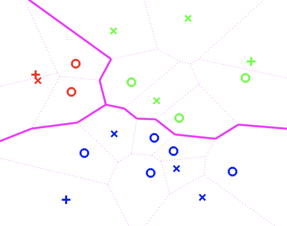
(a) 20 Robots, 3 Regions

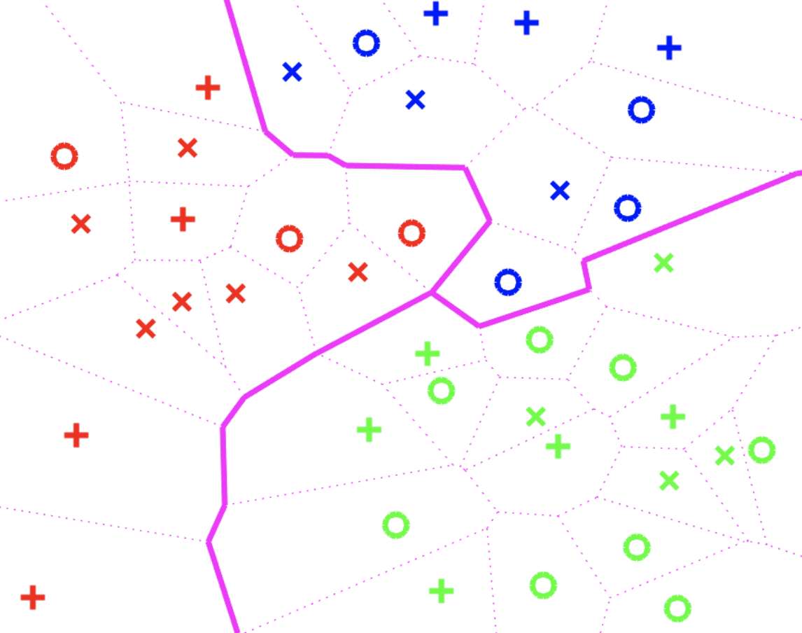
(b) 40 Robots, 3 Regions

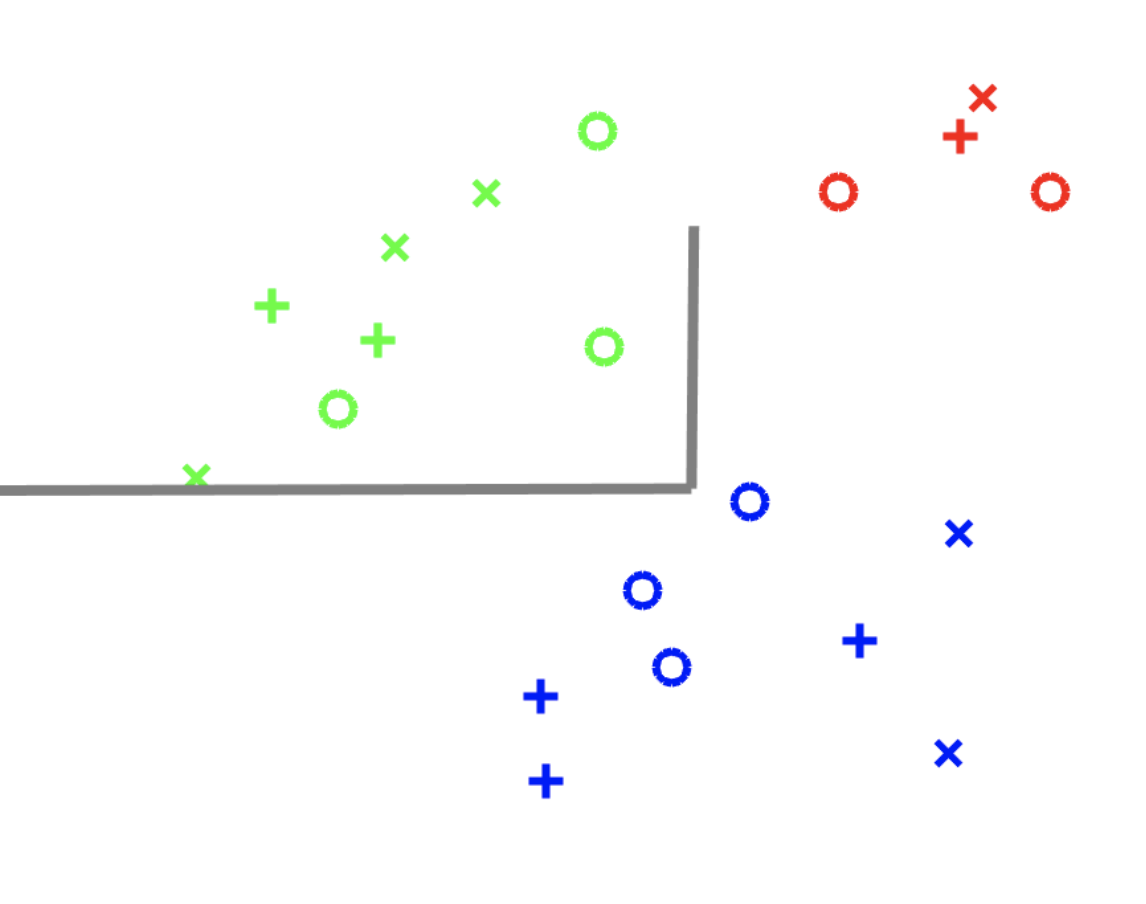
(c) 20 Robots, 3 Regions

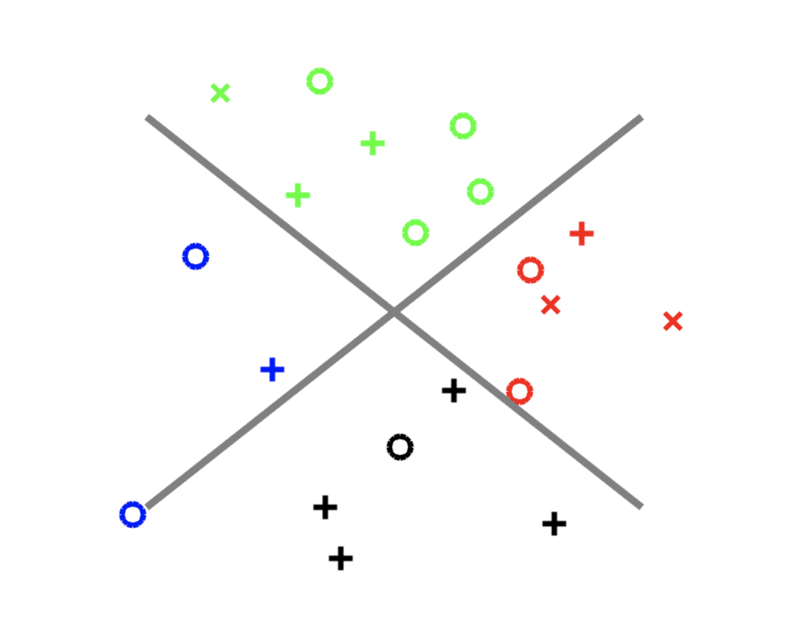
(d) 20 Robots, 4 Regions

Figure 1: Figures 1(a) and 1(b) show coverage regions for varying number of robots. Light dotted magenta lines show the spacing of individual robots, while bold magenta lines depict the coverage regions of the heterogeneous teams. Figures 1(c) and 1(d) show our approach’s performance with obstacles in the environment (marked with gray lines). Voronoi regions are not marked here to reduce visual noise. Markers show individual robots, with the marker color denoting the team assignment and the marker shape indicating that robot’s capability (e.g., a robot marked by an ‘o’ has different sensing capability than a robot marked by an ‘x’).

Convergence and complexity

The general ALM method described and on which our solution is based is proven to converge to an optimal solution [41] as long as $0<\mu^{k}<\mu^{k+1}$ for iteration $k$. With this assumption, the current solution $\mathbf{X}^{k}$ will approach the optimal solution $\mathbf{X}^{k*}$. Since we initialize $\mu^{0}$ to be positive, initialize $\rho$ such that $1<\rho<2$, and update $\mu$ by $\mu^{k+1}=\rho\mu^{k}$ (Line 10 in Algorithm 1), this assumption will hold at every iteration. In terms of complexity, it is trivial to update $\mathbf{\phi}_{1}$, $\mathbf{\Phi}_{2}$, $\mathbf{\Phi}_{3}$, and $\mathbf{\Phi}_{4}$ in Lines 6-9, as well as $\mu$ and $k$ in Lines 10 and 11. The time complexity of our solution is dominated by the update of $\mathbf{Z}$ in Line 3, $\hat{\mathbf{Z}}$ in Line 4, and $\mathbf{L}$ in Line 5. Lines 3 and 4 compute a matrix inverse and multiplication, each of complexity $\mathcal{O}(N^{3})$. Line 5 calculates the SVD of a square matrix, also with a complexity of $\mathcal{O}\left(N^{3}\right)$. As a result, the overall complexity of our solution is $\mathcal{O}\left(N^{3}\right)$.

V Experimental Results

We evaluated on both simulated and physical multi-robot systems, each described with three different graphs representing their heterogeneous relationships.

1. Spatial relationship: The first graph, $\mathcal{G}_{S}$, describes the spatial structure of the system. Each edge $e_{ij}$ describes the inverse of the distance between the $i$-th and the $j$-th robot, causing nearby robots to have higher edge weights than further apart robots.

2. Communication: The second graph, $\mathcal{G}_{C}$, describes the communication capabilities of the system. Robots are physically limited in their communication capabilities, just as they are limited in their sensing capabilities. For this graph, $e_{ij}=1$ if the $i$-th robot is able to communicate to the $j$-th robot, and $0$ if not.

3. Heterogeneous sensing capability: The third graph, $\mathcal{G}_{SC}$, describes the relationships between robots based on their sensing capabilities. We define a set of sensing capabilities $\mathcal{C}$, with $\mathcal{C}_{i}$ denoting the capabilities of the $i$-th robot. $\mathcal{G}_{SC}$ represents the similarity of two robots based on their relative sensing capabilities. Here, $e_{ij}=|\mathcal{C}_{i}\cap\mathcal{C}_{j}|$, or the size of the intersection between the $i$-th robot’s capabilities and the $j$-th robot’s capabilities.

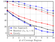
(a) 20 Robots, 3 Capabilities

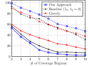
(b) 20 Robots, 5 Capabilities

(c) 40 Robots, 3 Capabilities

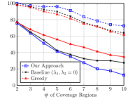
(d) 40 Robots, 5 Capabilities

Figure 2: Event detection and robot duplication as the number of coverage regions varies, for simulated multi-robot systems of $N=\{20,40\}$ and $|\mathcal{C}|=\{3,5\}$. Dashed lines indicate event detection, where higher rates are the better result, while solid lines indicate robot duplication, where lower rates are better.

We adopt two metrics commonly used in multi-robot sensor coverage literature for evaluation, as well as a new metric to quantitatively evaluate the composition of our identified teams.

1. Voronoi diagrams are adopted as a metric to evaluate the coverage regions assigned to each heterogeneous team. Voronoi regions divide an area into polygons based on the distance to different points, and are commonly used to qualitatively assess robot coverage methods [2, 8].

2. Event detection is used to evaluate sensing quality. For each testing iteration we simulate 100 events of multiple types, each of which is detectable by a single sensing capability, following [11, 8]. If an event occurs in a region where a robot team member has the sensing ability to sense that type of event, then the event is considered detected. If no such robot exists, then the event is not detected. An event detection rate of $100\%$ is optimal, meaning all events are detected.

3. Robot duplication is introduced to evaluate the composition of the identified teams. If a team contains two robots that share a sensor capability, then one robot is a duplicate. The sensor duplication score is $\frac{d}{n}$, where $d$ is the number of duplicate robots and $n$ is the total number of robots. Lower duplication rates are better, as this corresponds to robots being more evenly distributed.

We compare our approach to a baseline version as well as a greedy algorithm. The baseline version of our approach sets $\lambda_{1}=\lambda_{2}=0$, so that our learned representation matrix $\mathbf{Z}$ is still constrained to be bistochastic but does not utilize the two regularization terms that induce a block structure. The greedy algorithm disregards sensor capability relationships and assigns robots to a region purely based on spatial relationships, i.e. robots near each other are assigned to the same team.

V-A Results on Simulated Multi-Robot Systems

We simulated systems of $N=\{10,20,30,40,50\}$ robots, and randomly assign a varying number of sensing capabilities for $|\mathcal{C}|=\{2,3,4,5\}$. The graphs describing each system were defined based on the generated positions and capabilities.

Figures 1(a) and 1(b) show qualitative results for two instances of these simulations in the form of Voronoi diagrams for 20 and 40 robots assigned into 3 teams. While we show the boundaries between individual robots, our approach assigns teams that cover larger regions together, indicated by the bold magenta Voronoi lines. Figures 1(c) and 1(d) show team assignment results in the presence of obstacles, with walls indicated by the gray lines. These obstacles alter the spatial and communication relationships among robots, i.e., robots separated by a wall cannot communicate. It can be seen that our approach is able to assign teams which are not separated by walls which would interfere with cooperative operation.

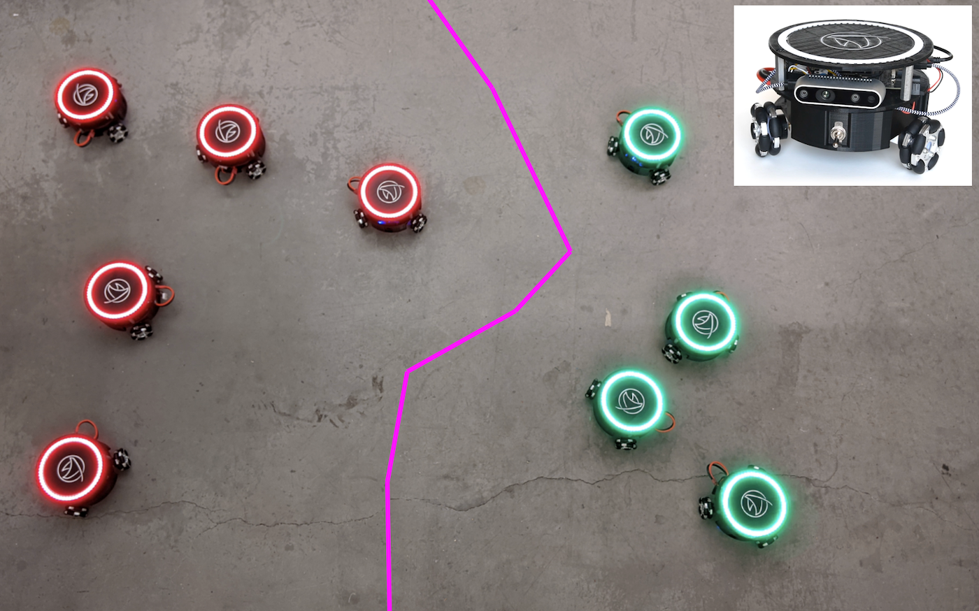
(a) 2 Regions

(b) 3 Regions

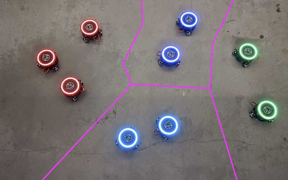
(c) 4 Regions

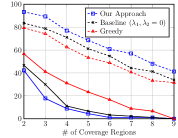
(d) Quantitative

Figure 3: Results from our evaluation on physical robots. Figures 3(a)–3(c) show robots assigned to teams to cover 2, 3, and 4 regions. The magenta lines indicate the separation between Voronoi regions that each team of robots is assigned to cover, while the LED rings on the robots indicate teams. Figure 3(d) shows the event detection (dashed lines) and robot duplication (solid line) rates for the physical robot system.

Figure 2 shows the results for the event detection metric for a subset of the simulations, specifically $N=\{20,40\}$ and $|\mathcal{C}|=\{3,5\}$ and covering between 2 and 10 regions. We see that in most cases, the baseline version of our approach outperforms the greedy algorithm based only on spatial relationships. However, our approach consistently outperforms both, showing that the block structure induced in the unified representation matrix corresponds well to teams with high event detection rates. Although not displayed due to space limitations, these results are consistent with those for other values of $N$ and $|\mathcal{C}|$.

Figure 2 also shows results from the robot duplication metric. We observe that in all tested cases in the experiments, our approach outperforms the greedy approach based purely upon distance between robots as well as a baseline version of our approach. The teams identified by our approach contain consistently fewer robots with duplicate sensing capabilities, demonstrating that our approach is effective at distributing capabilities among teams.

V-B Results on Physical Multi-Robot Systems

Our second experiment implements our approach on physical robots using our multi-robot platform, consisting of $N=9$ robots. Each robot, seen in the top corner of Figure 3(a), is equipped with an RGB camera, depth camera, and microphone for $|\mathcal{C}|=3$ sensing capabilities, as well as an LED ring for status indication. We randomly disabled sensing capabilities on the robots, so that each individual robot was limited to a single capability. Robots moved randomly, with team assignments and simulated events occurring at discrete time steps. Figures 3(a)–3(c) show sample team assignments for 2 to 4 regions.

Figure 3(d) shows the results of this evaluation in terms of event detection and robot duplication. We see that our full approach outperforms the others by a greater margin that on the larger simulated systems, suggesting that the heterogeneous relationships our approach learns from are especially influential on smaller scales. In terms of robot duplication, our approach again outperforms the baseline approach and the greedy approach. We note that the baseline approach very closely tracks the performance of our full approach when the number of regions is four or greater, suggesting that the block structure induced by our full approach has a limited influence as the blocks grow smaller (i.e., the number of robots on each team decreases). We also see that all three approaches converge at duplication of $0\%$ when the number of teams equals the number of robots; when only a single robot is present in each region, there can be no duplicates.

V-C Hyperparameter Analysis

We analyze the influence of the hyperparameters that control the importance of each input graph, including $\alpha_{1}$ (controlling the importance of the spatial graph), $\alpha_{2}$ (the communication graph), and $\alpha_{3}$ (the sensing capability graph). Figure 4 shows the event detection and robot duplication rates on a simulated multi-robot system resulting from various combinations of the hyperparameters, in the triangular topological space [42] with each side of the triangle corresponding to an $\alpha_{i}\in[0,1]$ and $\sum_{i=1}^{3}\alpha_{i}=1$ with 2 independent values out of 3. For example, the black cross in Figure 4(a), marking the best event detection rate, represents $\alpha_{1}=0.2$, $\alpha_{2}=0.1$, and $\alpha_{3}=0.7$.

In Figure 4(a), the event detection is at its highest for high values of $\alpha_{3}$, demonstrating the importance of the sensing capabilities graph. We observe that balancing $\alpha_{1}$ and $\alpha_{2}$ in the bottom right corner can maintain middling performance, but relying solely on either of them causes event detection rates to fall to their lowest values below $55\%$. Figure 4(b) shows similar but much more consistent effects when evaluating the rate of robot duplication, with high values of $\alpha_{3}$ ($>0.6$) corresponding to low rates of duplication ($<20\%$). Furthermore, we see that high values of $\alpha_{2}$ cause higher rates of duplication, suggesting that grouping nearby robots is a poor way to ensure heterogeneous teams.

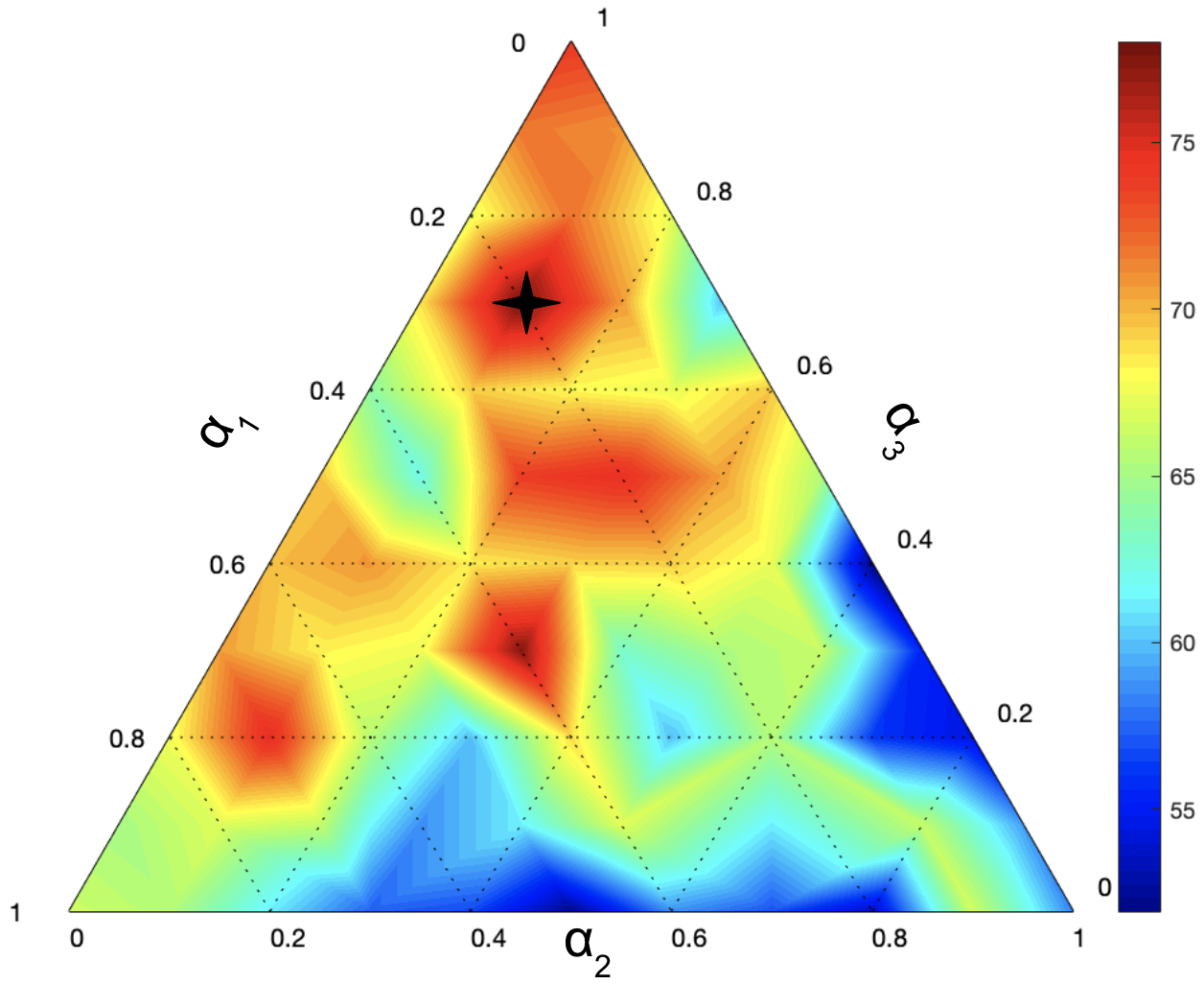
(a) Event Detection

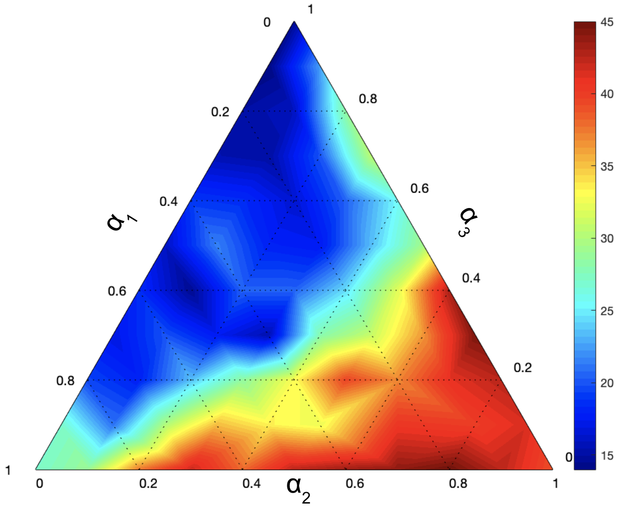
(b) Robot Duplication

Figure 4: Evaluation of the effect of hyperparameters on the event detection and robot duplication rates. For event detection, a high rate (in red) is good, whereas for robot duplication, a low rate (in blue) is better.

VI Conclusion

As real-world robots in a multi-robot system are typically limited in their individual sensing capabilities, coverage of an area by a heterogeneous multi-robot system requires the effective assignment of teams that contain a variety of capabilities. We propose an approach to learn a unified representation of the heterogeneous relationships in the system, utilizing natural divisions to assign teams. We show that our approach identifies teams with high rates of event detection and low duplication of robot capabilities.

References

- [1] J. Cortes, S. Martinez, T. Karatas, and F. Bullo, “Coverage control for mobile sensing networks,” Transactions on Robotics and Automation, vol. 20, no. 2, pp. 243–255, 2004.
- [2] W. Luo and K. Sycara, “Adaptive sampling and online learning in multi-robot sensor coverage with mixture of gaussian processes,” in International Conference on Robotics and Automation, 2018.
- [3] M. Schwager, J. McLurkin, and D. Rus, “Distributed coverage control with sensory feedback for networked robots.,” in Robotics: Science and Systems, 2006.
- [4] S. Meguerdichian, F. Koushanfar, G. Qu, and M. Potkonjak, “Exposure in wireless ad-hoc sensor networks,” in International Conference on Mobile Computing and Networking, 2001.
- [5] V. Zadorozhny and M. Lewis, “Information fusion based on collective intelligence for multi-robot search and rescue missions,” in International Conference on Mobile Data Management, 2013.
- [6] W. Luo, S. S. Khatib, S. Nagavalli, N. Chakraborty, and K. Sycara, “Distributed knowledge leader selection for multi-robot environmental sampling under bandwidth constraints,” in International Conference on Intelligent Robots and Systems, 2016.
- [7] L. E. Parker, Heterogeneous Multi-Robot Cooperation. PhD thesis, Massachusetts Institute of Technology, 1994.
- [8] M. Santos and M. Egerstedt, “Coverage control for multi-robot teams with heterogeneous sensing capabilities using limited communications,” in International Conference on Intelligent Robots and Systems, 2018.
- [9] B. Reily, C. Reardon, and H. Zhang, “Representing multi-robot structure through multimodal graph embedding for the selection of robot teams,” in International Conference on Robotics and Automation, 2020.
- [10] A. Pierson, L. C. Figueiredo, L. C. Pimenta, and M. Schwager, “Adapting to sensing and actuation variations in multi-robot coverage,” International Journal of Robotics Research, vol. 36, no. 3, pp. 337–354, 2017.
- [11] A. Sadeghi and S. L. Smith, “Coverage control for multiple event types with heterogeneous robots,” in International Conference on Robotics and Automation, 2019.
- [12] I. Rekleitis, A. P. New, E. S. Rankin, and H. Choset, “Efficient boustrophedon multi-robot coverage: an algorithmic approach,” Annals of Mathematics and Artificial Intelligence, vol. 52, no. 2-4, pp. 109–142, 2008.
- [13] N. Fung, J. Rogers, C. Nieto, H. I. Christensen, S. Kemna, and G. Sukhatme, “Coordinating multi-robot systems through environment partitioning for adaptive informative sampling,” in International Conference on Robotics and Automation, 2019.
- [14] M. Corah and N. Michael, “Efficient online multi-robot exploration via distributed sequential greedy assignment.,” in Robotics: Science and Systems, 2017.
- [15] S.-k. Yun and D. Rus, “Distributed coverage with mobile robots on a graph: locational optimization and equal-mass partitioning,” Robotica, vol. 32, no. 2, pp. 257–277, 2014.
- [16] S.-k. Yun and D. Rusy, “Distributed coverage with mobile robots on a graph: Locational optimization,” in International Conference on Robotics and Automation, 2012.
- [17] J. Cortés, S. Martinez, T. Karatas, and F. Bullo, “Coverage control for mobile sensing networks: Variations on a theme,” in Mediterranean Conference on Control and Automation, 2002.
- [18] S. G. Lee, Y. Diaz-Mercado, and M. Egerstedt, “Multirobot control using time-varying density functions,” Transactions on Robotics, vol. 31, no. 2, pp. 489–493, 2015.
- [19] K. Guruprasad and D. Ghose, “Automated multi-agent search using centroidal voronoi configuration,” Transactions on Automation Science and Engineering, vol. 8, no. 2, pp. 420–423, 2010.
- [20] K. Guruprasad and D. Ghose, “Performance of a class of multi-robot deploy and search strategies based on centroidal voronoi configurations,” International Journal of Systems Science, vol. 44, no. 4, pp. 680–699, 2013.
- [21] S. Manjanna, A. Q. Li, R. N. Smith, I. Rekleitis, and G. Dudek, “Heterogeneous multi-robot system for exploration and strategic water sampling,” in International Conference on Robotics and Automation, 2018.
- [22] F. Shkurti, A. Xu, M. Meghjani, J. C. G. Higuera, Y. Girdhar, P. Giguere, B. B. Dey, J. Li, A. Kalmbach, C. Prahacs, et al., “Multi-domain monitoring of marine environments using a heterogeneous robot team,” in International Conference on Intelligent Robots and Systems, 2012.
- [23] S. Hood, K. Benson, P. Hamod, D. Madison, J. M. O’Kane, and I. Rekleitis, “Bird’s eye view: Cooperative exploration by ugv and uav,” in International Conference on Unmanned Aircraft Systems, 2017.
- [24] O. Arslan and D. E. Koditschek, “Voronoi-based coverage control of heterogeneous disk-shaped robots,” in International Conference on Robotics and Automation, 2016.
- [25] K. Guruprasad and D. Ghose, “Heterogeneous locational optimisation using a generalised voronoi partition,” International Journal of Control, vol. 86, no. 6, pp. 977–993, 2013.
- [26] P. Gao, Z. Zhang, R. Guo, H. Lu, and H. Zhang, “Correspondence identification in collaborative robot perception through maximin hypergraph matching,” in International Conference on Robotics and Automation, 2020.
- [27] P. Gao, R. Guo, H. Lu, and H. Zhang, “Regularized graph matching for correspondence identification under uncertainty in collaborative perception,” in Robotics: Science and Systems, 2020.
- [28] M. Schwager, D. Rus, and J.-J. Slotine, “Decentralized, adaptive coverage control for networked robots,” International Journal of Robotics Research, vol. 28, no. 3, pp. 357–375, 2009.
- [29] J. Le Ny and G. J. Pappas, “Adaptive deployment of mobile robotic networks,” Transactions on Automatic Control, vol. 58, no. 3, pp. 654–666, 2012.
- [30] M. Santos, Y. Diaz-Mercado, and M. Egerstedt, “Coverage control for multirobot teams with heterogeneous sensing capabilities,” Robotics and Automation Letters, vol. 3, no. 2, pp. 919–925, 2018.
- [31] I. Jang, H.-S. Shin, and A. Tsourdos, “Anonymous hedonic game for task allocation in a large-scale multiple agent system,” Transactions on Robotics, vol. 34, no. 6, pp. 1534–1548, 2018.
- [32] I. Jang, H.-S. Shin, and A. Tsourdos, “A comparative study of game-theoretical and markov-chain-based approaches to division of labour in a robotic swarm,” International Federation of Automatic Control, vol. 51, no. 12, pp. 62–68, 2018.
- [33] A. Brutschy, G. Pini, C. Pinciroli, M. Birattari, and M. Dorigo, “Self-organized task allocation to sequentially interdependent tasks in swarm robotics,” in Autonomous Agents and Multi-Agent Systems, 2014.
- [34] M. Castillo-Cagigal, A. Brutschy, A. Gutiérrez, and M. Birattari, “Temporal task allocation in periodic environments,” in International Conference on Swarm Intelligence, 2014.
- [35] I. Rekleitis, V. Lee-Shue, A. P. New, and H. Choset, “Limited communication, multi-robot team based coverage,” in International Conference on Robotics and Automation, 2004.
- [36] M. Schneider-Fontan and M. J. Mataric, “Territorial multi-robot task division,” Transactions on Robotics and Automation, vol. 14, no. 5, pp. 815–822, 1998.
- [37] T. H. Labella, M. Dorigo, and J.-L. Deneubourg, “Division of labor in a group of robots inspired by ants’ foraging behavior,” Transactions on Autonomous and Adaptive Systems, vol. 1, no. 1, pp. 4–25, 2006.
- [38] H. Wu, H. Li, R. Xiao, and J. Liu, “Modeling and simulation of dynamic ant colony’s labor division for task allocation of uav swarm,” Physica A: Statistical Mechanics and Its Applications, vol. 491, pp. 127–141, 2018.
- [39] E. Bonabeau, A. Sobkowski, G. Theraulaz, J.-L. Deneubourg, et al., “Adaptive task allocation inspired by a model of division of labor in social insects,” in Bio-Computing and Emergent Computation, pp. 36–45, 1997.
- [40] M. Fiedler, “Algebraic connectivity of graphs,” Czechoslovak Mathematical Journal, vol. 23, no. 2, pp. 298–305, 1973.
- [41] D. P. Bertsekas, Constrained optimization and Lagrange multiplier methods. Academic Press, 2014.
- [42] H. Zhang, W. Zhou, C. Reardon, and L. E. Parker, “Simplex-based 3d spatio-temporal feature description for action recognition,” in Computer Vision and Pattern Recognition, 2014.