Space Occupancy in Low-Earth Orbit

Claudio Bombardelli

Technical University of Madrid (UPM), Madrid, 28040, Spain,

Gabriele Falco

University of Naples Federico II, Naples, 80125, Italy,

Davide Amato

University of Colorado, Boulder, CO 80309,

and

Aaron J. Rosengren

UC San Diego, La Jolla, CA 92093

abstract

With the upcoming launch of large constellations of satellites in the low-Earth orbit (LEO) region it will become important to organize the physical space occupied by the different operating satellites in order to minimize critical conjunctions and avoid collisions. Here, we introduce the definition of space occupancy as the domain occupied by an individual satellite as it moves along its nominal orbit under the effects of environmental perturbations throughout a given interval of time. After showing that space occupancy for the zonal problem is intimately linked to the concept of frozen orbits and proper eccentricity, we provide frozen-orbit initial conditions in osculating element space and obtain the frozen-orbit polar equation to describe the space occupancy region in closed analytical form. We then analyze the problem of minimizing space occupancy in a realistic model including tesseral harmonics, third-body perturbations, solar radiation pressure, and drag. The corresponding initial conditions, leading to what we call minimum space occupancy (MiSO) orbits, are obtained numerically for a set of representative configurations in LEO. The implications for the use of MiSO orbits to optimize the design of mega-constellations are discussed.

Introduction

Preserving and sustaining the Low Earth Orbit (LEO) environment as a valuable resource for future space users has motivated space actors to consider mechanisms to control the growth of man-made debris. These prevention, mitigation, and remediation actions will become more and more urgent following the launch of upcoming mega-constellations of satellites to provide high-bandwidth, space-based internet access. Envisioned mega-constellation designs involve the deployment of thousands of satellite at nominally equal altitude and inclination and distributed over a number of orbital planes for optimized ground coverage. The concentration of such a high number of satellites in a relatively small orbital region can lead to a high risk of in-orbit collisions and an escalation of required collision avoidance maneuvers[1, 2, 3]. In this scenario, any design solution that can limit potential collisions and required maneuvers as much as possible would be highly welcomed.

A possible collision mitigation action that can be implemented at a negligible cost for space operators is to minimize the potential interference of a satellite with the rest of its constellation members by a judicious orbit design within the limits imposed by mission requirements. Ideally, if each individual satellite could be confined to within a region of space with zero overlap between the rest of the constellation members, the endogenous collision risk and frequency of collision avoidance maneuvers of a constellation of satellites would be reduced to zero.

In a perturbation-free environment, the obvious solution would be to adopt a sequence of orbits of equal eccentricity, but slightly different semi-major axes. Considering a more accurate model that includes zonal harmonic perturbations, non-intersecting orbits can still be achieved by placing the individual satellites in non-overlapping frozen orbits of slightly different semi-major axes. Frozen orbits (see [4] and references therein) show the remarkable property of having constant altitude at equal latitude which is a consequence of the fact that their singly-averaged eccentricity, argument of pericenter, and inclination, are constant.

When tesseral harmonics, third-body effects, and non-gravitational perturbations are accounted for, perfectly frozen orbits cease to exist, which makes it impossible to achieve control-free, constant-altitude orbital motion at equal latitude. Accordingly, one can attempt to minimize residual altitude oscillations by adopting initial conditions near to the ones corresponding to a frozen orbit in the zonal problem and to approach the absolute minimum by a slight variation of the initial state vector. To our knowledge, there has been no effort in the available literature to obtain initial conditions leading to an absolute minimum of the altitude variations of a LEO orbiting spacecraft in a given time span. Note that quasi-frozen orbits including tesseral harmonics, third-body perturbations and solar radiation pressure have been obtained in the literature using a double-averaging approach ([6, 7, 8, 9]), which certainly provides an increase in orbit lifetime and stability but does not necessarily lead to a minimization of altitude oscillations at equal latitude.

In this article, we employ analytical and numerical methods to study what we call “space occupancy range” (SOR), “space occupancy area” (SOA), and “space occupancy volume” (SOV) of a satellite in LEO. The first quantity corresponds to the extent of the equal-latitude radial displacement of the satellite in a given time span, while the second and third represent, respectively, the total surface area and volume swept by the satellite throughout a given time span as it moves in its osculating orbital plane (SOA) or in the orbital space (SOV). Moreover, we employ a high-fidelity numerical algorithm to determine MiSO initial conditions for an orbit with a given semi-major axis and inclination. Once these initial conditions are established and the dynamical behavior of these orbits is well understood, we propose to organize the orbital space of future mega-constellations by distributing the different satellites in non-overlapping MiSO shells thus minimizing the number of critical conjunctions between satellites of different orbital planes, and, consequently, the frequency of collision avoidance maneuvers.

The structure of the article is the following. First, we provide a definition of space occupancy and review frozen-orbit theory for the zonal problem starting from the seminal 1966 article by Cook [10]. Next, we show how space occupancy can be directly related to the concept of proper eccentricity. We then derive simple analytical formulas to obtain near-frozen initial conditions in osculating element space based on the Kozai-Brower-Lyddane mean-to-osculating element transformations and obtain a compact and accurate analytical expression for the polar equation of a frozen orbit in the zonal problem.

In the last section of the article, we investigate space occupancy considering a high-fidelity model including high-order tesseral harmonics, lunisolar perturbations and non-gravitational perturbations (solar radiation pressure and drag). It is important to underline that an accurate modeling of the Earth attitude and rotation (including precession, nutation and polar motion) is taken into account when computing high-order tesseral harmonics.

Numerical simulations are conducted in order to obtain minimum space occupancy initial conditions and map the minimum achievable space occupancy for different altitudes and inclinations in LEO. The time evolution of the space occupancy of MiSO orbits under the effect of environmental perturbations is also investigated in detail. Finally, the implications of these results on the design of minimum-conjunction mega-constellations of satellites for future space-based internet applications are discussed.

Space Occupancy: Definition

We define the space occupancy range of an orbiting body, of negligible size compared to its orbital radius, over the interval $\left[t_{0},\,t_{0}+\Delta t\right]$, as the maximum altitude variation for fixed latitude experienced by the body throughout that time interval:

$$\mathrm{SOR}\left(t_{0},\Delta t\right)=\max\left\{\Delta r\left(\phi\right),\phi\in\left[0,\phi_{max}\right],t\in\left[t_{0},\,t_{0}+\Delta t\right]\right\}$$

where the maximum reachable latitude $\phi_{max}$ can be taken, with good approximation, as the mean orbital inclination $\hat{i}$.

Based on the preceding definition, there are two ways of following the time evolution of the SOR, depending whether $t_{0}$ or $\Delta t$ is held constant, which leads to the definition of a cumulative vs. fixed-timespan SOR function. The cumulative SOR is a monotonic function of the time span $\Delta t$ that describes how a spacecraft, starting from a fixed epoch $t_{0}$, occupies an increasing range of radii as its orbit evolves in time under the effect of the different perturbation forces. Conversely, the fixed-timespan SOR is a function that measures how the SOR changes as the initial epoch of the measurement interval moves forward in time while the timespan $\Delta t$ is held fixed.

We define the space occupancy area over the interval $\left[t_{0},\,t_{0}+\Delta t\right]$, as the smallest two-dimensional region in the mean orbital plane containing the motion of the orbiting body as its orbit evolves throughout that time interval.

Finally, we define the space occupancy volume over the interval $\left[t_{0},\,t_{0}+\Delta t\right]$, as the volume swept by the SOA when the orbital plane precesses around the polar axis of the primary body.

When the most important perturbation terms are those stemming from the zonal harmonic potential with a dominant second order ($J_{2}$) term, as it is in the case of LEO, the SOA is an annulus of approximately constant thickness and whose shape will be shown, in this article, to correspond to an offset ellipse. Under the same hypothesis the SOV takes the shape of a barrel whose characteristics will also be studied.

Frozen Orbits for the Zonal Problem

The theory of frozen orbits was pioneered by Graham E. Cook in his seminal 1966 paper [10]. Here, we summarize Cook’s equations and their implications for the space occupancy concept. In line with Cook, the dynamical model we refer to in this section accounts for the effect of $J_{2}$ plus an arbitrary number of odd zonal harmonics.

Let us employ dimensionless units of length and time, taking the Earth radius $R_{\oplus}$ as the reference length and $1/n_{\oplus}$ as the reference time with $n_{\oplus}$ indicating the mean motion of a Keplerian circular orbit of radius $R_{\oplus}$. Let us indicate with $\hat{e}$, $\hat{\omega}$, $\hat{a}$, $\hat{n}$ and $\hat{i}$ the mean value (i.e., averaged over the mean anomaly) of the eccentricity, argument of periapsis, semi-major axis, mean motion and inclination, respectively, where the latter is considered constant after neglecting its small-amplitude long-periodic oscillations.

The differential equations describing the evolution of the mean eccentricity vector perifocal components, $\xi=\hat{e}\cos\hat{\omega}$ and $\eta=\hat{e}\sin\hat{\omega}$, are [10]:

$$\left\{\begin{array}[]{c}\dot{\xi}=-k\left(\eta+e_{f}\right),\\ \\ \dot{\eta}=k\xi,\end{array}\right.$$ (1)

where:

$$k=\frac{3\hat{n}J_{2}}{\hat{a}^{3}}\left(1-\frac{5}{4}\sin^{2}\hat{i}\right),$$

and $e_{f}$, known as frozen eccentricity, can be expressed as [10]:

$$e_{f}=k^{-1}\hat{a}_{0}^{-3/2}\sum_{n=1}^{N}\frac{J_{2n+1}}{\hat{a}_{0}^{2n+1}}\frac{n}{\left(2n+1\right)\left(n+1\right)}P_{2n+1}^{1}(0)P_{2n+1}^{1}(\cos\hat{i})=-\frac{J_{3}}{2J_{2}}\frac{\sin\hat{i}}{\hat{a}}+o\left(J_{3}/J_{2}\right),$$ (2)

with $P_{n}^{1}$ indicating the associated Legendre function of order one and degree $n$.

The solution of Eqs. (1) is:

$$\left\{\begin{array}[]{c}\xi\left(\tau\right)=e_{p}\cos\left(k\tau+\alpha\right),\\ \\ \eta\left(\tau\right)=e_{p}\sin\left(k\tau+\alpha\right)+e_{f},\end{array}\right.$$ (3)

where:

$$e_{p}=\sqrt{\left(\hat{e}_{0}\sin\hat{\omega}_{0}-e_{f}\right)^{2}+\hat{e}_{0}^{2}\cos^{2}\hat{\omega}_{0}},$$ (4)

$$\sin\alpha=\frac{\hat{e}_{0}\sin\hat{\omega}_{0}-e_{f}}{e_{p}},\qquad\cos\alpha=\frac{\hat{e}_{0}\cos\hat{\omega}_{0}}{e_{p}}.$$

Eqs.(3) corresponds to a circle of radius $e_{p}$, which is a constant today known as the proper eccentricity, and center $\left(0,e_{f}\right)$ in the $\xi-\eta$ plane. By selecting as initial conditions $\hat{\omega}_{0}=\pi/2$ and $\hat{e}_{0}=e_{f}$ the circle reduces to a point and both $\hat{\omega}$ and $\hat{e}$ remain constant, implying that their long-periodic oscillations have been eliminated and yielding what is known as a frozen orbit. Note that long-periodic oscillations of the inclination and mean anomaly are also removed under the frozen orbit conditions as it is evident from [11, page 394].

Space Occupancy for the Zonal Problem

One remarkable feature of frozen orbits is that they have a constant altitude for a given latitude. This is a consequence of the fact that the long-periodic variations in the magnitude and direction of the eccentricity vector are (within the validity of the averaging approximation) identically zero.

That feature can be shown mathematically by writing the orbital radius as:

$$r=\frac{\left(\hat{a}+a_{sp}\right)\left(1-\left(\hat{e}+e_{sp}\right)^{2}\right)}{1+\left(\hat{e}+e_{sp}\right)\cos\nu},$$

where $a_{sp}$ and $e_{sp}$ are the short-periodic components of, respectively, the semi-major axis and eccentricity and $\nu$ is the osculating true anomaly.

Since all short-periodic components are small quantities we can write:

$$r=\hat{r}+r_{sp}\approx\frac{\hat{a}\left(1-\hat{e}^{2}\right)}{1+\hat{e}\cos\nu}+\left(\frac{1-\hat{e}^{2}}{1+\hat{e}\cos\nu}a_{sp}-\frac{\hat{a}\left[2\hat{e}+\left(1+\hat{e}^{2}\right)\cos\nu\right]}{\left(1+\hat{e}\cos\nu\right)^{2}}e_{sp}\right),$$ (5)

In the above equation $r_{sp}$ and $\hat{r}$ are, respectively, the fast- and slow-scale of the orbit radius variation.

On the other hand, the relation between the orbit latitude, $\phi$, and true anomaly reads:

$$\frac{\sin\phi}{\sin i}=\sin\left(\nu+\omega\right).$$ (6)

For a frozen orbit, $\hat{e}$ is a constant and, since $\hat{\omega}$ is also constant and equal to $\pi/2$, both $a_{sp}$ and $e_{sp}$ are periodic functions with $\cos\nu$, $\cos 2\nu$ and $\cos 3\nu$ terms [12]. This means that both $\hat{r}$ and $r_{sp}$ are explicit functions of $\nu$. Moreover, under frozen-orbit conditions and neglecting short-periodic oscillations of $i$ (i.e., $i\simeq\hat{i}=\mathrm{const}$) as well as short-periodic oscillations of $\omega$ (i.e. , $\omega\simeq\hat{\omega}=\pi/2$) the true anomaly $\nu$ is, following Eq. (6), an explicit function of $\phi$:

$$\nu\approx\cos^{-1}\left(\frac{\sin\phi}{\sin\hat{i}}\right).$$

This proves that for a frozen orbit the terms $\hat{r}$ and $r_{sp}$ in Eq.(5) are explicit functions of $\phi$ and the SOR is zero.

When frozen conditions are not met the term $\hat{r}$ is no longer an explicit function of $\nu$ owing to the long-periodic variations of $\hat{e}$. Likewise $\nu$ is no longer an explicit function of $\phi$ owing to the long-periodic variations of $\hat{\omega}$. Neglecting the contribution of $r_{sp}$ compared to $\hat{r}$, the SOR corresponds to the maximum “mean” apoapsis minus the minimum “mean” periapsis, and, accounting for Cook’s solution (Eq.(3)):

$$\mathrm{SOR}=\left(\Delta r\right)_{\max}\approx\hat{a}_{0}\left(\hat{e}_{\max}-\hat{e}_{\min}\right)=2\hat{a}e_{p},$$

showing that space occupancy in the zonal problem is fundamentally related to the proper eccentricity, $e_{p}$, of the orbit. Note that when $\hat{e}_{0}>>e_{f}$ one has $e_{p}\simeq\hat{e}_{0}$ as it is evident from Eq. (4).

Frozen Orbit Dynamics and Geometry

In order to fully characterize space occupancy we will now obtain simple relations characterizing the geometry of frozen orbits. In order to do that one needs to view frozen orbits in osculating elements space using the mean-to-osculating orbital elements conversion formulas ([12, 13]) reported, for convenience, in Appendix I.

Maximum-Latitude Conditions

Owing to the axial symmetry of the zonal problem and their periodic nature, frozen orbits are axially symmetric. Therefore, at the maximum latitude ($\omega+\nu=\pi/2$) the satellite must be either at periapsis ($\omega=\pi/2$, $M=\nu=0$) or apoapsis ($\omega=3\pi/2$, $M=\nu=\pi$) of its osculating orbit. Consequently, the computation of the frozen orbit initial conditions is very convenient when referring to the maximum latitude point.

Following Kozai’s [12], the osculating eccentricity can be written as a sum of a mean and a short-periodic term:

$$e=\hat{e}+e_{sp},$$

where the short-periodic component $e_{sp}$ is dominated by the $J_{2}$ perturbation and obeys Eq. (16) given in Appendix I.

In frozen orbit conditions $\hat{e}=e_{f}$ and $\hat{\omega}=\pi/2$. In addition, the mean true anomaly, here denoted with $\hat{\nu}$, must be zero at the maximum latitude point for symmetry. From Eq. (16) the short-periodic part of the eccentricity at maximum latitude (subindex “$N$” as in “North” ) yields, after neglecting second order terms in $e_{f}$ and $J_{2}$:

$$e_{sp,N}\approx\frac{J_{2}}{2\hat{a}^{2}}\left(7\cos^{2}\hat{i}-4\right),$$

By setting the previous expression to $-e_{f}$ and solving for $\hat{i}$ one obtains the inclination value at which the maximum-latitude osculating orbit becomes circular:

$$e_{N}=e_{sp,N}+e_{f}=0\;\mathrm{for\;\mathit{\begin{cases}\hat{i}=\hat{i}^{*},\\ \hat{i}=\pi-\hat{i}^{*},\end{cases}}}$$ (7)

with:

$$\hat{i}^{*}\approx\cos^{-1}\left(\sqrt{\frac{2}{7}\left(2-\frac{\hat{a}^{2}e_{f}}{J_{2}}-\frac{15e_{f}}{4}\right)}\right).$$

For the LEO case with altitudes between 400 and 2000 km, $\hat{i}^{*}$ oscillates between $\sim 41{}^{\circ}$ and $\sim 66^{\circ}$ depending mainly on $\hat{i}$ .

By considering the short-periodic part of the argument of periapsis (see Eq.(27) in Appendix I):

$$\tilde{\omega}_{sp,N}\approx-\mathrm{atan2}\left(0,e_{sp,N}\right),$$

so that the maximum-latitude osculating argument of periapsis yields:

$$\omega_{N}=\tilde{\omega}_{sp,N}+\pi/2=\left\{\begin{array}[]{ccc}\pi/2&\mathrm{for}&\hat{i}^{*}\lesssim\hat{i}\lesssim\pi-\hat{i}^{*},\\ \\ 3\pi/2&\mathrm{}&\mathrm{otherwise},\end{array}\right.$$ (8)

which means that the maximum-latitude point corresponds to osculating apoapsis when $\hat{i}^{*}\lesssim\hat{i}\lesssim\pi-\hat{i}^{*}$ and to osculating periapsis otherwise (see Table 1). Consequently, the maximum-latitude osculating true anomaly reads:

$$\nu_{N}=\pi/2-\omega_{sp,N}=\left\{\begin{array}[]{ccc}0&\mathrm{for}&\hat{i}^{*}\lesssim\hat{i}\lesssim\pi-\hat{i}^{*},\\ \\ \pi&\mathrm{}&\mathrm{otherwise.}\end{array}\right.$$ (9)

Table 1: Frozen orbits mean anomaly and argument of periapsis at maximum latitude

inclination range	orbit	$M$	$\omega$	$\hat{M}$	$\hat{\omega}$
$\hat{i}\lesssim\hat{i}^{*}$ or $\hat{i}\gtrsim\pi-\hat{i}^{*}$	periapsis	$0^{\circ}$	$90^{\circ}$	$0^{\circ}$	$90^{\circ}$
$\hat{i}^{*}\lesssim\hat{i}\lesssim\pi-\hat{i}^{*}$	apoapsis	$180^{\circ}$	$270^{\circ}$	$0^{\circ}$	$90^{\circ}$

Similarly, following the formulas reported in Appendix I, we can obtain compact expressions for the maximum-latitude osculating semi-major axis and inclination as:

$$i_{N}\approx\hat{i}-\frac{3J_{2}}{8\hat{a}^{2}}\sin 2\hat{i},$$ (10)

$$a_{N}\approx\hat{a}-\frac{3J_{2}}{2\hat{a}}\sin^{2}\hat{i}.$$ (11)

Eqs. (7-11) can be employed to obtain frozen orbit initial conditions at maximum latitude in terms of osculating orbital elements and starting from a set of desired mean orbital elements.

Frozen-Orbit Polar Equation

Given the smallness of the eccentricity for a frozen orbit, the orbit radius obeys, to first order in $e$:

$$r\simeq a\left(1-e\cos M\right).$$ (12)

The osculating semi-major axis can be split into a mean and short-period part (Eq.(15) in Appendix I) leading to:

$$a=\hat{a}+\dfrac{J_{2}}{2\hat{a}}\left[\left(2-3\kappa\right)\left(\dfrac{\hat{a}^{3}}{\hat{r}^{3}}-\dfrac{1}{\lambda^{3}}\right)+\dfrac{3\hat{a}^{3}}{\hat{r}^{3}}\kappa\,\cos\left(2\hat{\nu}+2\hat{\omega}\right)\right],$$ (13)

where

$$\lambda=\sqrt{1-\hat{e}^{2}},\qquad\kappa=\sin^{2}\hat{i}.$$

In addition, following Lyddane’s expansion (Eq.(21) in Appendix I), one has:

$$e\cos M\simeq\left(\hat{e}+e_{sp}\right)\cos\hat{M}-\hat{e}M_{sp}\sin\hat{M},$$ (14)

where the expressions of $e_{sp}$ (Eq. (16)) and $\hat{e}M_{sp}$ (Eq. (20)) are also reported in Appendix I.

In the frozen-orbit condition, one has $\hat{\omega}=\pi/2$, $\hat{e}=e_{f}$ and the “mean” mean anomaly can be related to the argument of latitude $\theta$ neglecting second order terms in $e_{f}$:

$$\hat{M}\simeq\hat{\nu}\approx\theta-\pi/2$$

After substituting Eqs.(13)-(14) into Eq. (12), taking into account the preceding relations and expanding in Taylor series for small $J_{2}$ and $e_{f}$ one obtains the frozen-orbit polar equation:

$$r\left(\theta\right)\simeq\hat{a}\left(1-e_{f}\sin\theta\right)+\dfrac{J_{2}}{4\hat{a}}\left[\left(9+\cos 2\theta\right)\kappa-6\right],$$

which represents an ellipse whose center is offset along a direction belonging to the orbital plane and orthogonal to the line of nodes. The maximum- and minimum-latitude orbit radii yield, respectively:

$$r_{N}\simeq\hat{a}\left(1-e_{f}\right)+\dfrac{J_{2}\left(4\kappa-3\right)}{2\hat{a}}=\hat{a}+\frac{J_{3}}{2J_{2}}\sin\hat{i}-\frac{J_{2}}{2\hat{a}}\left(3-4\sin^{2}\hat{i}\right)+o\left(J_{3}/J_{2}\right),$$

$$r_{S}\simeq\hat{a}\left(1+e_{f}\right)+\dfrac{J_{2}\left(4\kappa-3\right)}{2\hat{a}}=\hat{a}-\frac{J_{3}}{2J_{2}}\sin\hat{i}-\frac{J_{2}}{2\hat{a}}\left(3-4\sin^{2}\hat{i}\right)+o\left(J_{3}/J_{2}\right),$$

The offset orthogonal to the line of node:

$$\Delta=r_{N}-r_{S}=-2\hat{a}e_{f}=\frac{J_{3}}{J_{2}}\sin\hat{i}+o\left(J_{3}/J_{2}\right),$$

is negative (i.e., southward) for the Earth case ($J_{3}<0$).

Given the smallness of $\Delta$ the orbital radius at node crossing can be computed as:

$$r_{eq}\approx r\left(\theta=0\right)\simeq\hat{a}+\dfrac{J_{2}\left(5\kappa-3\right)}{2\hat{a}}=\hat{a}-\frac{J_{2}}{2\hat{a}}\left(3-5\sin^{2}\hat{i}\right)+o\left(J_{3}/J_{2}\right),$$

and the ellipse flattening yields:

$$f=\frac{\left(r_{N}+r_{S}\right)/2-r_{eq}}{\left(r_{N}+r_{S}\right)/2}\simeq\frac{J_{2}\sin^{2}\hat{i}}{2\hat{a}}.$$

It can be easily verified that for the Earth case ($J_{2}\simeq 1.08\times 10^{-3},J_{3}\simeq-2.54\times 10^{-5}$), for any value of $\hat{i}$:

$$r_{N}<r_{eq}<r_{S}.$$

Finally, the nodal (draconitic) period can be evaluated, denoting with $\tau$ the dimensionless time, according to:

$$T_{\Omega}\simeq 2\pi\left(\frac{d\hat{M}}{d\tau}+\frac{d\hat{\omega}}{d\tau}\right)^{-1},$$

where the rate of the (secular) evolution of the mean anomaly and argument of pericenter are, respectively [12]:

$$\frac{d\hat{M}}{d\tau}=\hat{n}+\frac{3J_{2}}{2\hat{a}^{2}\left(1-\hat{e}^{2}\right)^{3/2}}\left(1-\frac{3}{2}\sin^{2}\hat{i}\right),$$

$$\frac{d\hat{\omega}}{d\tau}=\frac{3J_{2}}{2\hat{a}^{2}\left(1-\hat{e}^{2}\right)^{2}}\left(2-\frac{5}{2}\sin^{2}\hat{i}\right).$$

Shape of the Space Occupancy Region

Based on the considerations of the previous sections we can now characterize the shape of the space occupancy region as in Figure 1. With respect to its osculating orbital plane, the orbital motion is contained inside an annulus, the space occupancy area, whose backbone is an offset ellipse corresponding to a frozen orbit and whose thickness, the space occupancy range, is constant and proportional to the orbit proper eccentricity (Eq.(4)). As the orbit precesses around the polar axis $Z$ the orbital motion sweeps a barrel-shaped 3-dimensional region, the space occupancy volume.

In the zonal problem, the SOR is approximately constant and the SOA and SOV have fixed shape. If the SOR is known, the latter two quantities can be computed, after neglecting the flattening of the frozen orbit shape, as:

$$\mathrm{SOA}\mathrm{\approx 2\pi\hat{a}\times SOR},$$

$$\mathrm{SOV}\mathrm{\approx 4\pi\hat{a}^{2}\sin\hat{i}_{0}\times SOR}.$$

The preceding expressions highlight the impact of the mean altitude and inclination, in addition to the SOR, when measuring the occupied area and orbital volume of a space object.

When time-dependent orbital perturbations are included, on the other hand, the SOR fluctuate in time as we will show in the next section. If the cumulative or fixed-timespan SOR is known, the corresponding SOA and SOV can still be computed with reasonable approximation using the preceding formulas and taking the average value of the mean semi-major axis over the SOR computation timespan $\left[t_{0},t_{0}+\Delta t\right]$.

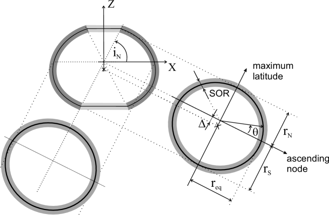
Figure 1: Geometric relation between the SOV/SOR/SOA and the frozen orbit trajectory (southward offset and flattening have been exaggerated for clarity)

Minimum Space Occupancy (MiSO) Orbits

Let us now consider a much more realistic orbit dynamics model that includes tesseral harmonics, lunisolar third-body perturbations, solar radiation pressure, and atmospheric drag. For the results obtained in this article, the solar radiation pressure perturbation is computed employing a cannonball model with a reflectivity coefficient $C_{R}=1.2$ and an area to mass ratio of $0.01\>\mathrm{m}^{2}/\mathrm{kg}$, atmospheric drag is calculated with the same area-to-mass ratio, a drag coefficient $C_{D}=2.2$, and a simplified static atmospheric model taken from Vallado [14, page 564]. The position of Sun and Moon have been computed using JPL ephemerides. Finally, we have considered a $23\times 23$ geopotential model with tesseral harmonic coefficients taken from the GRIM5-S1 model [15].

It is clear that zero-occupancy, perfectly frozen orbits cease to exist in this perturbation environment. The fundamental question is then how small space occupancy can be made by choosing optimized initial conditions leading to what we call here minimum space occupancy (MiSO) orbits. The answer to this question can have profound implications on the design of future mega-constellation of satellites, which could be organized by stacking non-overlapping space occupancy regions corresponding to each orbital plane one on top of another by a judicious selection of the minimum altitude of each plane.

The computation of MiSO initial conditions for the numerical cases considered in this article has been done numerically using an adaptive grid-search algorithm to converge to a minimum-occupancy solution starting from frozen-orbit conditions obtained from the previously described analytical development. It is important to underline that each individual point in the grid-search process is a high-fidelity propagation whose timespan is the one associated to the current SOR definition (i.e. 100 days) and includes an accurate computation of the SOR starting from the propagated state vector. This is a very demanding process in terms of CPU time (the computation of MiSO initial conditions for an individual constellation plane can take a few hours with an Intel Core processor i7-4790@3.6GHz) where the use of a very efficient orbit propagator is paramount. All numerical propagations were performed using the THALASSA orbit propagator [16], [17].

All MiSO orbits initial conditions derived in this work are reported in Appendix II for reproducibility purposes.

Table 2: LEO orbits constellations considered in this study

orbit class	$h_{N}$ [km]	$\hat{i}$ [deg]
class 1	550	53
class 2	550	87.9
class 3	1168	53
class 4	1168	87.9
class 5	813	98.7

Five classes of nominal LEO orbits are considered (see Table 2, where $h_{N}$ denotes the altitude at maximum-latitude) in line with existing and upcoming mega-constellations and including an example of Sun-synchronous orbit (class 5). Each class comprises 12 orbits with equal mean inclination $\hat{i}$ and maximum-latitude altitude $h_{N}$ and distributed on 12 orbital planes spaced by 30 degrees in longitude of node ($\hat{\varOmega}=0^{\circ},30^{\circ},60^{\circ},...,330^{\circ})$. In other words, each class corresponds to a $"p=12"$ delta-pattern constellation (see [18]) except that the number of satellites in each orbital plane is not specified here. Regarding the last point, we note that the computation of MiSO initial conditions for multiple satellites in the same plane can be done by propagating forward in time the state of one MiSO satellite by a fraction of the orbital period without expecting any significant departure from individually-computed MiSO initial conditions. All initial conditions are referred to 1 January 2020 as initial epoch.

Two main scenarios are considered: a drag-free scenario where the effect of solar radiation pressure and drag is switched off and a more realistic scenario where both effects are present.

Drag-free MiSO orbits

Table 3 displays the drag-free, 100-day SOR for 12 orbital planes of the five classes of MiSO orbits considered in Table 2. The results clearly show that lower altitudes and near polar inclinations (i.e. class 2) results in a wider space occupancy range. This is mainly due to the combined effect of tesseral harmonics. The corresponding figures for unoptimized frozen orbits (i.e. orbits obtained by applying Eqs. (7-11)) are reported in Table 4 for comparison and show that MiSO orbits can provide an SOR reduction of up to almost 600 m compared to the unoptimized case.

Table 3: 100-day SOR [km] of MiSO orbits in drag-free conditions

orbit class	$0^{\circ}$	$30^{\circ}$	$60^{\circ}$	$90^{\circ}$	$120^{\circ}$	$150^{\circ}$	$180^{\circ}$	$210^{\circ}$	$240^{\circ}$	$270^{\circ}$	$300^{\circ}$	$330^{\circ}$
class 1	503	493	493	497	498	511	512	513	517	512	508	511
class 2	604	673	604	605	625	643	645	650	647	625	598	687
class 3	378	384	389	392	393	404	404	408	397	387	387	381
class 4	296	297	300	298	290	299	308	309	301	295	295	291
class 5	441	425	462	466	461	471	469	461	448	447	473	445

Table 4: 100-day SOR [km] of unoptimized frozen orbits in drag-free conditions

orbit class	$0^{\circ}$	$30^{\circ}$	$60^{\circ}$	$90^{\circ}$	$120^{\circ}$	$150^{\circ}$	$180^{\circ}$	$210^{\circ}$	$240^{\circ}$	$270^{\circ}$	$300^{\circ}$	$330^{\circ}$
class 1	575	658	726	754	747	603	631	901	700	860	775	801
class 2	889	1183	1040	1114	983	781	818	868	933	887	906	1272
class 3	460	505	539	549	560	484	477	603	539	637	578	584
class 4	495	434	520	470	453	426	354	570	482	337	467	586
class 5	535	508	847	876	693	664	668	536	613	771	812	776

Figures (2)-(6) show the evolution of the 10-day fixed-timespan SOR function over a period of 100 days for the 12 planes of the five classes of orbits. The size of the space occupancy region appears to fluctuate without experiencing any significant secular increase, which implies that the different gravitational perturbations do not have a significant long-term deteriorating effect on drag-free MiSO orbits.

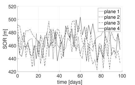
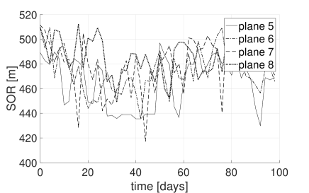
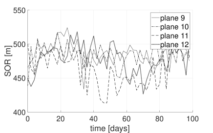
Figure 2: SOR evolution for class 1 MiSO orbits in drag-free conditions

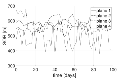
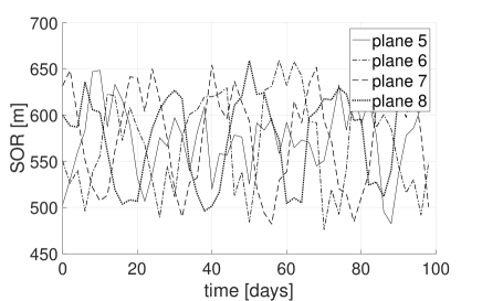
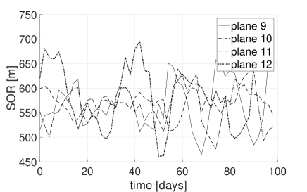
Figure 3: SOR evolution for class 2 MiSO orbits in drag-free conditions

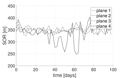
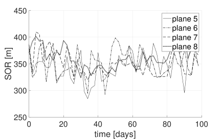
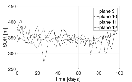
Figure 4: SOR evolution for class 3 MiSO orbits in drag-free conditions

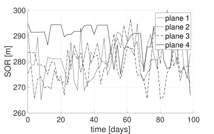
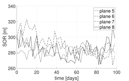
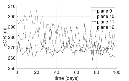
Figure 5: SOR evolution for class 4 MiSO orbits in drag-free conditions

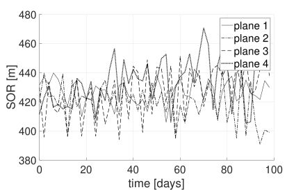
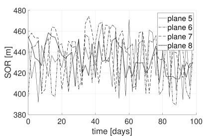
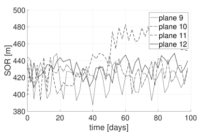
Figure 6: SOR evolution for class 5 MiSO orbits in drag-free conditions

To conclude the analysis we plot the variation of the minimum altitude in time for the different orbital planes. Such variation, measured with respect to initial minimum altitude (i.e. computed during the first 10 days), is displayed in Figures (7)-(9), where the minimum altitude function is computed in a similar way as the fixed-timespan SOR (i.e. over a moving 10-day time interval). Altitude fluctuations are contained below 50 meters for all cases with the exception of class 2, which experiences 100-m-wide altitude fluctuations in two of its planes, and class 3, which experiences a 80-m-wide altitude fluctuations in one of its planes.

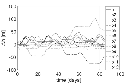
Figure 7: Evolution of the minimum altitude for all orbital planes of class 1 (left) and class 2 (right) MiSO orbits

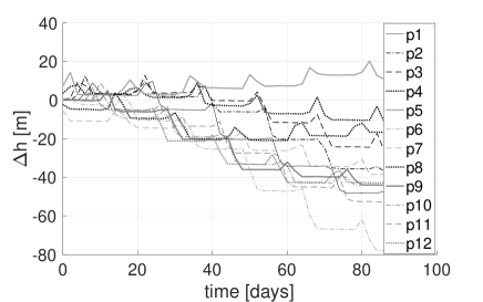
Figure 8: Evolution of minimum altitude for all orbital planes of class 3 (left) and class 4 (right) MiSO orbits

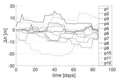
Figure 9: Evolution of minimum altitude for all orbital planes of class 5 MiSO orbits

Impact of SRP and drag

As one can expect from the available frozen-orbit literature (see in particular Shapiro [19]), solar radiation pressure and drag have a major impact on the minimum achievable space occupancy and its evolution. Even if the effect of these perturbations can be compensated by correction maneuvers it is extremely important to be able to delay the need to perform such maneuvers as much as possible by including these perturbations in the MiSO orbit design process. As an example, correction maneuvers for the frozen-orbit based Sentinel-3 mission can be as frequent as every two weeks [20].

Table 5 displays the 100-day SOR for 12 orbital planes of the five classes of MiSO orbits previously considered but with both atmospheric drag and solar radiation pressure active. The corresponding results for unoptimized frozen orbits are reported in Table 6 showing the benefit of MiSO orbits in terms of SOR reduction (up to almost 400 m). As expected, the minimum space occupancy of lower altitude orbits (class 1,2) is considerably higher compared to their drag-free counterpart mainly because of drag-induced altitude decay. For higher-altitude orbits (class 3,4,5) non-gravitational perturbations (mainly SRP) also result in an increased SOR, but to a much lesser extent. We must stress here the importance of including both types of perturbations in the process of MiSO initial conditions generation as adopting initial conditions of a drag-free MiSO orbit would result in a much bigger SOR in this scenario.

Figures (10)-(14) plot the 100-day SOR for the 12 orbital planes of the five classes of orbits while the evolution of the minimum altitude variation in time for the different orbital planes of each orbit class is displayed in Figures (15)-(17).

What clearly emerges from these plots is that the action of both types of non-gravitational perturbations tends to shift the mean altitude of the whole space occupancy region without significantly changing its size. In other words, both perturbations do not appear to be able to disrupt the frozen-like character of these orbits, at least over the 100 days time-scale considered here. This is a considerable merit of the MiSO orbit design concept. Regarding the specific influence of SRP it appears to have a stronger influence on the SOR of Sun-synchronous (class 5, Figure 14) and lower inclination orbits (class 3 rather than 4, as it is evident in Figure 12 and 13) although for the case of lower altitude orbits this tends to be masked by the dominant effect of atmospheric drag (Figure 10).

Regarding the time evolution of the minimum altitude, lower altitude MiSO orbits (Figure 15) tend to exhibit a uniform secular decay superposed to an oscillating behavior while for higher altitude the behavior is predominantly oscillatory (Figure 16,17).

A possible design strategy for a mega-constellations with non-overlapping $P$ planes is the following. After sorting the different constellation planes by ascending minimum altitude (over the desired time-span, e.g., 100 days) the nominal maximum-latitude altitude of each plane can be set to:

$$h_{N,p+1}=h_{N,p}+\mathrm{SOR_{\mathrm{\mathit{p}}}}\qquad p=0..P.$$

In the preceding equation, $\mathrm{SOR_{\mathrm{\mathit{p}}}}$ is the space occupancy range of the $P-$plane orbit accumulated over the total time-span and does take into account altitude oscillations.

This design process can be refined iteratively by recomputing the new SOR of each plane after the addition of the required altitude offset. The effectiveness of this approach has been demonstrated in a recent paper currently under review [21].

Table 5: 100-day SOR [km] of MiSO orbits including non-gravitational perturbations

orbit class	$0^{\circ}$	$30^{\circ}$	$60^{\circ}$	$90^{\circ}$	$120^{\circ}$	$150^{\circ}$	$180^{\circ}$	$210^{\circ}$	$240^{\circ}$	$270^{\circ}$	$300^{\circ}$	$330^{\circ}$
class 1	2997	3134	2952	3073	2958	3056	3072	3049	3004	2933	2956	2996
class 2	2894	3210	3049	2983	2966	3100	3034	3239	3036	2925	3022	3183
class 3	525	539	600	616	669	659	650	640	576	522	512	515
class 4	474	452	404	436	502	541	563	537	472	400	432	463
class 5	542	609	687	814	746	679	602	532	611	766	797	674

Table 6: 100-day SOR [km] of unoptimized frozen orbits including non-gravitational perturbations

orbit class	$0^{\circ}$	$30^{\circ}$	$60^{\circ}$	$90^{\circ}$	$120^{\circ}$	$150^{\circ}$	$180^{\circ}$	$210^{\circ}$	$240^{\circ}$	$270^{\circ}$	$300^{\circ}$	$330^{\circ}$
class 1	3143	3186	3166	3180	3156	3109	3210	3335	3206	3174	3178	3291
class 2	3275	3622	3148	3454	3207	3356	3270	3337	3286	3108	3515	3692
class 3	673	707	711	732	764	908	1002	1009	632	649	682	593
class 4	677	575	718	658	558	704	867	883	837	676	718	799
class 5	592	754	1063	1186	1055	1019	946	533	808	1102	1132	1011

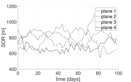
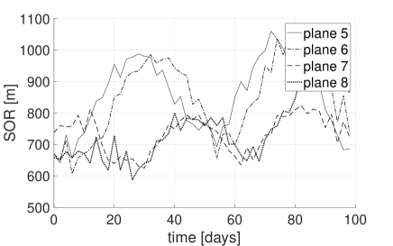
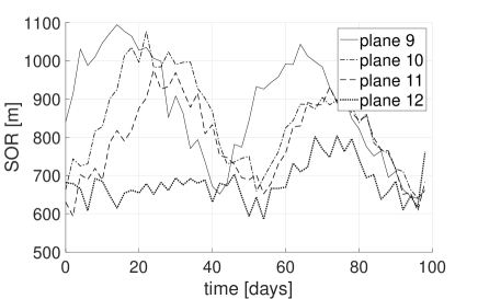
Figure 10: SOR evolution for class 1 MiSO orbits considering non-gravitational perturbations

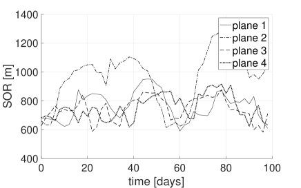
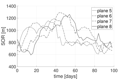
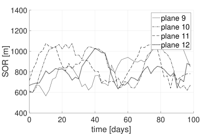
Figure 11: SOR evolution for class 2 MiSO orbits considering non-gravitational perturbations

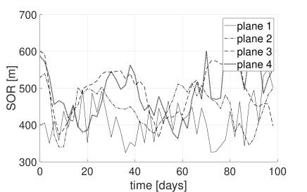
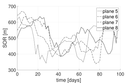
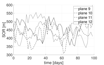
Figure 12: SOR evolution for class 3 MiSO orbits considering non-gravitational perturbations

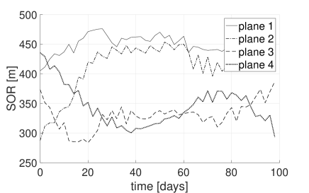
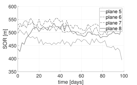
Figure 13: SOR evolution for class 4 MiSO orbits considering non-gravitational perturbations

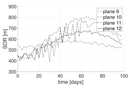
Figure 14: SOR evolution for class 5 MiSO orbits considering non-gravitational perturbations

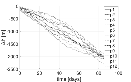
Figure 15: Evolution of the minimum altitude for all orbital planes of class 1 (left) and class 2 (right) MiSO orbits

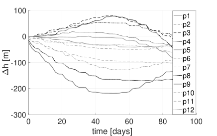
Figure 16: Evolution of minimum altitude for all orbital planes of class 3 (left) and class 4 (right) MiSO orbits

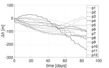
Figure 17: Evolution of minimum altitude for all orbital planes of class 5 MiSO orbits

Conclusions

The concept of space occupancy and minimum space occupancy (MiSO) orbits are promising tools to quantify and mitigate the risk of space debris accumulation in LEO as well as to minimize the frequency of collision avoidance maneuvers, especially in light of upcoming LEO mega-constellations of satellites. MiSO orbits can be seen as a generalization of frozen orbits beyond the zonal problem, where tesseral harmonics, third-body effects, and non-gravitational perturbations make it impossible to achieve constant altitude at equal latitude, i.e. “zero occupancy” conditions. In the zonal problem, frozen orbits can be conveniently characterized in osculating element space leading to a newly derived frozen orbit polar equation and providing a first guess solution for the computation of MiSO orbits when additional perturbations are included. We have numerically obtained initial conditions leading to MiSO orbits in five different scenarios in LEO and studied their behavior in time. For higher altitude orbits ($h\sim$1200 km), and with a standard area-to-mass ratio, a SOR of less than 700 m over 100 days is achievable and can be reduced below 600 m for near polar orbits (thanks to a reduced negative influence of SRP). A slightly higher SOR, 814 m in the worst case, was obtained for Sun-synchronous MiSO orbits. Lower altitude orbits ($h\sim$500 km) are characterized by a wider SOR (around 3 km in 100 days for the cases considered in this article) mainly due to atmospheric drag decay (clearly inflating the space occupancy region inwards), but also due to a stronger tesseral harmonics effect. In all cases, non-gravitational perturbations have a detrimental effect on the size of the space occupancy region but do not appear to be capable of completely disrupting the frozen-like character of the orbit, at least over a timescale of several months. It is important to add that we did not perform a detailed investigation of the behavior of MiSO orbits near to the critical inclination where bifurcations between orbit families and instability arise[22]; we leave this task for a future study.

These results suggest that the lay-out of large constellations of satellites could be effectively optimized by having all satellites flying in MiSO orbits and with an incremental stacking of non-intersecting constellation planes. The effectiveness of this solution will be further investigated.

Appendix I: Kozai-Lyddane Conversion Formulas

Following Kozai [12] (or equivalently, Brouwer [11]) , the ($J_{2}$-dominated) short-periodic terms for the orbital elements of the zonal problem, after indicating with $\hat{}$ the mean ( = secular + long-periodic) component of each element, are as follows:

semi-major axis:

$$a_{sp}=\dfrac{J_{2}}{2\hat{a}}\left[\left(2-3\kappa\right)\left(\dfrac{\hat{a}^{3}}{\hat{r}^{3}}-\dfrac{1}{\eta^{3}}\right)+\dfrac{3\kappa\hat{a}^{3}}{\hat{r}^{3}}\,c_{2,2}\right].$$ (15)

eccentricity:

$$\begin{array}[]{c}e_{sp}=\dfrac{3J_{2}\lambda^{2}}{4\hat{e}\hat{a}^{2}}\left[\left(2-3\kappa\right)\left(\dfrac{\hat{a}^{3}}{\hat{r}^{3}}-\dfrac{1}{\lambda^{3}}\right)+\dfrac{3\kappa\hat{a}^{3}}{\hat{r}^{3}}\,c_{2,2}\right]\\ \\ -\dfrac{3J_{2}\kappa}{4\hat{e}\hat{a}^{2}\lambda^{2}}\left[c_{2,2}+\hat{e}c_{1,2}+\dfrac{\hat{e}}{3}c_{3,2}\right]-\dfrac{J_{2}\kappa\hat{e}\left(2\lambda+1\right)\cos\left(2\hat{\omega}\right)}{4\hat{a}^{2}\lambda^{2}\left(\lambda+1\right)^{2}}.\end{array}$$ (16)

inclination:

$$\begin{array}[]{c}\begin{array}[]{c}i_{sp}=\dfrac{J_{2}}{8\hat{a}^{2}\lambda^{4}}\sin 2\hat{i}\left[3c_{2,2}+3\hat{e}c_{1,2}+\hat{e}c_{3,2}\right]\end{array}\\ \\ -\dfrac{J_{2}\sin 2\hat{i}\left(2\lambda^{2}-\lambda-1\right)\cos\left(2\hat{\omega}\right)}{8\hat{a}^{2}\lambda^{2}\left(\lambda+1\right)}.\end{array}$$ (17)

longitude of the ascending node:

$$\begin{array}[]{c}\begin{array}[]{c}\Omega_{sp}=-\dfrac{3J_{2}\sqrt{1-\kappa}}{2a^{2}\lambda^{4}}\left[\hat{\nu}-\hat{M}+\hat{e}\,s_{1,0}-\dfrac{1}{2}\left(s_{2,2}+\hat{e}\,s_{1,2}+\dfrac{\hat{e}\,s_{3,2}}{3}\right)\right]\end{array}\\ \\ -\dfrac{J_{2}\sqrt{1-\kappa}\left(2\lambda^{2}-\lambda-1\right)\sin\left(2\hat{\omega}\right)}{4\hat{a}^{2}\lambda^{4}\left(\lambda+1\right)}.\end{array}$$ (18)

argument of pericenter:

$$\begin{array}[]{c}\omega_{sp}=\dfrac{3J_{2}}{2\hat{a}^{2}\lambda^{4}}\left\{\dfrac{4-5\kappa}{2}\left(\hat{\nu}-\hat{M}+\hat{e}\,s_{1,0}\right)+\dfrac{5\kappa-2}{4}\left(s_{2,2}+\hat{e}s_{1,2}+\dfrac{\hat{e}}{3}s_{3,2}\right)\right.\\ \\ +\dfrac{\lambda^{2}}{\hat{e}}\left(\dfrac{2-3\kappa}{2}\left[\left(1-\dfrac{\hat{e}^{2}}{4}\right)s_{1,0}+\dfrac{\hat{e}}{2}s_{2,0}+\dfrac{\hat{e}^{2}}{12}s_{3,0}\right]\right.\\ \\ +\kappa\left[\dfrac{1}{4}\left(1+\dfrac{5}{4}\hat{e}^{2}\right)s_{1,2}-\dfrac{\hat{e}^{2}}{16}s_{1,-2}\right.\\ \\ \left.\left.\left.-\dfrac{7}{12}\left(1-\dfrac{\hat{e}^{2}}{28}\right)s_{3,2}-\dfrac{3}{8}\hat{e}s_{4,2}-\dfrac{\hat{e}^{2}}{16}s_{5,2}\right]\right)\right\}\\ \\ +\dfrac{3J_{2}\sqrt{1-\kappa}}{2\hat{a}^{2}\lambda^{4}}\left[\dfrac{\kappa}{8}+\dfrac{\left(1+2\lambda\right)\left(2\kappa\lambda^{2}-\lambda^{2}-\kappa+1\right)}{6\left(\lambda+1\right)^{2}}\right]\sin\left(2\hat{\omega}\right).\end{array}$$ (19)

mean anomaly:

$$\begin{array}[]{c}\hat{e}M_{sp}=-\dfrac{3J_{2}}{2\hat{a}^{2}\lambda^{3}}\left\{\dfrac{2-3\kappa}{2}\left[\left(1-\dfrac{\hat{e}^{2}}{4}\right)s_{1,0}+\dfrac{\hat{e}}{2}s_{2,0}+\dfrac{\hat{e}^{2}}{12}s_{3,0}\right]\right.\\ \\ -\kappa\left[\dfrac{1}{4}\left(1+\dfrac{5}{4}\hat{e}^{2}\right)s_{1,2}-\dfrac{\hat{e}^{2}}{16}s_{1,-2}\right.\\ \\ \left.\left.-\dfrac{7}{12}\left(1-\dfrac{\hat{e}^{2}}{28}\right)s_{3,2}-\dfrac{3}{8}\hat{e}s_{4,2}-\dfrac{\hat{e}^{2}}{16}s_{5,2}\right]\right\}\\ \\ +\hat{e}\dfrac{J_{2}\kappa\left(4\lambda^{3}-\lambda^{2}-18\lambda-9\right)\sin\left(2\hat{\omega}\right)}{16\hat{a}^{2}\lambda^{3}\left(\lambda+1\right)^{2}},\end{array}$$ (20)

with:

$$\lambda=\sqrt{1-\hat{e}^{2}},\qquad\kappa=\sin^{2}\hat{i},$$

$$\hat{r}=\frac{\hat{a}\left(1-\hat{e}^{2}\right)}{1+\hat{e}\cos\hat{\nu}},$$

$$s_{1,0}=\sin\hat{\nu},\qquad s_{2,0}=\sin 2\hat{\nu},\qquad s_{3,0}=\sin 3\hat{\nu},$$

$$s_{1,2}=\sin\left(\hat{\nu}+2\hat{\omega}\right),\qquad s_{1,-2}=\sin\left(\hat{\nu}-2\hat{\omega}\right),\qquad s_{2,2}=\sin\left(2\hat{\nu}+2\hat{\omega}\right),$$

$$s_{3,2}=\sin\left(3\hat{\nu}+2\hat{\omega}\right),\qquad s_{4,2}=\sin\left(4\hat{\nu}+2\hat{\omega}\right),\qquad s_{5,2}=\sin\left(5\hat{\nu}+2\hat{\omega}\right),$$

$$c_{1,0}=\cos\hat{\nu},\qquad c_{1,1}=\cos\left(\hat{\nu}+\hat{\omega}\right),\qquad c_{1,2}=\cos\left(\hat{\nu}+2\hat{\omega}\right),$$

$$c_{2,2}=\cos\left(2\hat{\nu}+2\hat{\omega}\right),\qquad c_{3,2}=\cos\left(3\hat{\nu}+2\hat{\omega}\right).$$

With the exception of the semi-major axis, all above expressions may become numerically unstable near circular and/or equatorial conditions. Following

Lyddane’s method [13], a numerically stable expression for the mean anomaly short-periodic can be obtained based on the expansion:

$$\left(\hat{e}+e_{sp}\right)\cos\left(\hat{M}+M_{sp}\right)\simeq\left(\hat{e}+e_{sp}\right)\cos\hat{M}-\hat{e}M_{sp}\sin\hat{M}=\varsigma,$$ (21)

$$\left(\hat{e}+e_{sp}\right)\sin\left(\hat{M}+M_{sp}\right)\simeq\left(\hat{e}+e_{sp}\right)\sin\hat{M}+\hat{e}M_{sp}\sin\hat{M}=\iota,$$ (22)

providing numerically stable expressions (denoted with a tilde) for the mean anomaly and eccentricity short-periodic components as:

$$\tilde{M}_{sp}\simeq\mathrm{atan2}\left(\iota,\varsigma\right)-\hat{M},$$ (23)

$$\tilde{e}_{sp}=\sqrt{\iota^{2}+\varsigma^{2}}-\hat{e}.$$ (24)

Similarly, using Lyddane’s expansion:

$$\sin\left(\frac{\hat{i}+i_{sp}}{2}\right)\cos\left(\hat{\Omega}+\Omega_{sp}\right)\simeq\left(\sin\frac{\hat{i}}{2}+\frac{i_{sp}}{2}\cos\frac{\hat{i}}{2}\right)\cos\hat{\Omega}-\sin\frac{\hat{i}}{2}\sin\hat{\Omega}\,\Omega_{sp}=\varrho,$$

$$\sin\left(\frac{\hat{i}+i_{sp}}{2}\right)\sin\left(\hat{\Omega}+\Omega_{sp}\right)\simeq\left(\sin\frac{\hat{i}}{2}+\frac{i_{sp}}{2}\cos\frac{\hat{i}}{2}\right)\sin\hat{\Omega}+\sin\frac{\hat{i}}{2}\cos\hat{\Omega}\,\Omega_{sp}=\kappa,$$

stable expressions for the right ascension of the ascending node and the inclination are obtained:

$$\tilde{\Omega}_{sp}\simeq\mathrm{atan2}\left(\kappa,\varrho\right)-\hat{\Omega},$$ (25)

$$\tilde{i}_{sp}=2\sin^{-\text{1}}\sqrt{\left(\varrho^{2}+\kappa^{2}\right)}.$$ (26)

The non-singular expression for the argument of periapsis short-periodic component can be computed as:

$$\tilde{\omega}_{sp}=\ell_{sp}-\tilde{M}_{sp}-\tilde{\Omega}_{sp}.$$ (27)

where:

$$\ell_{sp}=M_{sp}+\omega_{sp}+\Omega_{sp}$$

is the short-periodic component of the mean longitude and reads (from Eqs. (18-20)):

$$\begin{array}[]{c}\ell_{sp}=\dfrac{3J_{2}}{2\hat{a}^{2}\lambda^{4}}\left\{\left(\dfrac{4-5\kappa}{2}-\sqrt{1-\kappa}\right)\left(\hat{\nu}-\hat{M}+\hat{e}\,s_{1,0}\right)\right.\\ \\ +\left(\dfrac{5\kappa-2}{4}+\dfrac{\sqrt{1-\kappa}}{2}\right)\left(s_{2,2}+es_{1,2}+\dfrac{\hat{e}}{3}s_{3,2}\right)\\ \\ +\dfrac{\hat{e}}{1+\lambda}\left(\dfrac{2-3\kappa}{2}\left[\left(1-\dfrac{\hat{e}^{2}}{4}\right)s_{1,0}+\dfrac{\hat{e}}{2}s_{2,0}+\dfrac{\hat{e}^{2}}{12}s_{3,0}\right]\right.\\ \\ +\kappa\left[\dfrac{1}{4}\left(1+\dfrac{5}{4}\hat{e}^{2}\right)s_{1,2}-\dfrac{\hat{e}^{2}}{16}s_{1,-2}\right.\\ \\ \left.\left.\left.-\dfrac{7}{12}\left(1-\dfrac{\hat{e}^{2}}{28}\right)s_{3,2}-\dfrac{3}{8}\hat{e}s_{4,2}-\dfrac{\hat{e}^{2}}{16}s_{5,2}\right]\right)\right\}\\ \\ +\dfrac{3J_{2}\sqrt{1-\kappa}}{2\hat{a}^{2}\lambda^{4}}\left[\dfrac{\kappa}{8}+\dfrac{\left(1+2\lambda\right)\left(2\kappa\lambda^{2}-\lambda^{2}-\kappa+1\right)}{6\left(\lambda+1\right)^{2}}\right]\sin\left(2\hat{\omega}\right)\\ \\ +\dfrac{J_{2}\kappa\left(4\lambda^{3}-\lambda^{2}-18\lambda-9\right)\sin\left(2\hat{\omega}\right)}{16\hat{a}^{2}\lambda^{3}\left(\lambda+1\right)^{2}}-\dfrac{J_{2}\sqrt{1-\kappa}\left(2\lambda^{2}-\lambda-1\right)\sin\left(2\hat{\omega}\right)}{4\hat{a}^{2}\lambda^{4}\left(\lambda+1\right)}.\end{array}$$ (28)

Appendix II: MiSO orbit initial conditions

• We report the initial conditions in terms of classical orbital elements for the five classes of orbits with and without SRP and drag. The reference epoch is 1 January 2020 (JD=2458849.5).

class 1, drag-free

$$\left[\begin{array}[]{cccccc}\Omega(^{\circ})&a(\mathrm{km})&e()&inc(^{\circ})&\omega(^{\circ})&M_{0}(^{\circ})\\ 0&6932.759064&0.0003334517026&52.98106159&90.54762182&359.4527433\\ 30.0&6932.601577&0.0003222155192&52.98106159&87.73258259&2.265956955\\ 60.0&6932.584891&0.0003210841031&52.98106159&87.15531659&2.842857835\\ 90.0&6932.567921&0.0003199118596&52.98106159&86.80193533&3.196020025\\ 120.0&6932.550011&0.0003186039891&52.98106159&86.90359531&3.094433071\\ 150.0&6932.738275&0.0003320120194&52.98106159&88.37426286&1.624658026\\ 180.0&6932.829753&0.0003385453073&52.98106159&89.56849536&0.4312125478\\ 210.0&6933.077243&0.0003563831289&52.98106159&90.0&4.042782711\cdot 10^{-12}\\ 240.0&6932.583903&0.0003209417217&52.98106159&92.27641993&357.7250405\\ 270.0&6932.505325&0.0003155593633&52.98106159&94.13133918&355.8712653\\ 300.0&6932.641127&0.0003253686865&52.98106159&94.15663717&355.8460647\\ 330.0&6932.921076&0.0003453388649&52.98106159&92.85652342&357.1454482\end{array}\right]$$

class 2, drag-free

$$\left[\begin{array}[]{cccccc}\Omega(^{\circ})&a(\mathrm{km})&e()&inc(^{\circ})&\omega(^{\circ})&M_{0}(^{\circ})\\ 0&6928.137945&0.0004628998797&87.89855475&270.0&180.0\\ 30.0&6928.142547&0.0004686537004&87.89855475&266.9618906&183.0409567\\ 60.0&6928.138892&0.000454128096&87.89855475&268.5534594&181.4478548\\ 90.0&6928.14189&0.0004596507278&87.89855475&272.859197&177.1381748\\ 120.0&6928.140508&0.0004709049191&87.89855475&272.2478274&177.7500554\\ 150.0&6928.138081&0.0004832807396&87.89855475&269.9244934&180.0755796\\ 180.0&6928.138124&0.0004883770586&87.89855475&269.850563&180.149583\\ 210.0&6928.138271&0.0004667646813&87.89855475&269.2181866&180.7825434\\ 240.0&6928.139876&0.0004759041062&87.89855475&268.0827124&181.9191128\\ 270.0&6928.139195&0.0004719882596&87.89855475&268.4535424&181.5479178\\ 300.0&6928.138817&0.0004617530503&87.89855475&271.3435928&178.6551661\\ 330.0&6928.142847&0.0004577776823&87.89855475&273.1961256&176.8009487\end{array}\right]$$

class 3, drag-free

$$\left[\begin{array}[]{cccccc}\Omega(^{\circ})&a(\mathrm{km})&e()&inc(^{\circ})&\omega(^{\circ})&M_{0}(^{\circ})\\ 0&7551.070081&0.0003267389013&52.98403631&90.28264403&359.7175406\\ 30.0&7550.941064&0.0003182546944&52.98403631&88.45220381&1.546811358\\ 60.0&7550.925068&0.0003172114877&52.98403631&88.25294551&1.745946553\\ 90.0&7550.925471&0.0003172647177&52.98403631&87.96199778&2.036709626\\ 120.0&7550.942161&0.0003183997827&52.98403631&87.67901118&2.319511573\\ 150.0&7550.98916&0.0003213985795&52.98403631&89.13795204&0.8614939899\\ 180.0&7551.086314&0.0003278134345&52.98403631&90.2817177&359.718467\\ 210.0&7551.232544&0.0003375013701&52.98403631&90.63848614&359.3619447\\ 240.0&7550.860418&0.0003129504061&52.98403631&91.96767998&358.0335511\\ 270.0&7550.796865&0.0003088343336&52.98403631&92.79201685&357.2097066\\ 300.0&7550.910426&0.0003163473872&52.98403631&92.72566777&357.2760557\\ 330.0&7551.136052&0.0003311743495&52.98403631&91.67338604&358.3277219\end{array}\right]$$

class 4, drag-free

$$\left[\begin{array}[]{cccccc}\Omega(^{\circ})&a(\mathrm{km})&e()&inc(^{\circ})&\omega(^{\circ})&M_{0}(^{\circ})\\ 0&7546.137417&0.0003554791211&87.89878205&269.9134623&180.0865992\\ 30.0&7546.137812&0.0003619697371&87.89878205&269.0651164&180.9355606\\ 60.0&7546.137518&0.0003544195479&87.89878205&269.4792143&180.521155\\ 90.0&7546.13762&0.0003576521232&87.89878205&270.6881109&179.3113968\\ 120.0&7546.13854&0.0003642120497&87.89878205&271.6049943&178.3938364\\ 150.0&7546.138352&0.000372771327&87.89878205&271.4030248&178.595929\\ 180.0&7546.137523&0.0003748075505&87.89878205&269.9179258&180.0821358\\ 210.0&7546.140531&0.0003612565296&87.89878205&267.2740604&182.7279089\\ 240.0&7546.139481&0.0003686287757&87.89878205&267.8297766&182.1718234\\ 270.0&7546.137505&0.0003672941004&87.89878205&270.2512612&179.7485542\\ 300.0&7546.138211&0.0003598764869&87.89878205&271.367811&178.6312043\\ 330.0&7546.138634&0.0003534942316&87.89878205&271.7407412&178.258028\end{array}\right]$$

class 5, drag-free

$$\left[\begin{array}[]{cccccc}\Omega(^{\circ})&a(\mathrm{km})&e()&inc(^{\circ})&\omega(^{\circ})&M_{0}(^{\circ})\\ 0&7191.138473&0.0004861880768&98.7382975&270.7663379&179.2329167\\ 30.0&7191.138377&0.0004873559266&98.7382975&269.3745053&180.6261046\\ 60.0&7191.13945&0.0004662437432&98.7382975&268.3289104&181.6726482\\ 90.0&7191.141517&0.0004700743544&98.7382975&267.4051815&182.5972581\\ 120.0&7191.139764&0.000482823931&98.7382975&268.2459627&181.7557314\\ 150.0&7191.139363&0.0004993041537&98.7382975&268.5753276&181.4260955\\ 180.0&7191.138775&0.0005039469162&98.7382975&269.0590254&180.9419233\\ 210.0&7191.138153&0.0004837814401&98.7382975&269.8599766&180.140159\\ 240.0&7191.138789&0.0004803262336&98.7382975&271.1283193&178.8705965\\ 270.0&7191.142094&0.000486690954&98.7382975&272.715144&177.2822131\\ 300.0&7191.142097&0.0004843290287&98.7382975&272.7283982&177.268959\\ 330.0&7191.141897&0.000484301249&98.7382975&272.6585409&177.338884\end{array}\right]$$

class 1, with drag and SRP

$$\left[\begin{array}[]{cccccc}\Omega(^{\circ})&a(\mathrm{km})&e()&inc(^{\circ})&\omega(^{\circ})&M_{0}(^{\circ})\\ 0&6932.847704&0.0003398589364&52.98106159&89.03282984&0.966512953\\ 30.0&6932.847373&0.0003398111148&52.98106159&89.89252657&0.1074004103\\ 60.0&6932.374999&0.0003061144251&52.98106159&86.0599343&3.937655933\\ 90.0&6932.688387&0.000328359523&52.98106159&89.33265961&0.6669022514\\ 120.0&6932.373341&0.0003058754377&52.98106159&86.77463005&3.223398318\\ 150.0&6932.635623&0.0003245754356&52.98106159&88.87475421&1.124515558\\ 180.0&6933.006515&0.0003512844274&52.98106159&89.89603617&0.1038908093\\ 210.0&6933.165975&0.000362802605&52.98106159&89.09398865&0.9053541528\\ 240.0&6932.958716&0.0003482162884&52.98106159&93.77840363&356.2242252\\ 270.0&6932.850391&0.000340246043&52.98106159&92.89930889&357.1026627\\ 300.0&6932.849824&0.0003401643041&52.98106159&92.61337609&357.3884008\\ 330.0&6932.795681&0.0003361819257&52.98106159&91.95578046&358.0455339\end{array}\right]$$

class 2, with drag and SRP

$$\left[\begin{array}[]{cccccc}\Omega(^{\circ})&a(\mathrm{km})&e()&inc(^{\circ})&\omega(^{\circ})&M_{0}(^{\circ})\\ 0&6928.139579&0.000455924017&87.89855475&268.1321102&181.8695933\\ 30.0&6928.140254&0.0005039540111&87.89855475&268.0445949&181.9573763\\ 60.0&6928.138861&0.0004464878217&87.89855475&268.5286952&181.4726189\\ 90.0&6928.138877&0.000450307952&87.89855475&271.4588177&178.5398682\\ 120.0&6928.139415&0.0004961982704&87.89855475&271.5445355&178.4539314\\ 150.0&6928.138288&0.0005108813245&87.89855475&269.8095296&180.1906651\\ 180.0&6928.140232&0.0004963159694&87.89855475&271.9855173&178.0125115\\ 210.0&6928.139991&0.0004818593136&87.89855475&271.9440925&178.0540336\\ 240.0&6928.141251&0.0004671942162&87.89855475&267.4215977&182.5808115\\ 270.0&6928.13852&0.0005151562307&87.89855475&270.6375138&179.3618291\\ 300.0&6928.141947&0.0004392966006&87.89855475&272.9918218&177.0055499\\ 330.0&6928.140676&0.0004492946643&87.89855475&272.4373195&177.5604903\end{array}\right]$$

class 3, with drag and SRP

$$\left[\begin{array}[]{cccccc}\Omega(^{\circ})&a(\mathrm{km})&e()&inc(^{\circ})&\omega(^{\circ})&M_{0}(^{\circ})\\ 0&7550.845248&0.0003118971737&52.98403631&91.34898058&358.6518606\\ 30.0&7550.754644&0.0003058712851&52.98403631&90.80515351&359.1953389\\ 60.0&7550.794622&0.0003085376134&52.98403631&91.21951891&358.7812334\\ 90.0&7550.929887&0.0003174913716&52.98403631&91.19590232&358.8048568\\ 120.0&7551.133363&0.0003309378911&52.98403631&90.69249227&359.3079659\\ 150.0&7551.346447&0.0003450581501&52.98403631&91.03096422&358.969747\\ 180.0&7551.492367&0.0003547038822&52.98403631&90.75218097&359.2483525\\ 210.0&7551.549974&0.0003585090176&52.98403631&90.5247479&359.4756282\\ 240.0&7551.109944&0.00032938964&52.98403631&89.25232889&0.7471786939\\ 270.0&7550.842793&0.0003116915439&52.98403631&89.93415873&0.06580023575\\ 300.0&7550.843054&0.0003117261164&52.98403631&90.85587323&359.1446602\\ 330.0&7550.956833&0.0003192678224&52.98403631&91.0606653&358.9400118\end{array}\right]$$

class 4, with drag and SRP

$$\left[\begin{array}[]{cccccc}\Omega(^{\circ})&a(\mathrm{km})&e()&inc(^{\circ})&\omega(^{\circ})&M_{0}(^{\circ})\\ 0&7546.138016&0.0003562560579&87.79872416&271.2089743&178.7901641\\ 30.0&7546.138063&0.0003585275642&87.79872416&268.7605451&181.2403439\\ 60.0&7546.139345&0.0003497552251&87.79872416&267.7908264&182.210719\\ 90.0&7546.138529&0.0003540585378&87.79872416&268.3392998&181.6618763\\ 120.0&7546.137756&0.0003688594585&87.79872416&269.2030605&180.7975275\\ 150.0&7546.138011&0.0003804577162&87.79872416&268.9757809&181.0249987\\ 180.0&7546.139199&0.0003891986586&87.79872416&268.1115078&181.8899624\\ 210.0&7546.141828&0.0003856124813&87.79872416&266.9050342&183.0973522\\ 240.0&7546.139077&0.0003932358682&87.79872416&268.2091741&181.7922345\\ 270.0&7546.139725&0.0003836650407&87.79872416&272.2099263&177.7883779\\ 300.0&7546.142083&0.0003684783715&87.79872416&273.2948053&176.7027673\\ 330.0&7546.142174&0.0003595486915&87.79872416&273.3862663&176.6112994\end{array}\right]$$

class 5, with drag and SRP

$$\left[\begin{array}[]{cccccc}\Omega(^{\circ})&a(\mathrm{km})&e()&inc(^{\circ})&\omega(^{\circ})&M_{0}(^{\circ})\\ 0&7191.138373&0.000493261026&98.7382975&270.549335&179.4501229\\ 30.0&7191.139938&0.0004946594852&98.7382975&268.2194503&181.7823116\\ 60.0&7191.141711&0.0004712825164&98.7382975&267.3398952&182.6626121\\ 90.0&7191.141996&0.0004768634963&98.7382975&267.2674714&182.7351346\\ 120.0&7191.142092&0.0004890529023&98.7382975&267.2979821&182.7046608\\ 150.0&7191.141703&0.0005043534467&98.7382975&267.5144753&182.488032\\ 180.0&7191.140867&0.0005148671179&98.7382975&267.8944508&182.1077177\\ 210.0&7191.138209&0.0004922321172&98.7382975&269.8904146&180.1096933\\ 240.0&7191.140188&0.0004864262899&98.7382975&271.9500414&178.0480612\\ 270.0&7191.142089&0.0004925958671&98.7382975&272.6825648&177.3147924\\ 300.0&7191.142092&0.0004890529023&98.7382975&272.7020179&177.2953392\\ 330.0&7191.142092&0.0004890529023&98.7382975&272.7020179&177.2953392\end{array}\right]$$

References

• [1] B. B. Virgili, J. Dolado, H. Lewis, J. Radtke, H. Krag, B. Revelin, C. Cazaux, C. Colombo, R. Crowther, and M. Metz, “Risk to space sustainability from large constellations of satellites,” Acta Astronautica, Vol. 126, 2016, pp. 154–162, 10.1016/j.actaastro.2016.03.034.
• [2] J. Radtke, C. Kebschull, and E. Stoll, “Interactions of the space debris environment with mega constellations—Using the example of the OneWeb constellation,” Acta Astronautica, Vol. 131, 2017, pp. 55–68, 10.1016/j.actaastro.2016.11.021.
• [3] S. Le May, S. Gehly, B. Carter, and S. Flegel, “Space debris collision probability analysis for proposed global broadband constellations,” Acta Astronautica, Vol. 151, 2018, pp. 445–455, 10.1016/j.actaastro.2018.06.036.
• [4] M. Aorpimai and P. Palmer, “Analysis of frozen conditions and optimal frozen orbit insertion,” Journal of guidance, control, and dynamics, Vol. 26, No. 5, 2003, pp. 786–793, 10.2514/2.5113.
• [5] R. Bhat, B. Shapiro, R. Frauenholz, and R. Leavitt, “TOPEX/Poseidon orbit maintenance for the first five years (AAS 98-379),” 13th International Symposium on Space Flight Dynamics, NASA/CP-1998-206858, Vol. 2, American Astronautical Society, 1998, pp. 953–968.
• [6] T. Nie and P. Gurfil, “Lunar frozen orbits revisited,” Celestial Mechanics and Dynamical Astronomy, Vol. 130, No. 10, 2018, p. 61, 10.1007/s10569-018-9858-0.
• [7] A. Abad, A. Elipe, and E. Tresaco, “Analytical model to find frozen orbits for a lunar orbiter,” Journal of guidance, control, and dynamics, Vol. 32, No. 3, 2009, pp. 888–898, 10.2514/1.38350.
• [8] E. Condoleo, M. Cinelli, E. Ortore, and C. Circi, “Frozen orbits with equatorial perturbing bodies: the case of Ganymede, Callisto, and Titan,” Journal of Guidance, Control, and Dynamics, Vol. 39, No. 10, 2016, pp. 2264–2272, 10.2514/1.G000455.
• [9] E. Tresaco, A. Elipe, and J. P. S. Carvalho, “Frozen orbits for a solar sail around Mercury,” Journal of Guidance, Control, and Dynamics, Vol. 39, No. 7, 2016, pp. 1659–1666, 10.2514/1.G001510.
• [10] G. Cook, “Perturbations of near-circular orbits by the earth’s gravitational potential,” Planetary and Space Science, Vol. 14, No. 5, 1966, pp. 433 – 444, 10.1016/0032-0633(66)90015-8.
• [11] D. Brouwer, “Solution of the problem of artificial satellite theory without drag,” The Astronomical Journal, Vol. 64, Nov. 1959, pp. 378–397, 10.1086/107958.
• [12] Y. Kozai, “The motion of a close earth satellite,” The Astronomical Journal, Vol. 64, Nov. 1959, pp. 367–377, 10.1086/107957.
• [13] R. H. Lyddane, “Small eccentricities or inclinations in the Brouwer theory of the artificial satellite,” The Astronomical Journal, Vol. 68, Oct. 1963, pp. 555–558, 10.1086/109179.
• [14] D. A. Vallado, Fundamentals of astrodynamics and applications. Berlin: Springer, ISBN: 978-0-387-71831-6, 2007, pp. 563-564.
• [15] R. Biancale, G. Balmino, J.-M. Lemoine, J.-C. Marty, B. Moynot, F. Barlier, P. Exertier, O. Laurain, P. Gegout, P. Schwintzer, C. Reigber, A. Bode, R. König, F.-H. Massmann, J.-C. Raimondo, R. Schmidt, and S. Yuan Zhu, “A new global Earth’s gravity field model from satellite orbit perturbations: GRIM5-S1,” Geophysical Research Letters, Vol. 27, Nov. 2000, pp. 3611–3614, 10.1029/2000GL011721.
• [16] D. Amato, C. Bombardelli, G. Baù, V. Morand, and A. J. Rosengren, “Non-averaged regularized formulations as an alternative to semi-analytical orbit propagation methods,” Celestial Mechanics and Dynamical Astronomy, Vol. 131, May 2019, pp. 1–38, 10.1007/s10569-019-9897-1.
• [17] D. Amato, A. J. Rosengren, and C. Bombardelli, “THALASSA: a fast orbit propagator for near-Earth and cislunar space,” 2018 Space Flight Mechanics Meeting, 2018, p. 1970, 10.2514/6.2018-1970.
• [18] J. Walker, “Some circular orbit patterns providing continuous whole earth coverage,” Journal of the British Interplanetary Society, Vol. 24, 1971, pp. 369–384.
• [19] B. E. Shapiro, “Phase plane analysis and observed frozen orbit for the Topex/Poseidon mission,” Sixth International Space Conference of Pacific-Basin Societies, AAS Advances Series, Vol. 91, 1995, pp. 1–20.
• [20] D. A. Taboada, J. M. De Juana Gamo, P. L. Righetti, et al., “Sentinel-3 orbit control strategy,” AIAC18: 18th Australian International Aerospace Congress (2019): HUMS-11th Defence Science and Technology (DST) International Conference on Health and Usage Monitoring (HUMS 2019): ISSFD-27th International Symposium on Space Flight Dynamics (ISSFD), Melbourne: Engineers Australia, Royal Aeronautical Society, ISBN: 9781925627213, 2019, pp. 1327–1337.
• [21] N. Reiland, A. J. Rosengren, R. Malhotra, and C. Bombardelli, “Assessing and Minimizing Collisions in Satellite Mega-Constellations,” arXiv preprint arXiv:2002.00430, 2020.
• [22] S. L. Coffey, A. Deprit, and B. R. Miller, “The critical inclination in artificial satellite theory,” Celestial mechanics, Vol. 39, No. 4, 1986, pp. 365–406, 10.1007/BF01230483.