Disentangling observable dependence in SCET_I and SCET_II anomalous dimensions: angularities at two loops

Abstract

The resummation of radiative corrections to collider jet observables using soft collinear effective theory is encoded in differential renormalization group equations (RGEs), with anomalous dimensions depending on the observable under consideration. This observable dependence arises from the ultraviolet (UV) singular structure of real phase space integrals in the effective field theory. We show that the observable dependence of anomalous dimensions in SCET_I problems can be disentangled by introducing a suitable UV regulator in real radiation integrals. Resummation in the presence of the new regulator can be performed by solving a two-dimensional system of RGEs in the collinear and soft sectors, and resembles many features of resummation in SCET_II theories by means of the rapidity renormalization group. We study the properties of SCET_I with the additional regulator and explore the connection with the system of RGEs in SCET_II theories, highlighting some universal patterns that can be exploited in perturbative calculations. As an application, we compute the two-loop soft and jet anomalous dimensions for a family of recoil-free angularities and give new analytic results. This allows us to study the relations between the SCET_I and SCET_II limits for these observables. We also discuss how the extra UV regulator can be exploited to calculate anomalous dimensions numerically, and the prospects for numerical resummation.

1 Introduction

The resummation of radiative corrections in the framework of soft collinear effective theory (SCET) Bauer:2000ew ; Bauer:2000yr ; Bauer:2001ct ; Bauer:2001yt is achieved by integrating renormalization group equations (RGEs) in the effective theory. The anomalous dimensions governing such RGEs depend on the observable under consideration. In the resummation of jet collider observables, this observable dependence is related to the presence of ultraviolet (UV) divergences in real radiation integrals of the effective theory originating from the expansion of the physical phase space using power counting dictated by the SCET Lagrangian. At the same time some elements of the anomalous dimensions, those arising from virtual UV divergences are universal across observables for a given physical process. An interesting question is whether such observable dependent and independent components can be understood and disentangled, hence unveiling some common patterns and consistency relations that can be exploited when performing perturbative calculations.

We limit ourselves to collider jet observables in SCET_I and SCET_II. In SCET_II problems, the UV singularities of the phase space integrals can be handled with the rapidity renormalization group Chiu:2011qc ; Chiu:2012ir , which encodes the full observable dependence in the rapidity anomalous dimension. An alternative approach to this problem was originally formulated in Refs. Becher:2010tm ; Becher:2011pf . In SCET_I problems this separation does not occur as both UV and IR divergences are regulated by pure dimensional regularization.

To be concrete, we consider the toy example of generalized angularities in electron-positron collisions (an analogous jet-based observable was defined in Ref. Larkoski:2014pca )

$$\tau=\sum_{i}\left(\frac{k_{i,\perp}}{Q}\right)^{\alpha}e^{-\beta|\eta_{i}|}\,,$$ (1)

where the transverse momentum $k_{i,\perp}$ and pseudorapidity $\eta_{i}$ are taken with respect to the recoil-free winner-take-all axis, and $Q$ is the center-of-mass energy of the collision. Note that, if the sum runs over (massless) partons in the event, this observable is only collinear safe for $\alpha=1$ (with $\beta>-\alpha$ to ensure IR safety). This is the case of conventional angularities Berger:2003iw for which one has $\alpha=1$ and $\beta=1-a$; the case $a=0$ ($\beta=1$) corresponds to a thrust-like angularity (denoted by thrust in the rest of the paper), while $a=1$ ($\beta=0$) corresponds to a recoil-free version of jet broadening. For $\alpha\neq 1$, an alternative collinear safe version of the observable (1) with the same scaling behavior as in Eq. (2) can, for instance, be defined as in Ref. Dasgupta:2020fwr by using Lund Jet Plane Dreyer:2018nbf clusters rather partons. Alternatively, one can adopt a track based definition as in Ref. Larkoski:2014pca . All explicit computations in this article will refer to the simple case of Eq. (1) of $\alpha=1$ with the sum running over massless partons. However, since many of the considerations made in the paper only depend on the scaling (2), we will keep the dependence on $\alpha$ in the rest of the paper. While any explicit results given in the paper that refer to the factorization theorem (3) only hold for $\alpha=1$, by keeping the general dependence on $\alpha$ and $\beta$ we make our results easily extendable to other observables, albeit with different factorization theorems.

In the limit $\tau\to 0$, the logarithms of $\tau$ can be resummed to all orders in perturbation theory Berger:2003iw ; Bauer:2008dt ; Hornig:2009vb ; Larkoski:2014uqa ; Banfi:2018mcq ; Bell:2018gce ; Procura:2018zpn (see also Ref. Kang:2018vgn for groomed angularities at hadron colliders). In SCET_I ($\beta\neq 0$), this resummation is accomplished by observing that the problem contains three separate mass scales, a hard, jet and soft scale

$$M_{H} =Q\,, M_{J} =Q\,\tau^{1/(\alpha+\beta)}\,, M_{S} =Q\,\tau^{1/\alpha}\,,$$ (2)

and the differential cross section can be expressed by means of the following factorization theorem valid for the recoil-free case at leading power Larkoski:2014uqa

$$\frac{1}{\sigma_{\rm Born}}\frac{{\rm d}\sigma}{{\rm d}\tau}=H(M_{H},\mu)\int{\rm d}\tau_{n}\,{\rm d}\tau_{\bar{n}}\,{\rm d}\tau_{s}\,{\cal J}_{n}(M_{J},\tau_{n})\,{\cal J}_{\bar{n}}(M_{J},\tau_{\bar{n}})\,{\cal S}(M_{S},\tau_{s})\,\delta(\tau-\tau_{s}-\tau_{n}-\tau_{\bar{n}})\,,$$ (3)

where the soft and jet functions have the standard definitions

$${\cal J}_{n}(M_{J},\tau_{n}) =\frac{2\pi}{N_{c}}{\rm tr}\langle 0|\frac{\not{\bar{n}}}{2}\chi_{n}\delta({\bar{n}}\cdot p-Q)\delta(\tau_{n}-\hat{\tau}_{n}){\bar{\chi}}_{n}|0\rangle\,,$$

$${\cal J}_{\bar{n}}(M_{J},\tau_{\bar{n}}) =\frac{2\pi}{N_{c}}{\rm tr}\langle 0|{\bar{\chi}}_{\bar{n}}\delta(n\cdot p-Q)\delta(\tau_{\bar{n}}-\hat{\tau}_{\bar{n}})\frac{\not{n}}{2}\chi_{\bar{n}}|0\rangle\,,$$

$${\cal S}(M_{S},\tau_{s}) =\frac{1}{N_{c}}{\rm tr}\langle 0|S^{\dagger}_{\bar{n}}S_{n}\delta(\tau_{s}-\hat{\tau}_{s})S^{\dagger}_{n}S_{\bar{n}}|0\rangle\,,$$ (4)

and $\hat{\tau}_{n}$, $\hat{\tau}_{\bar{n}}$ and $\hat{\tau}_{s}$ are operators that return the value of the generalized angularity in the $n$-collinear, $\bar{n}$-collinear and soft sector, respectively. The operators depend on the parameters $\alpha$ and $\beta$, and therefore introduce dependence on these parameters into the jet and soft function which we have not indicated explicitly.

Notice that for angularities defined with respect to the winner-take-all axis the factorization theorem in Eq. (3) is the same in both SCET_I and SCET_II (with $\beta=0$). This allows us to study the transition between the two theories. For general observables (e.g. if one takes the thrust axis as a reference), the factorization theorem is different between the SCET_I and SCET_II case. The full structure of the SCET_II results can not be obtained as the limit of the SCET_I result in this case. The results of this paper regarding the structure of the anomalous dimensions in SCET_I however still hold.

In Laplace space, the factorization theorem (3) becomes a simple product between the hard function and the Laplace transform of the soft ($\hat{\cal S}$) and jet ($\hat{\cal J}_{n,\bar{n}}$) functions, namely

$$\hat{\sigma}[u]\equiv\int_{0}^{\infty}d\tau e^{-u\tau}\frac{1}{\sigma_{\rm Born}}\frac{{\rm d}\sigma}{{\rm d}\tau}=H(M_{H})\hat{\cal J}_{n}(M_{J}[u])\,\hat{\cal J}_{\bar{n}}(M_{J}[u])\,\hat{\cal S}(M_{S}[u])\,,$$ (5)

where we have defined

$$\hat{F}(M_{F}[u])=\int_{0}^{\infty}{\rm d}\tau\,e^{-u\,\tau}F(\tau)\,,$$ (6)

with $F={\cal S},\,{\cal J}_{n},\,{\cal J}_{\bar{n}}$. The scales $M_{F}[u]$ in Laplace space are given by the replacement $\tau\to e^{-\gamma_{E}}/u$ in Eq. (2). The SCET_II case ($\beta=0$) obeys the same factorization theorem (3) although the soft and jet functions do not depend on a single scale like in the SCET_I case.

In effective field theories such as SMEFT, anomalous dimensions are purely of short distance nature and do not depend on any long distance parameters such as the Higgs vacuum expectation value or the observable being measured. Therefore, in SCET the observable dependence of the anomalous dimensions might seem at first sight to be in contradiction with their short-distance nature. In other words, one might expect that UV divergences arise from virtual corrections, whereas real radiation describes the propagation of on-shell degrees of freedom which should only give rise to infrared divergences, and not contribute to anomalous dimensions. The reason this is not true in SCET is that in the effective theory phase space constraints need to be multipole expanded Bauer:2000ew ; Bauer:2000yr ; Beneke:2002ph ; Beneke:2002ni as dictated by the power counting. Therefore, real particles can have energies that are arbitrarily large, and are integrated over phase space regions which go to infinity. This induces an observable dependence in the UV singularities originating from real radiation integrals. The above discussion hints at the fact that the observable dependence of the anomalous dimensions can be identified by introducing an additional UV regulator in the phase space integrals. As we discuss in this paper, an exponential regulator analogous to that proposed in Ref. Li:2016axz for SCET_II problems can be introduced to render the real contributions UV finite, while keeping the structure of the virtual corrections unchanged.

As we show in this paper, introducing such an extra regulator in SCET_I calculations has several advantages, as it allows one to disentangle the observable dependence. It introduces a new scale $\nu$, and resummation in SCET_I problems can be performed by solving a two-dimensional system of RGEs in the soft and each of the collinear sectors. In particular, it can be shown that the $\mu$ anomalous dimension is independent of the observable, while all observable dependence is contained in the $\nu$ anomalous dimension. Differential equations in $\mu$ and $\nu$ are analogous to the rapidity RG equations Chiu:2012ir that are commonly used in SCET_II theories, where a rapidity regulator is required to render the soft and collinear contributions separately finite. Our approach highlights a number of similarities with the SCET_II case, and allows us to study the connections and differences between the two theories. These lead to consistency conditions for the anomalous dimensions that can be exploited in perturbative calculations. Moreover, the introduction of the extra regulator allows one to make integration over the real radiation suitable for a numerical calculations, as discussed in the conclusions. This has the advantage that complicated observable-dependent integrals can be computed numerically in four dimensions. This is also being exploited in the ongoing effort at obtaining a numerical resummation framework that is systematically extendable to higher perturbative accuracy in SCET Bauer:2018svx ; Bauer:2019bsp .

Introducing an extra UV regulator, however, also has some side effects. In standard SCET_I regularized in dimensional regularization in the regime $M_{J}>M_{S}$ (or equivalently $\beta>0$), collinear degrees of freedom are integrated out below $M_{J}$. The collinear jet function is the matching coefficient between SCET with both soft and collinear degrees of freedom, and a low-energy soft theory containing only Wilson lines interacting via soft degrees of freedom. The introduction of an extra UV regulator introduces a new scale into the soft and jet functions which seemingly breaks the above factorization picture. However, we show that the above issue can be handled by observing that the dependence on the new scale can be completely factorized within the soft and jet functions, which allows one to preserve the properties of standard SCET_I theories.

This paper is organized as follows: In Section 2 we briefly summarize the structure of the RGEs in SCET_I and SCET_II theories. This section also serves to define the notation and conventions used throughout the paper. Section 3 discusses the effect of an extra UV regulator and the conditions it needs to satisfy to regularize the real phase space integrals. Section 4 discusses the similarities and differences between SCET_I and SCET_II RGEs in the presence of the extra UV regulator. In Section 5 we show how these considerations allow one to isolate the observable dependence in the anomalous dimensions and how the dependence on the new UV regularization scale $\nu$ can be factorized separately within the soft and collinear sectors making its cancellation manifest. In Section 6 we explicitly calculate the anomalous dimensions at one- and two-loop order for the recoil-free angularities introduced above, and relate our findings to existing results in the literature. Our conclusions and outlook are given in Section 7.

2 Resummation of radiative corrections in SCET_I and SCET_II

In this section we briefly summarize the resummation of leading power logarithmic corrections in SCET_I and SCET_II theories, and present some of the results from a different point of view. The section also serves to define the notation we will use throughout the paper.

Before we start, we want to make a brief comment about our notation of scale dependence in the various objects appearing in the factorization theorems of SCET_I and SCET_II. The SCET objects depend on a single characteristic scale for both the rapidity and renormalization scales, and for each function $F$ we denote the characteristic scales corresponding to $\mu$ by $M_{F}$ and those for $\nu$ by $N_{F}$. So for example, in SCET_I the ingredients of the factorization theorem $F=H,J,S$ depend on the renormalization scale $\mu$ and the characteristic scales $M_{F}$ through the ratio of these two scales. Similarly in SCET_II, the jet and soft functions depend on the renormalization scale $\mu$, the rapidity scale $\nu$, as well as the characteristic scales $M_{F}$, $N_{F}$ through the ratios $\mu/M_{F}$ and $\nu/N_{F}$. In order to simplify the notation, we will omit the dependence on the characteristic scales in the rest of this paper, unless this dependence is important for clarity of the discussion. This means that we will use

$$F(\mu) \equiv F(M_{F};\mu)\,, F(\mu,\nu) \equiv F(M_{F},N_{F};\mu,\nu)\,,$$ (7)

and similarly for anomalous dimensions

$$\gamma_{F}(\mu) \equiv\gamma_{F}(M_{F};\mu)\,, \gamma_{F}(\mu,\nu) \equiv\gamma_{F}(M_{F},N_{F};\mu,\nu)\,.$$ (8)

2.1 Resummation in SCET_I

Resummation of large logarithms in SCET_I is accomplished by using a sequence of effective field theories, each of which has a single characteristic scale, and with the scales being widely separated from one another Bauer:2000ew . The first step is to match QCD onto SCET_I by writing the QCD currents in terms of operators containing SCET_I fields, combined with short distance Wilson coefficients. For many applications of interest, the current in the full theory is conserved and hence $\mu$-independent, and we will assume this here for simplicity. This allows one to write the matching in position space onto SCET_I as

$$J^{\rm QCD}_{\rm bare}(x)=J^{\rm QCD}_{\rm ren}(x)=C_{{\rm bare}}\,J^{\rm SCET}_{{\rm bare}}(x)=C_{{\rm ren}}(\mu)\,J^{\rm SCET}_{{\rm ren}}(x;\mu)\,.$$ (9)

In this article we specialize to the case in which $J^{\rm SCET}$ contains a single operator. The considerations below can be easily generalized to the case of multiple operators for which the evolution between two scales can be expressed in terms of $\mu$-ordered matrix exponentials.

The factorization theorem holds for the differential cross section, not the amplitude, and we therefore consider the quantity ($M_{H}=Q$)

$$\int\!{\rm d}^{4}x\,e^{iq\cdot x}\langle 0|J^{\rm QCD}(x)J^{\rm QCD\,\dagger}(0)|0\rangle=H_{\rm bare}(M_{H})\,O_{{\rm bare}}=H_{\rm ren}(M_{H},\mu)\,O_{{\rm ren}}(\mu)\,,$$ (10)

where we defined the matrix element of the squared SCET current as

$$O\equiv\int\!{\rm d}^{4}x\,e^{iq\cdot x}\langle 0|J^{\rm SCET}(x)J^{\rm SCET,\dagger}(0)|0\rangle\,,$$ (11)

and introduced the hard function

$$H(M_{H})\equiv|C(M_{H})|^{2}\,.$$ (12)

The bare and renormalized coefficients and matrix element of the operator in SCET_I are related by

$$H_{\rm bare}(M_{H}) =Z_{O}^{-1}(\mu)\,H_{\rm ren}(M_{H};\mu)\,, O_{{\rm bare}} =Z_{O}(\mu)\,O_{{\rm ren}}(\mu)\,.$$ (13)

The $\mu$ dependence of the renormalized matching coefficient is obtained from the $\mu$ independence of the bare matching coefficient,

$$\frac{{\rm d}}{{\rm d}\ln\mu}H_{\rm bare}(M_{H})=0\,,$$ (14)

from which follows the RG equation

$$\gamma_{H}(\mu)\equiv\frac{{\rm d}}{{\rm d}\ln\mu}\ln H_{\rm ren}(\mu)=\frac{{\rm d}}{{\rm d}\ln\mu}\ln Z_{O}(\mu)\,.$$ (15)

We will suppress the subscript ${\it ren}$ in the remaining discussion, unless there is a possibility of confusion. We have also dropped the $M_{H}$ dependence in $\gamma_{H}$, as mentioned at the beginning of this section.

The anomalous dimension has been proven to have the all-order form Manohar:2003vb ; Bauer:2003pi ; Chiu:2009mg

$$\gamma_{H}(\mu)=-4\Gamma_{\rm cusp}[\alpha_{s}(\mu)]\ln\frac{\mu}{M_{H}}+\widehat{\gamma}_{H}[\alpha_{s}(\mu)]\,,$$ (16)

and contains only a single logarithm of $\mu$ to all orders. The coefficient of the $\log\mu$ term is the cusp anomalous dimension, and the non-log term is denoted by $\widehat{\gamma}_{H}$. Equation (15) can be integrated to obtain $H_{\rm ren}$ giving the well-known result

$$H(\mu_{2})=H(\mu_{1})\,U_{H}(\mu_{1},\mu_{2})\,,\qquad U_{H}(\mu_{1},\mu_{2})=\exp\left[\int_{\mu_{1}}^{\mu_{2}}\frac{{\rm d}\mu^{\prime}}{\mu^{\prime}}\gamma_{H}(\mu^{\prime})\right]\,.$$ (17)

Given Eq. (17), one can write

$$H(\mu)\,O_{{\rm ren}}(\mu)=H(\mu_{H})\,U_{H}(\mu_{H},\mu_{O})\,O_{{\rm ren}}(\mu_{O})\,.$$ (18)

The matching coefficient has no large logarithms at the scale $\mu_{H}\sim M_{H}$. If one could find a scale $\mu_{O}$ at which the matrix element of the operator is free of large logarithms one could sum all large logarithms in the required product of $H$ and $O$ using the right hand side of Eq. (18). However, the matrix elements of SCET_I operators still contain multiple scales, and it is not possible to identify a single scale $\mu_{O}$ at which they have no large logarithms.

One can further factorize $O_{{\rm ren}}$ into a convolution of soft and jet functions, each of which depends on a single scale. As long as $\beta>0$, the two scales satisfy $M_{S}\ll M_{J}$ for $\tau\ll 1$, and the two scales can be disentangled by another matching step. In particular, at the scale $\mu_{J}\sim M_{J}$ one can match SCET onto a soft theory containing only Wilson lines interacting with soft degrees of freedom. This low energy effective theory reproduces exactly the soft function, and the matching coefficient onto this theory is given by the two jet functions. After this matching step, one continues running in the soft theory. In the case of recoil-free angularities Eq. (1) in $e^{+}e^{-}\to 2$ jets, described by the factorization formula Eq. (3), the soft and jet functions are defined in Eq. (1). By means of a Laplace transform, the factorization formula for $\beta\neq 0$ becomes a simple product and the soft and jet functions satisfy RGEs similar to Eq. (15), i.e.

$$\frac{{\rm d}\ln\hat{\cal S}(\mu)}{{\rm d}\ln\mu} =\gamma_{\alpha,\beta;S}(\mu)\,, \frac{{\rm d}\ln\hat{\cal J}_{n,\bar{n}}(\mu)}{{\rm d}\ln\mu} =\gamma_{\alpha,\beta;J}(\mu)\,,$$ (19)

with

$$\gamma_{\alpha,\beta;S}(\mu) =-4\frac{\alpha}{\beta}\Gamma_{\rm cusp}[\alpha_{s}(\mu)]\ln\frac{\mu}{M_{S}}+\widehat{\gamma}^{\rm SCET_{I}}_{\alpha,\beta;S}[\alpha_{s}(\mu)]\,,$$

$$\gamma_{\alpha,\beta;J}(\mu) =2\frac{\alpha+\beta}{\beta}\Gamma_{\rm cusp}[\alpha_{s}(\mu)]\ln\frac{\mu}{M_{J}}+\widehat{\gamma}^{\rm SCET_{I}}_{\alpha,\beta;J}[\alpha_{s}(\mu)]\,.$$ (20)

The non logarithmic terms $\hat{\gamma}$ of the anomalous dimensions above will be given in Section 6.3 (see also Ref. Hornig:2009vb ). We have also added a superscript SCET_I since we introduce many closely related anomalous dimensions later in the paper. The cusp and non-cusp terms depend on the angularity parameters $\alpha,\beta$.

The above RGEs can be solved starting from initial conditions at $\mu_{S}\sim M_{S}$ and $\mu_{J}\sim M_{J}$, at which the soft and jet functions are free of large logarithms of $\mu$. The factorization theorem Eq. (5) including the scale dependence of the renormalized soft, jet and hard functions becomes

$$\hat{\sigma}[u]=H(\mu_{H})\,U_{H}^{2}(\mu_{H},\mu)\,\hat{\cal J}_{n}(\mu_{J})\,\hat{\cal J}_{\bar{n}}(\mu_{J})\,U_{J}^{2}(\mu_{J},\mu)\,\hat{\cal S}(\mu_{S})\,U_{S}(\mu_{S},\mu)\,,$$ (21)

on evolving to a common scale $\mu$. In Eq. (21), we have as usual suppressed the dependence on $M_{F}$ and

$$\ln U_{S}(\mu_{S},\mu) =\int_{\mu_{S}}^{\mu}\frac{{\rm d}\mu^{\prime}}{\mu^{\prime}}\left[-4\,\frac{\alpha}{\beta}\,\Gamma_{\rm cusp}[\alpha_{s}(\mu)]\ln\frac{\mu}{M_{S}}+\widehat{\gamma}^{\rm SCET_{I}}_{\alpha,\beta;S}[\alpha_{s}(\mu)]\right]\,,$$

$$\ln U_{J}(\mu_{J},\mu) =\int_{\mu_{J}}^{\mu}\frac{{\rm d}\mu^{\prime}}{\mu^{\prime}}\left[2\,\frac{\alpha+\beta}{\beta}\,\Gamma_{\rm cusp}[\alpha_{s}(\mu)]\ln\frac{\mu}{M_{J}}+\widehat{\gamma}^{\rm SCET_{I}}_{\alpha,\beta;J}[\alpha_{s}(\mu)]\right]\,,$$ (22)

are the evolution factors in the soft and collinear sectors.

2.2 Resummation in SCET_II

In SCET_II, matching QCD onto the effective theory proceeds in the same way as in SCET_I, and Eq. (9) through Eq. (18) still hold. As in SCET_I, these equations could be used to resum all large logarithms if one identifies two (initial) scales $\mu_{H}$ and $\mu_{O}$ at which the Wilson coefficient and the matrix element of the operator have no large logarithms. This was not possible in SCET_I because two separate scales are still present in the effective theory, which were disentangled by defining jet and soft functions, each of which depended on a single scale. Unlike SCET_I, in SCET_II the jet and soft functions actually live at the same scale, and one might naively think that at that common scale $\mu_{O}$ the perturbative expression of $O_{{\rm ren}}(\mu_{O})$ contains no large logarithms. However, one can show that to all orders in $\alpha_{s}$ a single logarithm of the hard scale $\mu/M_{H}$ survives in the combination of the soft and jet functions Beneke ; Chiu:2007yn ; Chiu:2007dg ; Chiu:2008vv ; Chiu:2009mg ; Becher:2010tm , as a consequence of the presence of rapidity divergences in the calculation of radiative corrections to the soft and jet functions. The introduction of an additional (rapidity) regulator, associated with a new scale $\nu$, allows one to define separately the soft and jet functions and compute the coefficient of this residual single logarithm Chiu:2009mg ; Becher:2010tm ; Becher:2011pf ; Becher:2011xn .

A related approach is the so-called rapidity renormalization group Chiu:2011qc ; Chiu:2012ir , where one derives a coupled system of two RGEs in the scales $\mu$ and $\nu$, whose solution can be exploited to sum all sources of large logarithms. Consider the example of the factorization theorem in Eq. (3) for $\beta=0$. The Laplace transform $\hat{O}_{\rm bare}$ of the operator matrix element $O_{\rm bare}$ in Eq. (11) can be written as

$$\hat{O}_{\rm bare} =\hat{\cal S}_{\rm bare}(\nu)\,\hat{\cal J}_{n,\rm bare}(\nu)\,\hat{\cal J}_{\bar{n},\rm bare}(\nu)\,.$$ (23)

One can subtract the $1/\epsilon$ divergences by defining

$$\hat{\cal S}_{\rm bare}(\nu) =Z_{S}(\mu,\nu)\,\hat{\cal S}_{{\rm sub}}(\mu,\nu)\,, \hat{\cal J}_{\rm bare}(\nu) =Z_{J}(\mu,\nu)\,\hat{\cal J}_{{\rm sub}}(\mu,\nu)\,,$$ (24)

so that $\hat{\cal S}_{{\rm sub}}(\mu,\nu)$ and $\hat{\cal J}_{{\rm sub}}(\mu,\nu)$ are finite. Specific rapidity regularization schemes (for example Becher:2011dz ; Li:2016axz ) regulate only the real radiation integrals but not the virtual corrections. Of course, a consistent scheme requires using the same regulators in the real and virtual corrections in order not to break unitarity (see also the discussion in Ref. Becher:2011dz ). The breaking of unitarity is reflected in an apparent IR unsafety of the soft and jet functions, which implies that some of the $1/\epsilon$ divergences are of IR nature. However, this issue can be overcome by noticing that these spurious divergence cancel in the computation of physical quantities, that is in the combination of soft and jet functions that appear in the factorization theorem. Therefore, schemes of this type can still be used for practical computations and one can still define

$$\hat{O}_{\rm ren}(\mu) =\hat{\cal S}_{{\rm sub}}(\mu,\nu)\,\hat{\cal J}_{n,\rm sub}(\mu,\nu)\,\hat{\cal J}_{\bar{n},\rm sub}(\mu,\nu), \hat{O}_{\rm bare} =Z_{O,\rm ren}(\mu)\hat{O}_{\rm ren}(\mu)\,,$$ (25)

with

$$Z_{O,\rm ren}(\mu)=Z_{S}(\mu,\nu)\,Z^{2}_{J}(\mu,\nu)\,.$$ (26)

We have deliberately denoted the renormalized soft and jet functions with the subscript sub to emphasize that in some regularization schemes the definition Eq. (24) is not a renormalization in the strict sense. For the same reason, in the derivation of the RGEs that follows, we do not explicitly use the fact that the $1/\epsilon$ divergences are of UV origin. In this sense, the use of the rapidity renormalization group is to be interpreted only as a computational tool.

One can now derive the differential evolution equations in the renormalization scale $\mu$ as

$$\frac{{\rm d}}{{\rm d}\ln\mu}\ln F_{{\rm sub}}(\mu,\nu)=-\frac{{\rm d}}{{\rm d}\ln\mu}\ln Z_{F}(\mu,\nu)\equiv\gamma^{(\mu)}_{F}(\mu,\nu)\,,$$ (27)

with $F=\hat{\cal S},\,\hat{\cal J}_{n},\,\hat{\cal J}_{\bar{n}}$. The $\nu$ dependence in the $\mu$-anomalous dimensions cancels in the combination

$$\gamma^{(\mu)}_{O}(\mu)=\gamma^{(\mu)}_{S}(\mu,\nu)+2\gamma^{(\mu)}_{J}(\mu,\nu)=-\gamma^{(\mu)}_{H}(\mu)\,,$$ (28)

since $H_{\rm ren}(\mu_{H})$ does not depend on $\nu$.

Consistency arguments can be used to derive an all order expression for the form of the $\mu$-anomalous dimensions. First, using arguments analogous to those in Refs. Manohar:2003vb ; Bauer:2003pi ; Chiu:2009mg , Eq. (28) implies that the soft and collinear $\mu$-anomalous dimensions can depend at most on a single logarithm of the rapidity regularization scale $\nu$. Second, since the $\nu$ dependence cancels between the soft and jet functions, it is determined by the simultaneous soft and collinear limit, and is therefore proportional to the cusp anomalous dimension. Third, the rapidity regulator regulates the entire UV divergence in the simultaneous soft and collinear limit, so that the jet anomalous dimension does not contain an explicit $\ln\mu$. We use these three conditions together with the fact that the $\mu$ and $\nu$ dependence enters in ratios $\mu/M_{F}$ and $\nu/N_{F}$ and that the canonical scales satisfy

$$\nu_{J}\sim N_{J}\equiv M_{H}\,,\qquad\nu_{S}\sim N_{S}\equiv M_{S}\,.$$ (29)

One finds

$$\gamma^{(\mu)}_{S}(\mu,\nu) =4\Gamma_{\rm cusp}[\alpha_{s}(\mu)]\ln\frac{\mu}{\nu}+\widehat{\gamma}_{S}[\alpha_{s}(\mu)]\,,$$

$$\gamma^{(\mu)}_{J}(\mu,\nu) =2\Gamma_{\rm cusp}[\alpha_{s}(\mu)]\ln\frac{\nu}{N_{J}}+\widehat{\gamma}_{J}[\alpha_{s}(\mu)]\,.$$ (30)

The observable dependence in SCET_II anomalous dimensions arises from real diagrams in the large rapidity region. Since those divergences are regulated by the rapidity regulator, the $\mu$ anomalous dimension is observable independent.

The solution to Eq. (27)

$$F_{{\rm sub}}(\mu,\nu) =F_{{\rm sub}}(\mu_{F},\nu)\,\exp\left[\int_{\mu_{F}}^{\mu}\frac{{\rm d}\mu^{\prime}}{\mu^{\prime}}\gamma^{(\mu)}_{F}(\mu^{\prime},\nu)\right]$$

$$\equiv F_{{\rm sub}}(\mu_{F},\nu)\,U_{F}(\mu_{F},\mu;\nu)\,,$$ (31)

is not sufficient to perform the resummation since the initial condition $F_{{\rm sub}}(\mu_{F},\nu)$ still contains large logarithms of the ratio $\nu/N_{F}$. Therefore a second differential equation in the rapidity scale $\nu$ is necessary. The nature of the scale $\nu$ is quite different from that of the renormalization scale $\mu$. Unlike for the scale $\mu$, the dependence on $\nu$ cancels only between the soft and the zero-bin subtracted Manohar:2006nz collinear sectors, since $\hat{\cal S}_{\rm bare}(\nu)$ and $\hat{\cal J}_{\rm bare}(\nu)$ depend on $\nu$, so that

$$\frac{{\rm d}}{{\rm d}\ln\nu}\ln F_{{\rm sub}}(\mu,\nu)\neq-\frac{{\rm d}}{{\rm d}\ln\nu}\ln Z_{F}(\mu,\nu)\,.$$ (32)

However, a differential equation describing the change in $\nu$ can be obtained by taking the derivative of Eq. (2.2) with respect to $\nu$. This yields

$$\frac{{\rm d}}{{\rm d}\ln\nu}F_{{\rm sub}}(\mu,\nu) =\left[\frac{{\rm d}}{{\rm d}\ln\nu}F_{{\rm sub}}(\mu_{F},\nu)\right]U_{F}(\mu_{F},\mu;\nu)+F_{{\rm sub}}(\mu_{F},\nu)\left[\frac{{\rm d}}{{\rm d}\ln\nu}U_{F}(\mu_{F},\mu;\nu)\right]$$

$$=F_{{\rm sub}}(\mu,\nu)\left[\frac{{\rm d}}{{\rm d}\ln\nu}\ln F_{{\rm sub}}(\mu_{F},\nu)+\int_{\mu_{F}}^{\mu}\frac{{\rm d}\mu^{\prime}}{\mu^{\prime}}\frac{{\rm d}}{{\rm d}\ln\nu}\gamma^{(\mu)}_{F}(\mu^{\prime},\nu)\right]$$

$$=F_{{\rm sub}}(\mu,\nu)\left[\frac{{\rm d}}{{\rm d}\ln\nu}\ln F_{{\rm sub}}(\mu_{F},\nu)-2a_{F}\int_{\mu_{F}}^{\mu}\frac{{\rm d}\mu^{\prime}}{\mu^{\prime}}\Gamma_{\rm cusp}[\alpha_{s}(\mu)]\right]\,,$$ (33)

with

$$a_{S}=2\,,\qquad a_{J}=-1\,,$$ (34)

and where we have used Eq. (2.2) in the last line of (2.2).

One can obtain more constraints on the $\nu$ dependence, following again an argument similar to that in Refs. Manohar:2003vb ; Bauer:2003pi ; Chiu:2009mg . The combination of soft and jet functions in the factorization theorem, Eq. (25), is independent of $\nu$. The last term in square brackets vanishes when the soft and jet contributions in the factorization theorem are combined, by Eq. (28). This gives a constraint on the first term in square bracket of Eq. (2.2),

$$\frac{{\rm d}}{{\rm d}\ln\nu}\ln\hat{\mathcal{S}}_{{\rm sub}}(\mu_{S},\nu)+2\frac{{\rm d}}{{\rm d}\ln\nu}\ln\hat{\mathcal{J}}_{{\rm sub}}(\mu_{J},\nu) =0\,.$$ (35)

Since any dependence on $\ln\nu$ of ${\rm d}\ln\mathcal{S}_{{\rm sub}}(\mu_{S},\nu)/{\rm d}\ln\nu$ and ${\rm d}\ln\mathcal{J}_{{\rm sub}}(\mu_{J},\nu)/{\rm d}\ln\nu$ is through the ratios $\nu/N_{S}$ and $\nu/N_{J}$, respectively, these derivatives can in fact not depend on $\nu$ at all. Combining this with (35) implies

$$\frac{{\rm d}}{{\rm d}\ln\nu}\ln F_{{\rm sub}}(\mu,\nu)\equiv\gamma_{\alpha,\beta;F}^{(\nu)}(\mu)\,,$$ (36)

with

$$\gamma^{(\nu)}_{\alpha,\beta;F}(\mu)=a_{F}\left[\gamma^{(\nu)}_{\alpha,\beta}(\mu_{F})-2\int_{\mu_{F}}^{\mu}\frac{{\rm d}\mu^{\prime}}{\mu^{\prime}}\Gamma_{\rm cusp}[\alpha_{s}(\mu^{\prime})]\right]\,.$$ (37)

An important observation is that the derivatives in $\mu$ and $\nu$ commute

$$\left[\frac{{\rm d}}{{\rm d}\ln\nu},\frac{{\rm d}}{{\rm d}\ln\mu}\right]\ln F_{{\rm sub}}(\mu,\nu)=0\,,$$ (38)

since

$$\frac{{\rm d}}{{\rm d}\ln\mu}\gamma^{(\nu)}_{\alpha,\beta;F}(\mu) =\frac{{\rm d}}{{\rm d}\ln\nu}\gamma^{(\mu)}_{\alpha,\beta;F}(\mu,\nu)\,,$$ (39)

and therefore one can resum all logarithms of $\mu$ and $\nu$ by solving the system of differential equations in Eq. (27), (2.2)

$$F_{{\rm sub}}(\mu,\nu)=F_{{\rm sub}}(\mu_{F},\nu_{F})\,U_{F}(\mu_{F},\nu_{F},\mu,\nu)\,,$$ (40)

where $F_{{\rm sub}}(\mu_{F},\nu_{F})$ is now free of large logarithms. To obtain the evolution kernel $U_{F}$, one performs the integration along the path $(\mu_{F},\nu_{F})\to(\mu,\nu_{F})\to(\mu,\nu)$, obtaining

$$U_{F}(\mu_{F},\nu_{F},\mu,\nu)=U_{F}^{(\mu)}(\mu_{F},\mu;\nu_{F})\,U_{F}^{(\nu)}(\nu_{F},\nu;\mu)\,,$$ (41)

with

$$\ln U_{S}^{(\mu)}(\mu_{S},\mu;\nu_{S}) =\int_{\mu_{S}}^{\mu}\frac{{\rm d}\mu^{\prime}}{\mu^{\prime}}\left[4\Gamma_{\rm cusp}[\alpha_{s}(\mu^{\prime})]\ln\frac{\mu^{\prime}}{\nu_{S}}+\widehat{\gamma}_{S}[\alpha_{s}(\mu^{\prime})]\right]\,,$$ (42a)

$$\ln U_{J}^{(\mu)}(\mu_{J},\mu;\nu_{J}) =\int_{\mu_{J}}^{\mu}\frac{{\rm d}\mu^{\prime}}{\mu^{\prime}}\widehat{\gamma}_{J}[\alpha_{s}(\mu^{\prime})]\,,$$ (42b)

$$\ln U_{S}^{(\nu)}(\nu_{S},\nu;\mu) =\int_{\nu_{S}}^{\nu}\frac{{\rm d}\nu^{\prime}}{\nu^{\prime}}\left[-4\int_{\mu_{S}}^{\mu}\frac{{\rm d}\mu^{\prime}}{\mu^{\prime}}\Gamma_{\rm cusp}[\alpha_{s}(\mu^{\prime})]+2\gamma^{(\nu)}_{\alpha,\beta}[\alpha_{s}(\mu_{S})]\right]\,$$

$$=\left[-4\int_{\mu_{S}}^{\mu}\frac{{\rm d}\mu^{\prime}}{\mu^{\prime}}\Gamma_{\rm cusp}[\alpha_{s}(\mu^{\prime})]+2\gamma^{(\nu)}_{\alpha,\beta}[\alpha_{s}(\mu_{S})]\right]\ln\frac{\nu}{\nu_{S}}\,,$$ (42c)

$$\ln U_{J}^{(\nu)}(\nu_{J},\nu;\mu) =\int_{\nu_{J}}^{\nu}\frac{{\rm d}\nu^{\prime}}{\nu^{\prime}}\left[2\int_{\mu_{J}}^{\mu}\frac{{\rm d}\mu^{\prime}}{\mu^{\prime}}\Gamma_{\rm cusp}[\alpha_{s}(\mu^{\prime})]-\gamma^{(\nu)}_{\alpha,\beta}[\alpha_{s}(\mu_{J})]\right]\,$$

$$=\left[2\int_{\mu_{J}}^{\mu}\frac{{\rm d}\mu^{\prime}}{\mu^{\prime}}\Gamma_{\rm cusp}[\alpha_{s}(\mu^{\prime})]-\gamma^{(\nu)}_{\alpha,\beta}[\alpha_{s}(\mu_{J})]\right]\ln\frac{\nu}{\nu_{J}}\,.$$ (42d)

$U_{J}^{(\mu)}(\mu_{J},\mu;\nu_{J})$ has no cusp piece, and the $\mu$ dependence in the jet function is therefore single logarithmic. Note that in SCET_II $\mu_{J}\sim\mu_{S}\sim M_{S}=M_{J}$, and hence the argument of $\gamma^{(\nu)}$ is evaluated at the $\nu$-independent scale $\mu_{F}$. This ensures that the net effect of the $\nu$ dependence in the combination of soft and jet functions is only single logarithmic. Given these evolution equations, the factorization theorem Eq. (5) can be written as

$$\hat{\sigma}[u]=H(\mu_{H})U_{H}^{2}(\mu_{H},\mu)\,\hat{\cal J}_{n}(\mu_{J},\nu_{J})\hat{\cal J}_{\bar{n}}(\mu_{J},\nu_{J})\,U_{J}(\mu_{J},\nu_{J},\mu,\nu)\,\hat{\cal S}(\mu_{S},\nu_{S})\,U_{S}(\mu_{S},\nu_{S},\mu,\nu)\,,$$ (43)

where we have again not shown explicitly the dependence on $M_{F}$.

We conclude this section by pointing out that the fact that the combination of the functions $\hat{\cal S}(\mu,\nu)\hat{\cal J}_{n}(\mu,\nu)\hat{\cal J}_{\bar{n}}(\mu,\nu)$ has to be independent of the rapidity scale $\nu$ can be used to derive a tight constraint on the functional form of the functions $\hat{\cal S}(\mu,\nu)$ and $\hat{\cal J}(\mu,\nu)$. Obviously one needs to have

$$\frac{{\rm d}\ln\hat{\cal S}}{{\rm d}\ln\nu}(M_{S},N_{S};\mu,\nu)=-\frac{{\rm d}\ln\hat{\cal J}_{n}}{{\rm d}\ln\nu}(M_{J},N_{J};\mu,\nu)-\frac{{\rm d}\ln\hat{\cal J}_{\bar{n}}}{{\rm d}\ln\nu}(M_{J},N_{J};\mu,\nu)\,.$$ (44)

Using that the dependence is only through the ratios $\mu/M_{F}$ and $\nu/N_{F}$, and that $M_{S}=M_{J}$ (but $N_{S}\neq N_{J}$) in SCET_II, one finds that the derivatives can not depend on the ratios $\nu/N_{F}$ and therefore

$$\frac{{\rm d}\ln\hat{\cal S}}{{\rm d}\ln\nu}(M_{S},N_{S};\mu,\nu) =\frac{{\rm d}\ln\hat{\cal S}}{{\rm d}\ln\nu}(\mu/M_{S})\equiv c(\mu/M_{S})\,,$$

$$\frac{{\rm d}\ln\hat{\cal J}_{\bar{n}}}{{\rm d}\ln\nu}(M_{J},N_{J};\mu,\nu) =\frac{{\rm d}\ln\hat{\cal J}_{n}}{{\rm d}\ln\nu}(M_{J},N_{J};\mu,\nu)=\frac{{\rm d}\ln\hat{\cal J}_{n}}{{\rm d}\ln\nu}(\mu/M_{J})=-\frac{1}{2}c(\mu/M_{J})\,,$$ (45)

where it is crucial that $M_{S}=M_{J}$. This means that the soft and jet functions have the general form

$$\ln\hat{\cal S}(\mu,\nu) =\ln\widetilde{\cal S}(\mu/M_{S})+\int_{N_{S}}^{\nu}\frac{{\rm d}\nu^{\prime}}{\nu^{\prime}}\,c(\mu/M_{S})=\ln\widetilde{\cal S}(\mu/M_{S})+\,c(\mu/M_{S})\ln\frac{\nu}{N_{S}}\,,$$

$$\ln\hat{\cal J}_{n}(\mu,\nu) =\ln\widetilde{\cal J}_{n}(\mu/M_{J})-\frac{1}{2}\int_{N_{J}}^{\nu}\frac{{\rm d}\nu^{\prime}}{\nu^{\prime}}\,c(\mu/M_{J})=\ln\widetilde{\cal J}_{n}(\mu/M_{J})-\frac{1}{2}\,c(\mu/M_{J})\ln\frac{\nu}{N_{J}}\,.$$ (46)

All functions in the above two equations depend on $\alpha_{s}(\mu)$, which can be equivalently rewritten in terms of $\alpha_{s}(M_{S})=\alpha_{s}(M_{J})$ and a different functional dependence on $\mu/M_{S}$ or $\mu/M_{J}$. One can easily see that the solution to the RGEs given in Eqs. (42) satisfies this constraint.

3 Choice of UV regulator in real radiation integrals

In this section we discuss the criteria for choosing a regulator for real phase space integrals. As already discussed in the introduction, these integrals become UV divergent in the effective theory after the integration measure and physical phase space constraints have been multipole expanded. This can be easily seen by considering the angularity Eq. (1) that for a single parton state can be expressed as

$$\tau_{\alpha,\beta}(k^{+},k^{-})=\frac{\left[{\rm min}(k^{+},k^{-})\right]^{\frac{\alpha+\beta}{2}}\left[{\rm max}(k^{+},k^{-})\right]^{\frac{\alpha-\beta}{2}}}{Q}\,,$$ (47)

which, at the one-loop level, gives rise to the following schematic phase space integral

$$\int_{0}^{\infty}\frac{dk_{\perp}}{k_{\perp}^{1+2\epsilon}}\int_{0}^{\infty}\frac{dk^{-}}{k^{-}}\Theta\left(k^{-}-\frac{k_{\perp}^{2}}{k^{-}}\right)\delta\left(\tau-\tau_{\alpha,\beta}\left(\frac{k_{\perp}^{2}}{k^{-}},k^{-}\right)\right)\,.$$ (48)

The $k_{\perp}$ integral is regulated by standard dimensional regularization both in the IR and UV limits. In the SCET_I case ($\beta\neq 0$), this is sufficient also to regulate the integral over the light cone component $k^{-}$ due to the constraint imposed by the observable $\tau_{\alpha,\beta}$ that relates $k_{\perp}$ and $k^{-}$. As is well known, this is not the case in SCET_II ($\beta=0$), and one has an additional rapidity divergence from the limit in which one of the light cone components of $k$ tends to infinity.

In order to cope with these divergences, common rapidity regularization schemes in SCET_II Ji:2004wu ; Chiu:2009yx ; Becher:2011dz ; Collins:2011zzd ; Chiu:2012ir ; Echevarria:2015byo ; Li:2016axz ; Chay:2020jzn proceed by introducing a new regulator in the $k^{-}$ integral (48), which effectively acts to damp the integral above a certain scale $k^{-},k^{+}\sim\nu$. This regulates the divergence of the integral over the light cone variables $k^{\pm}$, while the value of $k_{\perp}$ is instead fixed by the observable’s measurement function. In general, one does not want the rapidity regulator to affect the infrared divergences of the phase space integral, and this is easily avoided by taking the limit in the regulator before one takes the $\epsilon\to 0$ limit. This ensures that the infrared limit is regulated by dimensional regularization, and the infrared structure of QCD is reproduced on combining the soft and collinear sectors. In problems involving the resummation of jet observables, such as the one discussed in this article, one often regulates only real radiation integrals while leaving the virtual integrals untouched by the regularization procedure. As discussed in the context of SCET_II theories (cf. Section 2.2), some care is needed to ensure that the dependence on the rapidity regulator in the real radiation cancels in physical quantities. As a result, all UV divergences associated with real radiation in SCET_II are captured by the rapidity regulator. This makes the anomalous dimension governing the $\mu$ RGEs of the soft and jet functions observable independent, while the rapidity anomalous dimension governing the $\nu$ RGE is observable dependent.

We wish to achieve the same separation for the SCET_I anomalous dimension into an observable independent and an observable dependent component, as for SCET_II. In SCET_I, the observable dependent contribution will arise from the large momentum region of the real radiation phase space, but separating them from other singularities is a little more subtle than in the SCET_II case. In analogy with SCET_II, we consider the introduction of an extra UV regulator (we refrain from calling it a rapidity regulator as no rapidity divergences are present in SCET_I theories). The important property required for the extra UV regulator is that it should not modify the IR structure of the effective theory, and that it cancels between soft and jet functions, leaving the hard function unaffected. This ensures that the IR structure continues to reproduce that of QCD, which removes the condition that the $\epsilon\to 0$ has to be taken last. Contrary to what happens in SCET_II, dimensional regularization is sufficient to regulate all UV divergences in SCET_I. Therefore, separating out the observable dependence in the SCET_I case crucially requires taking the $\epsilon\to 0$ limit first, otherwise the procedure would naively collapse to standard dimensional regularization.

A second important condition is that the introduction of the extra regulator must lead to a consistent system of RGEs to perform the resummation. In particular, this implies that there needs to be an integration path in the $\{\mu,\nu\}$ plane that allows one to resum all large logarithms. If

$$\left[\frac{d}{d\ln\mu},\frac{d}{d\ln\nu}\right]\ln F=0\,,$$ (49)

where $F=\hat{\cal S},\hat{\cal J}_{n},\hat{\cal J}_{\bar{n}}$ are the terms in the factorization theorem Eq. (3), then the integration is path independent and any path can be used to integrate the RGEs.

It is natural to expect that a subset of the regularization schemes currently used for rapidity regularization satisfy the two criteria above and thus can be adopted for this task. In particular, the condition stemming from the first criterion requires that the limit $\epsilon\to 0$ and the limit in the rapidity regulator commute in SCET_II problems. For instance, the analytic regulator proposed in Ref. Chiu:2012ir does not satisfy this requirement and therefore cannot be adopted for our purposes. However, the exponential regulator of Ref. Li:2016axz satisfies both criteria given above. This procedure amounts to replacing the integration measure for each real particle as follows

$${\rm d}^{d}k\,\delta(k^{2})\theta(k^{0})\to{\rm d}^{d}k\,\delta(k^{2})\theta(k^{0})\,e^{-\frac{k^{+}+k^{-}}{\nu}e^{-\gamma_{E}}}\,,$$ (50)

which regulates the integral when its energy (or equivalently either of its light cone components) becomes larger than a regularization scale $\nu$. In coordinate space, this procedure amounts to shifting the light cone coordinates $x^{\pm}$ by an imaginary amount $ie^{-\gamma_{E}}/(2\nu)$, hence regularizing the $x^{\pm}\to 0$ UV singularity. At the same time, the prescription Eq. (50) does not affect the IR limit of phase space integrals, which is dealt with in standard dimensional regularization.

One can understand the effect of the extra UV regulator by looking at the phase space for the one-loop soft function in the $\{k^{+},k^{-}\}$ plane for the cumulative distribution, shown in Fig. 1 for a conventional angularity $\alpha=1$ and $\beta=1-a$. The virtual graphs are integrated over all $k^{\pm}$, whereas the real radiation graphs are constrained to have $\tau_{\alpha,\beta}(k^{+},k^{-})<\tau_{s}$. The IR singularities cancel between real and virtual graphs, and we have shaded the region where there is only a virtual contribution.

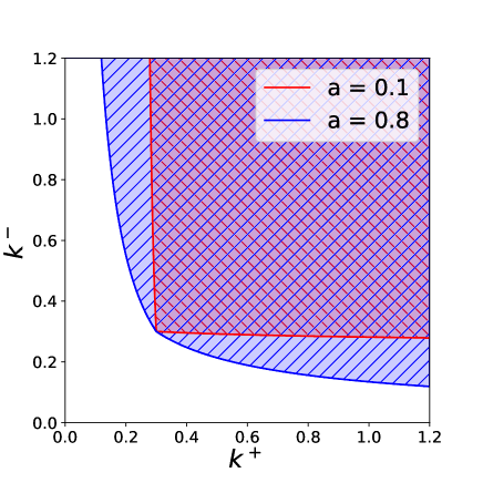
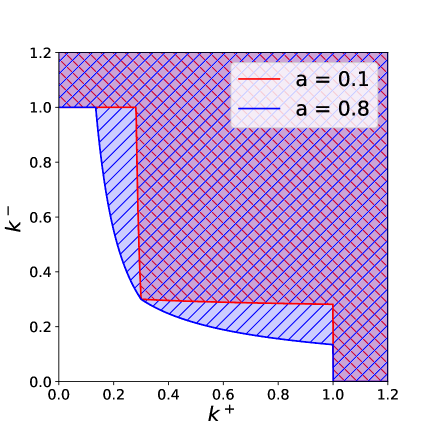
Figure 1: Phase space diagram in the $\{k^{+},k^{-}\}$ plane. The phase space region where there is a virtual contribution but no real radiation is shaded, $a=0.1$ (red) and $a=0.8$ (blue). On the left we show the phase space region without the extra UV regulator, and on the right the region with the extra UV regulator which has been drawn as a hard cutoff $k^{+}\lesssim\nu$, $k^{-}\lesssim\nu$ for illustrative purposes.

The fact that without the extra UV regulator (shown on the left) UV divergences are observable dependent can be understood quite easily from this phase space diagram. The difference between two observables (in the figure represented by the two values $a=0.1$ and $a=0.8$) is computed by integrating over the region shaded blue but not red, which extends all the way to infinity. Thus, the $1/\epsilon$ divergences, and therefore the anomalous dimensions are observable dependent. In the presence of the extra UV regulator (shown on the right) there are no $1/\epsilon$ divergences in the difference between two observables, from which one can expect that the $\mu$ anomalous dimensions are observable independent. The dependence on the extra UV regulator $\nu$, on the other hand, does depend on the observable.

4 Structure of the RGEs and relationship between SCET_I and SCET_II

In this section we will derive and discuss the system of RGE in SCET_I in the presence of the extra UV regulator. We begin by briefly discussing the case of the one loop soft function, where one can explicitly see some of the features introduced to all perturbative orders later.

4.1 An example: the one loop soft function for $a=0$

Consider the soft function Eq. (1) in the case of thrust ($\alpha=\beta=1$) supplemented with the exponential regulator prescription Eq. (50). At one loop in the $\overline{\rm MS}$ scheme,

$$\hat{\cal S}_{\rm bare}(\mu,\nu)=1+2\,\frac{\alpha_{s}(\mu)}{\pi}\,C_{F}\,e^{-\gamma_{E}\frac{Q\tau}{\nu}}\left(\frac{\mu^{2}}{Q\nu}\right)^{\epsilon}\tau^{-1-\epsilon}\frac{\Gamma\left(-\epsilon,\frac{e^{-\gamma_{E}}Q\tau}{\nu}\right)}{\Gamma(1-\epsilon)}\,.$$ (51)

Taking the Laplace transform (6) of the soft function and performing the Laurent expansion for $\epsilon\to 0$ followed by that for $\nu\to\infty$ gives (with $u_{0}=e^{-\gamma_{E}}$)

$$\hat{\cal S}_{\rm bare}(\mu,\nu)=1+\frac{\alpha_{s}(\mu)}{\pi}C_{F}\left(\frac{1}{\epsilon^{2}}+\frac{2}{\epsilon}\,{\ln\frac{\mu}{\nu}}+\ln^{2}\frac{\mu}{\nu}-\ln^{2}\frac{\mu u}{Qu_{0}}+2\ln\frac{\mu}{\nu}\ln\frac{\mu u}{Qu_{0}}-\frac{\pi^{2}}{12}\right)\,.$$ (52)

We now renormalize the $\epsilon$ singularities using the standard procedure outlined in Section 2 and obtain the renormalized soft function

$$\hat{\cal S}_{\rm ren}(\mu,\nu)=1+\frac{\alpha_{s}(\mu)}{\pi}C_{F}\left(\ln^{2}\frac{\mu}{\nu}-\ln^{2}\frac{\mu u}{Qu_{0}}+2\ln\frac{\mu}{\nu}\ln\frac{\mu u}{Qu_{0}}-\frac{\pi^{2}}{12}\right)\,.$$ (53)

It is instructive to first analyze the system of RGEs governing the evolution of the soft function in the $\{\mu,\nu\}$ plane in a fixed coupling approximation, obtaining

$$\frac{{\rm d}\ln\hat{\cal S}_{\rm ren}}{{\rm d}\ln\mu} =4C_{F}\frac{\alpha_{s}(\mu)}{\pi}\ln\frac{\mu}{\nu}\,,$$

$$\frac{{\rm d}\ln\hat{\cal S}_{\rm ren}}{{\rm d}\ln\nu} =-2C_{F}\frac{\alpha_{s}(\mu)}{\pi}\left[\ln\frac{\mu}{\nu}+\ln\frac{\mu u}{Qu_{0}}\right]\,,$$ (54)

where the two differential equations are coupled due to the contribution to the single pole proportional to $\ln\nu$. Using Eq. (2) with $\tau\to u_{0}/u$ in Laplace space, we can write the second of these as

$$\frac{{\rm d}\ln\hat{\cal S}_{\rm ren}}{{\rm d}\ln\nu} =-2C_{F}\frac{\alpha_{s}(\mu)}{\pi}\ln\frac{\mu^{2}}{M_{S}\nu}=-4C_{F}\frac{\alpha_{s}(\mu)}{\pi}\ln\frac{\mu}{\mu(\nu)}\,,$$ (55)

where $\mu(\nu)=M_{S}\sqrt{\nu/N_{S}}=\sqrt{M_{S}\nu}$ (since $N_{S}=M_{S}$) is a new scale that appears in the soft and jet functions, which will be discussed in more detail in the sections below. Including the running coupling effects, the RGEs become

$$\frac{{\rm d}\ln\hat{\cal S}_{\rm ren}}{{\rm d}\ln\mu} =4C_{F}\frac{\alpha_{s}(\mu)}{\pi}\ln\frac{\mu}{\nu}\,,$$

$$\frac{{\rm d}\ln\hat{\cal S}_{\rm ren}}{{\rm d}\ln\nu} =-\int_{\mu(\nu)}^{\mu}\frac{d\mu^{\prime}}{\mu^{\prime}}4C_{F}\frac{\alpha_{s}(\mu^{\prime})}{\pi}\,.$$ (56)

4.2 Evolution equations of SCET_I with a UV regulator for real radiation

As illustrated in the one-loop example of the previous section, in the presence of an additional UV regulator for the real radiation, the soft and jet functions depend both on $\mu$ and $\nu$, and much of the discussion will proceed along very similar lines to what was discussed for the case of SCET_II in Section 2.2, with a few crucial differences. At the canonical scales

$$\mu_{S}=M_{S}\,,\qquad\mu_{J}=M_{J}\,,\qquad\nu_{S}=N_{S}=M_{S}\,,\qquad\nu_{J}=N_{J}=M_{H}\,,$$ (57)

with the $M_{F}$ defined in Eq. (2), the soft and jet functions contain no large logarithms. As in SCET_II, the $\mu$ dependence of the soft and jet functions is obtained by requiring that the bare functions are independent of the scale $\mu$, leading to Eq. (27), repeated here for convenience

$$\frac{{\rm d}}{{\rm d}\ln\mu}\ln F_{{\rm sub}}(\mu,\nu)=-\frac{{\rm d}}{{\rm d}\ln\mu}\ln Z_{F}(\mu,\nu)=\gamma^{(\mu)}_{F}(\mu,\nu)\,,$$ (58)

with $F=\hat{\cal S},\,\hat{\cal J}_{n},\,\hat{\cal J}_{\bar{n}}$. The form of the anomalous dimensions $\gamma^{(\mu)}_{F}(\mu,\nu)$ are also the same as in SCET_II,

$$\gamma^{(\mu)}_{S}(\mu,\nu) =4\Gamma_{\rm cusp}[\alpha_{s}(\mu)]\ln\frac{\mu}{\nu}+\widehat{\gamma}_{S}[\alpha_{s}(\mu)]\,,$$

$$\gamma^{(\mu)}_{J}(\mu,\nu) =2\Gamma_{\rm cusp}[\alpha_{s}(\mu)]\ln\frac{\nu}{N_{J}}+\widehat{\gamma}_{J}[\alpha_{s}(\mu)]\,.$$ (59)

However, extra care must be taken because, contrary to SCET_II, one has

$$\mu_{S}\sim M_{S}\neq M_{J}\sim\mu_{J}\,.$$ (60)

In particular, the arguments given at the end of Section 2.2 leading to the general form for the soft and jet functions need to be revisited. Following similar arguments as in SCET_II one can show that the most general form has to be

$$\ln\hat{\cal S}(\mu,\nu) =\ln\widetilde{\cal S}(\mu/M_{S})+\int_{N_{S}}^{\nu}\frac{{\rm d}\nu^{\prime}}{\nu^{\prime}}\,c(\mu/\mu_{S}(\nu))\,,$$

$$\ln\hat{\cal J}(\mu,\nu) =\ln\widetilde{\cal J}(\mu/M_{J})-\frac{1}{2}\int_{N_{J}}^{\nu}\frac{{\rm d}\nu^{\prime}}{\nu^{\prime}}\,c(\mu/\mu_{J}(\nu))\,.$$ (61)

and we introduced the new scales $\mu_{S}(\nu)$ and $\mu_{J}(\nu)$ such that $\mu_{S}(\nu)=\mu_{J}(\nu)\equiv\mu(\nu)$, in order for the $\nu$ dependence to cancel in the combination of the soft and jet functions. Each function in the above equation also depends on $\alpha_{s}(\mu)$ which can in turn be re-expressed in terms of $\alpha_{s}(\mu(\nu))$ in all quantities (upon changing the functional dependence on $\mu/\mu(\nu)$). Since the dependence on $\mu$ and $\nu$ is always through the ratio with $M_{F}$ and $N_{F}$, by dimensional analysis the most general form for $\mu_{F}(\nu)$ is

$$\mu_{F}(\nu)=M_{F}\,f(\nu/N_{F})\,,$$ (62)

and one needs to find a function $f$ for which $\mu_{S}(\nu)=\mu_{J}(\nu)$.

In order for the function $F(M_{F},N_{F})$ to be free of large logarithms one requires $\mu_{F}(N_{F})=M_{F}$ and therefore $f(1)=1$. The functional form for the function $f$ can be found by evaluating $\mu_{F}(\nu)$ for $\nu=N_{J}=M_{H}$. This gives

$$\mu_{S}(\nu=M_{H})=M_{S}\,f(M_{H}/M_{S})\overset{!}{=}\mu_{J}(\nu=M_{H})=M_{J}f(M_{H}/M_{H})=M_{J}\,.$$ (63)

Using Eq. (2), this immediately implies $f(z)=z^{\beta/(\alpha+\beta)}$, therefore

$$\mu_{F}(\nu)=M_{F}\left(\frac{\nu}{N_{F}}\right)^{\frac{\beta}{\alpha+\beta}}\,,$$ (64)

and $\mu_{F}(\nu)$ is in fact independent of $F$

$$\mu(\nu)\equiv\mu_{S}(\nu)=\mu_{J}(\nu)=\nu^{\frac{\beta}{\alpha+\beta}}Q^{\frac{\alpha}{\alpha+\beta}}\tau^{\frac{1}{\alpha+\beta}}\,.$$ (65)

From this discussion one sees that the results are very similar to the SCET_II case, with the only difference being that the derivatives with respect to $\nu$ are functions of $\mu/\mu_{F}(\nu)$, rather than $\mu/M_{F}$.

Given this, one can now write the solution to the differential equation Eq. (58) as

$$F_{{\rm sub}}(\mu,\nu) =F_{{\rm sub}}(\mu_{F}(\nu),\nu)\exp\left[\int_{\mu_{F}(\nu)}^{\mu}\frac{{\rm d}\mu^{\prime}}{\mu^{\prime}}\gamma^{(\mu)}_{F}(\mu^{\prime},\nu)\right]$$

$$\equiv F_{{\rm sub}}(\mu_{F}(\nu),\nu)U_{F}(\mu_{F}(\nu),\mu;\nu)\,,$$ (66)

but as in SCET_II it is not sufficient to perform the resummation. A second differential equation in the new regularization scale $\nu$ can however be derived as in Sec. 2.2 by taking the $\nu$ derivative of the resummed result $F_{{\rm sub}}(\mu,\nu)$

$$\frac{{\rm d}}{{\rm d}\ln\nu}F_{{\rm sub}}(\mu,\nu) =\left[\frac{\partial\ln\mu_{F}(\nu)}{\partial\ln\nu}\gamma_{F}^{(\mu)}(\mu_{F}(\nu),\nu)F_{{\rm sub}}(\mu,\nu)+U_{F}(\mu_{F}(\nu),\mu;\nu)\frac{\partial}{\partial\ln\nu}F_{{\rm sub}}(\mu_{F}(\nu),\nu)\right]$$

$$\qquad+\left[-\frac{\partial\ln\mu_{F}(\nu)}{\partial\ln\nu}\gamma_{F}^{(\mu)}(\mu_{F}(\nu),\nu)+\int_{\mu_{F}(\nu)}^{\mu}\frac{{\rm d}\mu^{\prime}}{\mu^{\prime}}\frac{\partial}{\partial\ln\nu}\,\gamma^{(\mu)}_{F}(\mu^{\prime},\nu)\right]F_{{\rm sub}}(\mu,\nu)$$

$$=F_{{\rm sub}}(\mu,\nu)\left[\frac{\partial}{\partial\ln\nu}\ln F_{{\rm sub}}(\mu_{F}(\nu),\nu)+\int_{\mu_{F}(\nu)}^{\mu}\frac{{\rm d}\mu^{\prime}}{\mu^{\prime}}\frac{\partial}{\partial\ln\nu}\,\gamma^{(\mu)}_{F}(\mu^{\prime},\nu)\right]\,.$$ (67)

One can define in analogy with Eq. (36)

$$\frac{\partial}{\partial\ln\nu}\ln F_{{\rm sub}}(\mu_{F}(\nu),\nu)\equiv a_{F}\,\gamma^{(\nu)}_{\alpha,\beta}[\alpha_{s}(\mu_{F}(\nu))]\,,$$ (68)

with $a_{F}$ given in Eq. (34). This is possible because $\mu_{F}(\nu)$ is the same function for the soft and jet sector, and because the $\nu$ dependence cancels between the two sectors. We therefore obtain from Eq. (67)

$$\frac{{\rm d}}{{\rm d}\ln\nu}\ln F_{{\rm sub}}(\mu,\nu) =a_{F}\,\left[\gamma^{(\nu)}_{\alpha,\beta}[\alpha_{s}(\mu_{F}(\nu))]-2\int_{\mu_{F}(\nu)}^{\mu}\frac{{\rm d}\mu^{\prime}}{\mu^{\prime}}\,\Gamma_{\rm cusp}[\alpha_{s}(\mu^{\prime})]\right]$$

$$\equiv\gamma^{(\nu)}_{\alpha,\beta;F}(\mu,\nu)\,,$$ (69)

analogous to Eq. (37).

With the dependence of $F_{{\rm sub}}(\mu(\nu),\nu)$ on $\mu$ and $\nu$, given in Eqs. (58) and (4.2), respectively, one can sum all logarithms by performing the integration along the path $(\mu_{F},\nu_{F})\to(\mu,\nu_{F})\to(\mu,\nu)$, just as was done for SCET_II. This gives

$$U_{F}(\mu_{F},\nu_{F};\mu,\nu)=U_{F}^{(\mu)}(\mu_{F},\mu;\nu_{F})U_{F}^{(\nu)}(\nu_{F},\nu;\mu)\,,$$ (70)

with

$$\ln U_{S}^{(\mu)}(\mu_{S},\mu;\nu_{S}) =\int_{\mu_{S}}^{\mu}\frac{{\rm d}\mu^{\prime}}{\mu^{\prime}}\left[4\Gamma_{\rm cusp}[\alpha_{s}(\mu^{\prime})]\ln\frac{\mu^{\prime}}{\nu_{S}}+\widehat{\gamma}_{S}[\alpha_{s}(\mu^{\prime})]\right]\,,$$ (71a)

$$\ln U_{J}^{(\mu)}(\mu_{J},\mu;\nu_{J}) =\int_{\mu_{J}}^{\mu}\frac{{\rm d}\mu^{\prime}}{\mu^{\prime}}\widehat{\gamma}_{J}[\alpha_{s}(\mu)]\,,$$ (71b)

$$\ln U_{S}^{(\nu)}(\nu_{S},\nu;\mu) =\int_{\nu_{S}}^{\nu}\frac{{\rm d}\nu^{\prime}}{\nu^{\prime}}\left[-4\int_{\mu(\nu^{\prime})}^{\mu}\frac{{\rm d}\mu^{\prime}}{\mu^{\prime}}\Gamma_{\rm cusp}[\alpha_{s}(\mu^{\prime})]+2\gamma^{(\nu)}_{\alpha,\beta}[\alpha_{s}(\mu(\nu^{\prime}))]\right]\,,$$ (71c)

$$\ln U_{J}^{(\nu)}(\nu_{J},\nu;\mu) =\int_{\nu_{J}}^{\nu}\frac{{\rm d}\nu^{\prime}}{\nu^{\prime}}\left[2\int_{\mu(\nu^{\prime})}^{\mu}\frac{{\rm d}\mu^{\prime}}{\mu^{\prime}}\Gamma_{\rm cusp}[\alpha_{s}(\mu^{\prime})-\gamma^{(\nu)}_{\alpha,\beta}[\alpha_{s}(\mu(\nu^{\prime}))]\right]\,.$$ (71d)

$U_{J}^{(\mu)}(\mu_{J},\mu;\nu_{J})$ has no term proportional to the cusp anomalous dimension. The factorization theorem Eq. (5) in the presence of the extra UV regulator takes the same form as SCET_II Eq. (43), namely

$$\hat{\sigma}[u]=H(\mu_{H})U_{H}^{2}(\mu_{H},\mu)\,\hat{\cal J}_{n}(\mu_{J},\nu_{J})\hat{\cal J}_{\bar{n}}(\mu_{J},\nu_{J})\,U_{J}(\mu_{S},\nu_{S},\mu,\nu)\,\hat{\cal S}(\mu_{S},\nu_{S})\,U_{S}(\mu_{S},\nu_{S},\mu,\nu)\,,$$ (72)

and as before we have not explicitly shown the dependence on the scales $M_{H},M_{J},M_{S}$.

It is illustrative to compare these equations with the SCET_II equations obtained in Sec. 2.2. The crucial difference is that the scales $\mu_{F}$ that appeared in the functions $U_{F}^{(\nu)}$ are now replaced by the scale $\mu(\nu)$ that is common to the soft and zero-bin subtracted jet functions. As already mentioned, this is a consequence of the fact that the dependence on the new unphysical regularization scale $\nu$ must cancel in their combination. In the following section we will discuss the implications of introducing an extra UV regulator in the effective theory.

5 Implications of the $\nu$ regulator on SCET_I

We have shown that with the introduction of a suitably defined UV regulator into SCET_I theories, resummation of large logarithms can be achieved via a system of RGEs that involves two types of anomalous dimensions, namely the $\mu$ anomalous dimensions

$$\gamma^{(\mu)}_{S}(\mu,\nu) =4\Gamma_{\rm cusp}[\alpha_{s}(\mu)]\ln\frac{\mu}{\nu}+\widehat{\gamma}_{S}[\alpha_{s}(\mu)]\,,$$

$$\gamma^{(\mu)}_{J}(\mu,\nu) =2\Gamma_{\rm cusp}[\alpha_{s}(\mu)]\ln\frac{\nu}{N_{J}}+\widehat{\gamma}_{J}[\alpha_{s}(\mu)]\,,$$ (73)

and the $\nu$ anomalous dimension

$$\gamma^{(\nu)}_{\alpha,\beta;F}(\mu,\nu)=a_{F}\,\left[\gamma^{(\nu)}_{\alpha,\beta}[\alpha_{s}(\mu(\nu))]-2\int_{\mu(\nu)}^{\mu}\frac{{\rm d}\mu^{\prime}}{\mu^{\prime}}\,\Gamma_{\rm cusp}[\alpha_{s}(\mu^{\prime})]\right]\,.$$ (74)

This has a number of implications that we would like to comment upon below and in more detail in the subsections that follow.

Observable (in)dependence of the anomalous dimensions, and implications for multi-leg processes.

As was already discussed, the extra regulator handles all UV divergences in the real contributions to operator matrix elements, while not affecting the virtual corrections. This implies that the $\mu$ anomalous dimension is related to the virtual diagrams, and therefore independent of the observable, which only affects real phase space integrals. It is therefore identical to the $\mu$ anomalous dimension in SCET_II problems, that does not depend on the specific constraint on the real radiation. The term in $\gamma^{(\nu)}_{\alpha,\beta;F}$ proportional to the cusp anomalous dimension is also universal, and only depends on the observable through the definition of the scale $\mu(\nu)$ given in Eq. (64). All observable dependence is therefore contained in the non-cusp term of the $\nu$ anomalous dimension Eq. (74), which is determined by the real contributions to the matrix elements of operators. As discussed, this $\nu$ dependence has to cancel between the jet and soft functions, and as we will see shortly it can be seen to arise from the zero-bin region Manohar:2006nz of phase space integrals, which are expanded simultaneously around the soft and collinear limit, and are therefore significantly easier to compute. This observation is particularly useful when tackling the computation for multi-leg processes, in which case the factorization theorem will be of the (schematic) form

$$\sigma\sim\mathbf{H}\,{\cal\mathbf{S}}\,\prod_{i}{\cal J}_{n_{i}}\,,$$ (75)

where now the hard and soft functions will be matrices in color space. In this case, the considerations above suggest that the observable dependence of the anomalous dimensions is entirely of soft-collinear origin and it can be extracted from a calculation of the zero-bin subtraction Manohar:2006nz in the presence of the extra UV regulator, which is a diagonal quantity in color space, and hence would not require the explicit computation of the more complicated soft function. We leave the exploration of this property to future work.

Connection to SCET_I.

While one can directly perform the resummation in SCET_I in the presence of the extra UV regulator, one can also connect the new system of RGEs to the standard SCET_I case regularized in dimensional regularization. This results in an interesting connection between the anomalous dimensions obtained with and without the extra UV regulator. As will be shown in detail in Section 5.1, and explicitly at 2-loop order in Section 6, this can be used to carry out the direct derivation of SCET_I anomalous dimensions starting from a computation in the presence of the extra UV regulator. This property can become quite useful for perturbative calculations.

Numerical resummation.

Another important feature discussed in more detail in the next section is that when we perform the explicit 2-loop calculation of the soft function, the observable dependence can be computed by dividing the real phase space integrals into different separate contributions. One can for instance define a first contribution where a simplified version of the observable is used rather than the full observable. This simplified observable only depends on the singular scaling of the original observable and is therefore universal and gives rise to much simpler integrals. The observable dependence in this contribution can be determined relatively straightforwardly. The second contribution, that we call non-inclusive, computes the difference of the full observable to the simplified version. While this contribution depends on the full details of the observable, the difference is infrared and collinear finite, hence allowing one to perform the computation numerically in a rather efficient fashion. This observation is the basis of the numerical resummation technique developed recently in the framework of SCET Bauer:2018svx ; Bauer:2019bsp .

5.1 Zero-bin subtraction and refactorization: relation with standard SCET_I

We now relate the system of RGEs given by Eqs. (58), (4.2) to the standard SCET_I case in pure dimensional regularization. The solutions to the equations in Eqs. (71) sum the logarithmic corrections in a form that is similar for both SCET_I and SCET_II. To compare with the usual SCET_I form, we invert the order of the $\nu$ and $\mu$ integration in the $\nu$ evolution equations Eq. (71c) and Eq. (71d). From now on we will always assume $\mu_{S}=M_{S}$, $\mu_{J}=M_{J}$ and $\mu_{H}=M_{H}$, as well as $\nu_{J}=M_{H}$ and $\nu_{S}=M_{S}$, and use the notation interchangeably. Using Eq. (64) one can write

$$\int_{\nu_{F}}^{\nu}\frac{{\rm d}\nu^{\prime}}{\nu^{\prime}}\int_{\mu(\nu^{\prime})}^{\mu}\frac{{\rm d}\mu^{\prime}}{\mu^{\prime}}=\left\{\begin{array}[]{ll}\int_{\mu_{F}}^{\mu}\frac{{\rm d}\mu^{\prime}}{\mu^{\prime}}\int_{\nu_{F}}^{\nu(\mu^{\prime})}\frac{{\rm d}\nu^{\prime}}{\nu^{\prime}}+\int_{\mu(\nu)}^{\mu}\frac{{\rm d}\mu^{\prime}}{\mu^{\prime}}\int_{\nu(\mu^{\prime})}^{\nu}\frac{{\rm d}\nu^{\prime}}{\nu^{\prime}}&\beta\neq 0\\ \int_{\mu_{F}}^{\mu}\frac{{\rm d}\mu^{\prime}}{\mu^{\prime}}\int_{\nu_{F}}^{\nu}\frac{{\rm d}\nu^{\prime}}{\nu^{\prime}}&\beta=0\end{array}\right.\,,$$ (78)

with $\nu(\mu)$ being the inverse of $\mu(\nu)$

$$\nu(\mu)=\nu_{F}\left(\frac{\mu}{\mu_{F}}\right)^{\frac{\alpha+\beta}{\beta}}\,.$$ (79)

Note that we had to distinguish between $\beta=0$ (SCET_II) and $\beta\neq 0$ (SCET_I), since for $\beta=0$ the quantity $\nu(\mu)$ is clearly not defined and $\mu(\nu)$ is independent of $\nu$.

For $\beta\neq 0$ we can rewrite the solution to the $\nu$ evolution as

$$\ln U_{S}^{(\nu)}(\nu_{S},\nu;\mu) =-4\frac{\alpha+\beta}{\beta}\int_{\mu_{S}}^{\mu}\frac{{\rm d}\mu^{\prime}}{\mu^{\prime}}\Gamma_{\rm cusp}[\alpha_{s}(\mu^{\prime})]\ln\frac{\mu^{\prime}}{\mu_{S}}$$ (80)

$$\qquad+4\frac{\alpha+\beta}{\beta}\int_{\mu(\nu)}^{\mu}\frac{{\rm d}\mu^{\prime}}{\mu^{\prime}}\Gamma_{\rm cusp}[\alpha_{s}(\mu^{\prime})]\ln\frac{\mu^{\prime}}{\mu(\nu)}+2\int_{\nu_{S}}^{\nu}\frac{{\rm d}\nu^{\prime}}{\nu^{\prime}}\gamma^{(\nu)}_{\alpha,\beta}[\alpha_{s}(\mu(\nu^{\prime}))]\,,$$

$$\ln U_{J}^{(\nu)}(\nu_{S},\nu;\mu) =2\frac{\alpha+\beta}{\beta}\int_{\mu_{J}}^{\mu}\frac{{\rm d}\mu^{\prime}}{\mu^{\prime}}\Gamma_{\rm cusp}[\alpha_{s}(\mu^{\prime})]\ln\frac{\mu^{\prime}}{\mu_{J}}$$

$$\qquad-2\frac{\alpha+\beta}{\beta}\int_{\mu(\nu)}^{\mu}\frac{{\rm d}\mu^{\prime}}{\mu^{\prime}}\Gamma_{\rm cusp}[\alpha_{s}(\mu^{\prime})]\ln\frac{\mu^{\prime}}{\mu(\nu)}-\int_{\nu_{J}}^{\nu}\frac{{\rm d}\nu^{\prime}}{\nu^{\prime}}\gamma^{(\nu)}_{\alpha,\beta}[\alpha_{s}(\mu(\nu^{\prime}))]\,,$$

where we have used

$$\ln\frac{\nu(\mu)}{\nu_{F}}=\frac{\alpha+\beta}{\beta}\ln\frac{\mu}{\mu_{F}}\,,\qquad\ln\frac{\nu}{\nu(\mu)}=-\frac{\alpha+\beta}{\beta}\ln\frac{\mu}{\mu(\nu)}\,,$$ (81)

which follow directly from Eqs. (64) and (79). Using this in Eq. (70) one finds

$$\ln U_{S}(\mu_{S},\nu_{S};\mu,\nu) =\int_{\mu_{S}}^{\mu}\frac{{\rm d}\mu^{\prime}}{\mu^{\prime}}\left[-4\,\frac{\alpha}{\beta}\,\Gamma_{\rm cusp}[\alpha_{s}(\mu^{\prime})]\ln\frac{\mu^{\prime}}{\mu_{S}}+\widehat{\gamma}_{S}[\alpha_{s}(\mu^{\prime})]\right]$$ (82)

$$\quad+4\frac{\alpha+\beta}{\beta}\int_{\mu(\nu)}^{\mu}\frac{{\rm d}\mu^{\prime}}{\mu^{\prime}}\,\Gamma_{\rm cusp}[\alpha_{s}(\mu^{\prime})]\ln\frac{\mu^{\prime}}{\mu(\nu)}+2\int_{\nu_{S}}^{\nu}\frac{{\rm d}\nu^{\prime}}{\nu^{\prime}}\gamma^{(\nu)}_{\alpha,\beta}[\alpha_{s}(\mu(\nu^{\prime}))]\,,$$

$$\ln U_{J}(\mu_{J},\nu_{J};\mu,\nu) =\int_{\mu_{J}}^{\mu}\frac{{\rm d}\mu^{\prime}}{\mu^{\prime}}\left[2\,\frac{\alpha+\beta}{\beta}\,\Gamma_{\rm cusp}[\alpha_{s}(\mu^{\prime})]\ln\frac{\mu^{\prime}}{\mu_{J}}+\widehat{\gamma}_{J}[\alpha_{s}(\mu^{\prime})]\right]$$

$$\quad-2\frac{\alpha+\beta}{\beta}\int_{\mu(\nu)}^{\mu}\frac{{\rm d}\mu^{\prime}}{\mu^{\prime}}\Gamma_{\rm cusp}[\alpha_{s}(\mu^{\prime})]\ln\frac{\mu^{\prime}}{\mu(\nu)}-\int_{\nu_{J}}^{\nu}\frac{{\rm d}\nu^{\prime}}{\nu^{\prime}}\gamma^{(\nu)}_{\alpha,\beta}[\alpha_{s}(\mu(\nu^{\prime}))]\,.$$

The first line in each of the two parts of Eq. (82) starts resembling the usual SCET_I evolution with an integration over ${\rm d}\ln\!\mu$ between the scales $\mu_{F}$ and $\mu$, and an anomalous dimension that depends on $\alpha$ and $\beta$. The second line in each equation on the other hand does not have this form. Using Eq. (64), however, one can change the integration variable from $\nu$ to $\mu(\nu)$

$$\int_{\nu_{F}}^{\nu}\frac{{\rm d}\nu}{\nu}f(\nu) =\frac{\alpha+\beta}{\beta}\int_{\mu_{F}}^{\mu(\nu)}\frac{{\rm d}\mu(\nu)}{\mu(\nu)}f(\nu(\mu))\,.$$ (83)

This leads to

$$\ln U_{S}(\mu_{S},\nu_{S};\mu,\nu) =\int_{\mu_{S}}^{\mu}\frac{{\rm d}\mu^{\prime}}{\mu^{\prime}}\left[-4\,\frac{\alpha}{\beta}\,\Gamma_{\rm cusp}[\alpha_{s}(\mu^{\prime})]\ln\frac{\mu^{\prime}}{\mu_{S}}+\widetilde{\gamma}_{\alpha,\beta;S}[\alpha_{s}(\mu^{\prime})]\right]+2R_{\alpha,\beta}(\mu(\nu);\mu)\,,$$

$$\ln U_{J}(\mu_{J},\nu_{J},\mu,\nu) =\int_{\mu_{J}}^{\mu}\frac{{\rm d}\mu^{\prime}}{\mu^{\prime}}\left[2\,\frac{\alpha+\beta}{\beta}\,\Gamma_{\rm cusp}[\alpha_{s}(\mu^{\prime})]\ln\frac{\mu^{\prime}}{\mu_{J}}+\widetilde{\gamma}_{\alpha,\beta;J}[\alpha_{s}(\mu^{\prime})]\right]-R_{\alpha,\beta}(\mu(\nu);\mu)\,,$$ (84)

where we have used (79) and defined

$$\widetilde{\gamma}_{\alpha,\beta;S}[\alpha_{s}(\mu)] =\widehat{\gamma}_{S}[\alpha_{s}(\mu)]+2\,\frac{\alpha+\beta}{\beta}\,\gamma^{(\nu)}_{\alpha,\beta}[\alpha_{s}(\mu)]\,,$$

$$\widetilde{\gamma}_{\alpha,\beta;J}[\alpha_{s}(\mu)] =\widehat{\gamma}_{J}[\alpha_{s}(\mu)]-\frac{\alpha+\beta}{\beta}\,\gamma^{(\nu)}_{\alpha,\beta}[\alpha_{s}(\mu)]\,,$$ (85)

and

$$R_{\alpha,\beta}(\mu(\nu);\mu)=\frac{\alpha+\beta}{\beta}\int_{\mu(\nu)}^{\mu}\frac{{\rm d}\mu^{\prime}}{\mu^{\prime}}\left[2\,\Gamma_{\rm cusp}[\alpha_{s}(\mu^{\prime})]\ln\frac{\mu^{\prime}}{\mu(\nu)}-\gamma^{(\nu)}_{\alpha,\beta}[\alpha_{s}(\mu^{\prime})]\right]\,.$$ (86)

Eq. (5.1) indicates that the evolution operator of each of the soft and jet functions in the SCET_I case ($\beta\neq 0$) can be factorized into the product in Laplace space of a term that only depends on the ratio of scales $\mu/\mu_{F}$ and a term $R(\mu(\nu);\mu)$ that depends on the ratio $\mu/\mu(\nu)$ which cancels in the physical cross section.

In order to complete this re-factorization, we need to consider the factorization of the initial condition to the soft and jet functions in (72) which, as already explained, depends on two canonical scales $\mu_{F}$, $\nu_{F}$. The full soft and jet function in the presence of the extra UV regulator can be written in terms of those in standard SCET_I as

$$\hat{\cal S}(\mu_{S},\nu_{S};\mu,\nu) =\hat{\cal S}_{\rm SCET_{I}}(\mu_{S};\mu)\Delta_{\alpha,\beta;S}(\mu_{S},\nu_{S};\mu,\nu)\,,$$

$$\hat{\cal J}(\mu_{J},\nu_{J};\mu,\nu) =\hat{\cal J}_{\rm SCET_{I}}(\mu_{J};\mu)\Delta_{\alpha,\beta;J}(\mu_{J},\nu_{J};\mu,\nu)\,,$$ (87)

which defines the functions $\Delta_{\alpha,\beta;F}(\mu_{F},\nu_{F};\mu,\nu)$. Given the importance of the scale dependence in the soft and functions in what follows, we show them explicitly in these equations. Using, as before, the fact that the $\nu$ dependence cancels in the combination of jet and soft functions, leads to the important relations 

$$\Delta_{\alpha,\beta;S}(\mu_{S},\nu_{S};\mu,\nu)=\Delta_{\alpha,\beta}^{2}(\mu(\nu);\mu)\,,\qquad\Delta_{\alpha,\beta;J}(\mu_{J},\nu_{J};\mu,\nu)=\Delta_{\alpha,\beta}^{-1}(\mu(\nu);\mu)\,,$$ (88)

and that the function $\Delta_{\alpha,\beta}$ has no large logarithms when evaluated at the scale $\mu=\mu(\nu)$. Given this general form, one can write the evolution kernel for the soft sector as (and similarly for the collinear sector)

$$U_{S}(\mu_{S},\nu_{S},\mu,\nu) =\frac{\hat{\cal S}(\mu_{S},\nu_{S};\mu,\nu)}{\hat{\cal S}(\mu_{S},\nu_{S};\mu_{S},\nu_{S})}$$ (89)

$$=\frac{\hat{\cal S}_{\rm SCET_{I}}(\mu_{S};\mu)}{\hat{\cal S}_{\rm SCET_{I}}(\mu_{S};\mu_{S})}\frac{\Delta_{\alpha,\beta}^{2}(\mu(\nu);\mu)}{\Delta_{\alpha,\beta}^{2}(\mu(\nu_{S});\mu_{S})}$$

$$=U^{\rm SCET_{I}}_{S}(\mu_{S},\mu)\frac{\Delta_{\alpha,\beta}^{2}(\mu(\nu);\mu)}{\Delta_{\alpha,\beta}^{2}(\mu(\nu);\mu(\nu))}\frac{\Delta_{\alpha,\beta}^{2}(\mu(\nu);\mu(\nu))}{\Delta_{\alpha,\beta}^{2}(\mu;\mu)}\frac{\Delta_{\alpha,\beta}^{2}(\mu;\mu)}{\Delta_{\alpha,\beta}^{2}(\mu_{S};\mu_{S})}$$

$$=\left[U^{\rm SCET_{I}}_{S}(\mu_{S},\mu)\frac{\Delta_{\alpha,\beta}^{2}(\mu;\mu)}{\Delta_{\alpha,\beta}^{2}(\mu_{S};\mu_{S})}\right]\left[\frac{\Delta_{\alpha,\beta}^{2}(\mu(\nu);\mu)}{\Delta_{\alpha,\beta}^{2}(\mu(\nu);\mu(\nu))}\frac{\Delta_{\alpha,\beta}^{2}(\mu(\nu);\mu(\nu))}{\Delta_{\alpha,\beta}^{2}(\mu;\mu)}\right]\,,$$

where we have used that $\mu(\nu_{F})=\mu_{F}$. Here the term in the first square bracket only depends on the scales $\mu$ and $\mu_{S}$, while the one in the second square bracket depends on the scales $\mu$ and $\mu(\nu)$. Since $\Delta(\mu(\nu);\mu(\nu))$ has no large logarithms, we can write it as

$$\Delta_{\alpha,\beta}[\alpha_{s}(\mu(\nu))]\equiv\Delta_{\alpha,\beta}(\mu(\nu);\mu(\nu))=1+\sum_{n=1}\left(\frac{\alpha_{s}(\mu(\nu))}{4\pi}\right)^{n}d_{\alpha,\beta}^{(n)}\,,$$ (90)

where the coefficients $d_{\alpha,\beta}^{(n)}$ can be obtained by taking the ratio between the SCET_I initial conditions with and without the $\nu$ regulator. This means that we can write

$$\frac{\Delta_{\alpha,\beta}(\mu_{1};\mu_{1})}{\Delta_{\alpha,\beta}(\mu_{2};\mu_{2})}=\exp\left\{\int_{\mu_{2}}^{\mu_{1}}\frac{{\rm d}\mu^{\prime}}{\mu^{\prime}}2\beta[\alpha_{s}(\mu^{\prime})]\frac{{\rm d}\ln\Delta_{\alpha,\beta}}{{\rm d}\alpha_{s}}\right\}\,,$$ (91)

where ${{\rm d}\ln\Delta_{\alpha,\beta}}/{{\rm d}\alpha_{s}}$ is a function of $\alpha_{s}$. The QCD $\beta$ function is given by

$$\beta[\alpha_{s}(\mu)]=\frac{{\rm d}\alpha_{s}(\mu)}{{\rm d}\ln\mu^{2}}=-\alpha_{s}(\mu)\left(b_{0}\frac{\alpha_{s}(\mu)}{4\pi}+\dots\right)\,,$$ (92)

where $b_{0}=(11C_{A}-2n_{F})/3$. This allows us to write

$$\ln U_{S}(\mu_{S},\nu_{S},\mu,\nu) =\left[\ln U^{\rm SCET_{I}}_{S}(\mu_{S},\mu)+2\int_{\mu_{S}}^{\mu}\frac{{\rm d}\mu^{\prime}}{\mu^{\prime}}2\beta[\alpha_{s}(\mu^{\prime})]\frac{{\rm d}\ln\Delta_{\alpha,\beta}}{{\rm d}\alpha_{s}}\right]$$ (93)

$$\qquad+\left[2\ln\frac{\Delta_{\alpha,\beta}(\mu(\nu);\mu)}{\Delta_{\alpha,\beta}(\mu(\nu);\mu(\nu))}-2\int_{\mu(\nu)}^{\mu}\frac{{\rm d}\mu^{\prime}}{\mu^{\prime}}2\beta[\alpha_{s}(\mu^{\prime})]\frac{{\rm d}\ln\Delta_{\alpha,\beta}}{{\rm d}\alpha_{s}}\right]\,.$$

Comparing this result to Eq. (5.1), and equating the terms that involve the evolution between $\mu_{S}$ and $\mu$ and the ones that involve the $\mu(\nu)\to\mu$ evolution, one can read off

$$\ln U_{S}^{\rm SCET_{I}}(\mu_{S};\mu) =\int_{\mu_{S}}^{\mu}\frac{{\rm d}\mu^{\prime}}{\mu^{\prime}}\left[-4\,\frac{\alpha}{\beta}\,\Gamma_{\rm cusp}[\alpha_{s}(\mu^{\prime})]\ln\frac{\mu^{\prime}}{\mu_{S}}+\widetilde{\gamma}_{\alpha,\beta;S}[\alpha_{s}(\mu^{\prime})]-4\beta[\alpha_{s}(\mu^{\prime})]\frac{{\rm d}\ln\Delta_{\alpha,\beta}}{{\rm d}\alpha_{s}}\right]\,,$$

$$\ln\frac{\Delta_{\alpha,\beta}(\mu(\nu);\mu)}{\Delta_{\alpha,\beta}(\mu(\nu);\mu(\nu))} =R_{\alpha,\beta}(\mu(\nu);\mu)+\int_{\mu(\nu)}^{\mu}\frac{{\rm d}\mu^{\prime}}{\mu^{\prime}}2\beta[\alpha_{s}(\mu^{\prime})]\frac{{\rm d}\ln\Delta_{\alpha,\beta}}{{\rm d}\alpha_{s}}\,.$$ (94)

From this, we obtain the anomalous dimension in standard SCET_I (see Eq. (2.1)), and the non-cusp pieces $\widehat{\gamma}_{\alpha,\beta;F}^{\rm SCET_{I}}$ are

$$\widehat{\gamma}_{\alpha,\beta;S}^{\rm SCET_{I}}[\alpha_{s}(\mu)] =\widetilde{\gamma}_{\alpha,\beta;S}[\alpha_{s}(\mu)]-4\beta[\alpha_{s}(\mu)]\frac{{\rm d}\ln\Delta_{\alpha,\beta}}{{\rm d}\alpha_{s}}$$

$$=\widehat{\gamma}_{S}[\alpha_{s}(\mu)]+2\,\frac{\alpha+\beta}{\beta}\,\gamma^{(\nu)}_{\alpha,\beta}[\alpha_{s}(\mu)]-4\beta[\alpha_{s}(\mu)]\frac{{\rm d}\ln\Delta_{\alpha,\beta}}{{\rm d}\alpha_{s}}\,,$$

$$\widehat{\gamma}_{\alpha,\beta;J}^{\rm SCET_{I}}[\alpha_{s}(\mu)] =\widetilde{\gamma}_{\alpha,\beta;J}[\alpha_{s}(\mu)]+2\beta[\alpha_{s}(\mu)]\frac{{\rm d}\ln\Delta_{\alpha,\beta}}{{\rm d}\alpha_{s}}$$

$$=\widehat{\gamma}_{J}[\alpha_{s}(\mu)]-\,\frac{\alpha+\beta}{\beta}\,\gamma^{(\nu)}_{\alpha,\beta}[\alpha_{s}(\mu)]+2\beta[\alpha_{s}(\mu)]\frac{{\rm d}\ln\Delta_{\alpha,\beta}}{{\rm d}\alpha_{s}}\,,$$ (95)

where we have used Eq. (5.1) and analogous arguments to obtain the jet anomalous dimension.

Eqs. (5.1) relate the anomalous dimensions calculated with the additional $\nu$ regulator to the standard SCET_I result calculated in dimensional regularization. Notice that due to the presence of $\beta[\alpha_{s}(\mu)]$ in the last term, to compute an anomalous dimension at $k$-th order one only requires the initial condition for $\Delta_{\alpha,\beta}$ at $(k-1)$-th order. It is important to stress again that the above discussion relating the system of RGEs in the presence of a UV regulator to the standard RGE is clearly not allowed when $\beta=0$ (i.e. in SCET_II), in which case one is forced to keep a coupled system of evolution equations.

The above discussion highlights an important point: as mentioned in Section 2.1, SCET_I is characterized by a scale separation between the soft and the collinear sectors. In particular, if $M_{J}\gg M_{S}$ the two jet functions can be interpreted as a matching coefficient between SCET_I and the lower-energy purely soft theory, described by the soft function. The introduction of the extra UV regulator, however, introduces a new scale $\mu(\nu)$ that interpolates between the soft scale $M_{S}$ and the collinear scale $M_{J}$ depending on the value of the regularization scale $\nu$. Defining the soft theory as before, namely only containing Wilson lines regulated by dimensional regularization, the dependence on the extra UV regulator cancels in the matching coefficient. This is because the matching coefficient (defined by the difference of the theory above and below the matching scale) is not equal to the jet functions with the extra UV regulator. It also includes the $\Delta_{\alpha,\beta;S}$ from the soft function in Eq. (88). This is never possible in SCET_II, since the soft theory is not defined without a rapidity regulator.

It is interesting to understand if one can formulate an operator definition of $\Delta_{\alpha,\beta}$ defined in this section. The quantity $\Delta_{\alpha,\beta}$ has to cancel in the product (in Laplace space for the observables considered here) between the soft and jet functions, and hence it necessarily has to be entirely determined by radiation that is simultaneously soft and collinear. Contrary to the standard SCET_I case, the introduction of the extra UV regulator implies the existence of a non-vanishing zero-bin subtraction Manohar:2006nz that induces a cross-talk between the soft and the jet functions. It is then natural to identify this cross talk, parameterized by $\Delta_{\alpha,\beta}$, with the eikonalized jet function that enters the zero-bin subtraction calculated with the additional $\nu$ regulator. This is an interesting observation as it implies that a calculation of the zero-bin subtraction is sufficient to determine both the coefficients $d_{\alpha,\beta}^{(n)}$ of Eq. (90) and the anomalous dimension $\gamma^{(\nu)}$ that provides the only observable-dependent contribution to the anomalous dimension. As a result, the structure of the anomalous dimension is entirely constrained by consistency of the theory, and the observable dependence is only encoded in a specific contribution arising from the soft-collinear region. In particular, since any result in the soft-collinear region, as in the collinear region itself, depends on only a single light-cone direction, it is diagonal in color space, and for example, does not depend on ${\mathbf{T}}_{n_{1}}\cdot{\mathbf{T}}_{n_{2}}$, the dot product of color generators in two different directions. This significantly simplifies part of the calculation of the anomalous dimensions in SCET_I problems. Notice that these constraints only apply to the anomalous dimensions and not to the constants (i.e. the initial conditions to the RGEs), which still require an explicit calculation.

5.2 Dependence of $\gamma^{(\nu)}$ on the $\nu$-regularization scheme

We now wish to discuss the dependence of the soft and jet anomalous dimensions on the specific regularization scheme used to single out the UV divergences in the real radiation, and contrast the results between SCET_I and SCET_II. We first consider SCET_I. In Eq. (5.1), the left hand side is obviously independent of the specific scheme used to regulate the UV limit of the real radiation integrals. On the right hand side, the anomalous dimensions $\widehat{\gamma}_{S}[\alpha_{s}]$, $\widehat{\gamma}_{J}[\alpha_{s}]$ are scheme independent by definition, and therefore one obtains

$$\,\frac{\alpha+\beta}{\beta}\,\gamma^{(\nu)}_{\alpha,\beta}[\alpha_{s}]-2\beta[\alpha_{s}]\frac{{\rm d}\ln\Delta_{\alpha,\beta}}{{\rm d}\alpha_{s}}\to{\rm\nu~{}scheme~{}invariant~{}in~{}SCET_{I}}\,.$$ (96)

The previous equation can be used to relate the $\gamma^{(\nu)}$ anomalous dimension calculated in different schemes. On the other hand, in SCET_II one has $\beta=0$ and therefore Eq. (96) is not defined. Given that $\widehat{\gamma}_{S}[\alpha_{s}]$, $\widehat{\gamma}_{J}[\alpha_{s}]$ are independent of the UV regularization scheme for real corrections, and the $\nu$ dependence must cancel in the product of soft and jet functions, one trivially gets that

$$\gamma^{(\nu)}_{\alpha,\beta}[\alpha_{s}]\to{\rm\nu~{}scheme~{}invariant~{}in~{}SCET_{II}}\,,$$ (97)

consistent with the conclusion of Ref. Li:2016axz . This marks another important difference between the two theories. The properties (96) and (97) are quite powerful and can be very useful in practical calculations, for example to carry out the calculation for the anomalous dimensions numerically. As we will show in Section 6.4, one can adopt a UV regularization scheme that is suitable for numerical calculation, for instance a cutoff on the light-cone momentum components, and then use the equations obtained in this section to convert the result to a scheme with better theoretical properties (e.g. boost invariance) such as the exponential regulator used in this article.

6 Soft and jet anomalous dimensions for angularities up to two loops

In this section we perform a computation of the anomalous dimensions up to two loops, which allows us to explicitly verify the structure of the system of RGEs and the relations between anomalous dimensions derived in Sections 4 and 5 in the case of recoil-free angularities in $e^{+}e^{-}$. The relevant factorization theorem is given in Eq. (3), where we set $\alpha=1$, $\beta=1-a$. We adopt the exponential regulator Li:2016axz , and we also report results with an alternative regulator in Section 6.4. Throughout the section we use the following notation for the perturbative expansion of the anomalous dimensions:

$$\Gamma_{\rm cusp}[\alpha_{s}(\mu)] =\sum_{n=0}\left(\frac{\alpha_{s}(\mu)}{4\pi}\right)^{n+1}\Gamma_{\rm cusp}^{(n)}\,,$$

$$\gamma_{\alpha,\beta}^{(\nu)}[\alpha_{s}(\mu)] =\sum_{n=0}\left(\frac{\alpha_{s}(\mu)}{4\pi}\right)^{n+1}\gamma_{\alpha,\beta}^{(\nu,\,n)}\,,$$

$$\widehat{\gamma}_{F}[\alpha_{s}(\mu)] =\sum_{n=0}\left(\frac{\alpha_{s}(\mu)}{4\pi}\right)^{n+1}\widehat{\gamma}^{(n)}_{F}\,,\qquad F=\{S,J\}\,,$$

$$\gamma_{H}[\alpha_{s}(\mu)] =\sum_{n=0}\left(\frac{\alpha_{s}(\mu)}{4\pi}\right)^{n+1}\gamma^{(n)}_{H}\,,$$

$$\Delta_{\alpha,\beta}[\alpha_{s}(\mu)] =1+\sum_{n=1}\left(\frac{\alpha_{s}(\mu)}{4\pi}\right)^{n}d_{\alpha,\beta}^{(n)}\,.$$ (98)

6.1 One loop result

The one-loop result is a generalization of that for thrust given in Sec. 4.1. The soft function is given by the diagrams given in Fig. 2 (and the corresponding mirror conjugate ones).

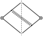
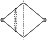
Figure 2: Diagrams contributing to the one-loop soft function.

For a generic angularity one obtains in Laplace space

$$\hat{\cal S}_{\rm bare}(\mu,\nu)=1 +\frac{\alpha_{s}(\mu)}{\pi}C_{F}\left[\frac{1}{\epsilon^{2}}+\frac{2}{\epsilon}\ln\frac{\mu}{\nu}\right.$$

$$\left.+\frac{1}{2-a}\left(2(1-a)\ln^{2}\frac{\mu}{\nu}-2\ln^{2}\frac{\mu u}{Qu_{0}}+4\ln\frac{\mu}{\nu}\ln\frac{\mu u}{Qu_{0}}-\frac{\pi^{2}}{12}(2+3a)\right)\right]\,.$$ (99)

The soft anomalous dimensions are then extracted using Eq. (58) and (68), which at one loop give

$$\gamma^{(\mu)}_{S}(\mu,\nu)= \,4\frac{\alpha_{s}(\mu)}{\pi}C_{F}\ln\frac{\mu}{\nu}+{\cal O}(\alpha_{s}^{2})\,,$$

$$\gamma^{(\nu)}_{1,1-a;S}(\mu,\nu)= -4\frac{\alpha_{s}(\mu)}{\pi}C_{F}\ln\frac{\mu}{\mu(\nu)}+{\cal O}(\alpha_{s}^{2})\,.$$ (100)

This verifies Eqs. (4.2) and (4.2) to ${\cal O}(\alpha_{s})$ and gives the well known results $\Gamma_{\rm cusp}^{(0)}=4C_{F}$,

$$\widehat{\gamma}^{(0)}_{S}[\alpha_{s}(\mu)]=0\,,$$ (101)

and

$$\qquad\gamma_{1,1-a}^{(\nu,\,0)}[\alpha_{s}(\mu)]=0\,.$$ (102)

Similarly, the zero-bin subtracted one-loop jet function is given by all possible cuts of the diagrams shown in Fig. 3.

Figure 3: Diagrams contributing to the one-loop jet function. The jet function is given by the sum over all cuts.

After performing the zero-bin subtraction, which becomes non-trivial in the presence of the extra UV regulator, we get

$$\hat{\cal J}_{n,{\rm bare}}(\mu,\nu)=1 +\frac{\alpha_{s}(\mu)}{\pi}C_{F}\bigg{\{}\frac{3}{4\epsilon}+\frac{\ln\frac{\nu}{Q}}{\epsilon}$$

$$+\frac{1}{2-a}\left[\ln\left(\frac{\mu}{Q}\left(\frac{u}{u_{0}}\right)^{\frac{1}{2-a}}\right)\left(3-\frac{3}{2}a+2(2-a)\ln\frac{\nu}{Q}\right)-(1-a)\ln^{2}\frac{\nu}{Q}\right.$$

$$\left.\,+\frac{1}{12}\left(60-39a+\pi^{2}(6a-8)-18\ln 2\right)\right]\bigg{\}}\,,$$ (103)

from which we obtain the one loop anomalous dimensions of the jet function

$$\gamma^{(\mu)}_{J}(\mu,\nu) =\frac{\alpha_{s}(\mu)}{\pi}C_{F}\left(2\ln\frac{\nu}{Q}+\frac{3}{2}\right)+{\cal O}(\alpha_{s}^{2}),\quad$$

$$\gamma^{(\nu)}_{1,1-a;J}(\mu,\nu) =\,2\frac{\alpha_{s}(\mu)}{\pi}C_{F}\ln\frac{\mu}{\mu(\nu)}+{\cal O}(\alpha_{s}^{2})\,.$$ (104)

One therefore confirms Eq. (102) and obtains

$$\widehat{\gamma}^{(0)}_{J}[\alpha_{s}(\mu)] =6\,C_{F}\,.$$ (105)

Note that at one-loop order the $\nu$ anomalous dimension is independent of the observable since $\gamma_{1,1-a}^{(\nu,\,0)}=0$. It is necessary to go to two loop order in order to analyze its observable dependence.

6.2 Two loop result

We now describe the main steps of the two loop calculation of the soft anomalous dimensions, while the jet anomalous dimensions can be derived via consistency relations by requiring the physical distribution of the angularities to be both $\mu$ and $\nu$ independent. The relevant Feynman diagrams are given in Fig. 4, where the mirror conjugate graphs have been omitted for simplicity.

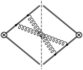
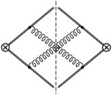
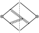
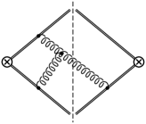
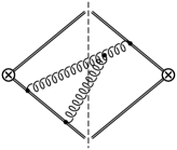
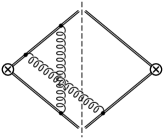
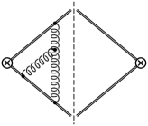
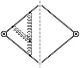
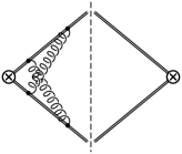
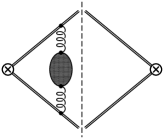
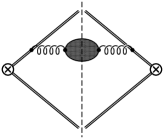
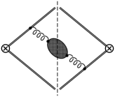
Figure 4: Diagrams contributing to the non-Abelian part of the two-loop soft function. The gray blobs include the contribution of quarks, gluons and ghosts to the self energy of the gluon.

We start from the standard Sudakov decomposition for the two soft partons $k_{a}$ and $k_{b}$,

$$k_{a}^{\mu} =k_{a}^{-}\frac{n^{\mu}}{2}+k_{a}^{+}\frac{\bar{n}^{\mu}}{2}+k^{\mu}_{a,t}\,,$$

$$k_{b}^{\mu} =k_{b}^{-}\frac{n^{\mu}}{2}+k_{b}^{+}\frac{\bar{n}^{\mu}}{2}+k^{\mu}_{b,t}\,,$$ (106)

with $k_{i}^{+}=n\cdot k_{i}$, $k_{i}^{-}=\bar{n}\cdot k_{i}$, and $n\cdot\bar{n}=2$. We also define $k_{i,\perp}^{2}=-k_{i,t}^{2}$ and $k_{i}^{+}k_{i}^{-}=k_{i,\perp}^{2}$. The double virtual diagrams give a scaleless contribution. For the real-virtual corrections, the one-loop amplitude for the emission of a soft gluon was derived in Catani:2000pi , and the phase space of the real gluon is parameterized as

$$\frac{{\rm d}^{d}k_{a}}{(2\pi)^{d-1}}\,\delta(k_{a}^{2})\,\Theta(k_{a}^{0})=\frac{1}{2}{\rm d}k_{a}^{+}\,{\rm d}k_{a}^{-}\,\frac{{\rm d}^{2-2\epsilon}k_{a,t}}{(2\pi)^{3-2\epsilon}}\,\delta(k_{a}^{+}k_{a}^{-}-k_{a,\perp}^{2})\,.$$ (107)

For the double real correction, we introduce the variable $z$ as

$$k_{a}^{-}=zk^{-},\quad k_{b}^{-}=(1-z)k^{-}\,,$$ (108)

where $k^{\pm}$ are the light cone components of the $k^{\mu}\equiv k_{a}^{\mu}+k_{b}^{\mu}$ momentum of invariant mass $m$ and now

$$k^{+}k^{-}=k_{\perp}^{2}+m^{2}\,.$$ (109)

The $d$-dimensional phase space for the emission of $k_{a}$ and $k_{b}$ can then be parameterized as

$$[{\rm d}k_{ab}] \equiv\frac{{\rm d}^{d}k_{a}}{(2\pi)^{d-1}}\frac{{\rm d}^{d}k_{b}}{(2\pi)^{d-1}}\,\delta(k_{a}^{2})\,\Theta(k_{a}^{0})\,\delta(k_{b}^{2})\Theta(k_{b}^{0})$$

$$=\frac{1}{2}{\rm d}k^{+}{\rm d}k^{-}\frac{{\rm d}^{2-2\epsilon}k_{t}}{(2\pi)^{3-2\epsilon}}\frac{{\rm d}m^{2}}{m^{2\epsilon}}\delta(k^{+}k^{-}-k_{\perp}^{2}-m^{2})\frac{1}{(4\pi)^{2}}\,{\rm d}z\,z^{-\epsilon}(1-z)^{-\epsilon}\frac{{\rm d}\Omega_{2-2\epsilon}}{(2\pi)^{1-2\epsilon}}\,,$$ (110)

with $\Omega_{2-2\epsilon}$ being the $(2-2\epsilon)$-dimensional solid angle

$$\frac{{\rm d}\Omega_{2-2\epsilon}}{(2\pi)^{1-2\epsilon}}=\frac{(4\pi)^{\epsilon}}{\sqrt{\pi}\Gamma\left(\frac{1}{2}-\epsilon\right)}{\rm d}\phi\sin^{-2\epsilon}\phi\,.$$ (111)

The $C_{F}C_{A}$ and $C_{F}n_{F}$ contributions to the double soft, tree-level squared amplitude (hereby denoted by $M^{2}_{s,0}(k_{a},k_{b})$) can be found in several places and it is given in the above parameterization in Appendix A. Due to the non-Abelian exponentiation theorem Gatheral:1983cz ; Frenkel:1984pz , we do not consider the $C_{F}^{2}$ contribution from the radiation of two independent gluons off the Wilson lines, as that is determined entirely by the leading order calculation given in the previous subsection and hence does not contribute to the two-loop soft anomalous dimension.

For a given angularity $\tau_{a}(k_{a},k_{b})$ evaluated on a double real final state $\{k_{a},k_{b}\}$, we then organize the calculation as follows:

• We express the value of the angularity $\tau_{a}(k_{a},k_{b})$ in terms of the above phase space variables as

  $$\tau_{a}(k_{a},k_{b}) =\,\frac{k_{\perp}}{Q}e^{-(1-a)|\eta|}\,(1+\mu^{2})^{\frac{a-1}{2}}\,f_{a}(z,\mu,\phi)\,,$$

  $$f_{a}(z,\mu,\phi) =\Bigg{[}z\bigg{(}1+2\sqrt{\frac{1-z}{z}}\mu\cos\phi+\frac{1-z}{z}\mu^{2}\bigg{)}^{1-\frac{a}{2}}$$

  $$\qquad+(1-z)\bigg{(}1-2\sqrt{\frac{z}{1-z}}\mu\cos\phi+\frac{z}{1-z}\mu^{2}\bigg{)}^{1-\frac{a}{2}}\Bigg{]}\,,$$ (112)

  where $\mu^{2}\equiv m^{2}/k_{\perp}^{2}$ and $\eta=\frac{1}{2}\ln\frac{k^{-}}{k^{+}}$.

• We split the double-real correction into two terms as follows

  $${\cal I}_{RR} \equiv\frac{1}{2}\int[{\rm d}k_{ab}]\,e^{-(k^{+}+k^{-})\frac{e^{-\gamma_{E}}}{\nu}}\,M^{2}_{s,0}(k_{a},k_{b})\,\delta(\tau-\tau_{a}(k_{a},k_{b}))={\cal I}_{RR}^{\small\rm{(I)}}+{\cal I}_{RR}^{\small\rm{(NI)}}\,,$$ (113)

  where the factor $1/2$ in Eq. (113) is a combinatorial factor in the case of two gluons, and represents $T_{F}=1/2$ in the case of a gluon splitting into two quarks (factored out from the squared amplitude given in Appendix A). We introduce a simplified observable $\tilde{\tau}_{a}(k)$ defined as

  $$\tilde{\tau}_{a}(k)=\frac{k_{\perp}}{Q}e^{-(1-a)|\eta|}\,,$$ (114)

  with, as above, $\eta=\frac{1}{2}\ln\frac{k^{-}}{k^{+}}$. The double real contribution can then be split as the sum of the following two integrals

  $${\cal I}_{RR}^{\small\rm{(I)}} =\frac{1}{2}\int[{\rm d}k_{ab}]\,e^{-(k^{+}+k^{-})\frac{e^{-\gamma_{E}}}{\nu}}\,M^{2}_{s,0}(k_{a},k_{b})\,\delta(\tau-\tilde{\tau}_{a}(k))\,,$$ (115)

  $${\cal I}_{RR}^{\small\rm{(NI)}} =\frac{1}{2}\int[{\rm d}k_{ab}]\,e^{-(k^{+}+k^{-})\frac{e^{-\gamma_{E}}}{\nu}}\,M^{2}_{s,0}(k_{a},k_{b})\left[\delta(\tau-\tau_{a}(k_{a},k_{b}))-\delta(\tau-\tilde{\tau}_{a}(k))\right]\,,$$

  The inclusive integral ${\cal I}_{RR}^{\small\rm{(I)}}$ is defined by the first equation in (115), that is replacing the angularity with the observable $\tilde{\tau}_{a}$. The non-inclusive correction ${\cal I}_{RR}^{\small\rm{(NI)}}$, defined by the second equation in (115), accounts for the difference between the actual observable $\tau_{a}(k_{a},k_{b})$ and its inclusive approximation $\tilde{\tau}_{a}(k)$.

The reason for splitting the calculation into an inclusive and non-inclusive contribution is that, as discussed in this paper, ${\cal I}_{RR}^{\small\rm{(NI)}}$ encodes the difference between two IRC safe observables which only depends on the extra UV regulator, but is finite in dimensional regularization and does not contribute to the $\widehat{\gamma}_{S}[\alpha_{s}(\mu)]$ anomalous dimension. Therefore this non-inclusive piece, which contains the complexity associated with the observable definition, is defined solely in terms of double real diagrams and can be evaluated directly in four dimensions (numerically if necessary). Similar ideas were proposed and exploited in Refs. Jouttenus:2011wh ; Bauer:2011hj ; Banfi:2014sua ; Gangal:2016kuo . Conversely, the inclusive contribution is considerably simpler and can be easily computed analytically for a generic observable. The $\gamma_{1,1-a}^{(\nu)}[\alpha_{s}(\mu)]$ anomalous dimension governing the $\nu$ RGE receives contributions from both integrals. We recall that, in general, one should take the limit $\epsilon\to 0$ first, in order to isolate the observable dependence with the $\nu$ exponential regulator. An exception is given by the case $a=1$ (broadening-like angularity), where the two limits $\epsilon\to 0$ and $\nu\to\infty$ commute with the regulator adopted here.

Working in the $\overline{\rm MS}$ scheme, we obtain the following two-loop anomalous dimensions

$$\widehat{\gamma}^{(1)}_{S}[\alpha_{s}(\mu)] =\,2\,C_{F}C_{A}\left(\frac{808}{27}-\frac{11}{9}\pi^{2}-28\zeta_{3}\right)-2\,C_{F}n_{F}T_{F}\left(\frac{224}{27}-\frac{4}{9}\pi^{2}\right)$$

$$=\,2\,C_{F}C_{A}\left(\frac{808}{27}-28\zeta_{3}\right)-2\,C_{F}n_{F}T_{F}\frac{224}{27}-\frac{2}{3}\pi^{2}C_{F}\,b_{0}\,,$$

$$\gamma_{1,1-a}^{(\nu,\,1)}[\alpha_{s}(\mu)] =-\,C_{F}C_{A}\left(\frac{808}{27}-28\zeta_{3}\right)+\,C_{F}n_{F}T_{F}\frac{224}{27}-\frac{4}{3}\pi^{2}C_{F}\frac{2-a(2-a)}{(2-a)^{2}}\,b_{0}$$

$$\quad-16C_{F}\left(C_{A}\gamma_{a}^{(C_{A})}+T_{F}n_{F}\gamma_{a}^{(n_{F})}\right)\,,$$ (116)

with $b_{0}=({11C_{A}-2n_{F}})/{3}$. In the computation we expanded the part of the exponential function in the integrand relative to the smaller light cone component, and neglect subleading power corrections that would not contribute to the (leading power) anomalous dimensions. The inclusive contribution was evaluated analytically using sector decomposition with the help of HypExp Huber:2005yg , and cross checked numerically with pySecDec Borowka:2017idc . The quantities $\gamma_{a}^{(C_{A})}$ and $\gamma_{a}^{(n_{F})}$ arise from the non-inclusive correction which can be calculated in four dimensions. They are given by the finite integrals

$$\gamma_{a}^{(C_{A})} =\frac{1}{2-a}\int_{0}^{\infty}\frac{d\mu^{2}}{\mu^{2}(1+\mu^{2})}\int_{0}^{1}dz\int_{0}^{2\pi}\frac{d\phi}{2\pi}\frac{1}{2!}\left(2\mathcal{S}_{\rm s.o.}+\mathcal{H}_{g}\right)\ln f_{a}(z,\mu,\phi)\,,$$ (117)

$$\gamma_{a}^{(n_{F})} =\frac{1}{2-a}\int_{0}^{\infty}\frac{d\mu^{2}}{\mu^{2}(1+\mu^{2})}\int_{0}^{1}dz\int_{0}^{2\pi}\frac{d\phi}{2\pi}\mathcal{H}_{q}\ln f_{a}(z,\mu,\phi)\,,$$ (118)

where the functions ${\cal S}_{\rm s.o.}$, ${\cal H}_{g}$ and ${\cal H}_{q}$ are given in Appendix A, and the function $f_{a}$ is given in Eq. (• ‣ 6.2). A numerical computation shows that $\gamma_{a}^{(C_{A})}$, $\gamma_{a}^{(n_{F})}$ (for $a<2$) exhibit an almost exactly linear dependence on $a$, as displayed in Fig. 5. One can therefore expand these functions in a Taylor series around $a=0$, and consider the first few terms as an analytic approximation of the exact result. We evaluate the $\phi$ integrals by contour integration and, after integrating over $\mu$, we carry out the final integration over $z$ either analytically or numerically with ${\cal O}(100)$ significant digits, which allows us to reconstruct the analytic answer by means of the PSLQ algorithm 10.2307/2585116 . We also perform a numerical cross check using the Cuba libraries Hahn:2004fe . We give here the expansion to third order, which is sufficient to reach a few-permille accuracy in the interesting range $a\in[-1,1]$ considered in our study:

$$C_{A}\gamma_{a}^{(C_{A})}+T_{F}n_{F}\gamma_{a}^{(n_{F})}=-\frac{\zeta_{2}}{4}b_{0}+\left[C_{A}\left(\frac{41}{96}-\frac{\zeta_{2}}{4}-\frac{\zeta_{3}}{4}\right)-\frac{10}{96}T_{F}n_{F}\right]a$$

$$+\left[C_{A}\left(\frac{57\,941}{537\,600}+\frac{277}{163\,840}\zeta_{2}-\frac{9}{32}\zeta_{2}\,\ln 2+\frac{121}{640}\zeta_{3}\right)+T_{F}n_{F}\left(-\frac{131}{1440}+\frac{3}{40}\zeta_{3}\right)\right]a^{2}+{\cal O}(a^{3})\,.$$ (119)

The numerical value (i.e. not based on a Taylor expansion) for $\gamma_{a}^{(C_{A})}$, $\gamma_{a}^{(n_{F})}$ for $a<2$ is given in Table 1 for several values of $a$. The third order expansion of Eq. (6.2) provides an excellent approximation of the full result over the whole $a$ range relevant for the theoretical considerations made here on the transition between the SCET_I and SCET_II regimes, as can be seen from the comparison in Fig. 5.

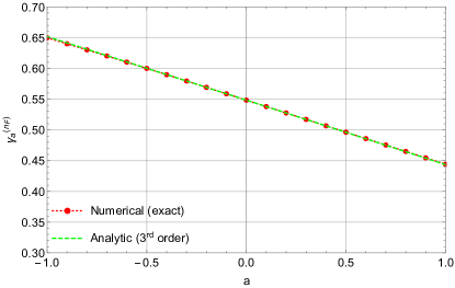
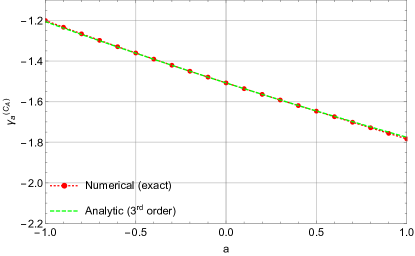
Figure 5: The functions $\gamma_{a}^{(n_{F})}$ (left) and $\gamma_{a}^{(C_{A})}$ (right) as a function of $a$. The dashed (green) line shows the analytic result based on a third order Taylor expansion, while the points (red) represent the result of the numerical integration.

$a$	$\gamma_{a}^{(n_{F})}$	$\gamma_{a}^{(C_{A})}$
-1.	0.650	-1.201
-0.9	0.640	-1.234
-0.8	0.630	-1.266
-0.7	0.620	-1.298
-0.6	0.610	-1.330
-0.5	0.600	-1.361
-0.4	0.590	-1.391
-0.3	0.579	-1.421
-0.2	0.569	-1.450
-0.1	0.559	-1.479

$a$	$\gamma_{a}^{(n_{F})}$	$\gamma_{a}^{(C_{A})}$
0.	0.548	-1.508
0.1	0.538	-1.536
0.2	0.527	-1.564
0.3	0.517	-1.592
0.4	0.507	-1.620
0.5	0.496	-1.647
0.6	0.486	-1.674
0.7	0.475	-1.701
0.8	0.465	-1.729
0.9	0.454	-1.756

$a$	$\gamma_{a}^{(n_{F})}$	$\gamma_{a}^{(C_{A})}$
1.	0.444	-1.784
1.1	0.434	-1.811
1.2	0.423	-1.839
1.3	0.413	-1.868
1.4	0.402	-1.896
1.5	0.392	-1.925
1.6	0.381	-1.955
1.7	0.371	-1.984
1.8	0.361	-2.015
1.9	0.350	-2.046

Table 1: Full numerical values for the functions $\gamma_{a}^{(n_{F})}$ and $\gamma_{a}^{(C_{A})}$ for different angularities corresponding to the parameter $a$, contributing to the soft anomalous dimensions of Eq. (6.2). The values for $\gamma_{a}^{(n_{F})}$ are rounded to the nearest 0.001, while for $\gamma_{a}^{(C_{A})}$ the numerical uncertainty is at most $\pm 1$ in the last digit.

As advertised, $\widehat{\gamma}_{S}[\alpha_{s}(\mu)]$ now does not depend on the specific observable, and it is given by the single logarithmic part of the soft anomalous dimension of the quark form factor, which coincides with the DGLAP soft anomalous dimension used for threshold resummation. Conversely, the entire observable dependence is now encoded in $\gamma_{1,1-a}^{(\nu)}$, which is common to the soft and jet functions and technically simpler to compute in that it only depends on the soft and collinear limit encoded in the zero-bin subtraction as discussed in Section 5.1. The corresponding anomalous dimensions for the jet function can be immediately derived from the standard consistency relation

$$\widehat{\gamma}^{(\mu)}_{S}[\alpha_{s}(\mu)]+2\,\widehat{\gamma}^{(\mu)}_{J}[\alpha_{s}(\mu)]+\gamma_{H}[\alpha_{s}(\mu)]=0\,,$$ (120)

and from Eq. (4.2). In the next section we will show how to obtain the anomalous dimensions in standard SCET_I starting from the results obtained above using the considerations of Section 4.

6.3 Relation to standard SCET_I anomalous dimensions

While for $a=1$ the results of the previous section directly provide the standard SCET_II soft anomalous dimension, they can also be used to derive the SCET_I soft anomalous dimension as obtained in pure dimensional regularization by means of Eqs. (5.1). Analogous considerations hold for the jet function, therefore we focus on the soft function first.

The quantities $\widehat{\gamma}_{S}[\alpha_{s}(\mu)]$ and $\gamma_{1,1-a}^{(\nu)}[\alpha_{s}(\mu)]$ entering Eqs. (5.1) are given in Eq. (6.2), and the only missing quantity is the one-loop coefficient $d_{1,1-a}^{(1)}$ of the initial condition of the $\Delta_{1,1-a}$ function (cf. Eq. (5.1)). This can be determined either by taking the square root of the ratio between the initial condition (constant part) of the one-loop soft function (6.1) and the corresponding result in pure dimensional regularization, or equivalently by calculating the zero-bin subtraction and taking its constant part. The one-loop soft function in dimensional regularization can be found in Ref. Fleming:2007xt , and its initial condition in Laplace space reads

$$\hat{\cal S}^{\rm SCET_{I}}(\mu=M_{S})=1-\frac{\alpha_{s}(\mu_{S})}{4\pi}\frac{\pi^{2}}{1-a}C_{F}\,.$$ (121)

Taking the square root of the ratio of the constant part of Eq. (6.1) to the latter equation we obtain

$$d_{1,1-a}^{(1)}=\frac{\pi^{2}}{6}C_{F}\frac{4+a(3a-4)}{(2-a)(1-a)}\,.$$ (122)

We set $\alpha=1$ and $\beta=1-a$ in Eqs. (5.1), and consider the series

$$\widehat{\gamma}^{\rm SCET_{I}}_{1,1-a;F}[(\alpha_{s}(\mu))]=\sum_{n=0}\left(\frac{\alpha_{s}(\mu)}{4\pi}\right)^{n+1}\widehat{\gamma}^{(n),\,{\rm SCET_{I}}}_{1,1-a;F}\,,$$ (123)

finding

$$\widehat{\gamma}^{(0),\,{\rm SCET_{I}}}_{1,1-a;S} =0\,,$$

$$\widehat{\gamma}^{(1),\,{\rm SCET_{I}}}_{1,1-a;S} =\frac{1}{1-a}\bigg{[}-2\,C_{F}C_{A}\left(\frac{808}{27}-28\zeta_{3}\right)+\,2C_{F}T_{F}n_{F}\frac{224}{27}+\frac{2}{3}\pi^{2}C_{F}(2a-3)b_{0}$$

$$\quad-32(2-a)C_{F}\left(C_{A}\gamma_{a}^{(C_{A})}+T_{F}n_{F}\gamma_{a}^{(n_{F})}\right)\bigg{]}\,,$$ (124)

where an analytic approximation of $\gamma_{a}^{(C_{A})}$ and $\gamma_{a}^{(n_{F})}$ is given in Eq. (6.2) or, alternatively, their numerical value is reported in Table 1.

To check this result, we compare the second of Eqs. (6.3) to the result of Ref. Bell:2018vaa , where the soft function was computed numerically. In order to compare to Figure 1 of Ref. Bell:2018vaa , we consider the quantity

$$\frac{1-a}{2}\,\widehat{\gamma}^{(1),\,{\rm SCET_{I}}}_{1,1-a;S}\,,$$ (125)

and we show the result in Fig. 6, where we have used Table 1 for the constants $\gamma_{a}^{(C_{A})}$ and $\gamma_{a}^{(n_{F})}$. The result of Eq. (6.3) is given by the red dashed line, while the green triangles are the numerical result of Ref. Bell:2018vaa for selected values of the parameter $a$. The two results are in perfect agreement.

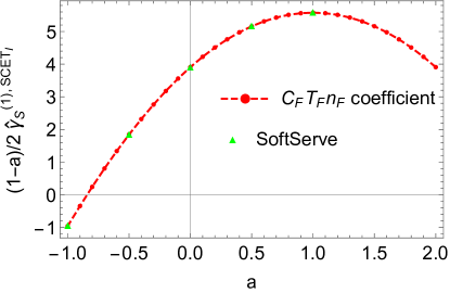
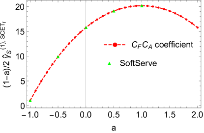
Figure 6: Soft anomalous dimension for angularities (multiplied by $(1-a)/2$) corresponding to the parameter $a$: coefficient of $T_{F}C_{F}n_{F}$ (left) and $C_{A}C_{F}$ (right) color factors.

As an additional check, we compare the NNLL resummed cross section (3) to the analytic formulae of Refs. Banfi:2014sua ; Banfi:2018mcq , reproducing the results given there. As a final check, for $a=0$ the result of Eq. (6.3) reproduces the soft anomalous dimension for thrust derived in Refs. Becher:2008cf ; Kelley:2011ng ; Monni:2011gb ; Hornig:2011iu . Analogous considerations can be used to derive the two loop jet anomalous dimension, that can be obtained by combining Eq. (5.1) and the consistency relation (120). Alternatively, it can be directly extracted from the soft anomalous dimension and the hard anomalous dimension (extracted from Refs. Matsuura:1987wt ; Matsuura:1988sm ; Gehrmann:2005pd ; Moch:2005id ; Becher:2006mr ), by imposing that the cross section is independent of the unphysical scales $\mu$ and $\nu$. We obtain

$$\widehat{\gamma}^{(1),\,{\rm SCET_{I}}}_{1,1-a;J} =C_{F}^{2}\left(3-4\pi^{2}+48\zeta_{3}\right)+\frac{C_{F}\,C_{A}}{1-a}\left(\frac{1769}{27}-80\zeta_{3}-\frac{961}{27}a-\frac{11}{9}\pi^{2}(5a-6)+52\zeta_{3}a\right)$$

$$\!\!\!-\frac{C_{F}\,n_{F}}{1-a}\left(\frac{242}{27}+\frac{4}{3}\pi^{2}-\frac{130}{27}a-\frac{10}{9}\pi^{2}a\right)+16\,\frac{2-a}{1-a}C_{F}\left(C_{A}\gamma_{a}^{(C_{A})}+T_{F}n_{F}\gamma_{a}^{(n_{F})}\right)\,.$$ (126)

6.4 Study of the $\nu$-regularization scheme dependence of $\gamma^{(\nu)}$

We finally wish to discuss the dependence of the soft and jet anomalous dimensions on the specific regularization scheme used to single out the UV divergences in the real radiation. In order to verify the validity of Eq. (96), we perform the calculation of the two loop soft anomalous dimensions discussed in the previous section using a different UV regularization scheme for the real radiation integrals. As an alternative to the exponential regulator, we simply impose a cutoff in the light cone component of the momentum of each real particle, that is the constraint

$$\Theta(\nu-\max\{k^{+},k^{-}\}),~{}\forall~{}{\rm real}~{}k\,.$$ (127)

The integrals in this scheme are similar to the full QCD case with soft amplitudes. Following the same procedure outlined in the previous section, we obtain

$$\widehat{\gamma}^{(1)}_{S}[\alpha_{s}(\mu)] =\,2\,C_{F}C_{A}\left(\frac{808}{27}-28\zeta_{3}\right)-2\,C_{F}n_{F}T_{F}\frac{224}{27}-\frac{2}{3}\pi^{2}C_{F}b_{0}\,,$$

$$\gamma_{1,1-a}^{(\nu,\,1)}[\alpha_{s}(\mu)] =-\,C_{F}C_{A}\left(\frac{808}{27}-28\zeta_{3}\right)+\,C_{F}n_{F}T_{F}\frac{224}{27}-\frac{4}{3}\pi^{2}C_{F}\frac{b_{0}}{(2-a)^{2}}$$

$$\quad-16C_{F}\left(C_{A}\gamma_{a}^{(C_{A})}+T_{F}n_{F}\gamma_{a}^{(n_{F})}\right)\,,$$ (128)

where $\gamma_{a}^{(C_{A})}$ and $\gamma_{a}^{(n_{F})}$ are the same as before. We see that $\widehat{\gamma}^{(1)}_{S}[\alpha_{s}(\mu)]$ is independent of the choice of the regulator as expected, while $\gamma_{1,1-a}^{(\nu,\,1)}[\alpha_{s}(\mu)]$ is regulator dependent and differs from Eq. (6.2). In order to connect the two results, we need the one loop coefficient $d_{1,1-a}^{(1)}$ that we can extract from the finite part of the renormalized one loop soft function in the light cone cutoff scheme, which reads

$$\hat{\cal S}(\mu,\nu)=1 +\frac{\alpha_{s}(\mu)}{\pi}C_{F}\left[\frac{1}{2-a}\left(2(1-a)\ln^{2}\frac{\mu}{\nu}+4\ln\frac{\mu}{\nu}\ln\frac{\mu u}{Qu_{0}}-2\ln^{2}\frac{\mu u}{Qu_{0}}-\frac{\pi^{2}}{12}(6-a)\right)\right]\,.$$ (129)

The coefficient $d_{1,1-a}^{(1)}$ is then obtained as the square root of the ratio of the constant term of the above soft function to the result in pure dimensional regularization (121), obtaining

$$d_{1,1-a}^{(1)}=\frac{\pi^{2}}{6}C_{F}\frac{a(4-a)}{(2-a)(1-a)}\,.$$ (130)

One can then verify that the quantity (96) evaluated at two loops, namely

$$\,\frac{2-a}{1-a}\,\gamma_{1,1-a}^{(\nu,\,1)}[\alpha_{s}(\mu)]-2\beta(\alpha_{s})\frac{{\rm d}\ln\Delta_{1,1-a}}{{\rm d}\alpha_{s}}\to{\rm\nu~{}scheme~{}invariant~{}in~{}SCET_{I}}\,,$$ (131)

is identical in the two schemes. This observation can be very useful in performing perturbative calculations for the anomalous dimensions. Specifically, one can carry out the computation semi-analytically in a scheme that is very suitable for a numerical evaluation (such as the light-cone cutoff scheme), and later convert the result into a scheme with better analytic properties such as boost invariance, as in the case of the exponential regulator.

One last comment concerns the constant terms of the two loop soft function in the extra UV regulator. These are unconstrained by theoretical arguments and only the combination of soft and jet functions is independent of the particular UV regularization scheme adopted in real radiation integrals.

7 Conclusions and Outlook

In this article we have studied the observable dependence of anomalous dimensions in SCET_I problems, and showed that the introduction of an extra UV regulator in real radiation integrals can be used to disentangle this dependence in perturbative calculations. The system of RGEs of the theory with the additional regulator shares many analogies with that of SCET_II problems in the formalism of the rapidity renormalization group. This connection highlights some similarities between the two theories. Notably, the whole observable dependence is encoded in a single anomalous dimension ruling the evolution in the new UV regularization scale $\nu$ (corresponding to the rapidity regularization scale in the SCET_II case), and in the definition of the initial and final scales of the RGE evolution. Unlike in the SCET_II case, however, the dependence of the new soft and jet functions on the extra UV regulator can be completely refactorized and shown to cancel in their combination, without leaving behind a factorization (collinear) anomaly like in SCET_II. The explicit cancellation of the $\nu$ dependence makes it natural to identify the source of the observable dependence in the anomalous dimensions with the eikonalized jet function that defines the zero-bin subtraction, which becomes non-trivial in the presence of the extra UV regulator.

We derived an all-order relation between the anomalous dimensions of the version of SCET_I with the extra UV regulator, and the standard SCET_I regulated in pure dimensional regularization. We verified this relation explicitly at 2-loop order for the family of recoil-free angularities in $e^{+}e^{-}$ defined with respect to the winner-take-all axis. In this context, we carried out a computation of the two loop soft anomalous dimension and show how to derive the standard SCET_I soft anomalous dimension from it. This results in new analytic expressions for the perturbative expansion of this quantity up to two-loop order. Comparing to previous numerical results from the literature we find perfect agreement. We also calculate the new jet functions at one-loop, while the two loop jet anomalous dimension can be extracted exclusively from consistency relations, hence providing all necessary ingredients to carry out the resummation for these observables up to NNLL.

An interesting observation is that the calculation is carried out in the same framework and regularization scheme for SCET_I and SCET_II theories, hence keeping track of the analogies and differences between the two limits. Previous work in the literature which explored the transition between the SCET_I and SCET_II regimes for angularities is that of Refs. Larkoski:2014uqa ; Bell:2018vaa . These papers study the anomalous dimension in the SCET_II case ($a=1$ in our notation) as a limiting case of the SCET_I anomalous dimension by exploiting the fact that the factorization theorem is continuous at the transition point. In this article we took an orthogonal point of view and formulated the resummation in SCET_I in a way that resembles that of the SCET_II case, which provides a useful viewpoint on the connection between the two effective theories.

Although we used angularities to illustrate the structure of the anomalous dimensions in the presence of the extra UV regulator, the considerations apply more broadly to any SCET_I observable defined through the particles’ final state momenta. In future work it will be interesting to explore further the structure of the zero-bin subtraction for SCET_I in the presence of the extra UV regulator, mainly in the context of multi-leg processes where our observation suggests that the observable dependence in the anomalous dimensions arises from a quantity that is diagonal in color space. Moreover, a proof of the cancellation of the $\nu$ dependence between the soft and collinear sectors at the operator level would be highly desirable. Finally, we stressed that the introduction of the extra UV regulator makes real radiation integrals UV finite, and therefore makes the effective theory suitable for numerical calculations. A practical advantage of this observation is that the complicated observable dependence can be separated out from the renormalization procedure. As a result, the observable dependence of the anomalous dimensions is to a large extent isolated into finite integrals which can be also evaluated numerically. An alternative avenue to exploit this fact is via the numerical resummation algorithm presented in Ref. Bauer:2018svx ; Bauer:2019bsp .

Appendix A Double soft squared amplitude

In terms of the variables introduced in Section 6, the double soft tree-level squared matrix element reads

$$M_{s,0}^{2}(k_{a},k_{b})=(4\pi\alpha_{s}\mu^{2\epsilon})^{2}\frac{8C_{F}}{m^{2}(m^{2}+k_{t}^{2})}C_{ab}(k_{a},k_{b})\,,$$ (132)

where

$$C_{ab}(k_{a},k_{b})=C_{A}(2\mathcal{S}_{\rm s.o.}+\mathcal{H}_{g})+n_{f}\mathcal{H}_{q}\,.$$ (133)

The contribution due to two final-state quarks in Eq. (133) has been multiplied by two, to compensate for the overall $1/2$ factor in Eq. (115). The three functions $\mathcal{S}_{\rm s.o.}$, $\mathcal{H}_{g}$ and $\mathcal{H}_{q}$ are the $4-2\epsilon$-dimensional counterparts of the homonymous terms defined in Ref. Dokshitzer:1997iz and they are taken from Ref. Banfi:2018mcq . They depend only on the dimensionless variables $z$, $\phi$ and $\mu^{2}\equiv m^{2}/k_{t}^{2}$. It is also useful to introduce the rescaled momenta $\vec{u}_{i}=\vec{q}_{i}/k_{t}$, such that

$$u_{a}^{2}=1+2\sqrt{\frac{1-z}{z}}\mu\cos\phi+\frac{1-z}{z}\mu^{2}\,,\qquad u_{b}^{2}=1-2\sqrt{\frac{z}{1-z}}\mu\cos\phi+\frac{z}{1-z}\mu^{2}\,.$$ (134)

In terms of these variables, we have

$$2\mathcal{S}_{\rm s.o.} =\frac{1}{z(1-z)}\left[\frac{1-(1-z)\mu^{2}/z}{u_{a}^{2}}+\frac{1-z\mu^{2}/(1-z)}{u_{b}^{2}}\right]$$ (135a)

$$\mathcal{H}_{g} =-4+(1-\epsilon)\frac{z(1-z)}{1+\mu^{2}}\left(2\cos\phi+\frac{(1-2z)\mu}{\sqrt{z(1-z)}}\right)^{2}$$

$$+\frac{1}{2(1-z)}\left[1-\frac{1-(1-z)\mu^{2}/z}{u_{a}^{2}}\right]+\frac{1}{2z}\left[1-\frac{1-z\mu^{2}/(1-z)}{u_{b}^{2}}\right]$$ (135b)

$$\mathcal{H}_{q} =1-\frac{z(1-z)}{1+\mu^{2}}\left(2\cos\phi+\frac{(1-2z)\mu}{\sqrt{z(1-z)}}\right)^{2}\,.$$ (135c)

References

- (1) C. W. Bauer, S. Fleming and M. E. Luke, Summing Sudakov logarithms in in effective field theory, Phys. Rev. D 63 (2000) 014006, [hep-ph/0005275].
- (2) C. W. Bauer, S. Fleming, D. Pirjol and I. W. Stewart, An Effective field theory for collinear and soft gluons: Heavy to light decays, Phys. Rev. D 63 (2001) 114020, [hep-ph/0011336].
- (3) C. W. Bauer and I. W. Stewart, Invariant operators in collinear effective theory, Phys. Lett. B 516 (2001) 134–142, [hep-ph/0107001].
- (4) C. W. Bauer, D. Pirjol and I. W. Stewart, Soft collinear factorization in effective field theory, Phys. Rev. D 65 (2002) 054022, [hep-ph/0109045].
- (5) J.-y. Chiu, A. Jain, D. Neill and I. Z. Rothstein, The Rapidity Renormalization Group, Phys. Rev. Lett. 108 (2012) 151601, [1104.0881].
- (6) J.-Y. Chiu, A. Jain, D. Neill and I. Z. Rothstein, A Formalism for the Systematic Treatment of Rapidity Logarithms in Quantum Field Theory, JHEP 05 (2012) 084, [1202.0814].
- (7) T. Becher and M. Neubert, Drell-Yan Production at Small , Transverse Parton Distributions and the Collinear Anomaly, Eur. Phys. J. C 71 (2011) 1665, [1007.4005].
- (8) T. Becher, G. Bell and M. Neubert, Factorization and Resummation for Jet Broadening, Phys. Lett. B 704 (2011) 276–283, [1104.4108].
- (9) A. J. Larkoski, J. Thaler and W. J. Waalewijn, Gaining (Mutual) Information about Quark/Gluon Discrimination, JHEP 11 (2014) 129, [1408.3122].
- (10) C. F. Berger, T. Kucs and G. F. Sterman, Event shape / energy flow correlations, Phys. Rev. D 68 (2003) 014012, [hep-ph/0303051].
- (11) M. Dasgupta, F. A. Dreyer, K. Hamilton, P. F. Monni, G. P. Salam and G. Soyez, Parton showers beyond leading logarithmic accuracy, Phys. Rev. Lett. 125 (2020) 052002, [2002.11114].
- (12) F. A. Dreyer, G. P. Salam and G. Soyez, The Lund Jet Plane, JHEP 12 (2018) 064, [1807.04758].
- (13) C. W. Bauer, S. P. Fleming, C. Lee and G. F. Sterman, Factorization of Event Shape Distributions with Hadronic Final States in Soft Collinear Effective Theory, Phys. Rev. D 78 (2008) 034027, [0801.4569].
- (14) A. Hornig, C. Lee and G. Ovanesyan, Effective Predictions of Event Shapes: Factorized, Resummed, and Gapped Angularity Distributions, JHEP 05 (2009) 122, [0901.3780].
- (15) A. J. Larkoski, D. Neill and J. Thaler, Jet Shapes with the Broadening Axis, JHEP 04 (2014) 017, [1401.2158].
- (16) A. Banfi, B. K. El-Menoufi and P. F. Monni, The Sudakov radiator for jet observables and the soft physical coupling, JHEP 01 (2019) 083, [1807.11487].
- (17) G. Bell, A. Hornig, C. Lee and J. Talbert, angularity distributions at NNLL′ accuracy, JHEP 01 (2019) 147, [1808.07867].
- (18) M. Procura, W. J. Waalewijn and L. Zeune, Joint resummation of two angularities at next-to-next-to-leading logarithmic order, JHEP 10 (2018) 098, [1806.10622].
- (19) Z.-B. Kang, K. Lee, X. Liu and F. Ringer, Soft drop groomed jet angularities at the LHC, Phys. Lett. B 793 (2019) 41–47, [1811.06983].
- (20) M. Beneke, A. Chapovsky, M. Diehl and T. Feldmann, Soft collinear effective theory and heavy to light currents beyond leading power, Nucl. Phys. B 643 (2002) 431–476, [hep-ph/0206152].
- (21) M. Beneke and T. Feldmann, Multipole expanded soft collinear effective theory with nonAbelian gauge symmetry, Phys. Lett. B 553 (2003) 267–276, [hep-ph/0211358].
- (22) Y. Li, D. Neill and H. X. Zhu, An Exponential Regulator for Rapidity Divergences, 1604.00392.
- (23) C. W. Bauer and P. F. Monni, A numerical formulation of resummation in effective field theory, JHEP 02 (2019) 185, [1803.07079].
- (24) C. W. Bauer and P. F. Monni, A formalism for the resummation of non-factorizable observables in SCET, JHEP 05 (2020) 005, [1906.11258].
- (25) A. V. Manohar, Deep inelastic scattering as using soft collinear effective theory, Phys. Rev. D 68 (2003) 114019, [hep-ph/0309176].
- (26) C. W. Bauer and A. V. Manohar, Shape function effects in and decays, Phys. Rev. D 70 (2004) 034024, [hep-ph/0312109].
- (27) J.-y. Chiu, A. Fuhrer, R. Kelley and A. V. Manohar, Factorization Structure of Gauge Theory Amplitudes and Application to Hard Scattering Processes at the LHC, Phys. Rev. D 80 (2009) 094013, [0909.0012].
- (28) R. Goerke and M. Luke, Power Counting and Modes in SCET, JHEP 02 (2018) 147, [1711.09136].
- (29) M. Inglis-Whalen, M. Luke and A. Spourdalakis, Rapidity Logarithms in SCET Without Modes, 2005.13063.
- (30) M. Beneke, Public lectures, 2005, http://theor.jinr.ru/ hq2005/Lectures/Beneke/Beneke-Dubna-05.pdf.
- (31) J.-y. Chiu, F. Golf, R. Kelley and A. V. Manohar, Electroweak Sudakov corrections using effective field theory, Phys. Rev. Lett. 100 (2008) 021802, [0709.2377].
- (32) J.-y. Chiu, F. Golf, R. Kelley and A. V. Manohar, Electroweak Corrections in High Energy Processes using Effective Field Theory, Phys. Rev. D 77 (2008) 053004, [0712.0396].
- (33) J.-y. Chiu, R. Kelley and A. V. Manohar, Electroweak Corrections using Effective Field Theory: Applications to the LHC, Phys. Rev. D 78 (2008) 073006, [0806.1240].
- (34) T. Becher, M. Neubert and D. Wilhelm, Electroweak Gauge-Boson Production at Small : Infrared Safety from the Collinear Anomaly, JHEP 02 (2012) 124, [1109.6027].
- (35) T. Becher and G. Bell, Analytic Regularization in Soft-Collinear Effective Theory, Phys. Lett. B 713 (2012) 41–46, [1112.3907].
- (36) A. V. Manohar and I. W. Stewart, The Zero-Bin and Mode Factorization in Quantum Field Theory, Phys. Rev. D 76 (2007) 074002, [hep-ph/0605001].
- (37) X.-d. Ji, J.-p. Ma and F. Yuan, QCD factorization for semi-inclusive deep-inelastic scattering at low transverse momentum, Phys. Rev. D 71 (2005) 034005, [hep-ph/0404183].
- (38) J.-y. Chiu, A. Fuhrer, A. H. Hoang, R. Kelley and A. V. Manohar, Soft-Collinear Factorization and Zero-Bin Subtractions, Phys. Rev. D 79 (2009) 053007, [0901.1332].
- (39) J. Collins, Foundations of perturbative QCD, vol. 32. Cambridge University Press, 11, 2013.
- (40) M. G. Echevarria, I. Scimemi and A. Vladimirov, Universal transverse momentum dependent soft function at NNLO, Phys. Rev. D 93 (2016) 054004, [1511.05590].
- (41) J. Chay and C. Kim, Consistent treatment of rapidity divergence in soft-collinear effective theory, 2008.00617.
- (42) M. Beneke, C. Bobeth and R. Szafron, Power-enhanced leading-logarithmic QED corrections to , JHEP 10 (2019) 232, [1908.07011].
- (43) M. Beneke, P. Böer, J.-N. Toelstede and K. K. Vos, QED factorization of non-leptonic decays, 2008.10615.
- (44) S. Catani and M. Grazzini, The soft gluon current at one loop order, Nucl. Phys. B 591 (2000) 435–454, [hep-ph/0007142].
- (45) J. Gatheral, Exponentiation of Eikonal Cross-sections in Nonabelian Gauge Theories, Phys. Lett. B 133 (1983) 90–94.
- (46) J. Frenkel and J. Taylor, Nonabelian Eikonal Exponentiation, Nucl. Phys. B 246 (1984) 231–245.
- (47) T. T. Jouttenus, I. W. Stewart, F. J. Tackmann and W. J. Waalewijn, The Soft Function for Exclusive N-Jet Production at Hadron Colliders, Phys. Rev. D 83 (2011) 114030, [1102.4344].
- (48) C. W. Bauer, N. D. Dunn and A. Hornig, Subtractions for SCET Soft Functions, 1102.4899.
- (49) A. Banfi, H. McAslan, P. F. Monni and G. Zanderighi, A general method for the resummation of event-shape distributions in annihilation, JHEP 05 (2015) 102, [1412.2126].
- (50) S. Gangal, J. R. Gaunt, M. Stahlhofen and F. J. Tackmann, Two-Loop Beam and Soft Functions for Rapidity-Dependent Jet Vetoes, JHEP 02 (2017) 026, [1608.01999].
- (51) T. Huber and D. Maitre, HypExp: A Mathematica package for expanding hypergeometric functions around integer-valued parameters, Comput. Phys. Commun. 175 (2006) 122–144, [hep-ph/0507094].
- (52) S. Borowka, G. Heinrich, S. Jahn, S. Jones, M. Kerner, J. Schlenk et al., pySecDec: a toolbox for the numerical evaluation of multi-scale integrals, Comput. Phys. Commun. 222 (2018) 313–326, [1703.09692].
- (53) H. R. P. Ferguson, D. H. Bailey and S. Arno, Analysis of pslq, an integer relation finding algorithm, Mathematics of Computation 68 (1999) 351–369.
- (54) T. Hahn, CUBA: A Library for multidimensional numerical integration, Comput. Phys. Commun. 168 (2005) 78–95, [hep-ph/0404043].
- (55) S. Fleming, A. H. Hoang, S. Mantry and I. W. Stewart, Top Jets in the Peak Region: Factorization Analysis with NLL Resummation, Phys. Rev. D 77 (2008) 114003, [0711.2079].
- (56) G. Bell, R. Rahn and J. Talbert, Two-loop anomalous dimensions of generic dijet soft functions, Nucl. Phys. B 936 (2018) 520–541, [1805.12414].
- (57) T. Becher and M. D. Schwartz, A precise determination of from LEP thrust data using effective field theory, JHEP 07 (2008) 034, [0803.0342].
- (58) R. Kelley, M. D. Schwartz, R. M. Schabinger and H. X. Zhu, The two-loop hemisphere soft function, Phys. Rev. D84 (2011) 045022, [1105.3676].
- (59) P. F. Monni, T. Gehrmann and G. Luisoni, Two-Loop Soft Corrections and Resummation of the Thrust Distribution in the Dijet Region, JHEP 08 (2011) 010, [1105.4560].
- (60) A. Hornig, C. Lee, I. W. Stewart, J. R. Walsh and S. Zuberi, Non-global Structure of the Dijet Soft Function, JHEP 08 (2011) 054, [1105.4628].
- (61) T. Matsuura and W. van Neerven, Second Order Logarithmic Corrections to the {Drell-Yan} Cross-section, Z. Phys. C 38 (1988) 623.
- (62) T. Matsuura, S. van der Marck and W. van Neerven, The Calculation of the Second Order Soft and Virtual Contributions to the Drell-Yan Cross-Section, Nucl. Phys. B 319 (1989) 570–622.
- (63) T. Gehrmann, T. Huber and D. Maitre, Two-loop quark and gluon form-factors in dimensional regularisation, Phys. Lett. B 622 (2005) 295–302, [hep-ph/0507061].
- (64) S. Moch, J. Vermaseren and A. Vogt, The Quark form-factor at higher orders, JHEP 08 (2005) 049, [hep-ph/0507039].
- (65) T. Becher, M. Neubert and B. D. Pecjak, Factorization and Momentum-Space Resummation in Deep-Inelastic Scattering, JHEP 01 (2007) 076, [hep-ph/0607228].
- (66) Y. L. Dokshitzer, A. Lucenti, G. Marchesini and G. Salam, Universality of 1/Q corrections to jet-shape observables rescued, Nucl. Phys. B 511 (1998) 396–418, [hep-ph/9707532].