Supersymmetry and Representation Theory in Low Dimensions

Mathew Calkins^a,b, S. James Gates, Jr.^c,d, and Caroline Klivans^c,e,f

^aGoogle Search,
111 8th Ave, New York, NY 10011, USA,
^bCourant Institute of Mathematical Sciences, New York University,
251 Mercer Street, New York, NY 10012, USA
^cBrown Theoretical Physics Center,
Box S, 340 Brook Street, Barus Hall, Providence, RI 02912, USA
^dDepartment of Physics, Brown University,
Box 1843, 182 Hope Street, Barus & Holley, Providence, RI 02912, USA
^eDivision of Applied Mathematics, Brown University,
182 George Street, Providence, RI 02906, USA
and
^fInstitute for Computational & Experimental Research in Mathematics, Brown University,
121 South Main Street Providence, RI 02903, USA

ABSTRACT

Beginning from a discussion of the known most fundamental dynamical structures of the Standard Model of physics, extended into the realms of mathematics and theory by the concept of “supersymmetry” or “SUSY,” an introduction to efforts to develop a complete representation theory is given. Techniques drawing from graph theory, coding theory, Coxeter Groups, Riemann surfaces, and computational approaches to the study of algebraic varieties are briefly highlighted as pathways for future exploration and progress.

PACS: 11.30.Pb, 12.60.Jv
Keywords: algorithms, off-shell, optimization, supermultiplets, supersymmetry

1 Supersymmetry and the Standard Model

As far as experiments in elementary particle physics reveal, the basic constituents of matter and interactions (i.e. forces excluding gravity) in our universe can be summarized in the list of particles shown in the table indicated in Fig.  (1.1).

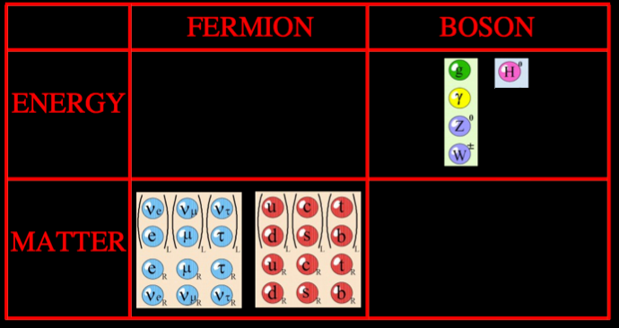
Figure 1.1: Diagrammatic Representation of the ‘Standard Model’ Particles

The matter particles consist of leptons and quarks shown in the lower left-hand quadrant. The most familiar member of the lepton family, shown within a light blue sphere, is the electron indicated by the letter “e.” The up and down quarks, indicated by the letters “u” and “d” surrounded by red spheres, are the most familiar of the quark family. They are also the principal constituents of protons and neutrons.

 The gauge or force-carrying particles appear in the upper right-hand quadrant. Each of the fundamental forces in nature is associated with one or more of these particles species. The strong nuclear force is associated with eight gluons indicated by the letter “g” within a green sphere. The electromagnetic force is associated with the photon indicated by the Greek letter “$\gamma$” within a yellow sphere. Finally, for the weak nuclear force the Higgs boson indicated by the letter “H” within a purple sphere, the Z-boson indicated by the letter “Z” within a dark blue sphere, and two charged W-bosons indicated by the symbols “$W^{+}$” and “$W^{-}$” also within dark blue spheres are the associated force-carrying particle species. The vertical heights of the quadrants of the elementary particles in Figure (1.1) thus corresponds to whether each particle is a carrier of a fundamental force (upper level) or is a matter particle (lower level) subject to such a force. How then is the left-right arrangement of the particles significant?

 One of the great discoveries of quantum mechanics is elementary particles (with the exception of the Higgs boson) all possess spin, a sort of intrinsic angular momentum which augments the particle’s more familiar orbital angular momentum. The rate of spin is constrained to take the form $n\,[h/(4\pi)]$, where $n$ is any nonnegative integer and $h$ is “Planck’s Constant,” a constant of nature empirically known to be roughly $6.626\times 10^{-34}$ Joules $\times$ seconds. If the integer $n$ associated with a specific particle is even the particle is called a ‘boson,’ if the integer is odd then the particle is called a ‘fermion.’ Thus, the left-right dichotomy shown in Figure (1.1) is due to grouping of all fermions to the left half and all bosons in right half of the diagram.

 As technology advances, additional elementary particles continue to be discovered, most recently with the 2012 initial observation of the Higgs boson. It is likely this trend will continue. One possibility for future discovery is indicated in Figure (1.2),

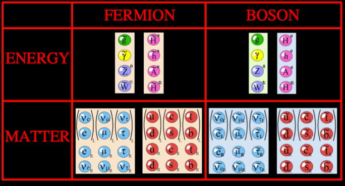
Figure 1.2: Diagrammatic Representation of the ‘Minimal SUSY Standard Model’ Particles

where a panoply of hypothetical new elementary particle species called superparticles (or more rarely sparticles) are shown. An easily noticeable feature of Figure (1.2), absent in Figure (1.1), is its left-right symmetry. This visual property is a reflection of a mathematical property called supersymmetry [1, 2] or SUSY. More formally, the possible states of a physics theory are elements of a Hilbert space. This includes the particles also described by such elements. A theory is said to possess supersymmetry if there exist linear maps $Q:\mathcal{H}\to\mathcal{H}$ (sometimes called supercharges) which take bosonic states to fermionic states and vice versa in a way that satisfies a certain algebra [1]. We will treat these ideas more carefully in a later section.

 Today’s experimentally confirmed particle theories do not feature supersymmetry. Supersymmetry generally requires the addition of new particle species as seen in Figure (1.2), so that the space of physical states and particles is closed under the action of each supercharge $Q$. However, there are many compelling reasons to suspect that supersymmetry (such as consistency of a quantum theory of gravitation), may be a feature of nature. Moreover by studying these speculative supersymmetric theories physicists have already extended knowledge about experimentally confirmed ones with greater precision.

2 Formal Aspects of Supersymmetry

2.1 Supersymmetry Field Theory

Supersymmetric quantum field theory is of interest to physicists for its role in theories of particle physics beyond the Standard Model [3, 4, 5] and of quantum gravity [6]. It has also borne fruit in pure mathematics, see e.g., [7]. The full story of SUSY QFT is complex and beyond the scope of this work, not the least because of the complexities of QFT in general, but the minimal version of the tale is as follows.

 Essentially all models of the physical universe consider the collection of all events, that is, ordered pairs $(ct,\mathbf{x})\equiv(x^{0},x^{1},x^{2},x^{3})$ of times and locations, as a smooth manifold aptly called spacetime^, In conventional QFT, we consider spacetime as it is modeled in the framework of special relativity: a real 4-dimensional affine space equipped with an inner product which, by judicious choice of coordinate system, can be put globally into the form

$$\eta(A,B):=A^{0}B^{0}-A^{1}B^{1}-A^{2}B^{2}-A^{3}B^{3}~{}~{}~{},$$ (1)

called the Minkowski metric for two such ordered pairs $(A^{0},A^{1},A^{2},A^{3})$ and $(B^{0},B^{1},B^{2},B^{3})$.

To make a long and subtle story very short, it turns out that the inner product is the core concept behind inertial reference frames: like any metric on any manifold, the numerical components of $\eta$ at any point in spacetime depend on the choice of local chart. Inertial reference frames are precisely those coordinate systems on spacetime in which the metric takes the above form at every point in the tangent space. Spacetime coordinate changes such as turning your head, hopping onto a steadily moving train, or adjusting your watch for Daylight Savings Time - are exactly those coordinate changes which preserve the form of the Minkowski metric, and which maintain the handedness of space and the direction of increasing time. Such changes are known as Poincaré transformations.

In order to reconcile these principles of special relativity with those of quantum mechanics, we consider the aforementioned Hilbert space acted upon by the Poincaré group of metric-preserving transformations, or more precisely by its corresponding algebra. In order to demonstrate the existence of representation of the Poincaré Lie algebra, a collection of operators $(P_{\mu})$ and $\left(M_{\mu\nu}\right)$, as well as their realization acting of the space of fields is introduced.

The physical states in the theory transform linearly in prescribed ways under the action of these generators, so that the classification of physical theories (before consideration of interactions) reduces to the classification of representations of the Poincaré algebra. This program is worked out in detail in [3] and [8] in language amenable to physicists and mathematicians, respectively. From this point of view, a physical theory is said to possess supersymmetry if there exist operators $\left(Q_{a}^{A}\right)$ in the spin representation of the Poincaré algebra which together with $\left(P_{\mu}\right)$ and $\left(M_{\mu\nu}\right)$ satisfy the SUSY algebra given in [1].

2.2 Supersymmetric mechanics

The story simplifies significantly if we project down to a spacetime with one temporal coordinate and no spatial coordinates (i.e., to the case of supersymmetric quantum mechanics).The Poincaré group of coordinate transformations then contains only translation along the time axis. This toy model features a collection of time-dependent bosonic fields $\phi_{i}(t)$ and fermionic fields $\psi_{i}(t)$ ($i=1,\ldots,d$), which are respectively even and odd in the sense that products of fields satisfy

$$\mbox{bosonic}\times\mbox{bosonic} =\mbox{bosonic}~{}~{}~{}\,~{}~{},$$

$$\mbox{bosonic}\times\mbox{fermionic} =\mbox{fermionic}~{}~{}~{},$$

$$\mbox{fermionic}\times\mbox{fermionic} =\mbox{bosonic}~{}~{}~{}\,~{}~{}.$$ (2)

The collection is known as a supermultiplet and the various fields its component fields.

 The component fields (and by extensions, derivatives and linear combinations thereof) are subject to the action of a collection of linear operators $Q_{\rm I}\ ({\rm I}=1,\ldots,\mathcal{N}$) called supercharges which are odd in the sense of mapping bosonic fields to fermionic fields and vice versa. The appropriately reduced SUSY algebra then demands only that the action of the supercharges on the component fields ought to satisfy relations involving $\partial_{0}$ (the infinitesimal generator of temporal translations) as shown below,

$$\{\,Q_{\rm I}~{},~{}Q_{\rm J}\,\}~{}=~{}i\,2\,\delta{}_{{\rm I}\,{\rm J}}\,\partial{}_{0}~{}~{}~{},$$ (3)

and

$$\left[\,Q_{\rm I}~{},~{}\partial{}_{0}\,\right]~{}=~{}0~{}~{}~{}.$$ (4)

If these relations are valid independent of any differential equations imposed on the fields, the supermultiplet together with the charges acting on it is said to be an off-shell representation of $N$-extended 1-dimensional supersymmetry. Since these relations constrain the ways the supercharges compose and add amongst themselves but say essentially nothing about the supermultiplet itself, we sometimes abuse vocabulary and refer to the supercharges alone as being such a representation.

 These 1-dimensional toy models offer a fertile ground for studying the general structure of supersymmetric representations, not the least because (as we shall discuss shortly) they allow the problem to be recast into combinatorial and graph-theoretic terms. This richness makes it possible to study more physically realistic higher-dimensional models of supersymmetry by projecting down to 1-dimensional models. Formally, this dimensional reduction starts with a system of supercharges acting on time- and space-dependent fields $\phi_{i}(t,\mathbf{x}),\psi_{j}(t,\mathbf{x})$ and modifies their actions by formally setting all derivatives with respect to the spatial coordinates to zero, leaving only derivatives (if any) with respect to time.

2.3 The Garden Algebra

In studying off-shell representations of $\mathcal{N}$-extended 1-dimensional supersymmetry, it is frequently useful to transform the component fields by invertible linear combinations

$${\phi_{i}\to\sum_{j=1}^{d}a_{ij}\phi_{j}~{}~{}~{},\ \ \ \psi_{i}\to\sum_{j=1}^{d}b_{ij}\psi_{j}\ \ \ (a_{ij},c_{ij}\in{\mathbb{C}})~{}~{}~{}~{}~{}~{},}$$ (5)

or by differentiation

$$\phi_{i}\to\left(\partial{}_{0}\right)^{c_{i}}\phi_{i}~{}~{}~{},\ \ \ \psi_{i}\to\left(\partial{}_{0}\right)^{d_{i}}\psi_{i}\ \ \ \left(c_{i},d_{i}\in\{0,1\}\right)~{}~{}~{},$$ (6)

both of which preserve satisfaction of the algebraic relations discussed above. Subject to some physically reasonable conditions discussed more thoroughly in [9], it is generally possible to perform a sequence of such transformations so that the actions of the supercharges take the off-diagonal form

$$Q_{\rm I}(\phi_{i})=\sum_{j=1}^{d}({\rm L}_{\rm I})_{ij}\psi_{j}~{}~{}~{},~{}~{}~{}\ \ \ Q_{\rm I}(\psi_{i})=i\sum_{j=1}^{d}({\rm R}_{\rm I})_{ij}\partial{}_{0}\phi_{j}~{}~{}~{}.$$ (7)

or equivalently

$$\begin{bmatrix}\phi_{1}\\ \vdots\\ \phi_{d}\\ \psi_{1}\\ \vdots\\ \psi_{d}\end{bmatrix}\xmapsto{Q_{\rm I}}\begin{bmatrix}0&{\rm L}_{\rm I}\\ i\,{\rm R}_{\rm I}\circ\partial{}_{0}&0\\ \end{bmatrix}\begin{bmatrix}\phi_{1}\\ \vdots\\ \phi_{d}\\ \psi_{1}\\ \vdots\\ \psi_{d}\end{bmatrix}~{}~{}~{}.$$ (8)

for some collection of matrices ${{\boldsymbol{{\rm L}}}}_{\rm I},{{\boldsymbol{{\rm R}}}}_{\rm I}\in Gl(n,\mathbb{R})$. In that case the condition $\{Q_{\rm I},Q_{\rm J}\}=2i\delta_{IJ}\partial{}_{0}$ reduces to the so-called Garden Algebra

$$\begin{split}{{\boldsymbol{{\rm L}}}}_{\rm I}\,{{\boldsymbol{{\rm R}}}}_{\rm J}~{}+~{}{{\boldsymbol{{\rm L}}}}_{\rm J}\,{{\boldsymbol{{\rm R}}}}_{\rm I}&~{}=~{}2\,\delta_{\rm{IJ}}\,\mathbf{1}~{}~{}~{},\\ {{\boldsymbol{{\rm R}}}}_{\rm I}\,{{\boldsymbol{{\rm L}}}}_{\rm J}~{}+~{}{{\boldsymbol{{\rm R}}}}_{\rm J}\,{{\boldsymbol{{\rm L}}}}_{\rm I}&~{}=~{}2\,\delta_{\rm{IJ}}\,\mathbf{1}~{}~{}~{},\end{split}$$ (9)

while the commutator relation $[Q_{\rm I}\,,\,\partial{}_{0}]=0$ holds automatically. Thus any collection of square matrices satisfying Eq. (9) furnishes a representation of off-shell $(\mathcal{N},d)$ supersymmetry. The matrices ${{\boldsymbol{{\rm L}}}}_{\rm I}$ and ${{\boldsymbol{{\rm R}}}}_{\rm I}$ (with the index ${\rm I}$ taking values of 1, $\dots$, $\mathcal{N}$) [10, 11] can also be used to construct $2d\times 2d$ matrices ${\widehat{{\boldsymbol{\gamma}}}}{}_{\rm I}$ [12] as

$${{\widehat{{\boldsymbol{\gamma}}}}{}_{\rm I}~{}=~{}\left[\begin{array}[]{cc}~{}0&~{}~{}{{\boldsymbol{{\rm L}}}}_{\rm I}\\ {}{}\hfil&{}\hfil\\ ~{}{{\boldsymbol{{\rm R}}}}_{\rm I}&~{}~{}0\\ \end{array}\right]~{}~{}~{},}$$ (10)

which form a Clifford Algebra, with respect to the Euclidean metric define by the Kronecker delta symbol $\delta_{\rm{IJ}}$

$$\left\{{\widehat{{\boldsymbol{\gamma}}}}{}_{\rm I},{\widehat{{\boldsymbol{\gamma}}}}{}_{\rm J}\right\}=2\delta_{\rm{IJ}}~{}~{}~{}.$$ (11)

3 The Adinkra Program - Supersymmetry from Decorated Graphs

Now we proceed with a pair of worked examples. We shall find that they admit a concise description not only in terms of matrices, but in terms of certain decorated graphs. We begin with a note on a historical accident of convention.

3.1 Charges and Derivatives

Thus far we have spoken of supersymmetric representations entirely in terms of the supercharges $Q_{\rm I}$. It turns out that supersymmetry can be reformulated into the geometric language of superspace [5], a sort of extension of spacetime to include fermionic coordinates in addition to the usual real bosonic coordinates. In this framework the supercharges become the generators of a certain group of translations in superspace. And just as coordinate changes on a real smooth manifold beg the notion of derivatives which are covariant with respect to those changes, superspace naturally motivates supercovariant derivatives $D_{\rm I}$ which are covariant with respect to those supertranslations. These derivatives satisfy the same algebra amongst themselves as the supercharges do, namely

$$\{\,D_{\rm I}~{},~{}D_{\rm J}\,\}~{}=~{}i\,2\,\delta{}_{{\rm I}\,{\rm J}}\,\partial{}_{0}~{}~{}~{},$$ (12)

and we can specify a supersymmetric system in terms of the action of these derivatives just as well as we can with the supercharges. In the relevant physics literature it is conventional to work largely in terms of the former, and for consistency with cited works we do the same here.

3.2 The Chiral and Vector Supermultiplets

After a healthy amount of theory and motivation we are ready to examine two concrete realizations of supersymmetry involving fields varying over both space and time [13]. The first example is the chiral supermultiplet:

$${\rm D}_{a}A~{} =~{}{\Psi}_{a}~{}~{}~{},~{}~{}~{}$$ (13)

$${\rm D}_{a}B~{} =~{}-\,i\,(\gamma^{5}){}_{a}{}^{b}\,{\Psi}_{b}~{}~{}~{},$$ (14)

$${\rm D}_{a}{\Psi}_{b}~{} =~{}i\,(\gamma^{\mu}){}_{a\,b}\,\partial_{\mu}A~{}+~{}(\gamma^{5}\gamma^{\mu}){}_{a\,b}\,\partial_{\mu}B~{}-~{}i\,C_{a\,b}\,F~{}+~{}(\gamma^{5}){}_{a\,b}G~{}~{},$$ (15)

$${\rm D}_{a}F~{} =~{}(\gamma^{\mu}){}_{a}{}^{b}\,\partial_{\mu}\,{\Psi}_{b}~{}~{}~{},~{}~{}~{}$$ (16)

$${\rm D}_{a}G~{} =~{}i\,(\gamma^{5}\gamma^{\mu}){}_{a}{}^{b}\,\partial_{\mu}\,{\Psi}_{b}~{}~{}~{}.$$ (17)

The second is the vector supermultiplet

$${\rm D}_{a}\,A{}_{\mu}~{} =~{}(\gamma_{\mu}){}_{a}{}^{b}\,{\lambda}_{b}~{}~{}~{},$$ (18)

$${\rm D}_{a}{\lambda}_{b}~{} =~{}-\,i\,\hbox{\large{${\frac{{1}}{{4}}}$}}([\,\gamma^{\mu}\,,\,\gamma^{\nu}\,]){}_{a}{}_{b}\,(\,\partial_{\mu}\,A{}_{\nu}~{}-~{}\partial_{\nu}\,A{}_{\mu}\,)~{}+~{}(\gamma^{5}){}_{a\,b}\,{\rm d}~{}~{},{~{}~{}~{}~{}~{}~{}~{}~{}~{}~{}}$$ (19)

$${\rm D}_{a}\,{\rm d}~{} =~{}i\,(\gamma^{5}\gamma^{\mu}){}_{a}{}^{b}\,\,\partial_{\mu}{\lambda}_{b}~{}~{}~{}.$$ (20)

A few notes on notation are due at this point. $A$, $B$, $F$ and $G$ are fields with spin $n$ = 0 much like the Higgs boson, $A{}_{\mu}$ has $n$ = 2, ${\Psi}_{a}$ and ${\lambda}_{a}$ are fields with $n$ = $1/2$, and $F,G$ and $d$ are auxiliary fields, which do not describe physically observable effects but are nonetheless necessary to maintain supersymmetry.

The $\gamma$ appearing in these equations are Dirac matrices, whose defining property is that they form a Clifford algebra with respect to the Minkowski metric.

$$\left\{\gamma^{\mu},\gamma^{\nu}\right\}=2\eta^{\mu\nu}\mathbb{I}~{}~{}~{}.$$ (21)

This condition alone does not fix the values of these matrices; we adopt the conventions in [14] for exact values of these matrices.

Greek letters - as in the $\mu$ which appears in several of the actions above - range from $0$ to $3$ and are used to index components of tensors over spacetime. The shorthand $\partial_{\mu}$ refers to the $\mu$-th component of the tuple $(\partial/\partial t,\partial/\partial x,\partial/\partial y,\partial/\partial z)\equiv(\partial/\partial x^{0},\partial/\partial x^{1},\partial/\partial x^{2},\partial/\partial x^{3})$. Latin indices early in the alphabet - $a$, $b$, $c$ above - are so-called spinor indices. They too indicate components of tensors and here range from 1 to 4. The term $(\gamma^{5})_{a}{}^{b}$, for example, is the $a,b$ component of the $4\times 4$ matrix $\gamma^{5}$. Both spacetime and spinor indices follow the Einstein summation convention, wherein any subscripted index paired with a superscripted matching one is taken to be summed over. For example,

$$-i\left(\gamma^{5}\right)_{a}{}^{b}\Psi_{b} \equiv-i\sum_{b=1}^{4}\left(\gamma^{5}\right)_{a}{}^{b}\Psi_{b}~{}~{}~{},$$ (22)

With notation established we can compute the action of $D_{1}$ on $B$ in the chiral supermultiplet. Following [14] we have

$$\gamma^{5}=\begin{pmatrix}0&0&0&i\\ 0&0&-i&0\\ 0&-i&0&0\\ i&0&0&0\end{pmatrix}~{}~{}~{},$$ (23)

and we find

$${\rm D}_{1}B=-i\left(\gamma^{5}\right)_{1}^{\ b}\Psi_{b}\equiv-i\sum_{b=1}^{4}\left(\gamma^{5}\right)_{1}^{\ b}\Psi_{b}=\Psi_{4}~{}~{}~{}.$$ (24)

As discussed earlier, we can produced a corresponding 1D version of the chiral supermultiplet by formally taking all derivatives $\partial_{\mu}$ - except for the time-derivative $\partial_{0}$ - to vanish. For example, the supercovariant derivative of the $F$ field in the chiral multiplet simplifies to

$${\rm D}_{a}F=\left(\gamma^{\mu}\right)_{a}^{\ b}\partial_{\mu}\Psi_{b}\ \to\ \left(\gamma^{0}\right)_{a}^{\ b}\partial_{0}\Psi_{b}~{}~{}~{}.$$ (25)

Again following [14],

$$\gamma^{0}=\begin{pmatrix}0&1&0&0\\ -1&0&0&0\\ 0&0&0&-1\\ 0&0&1&0\end{pmatrix}~{}~{}~{},$$ (26)

and from this we can read off the transformation laws for $F$ in the reduced version of the chiral multiplet.

$$\begin{cases}{\rm D}_{1}F&=\Psi_{2}\\ {\rm D}_{2}F&=-\Psi_{1}\\ {\rm D}_{3}F&=-\Psi_{4}\\ {\rm D}_{4}F&=\Psi_{3}\end{cases}~{}~{}~{}.$$ (27)

3.3 Adinkras

From the transformation laws Eq. (17, 20) above we see that the supercovariant derivatives in both multiplets take bosonic fields to linear combinations of fermionic fields (sometimes with time derivatives) and vice versa. But the calculations we’ve seen have taken an especially nice form. Rather then a general linear combination of fermions, each bosonic field has been taken to $\pm$ exactly one fermion Eq. (24, 27). Some further calculations with these multiplets show that each fermion goes to $\pm$ $i$ times just one corresponding boson! With this remarkable property we can build from each multiplet a decorated graph called an adinkra by the following procedure.

1. To each field in the multiplet we associate a node in the graph. Visually we represent bosonic and fermionic fields respectively with solid and open circles.

2. Whenever a transformation law takes one field to another, the corresponding nodes are connected by an edge. An edge coloring indicates which supercovariant derivative was involved. Multiplets like those given here are sometimes called four-color systems, and it is conventional to assign to $(\rm D_{1},\rm D_{2},\rm D_{3},\rm D_{4})$ some permutation of the colors (red, green, blue, black). An edge is drawn as a dashed line if the corresponding transformation law has a minus sign, and solid otherwise.

3. We arrange the nodes into horizontal rows, with one field appearing in the row directly above another if and only if there exists a transformation law taking the former to the time-derivative of the latter. For systems with corresponding ${{\boldsymbol{{\rm L}}}}$ and ${{\boldsymbol{{\rm R}}}}$ matrices, this forces the graph to take the form of a row of fermions sitting above a row of bosons.

Under this procedure, the dimensionally reduced chiral and vector supermultiplets map to the colorful images in Figure (3.1)

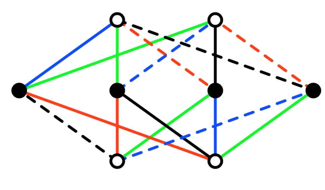
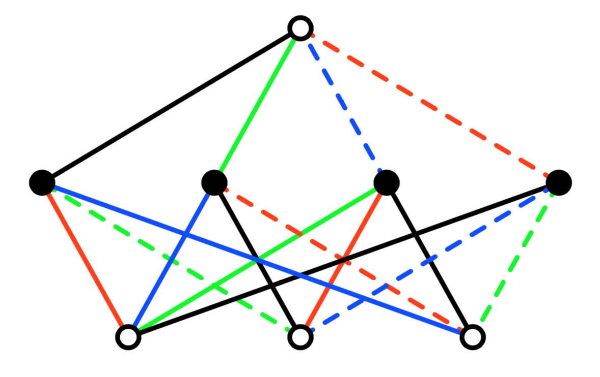
Figure 3.1: The Chiral and Vector Supermultiplets, Dimensionally Reduced and Converted to Adinkras

The Garden algebra realized on such representations then forces a number of regularities onto the graphs. For example, every node has exactly one adjacent edge of each color and any length-4 path along alternative colors forms a closed cycle with an odd number of dashed lines. Adinkras map interesting representation-theoretic properties to graph-theoretic ones, e.g., reducible representations correspond to disconnected adinkras. Perhaps most interestingly, Adinkras offer a direct means of constructing representations of 1D supersymmetry: take a collection of solid nodes, the same number of open nodes, arrange them into alternating rows, then connect them by colored edges with dashings as prescribed by certain combinatorial rules. Since the initiation of this line of thought in [15, 16], the adinkra program has extended from its roots in graph theory and supersymmetry into such languages of Riemann surfaces and Grothendieck “dessins d’ enfants,” [17, 18], and error correcting codes [19, 20, 21]. It also spurred novel approaches to the auxiliary field problem [22], described further in a later section.

4 The Adinkra Program - Enter A Coxeter Group

In the work of [23], the real $d\,\times\,d$ matrices that appear in Eq. (11) were explored computationally. The goal of this program was the explicit enumeration and construction of all linearly independent matrices that satisfy the condition in Eq. (11). The number of matrices found was 384 matrices. With a little “numerology” one realizes that 384 = 16 $\times$ 24 = $2^{4}$ $\times$ 4! and this is precisely the order of the Coxeter Group sometimes denoted by the moniker $BC{}_{4}$. An explicit examination of all the matrices revealed that each took a form given by

$${{\boldsymbol{{\rm L}}}}_{\,\widehat{{\rm I}}}~{}=~{}{{\boldsymbol{\cal S}}}_{\,\widehat{{\rm I}}}\,{{\boldsymbol{\cal P}}}_{\,\widehat{{\rm I}}}~{}~{}~{},$$ (28)

where the index ${\,\widehat{{\rm I}}}$ takes on values 1, 2, $\dots$, 384. Each of the matrices ${{\boldsymbol{\cal S}}}_{\,\widehat{{\rm I}}}$, for fixed value of ${\,\widehat{{\rm I}}}$, takes the form of a purely diagonal matrix with either plus one or minus one in each of the diagonal entries.

Similarly, for each of the matrices ${{\boldsymbol{\cal P}}}_{\,\widehat{{\rm I}}}$, for a fixed value of ${\,\widehat{{\rm I}}}$, takes the form of one of the elements in the permutation group of four elements. However, in order to satisfy the condition in Eq. (11), it was found that the entirety of the permutation group is disaggregated into six distinct unordered subsets referred to as “quartets”:

$$\begin{array}[]{ccc}~{}{{\boldsymbol{\{{\cal P}{}_{[1]}\}}}}&{{\boldsymbol{\equiv}}}&~{}~{}{{\boldsymbol{\{\,(123),\,(134),\,(142),\,(243)\,\}}}}~{}~{}~{},\\ }{}{\hfil&}{}{\hfil&\\ ~{}{{\boldsymbol{\{{\cal P}{}_{[2]}\}}}}&{{\boldsymbol{\equiv}}}&~{}~{}{{\boldsymbol{\{\,(124),\,(132),\,(143)\,,(234)\,\}}}}~{}~{}~{},\\ }{}{\hfil&}{}{\hfil&\\ ~{}{{\boldsymbol{\{{\cal P}{}_{[3]}\}}}}&{{\boldsymbol{\equiv}}}&~{}~{}{{\boldsymbol{\{\,(14),\,(23),\,(1243),\,(1342)\,\}}}}~{}~{}~{},\\ }{}{\hfil&}{}{\hfil&\\ ~{}{{\boldsymbol{\{{\cal P}{}_{[4]}\}}}}&{{\boldsymbol{\equiv}}}&~{}~{}{{\boldsymbol{\{(13),\,(24),\,(1234),\,\,(1432)\,\}}}}~{}~{}~{},\\ }{}{\hfil&}{}{\hfil&\\ ~{}{{\boldsymbol{\{{\cal P}{}_{[5]}\}}}}&{{\boldsymbol{\equiv}}}&~{}~{}{{\boldsymbol{\{\,(12),\,(34),\,(1324),\,(1423)\,\}}}}~{}~{}~{},\\ }{}{\hfil&}{}{\hfil&\\ ~{}{{\boldsymbol{\{{\cal P}{}_{[6]}\}}}}&{{\boldsymbol{\equiv}}}&~{}~{}{{\boldsymbol{\{\,(),\,(12)(34),\,(13)(24),\,(14)(23)\,\}}}}~{}~{}~{}.\end{array}$$ (29)

Stated another way, if one makes an arbitrary choice among the matrices in Eq. (28) and considers only its dependence on the permutation matrix that appears, the remaining three permutation elements must be in the same subset that is shown in Eq. (29) in order for the collection to satisfy Eq. (11).

There was one other property noted in [23] about this disaggregation. The concept of Hodge Duality of forms is well established in differential geometry. Essentially, an operation was uncovered on the collection of disaggregated quartets that “shadows” the four dimensional Hodge Duality acting on the supermultiplets of field variables.

$$\begin{array}[]{r@{\>=\>}l}{}^{{\boldsymbol{*}}}\{{{\boldsymbol{\cal P}}{}_{[1]}}\}&\{{{\boldsymbol{\cal P}}{}_{[2]}}\}~{},\\ {}^{{\boldsymbol{*}}}\{{{\boldsymbol{\cal P}}{}_{[2]}}\}&\{{{\boldsymbol{\cal P}}{}_{[1]}}\}~{},\\ \end{array}\qquad\begin{array}[]{r@{\>=\>}l}{}^{{\boldsymbol{*}}}\{{{\boldsymbol{\cal P}}{}_{[3]}}\}&\{{{\boldsymbol{\cal P}}{}_{[3]}}\}~{},\\ {}^{{\boldsymbol{*}}}\{{{\boldsymbol{\cal P}}{}_{[4]}}\}&\{{{\boldsymbol{\cal P}}{}_{[4]}}\}~{},\\ {}^{{\boldsymbol{*}}}\{{{\boldsymbol{\cal P}}{}_{[5]}}\}&{{\boldsymbol{\{}}{\cal P}{}_{[5]}}\}~{},\\ \end{array}\qquad{}^{{\boldsymbol{*}}}\{{{\boldsymbol{\cal P}}}{}_{[6]}\}=\{{{\boldsymbol{\cal P}}}{}_{[6]}\}~{}.$$ (30)

The way the “star operation” is realized is very direct algebraically. When permutation elements are written in terms of cycles, the standard convention is to read them from left to right. So for example the symbol $(234)$ implies a permutation where 1 $\to$ 1, 2 $\to$ 3, 3 $\to$ 4, and 4 $\to$ 2. Under the star operation, one reads instead from right to left. Therefore, ${}^{{\boldsymbol{*}}}(234)$ implies a permutation where 1 $\to$ 1, 2 $\to$ 4, 4 $\to$ 3, and 3 $\to$ 2. The results shown in Eq. (30) depend critically on the fact that the subsets $\{{{\boldsymbol{\cal P}}{}_{[1]}}\}$, $\dots$, $\{{{\boldsymbol{\cal P}}{}_{[6]}}\}$ are unordered sets.

A final observation is an analogy to genomics. Projecting down from the systems Eq. (17) and Eq. (20) leads to the subsets $\{{{\boldsymbol{\cal P}}{}_{[1]}}\}$, $\dots$, $\{{{\boldsymbol{\cal P}}{}_{[3]}}\}$. The information contained in these sets of “superdifferential” equations has been transferred to the domain of a Coxeter group and the permutation cycle structure of its elements. It is not too terrible an abuse of language to say the process “sequences” the initial equation to reveal a genomic-like substructure.

5 The Optimization Program - Supersymmetry from Scratch

We close with a high-level discussion of a more recent approach to generating representations of supersymmetry, for which we return to the earlier convention of working in terms of supercharges rather than supercovariant derivatives.

5.1 Auxiliary Fields

One of the first physical results of supersymmetry is that it demands that a theory contain an equal number of bosons and fermions. This implies the more general fact that many theories contain obstructions - sometimes as simple as this particle number mismatch, sometimes more subtle - to the existence of supercharges satisfying the constraints of supersymmetry. The auxiliary field problem asks whether a given physical theory can be augmented by the addition of new bosons and fermions (the titular auxiliary fields) in order to allow for supersymmetry.

 In general this problem interacts in difficult ways with the dynamical laws of motion of a system, which we have completely neglected in the present discussion. In the toy model of supersymmetric quantum mechanics however it becomes slightly more tractable, and in some sense reduces to the problem of taking a fixed collection of matrices and padding them with appropriate entries so that they satisfy the Garden Algebra Eq. (9). This computational approach was initiated in [22]. Essentially, this work proposed an ab initio approach where the 2$d^{2}$ entries of the ${{\boldsymbol{{\rm L}}}}_{\rm I}$ and ${{\boldsymbol{{\rm R}}}}_{\rm I}$ matrices be regarded as a set of coordinates describing a 2$d^{2}$-dimensional manifold. With this interpretation, the constraints in Eq. (11) on these coordinates describe a real algebraic variety in terms of polynomials on these coordinates. This high dimensional surface may be called “the adinkra continent of SUSY representations” as the zeros of this surface define supersymmetric representations in terms of ${{\boldsymbol{{\rm L}}}}_{\rm I}$ and ${{\boldsymbol{{\rm R}}}}_{\rm I}$ matrices. Using examples and simplifying assumptions about some matrix entries, in [22] the first demonstration of practical computational algorithm design showed the feasibility of finding solutions.

5.2 Supersymmetry as Optimization

Expanding this approach to consider the edge case in which we take all of the matrix entries to be unknown. That is, we fix $\mathcal{N}$ and $d$ and search the space of all tuples of $d\times d$ real matrices $\left({{\boldsymbol{{\rm L}}}}_{1}\right)$ for solutions to Eq. (9). Since Eq. (9) is a system of constraints which are polynomial in the components of those matrices, this reduces to doing real algebraic geometry over $\mathbb{R}^{2\mathcal{N}d^{2}}$ with varieties with large amounts of both discrete and continuous symmetry. It also suggests the more analytic approach of converting this system of constraints into a single cost function, it turns out that the global minima are in bijection with realizations of the Garden algebra. Both of these lines of thought are explored in a coming work.

“Sometimes it is the people no one can imagine anything
   of who do the things no one can imagine.”
 
    -   Alan Turing

Acknowledgments

The research of S. J. G. is supported in part by the endowment of the Ford Foundation Professorship of Physics at Brown University and also grateful acknowledgment of support from the Brown Theoretical Physics Center is given.

References

- [1] R. Haag, J. T. Lopuszanski and M. Sohnius, All possible generators of supersymmetries of the s matrix, Nucl. Phys. B 88, 257 (1975).
- [2] S. R. Coleman and J. Mandula, All possible symmetries of the S matrix, Phys. Rev. 159 (1967) 1251-1256.
- [3] S. Weinberg, The Quantum theory of fields. vol. 1: foundations. Cambridge University Press, 6, 2005.
- [4] S. Weinberg, The quantum theory of fields. vol. 3: supersymmetry. Cambridge University Press, 2013.
- [5] J. Wess and J. Bagger, Supersymmetry and supergravity, Princeton University Press, Princeton, NJ, 1992.
- [6] K. Becker, M. Becker, and J. H. Schwarz, String theory and M-theory: A modern introduction, Cambridge University Press, 2006.
- [7] E. Witten. Supersymmetry and Morse theory, J. Diff. Geom. 17 (1982) no.4, 661.
- [8] G. B. Folland, Quantum field theory: A tourist guide for mathematicians. Mathematical Surveys and Monographs, vol. 149, American Mathematical Society, 2008.
- [9] C. F. Doran, T. Hübsch, K. M. Iga, and G. D. Landweber. On general off-shell representations of worldline (1D) supersymmetry. Symmetry, 6:67-88, 2014, 1310.3258.
- [10] S. J. Gates, Jr. and L. Rana, A theory of spinning particles for large N-extended supersymmetry, Phys. Lett. B, 352(1-2):50-58, 1995.
- [11] S. J. Gates, Jr. and L. Rana, A theory of spinning particles for large N-extended supersymmetry. II, Phys. Lett. B, 369(3-4):262-268, 1996.
- [12] S. J. Gates, Jr., W. D. Linch, III, J. Phillips , “When Superspace Is Not Enough,” Univ. of Md Preprint # UMDEPP-02-054, Caltech Preprint # CALT-68-2387, arXiv [hep-th:0211034], unpublished.
- [13] S. J. Gates, Jr., and K. Stiffler, Adinkra ‘Color’ Confinement In Exemplary Off-Shell Constructions Of 4D, N = 2 Supersymmetry Representations, JHEP 1407 051(2014) 051.
- [14] S. J. Gates, Jr., J. Gonzales, B. MacGregor, J. Parker, R. Polo-Sherk, V. G. J. Rodgers and L. Wassink, 4D, N = 1 Supersymmetry Genomics (I), JHEP 0912, 008 (2009).
- [15] M. Faux, S. J. Gates, Jr., Adinkras: A graphical technology for supersymmetric representation theory, Phys.Rev. D71 (2005) 065002.
- [16] C. F. Doran, M. G. Faux, S. J. Gates, Jr., T. Hübsch, K. M. Iga, and G. D. Landweber, On graph-theoretic identifications of Adinkras, supersymmetry representations and superfields, Int. J. Mod. Phys., A22(5):869?930, 2007.
- [17] C. F. Doran, K. M. Iga, G. Landweber, and S. Mendez-Diez. Geometrization of N-extended 1-dimensional supersymmetry algebras I. Advances in Theoretical and Mathematical Physics, 19(5):1043-1113, 2015.
- [18] C. F. Doran, K. M. Iga, G. Landweber, and S. Mendez-Diez. Geometrization of N-extended 1-dimensional supersymmetry algebras II. Advances in Theoretical and Mathematical Physics 22, :565-613, 2018.
- [19] C. F. Doran, M. G. Faux, S. J. Gates, Jr., T. Hübsch, K. M. Iga, G. D. Landweber, and R. L. Miller, Codes and supersymmetry in one dimension Adv. Theor. Math. Phys. 15 (2011) 6.
- [20] C. F. Doran, M. G. Faux, S. J. Gates, Jr., T. Hübsch, K. M. Iga, and G. D. Landweber, “Relating Doubly-Even Error-Correcting Codes, Graphs, and Irreducible Representations of N-Extended Supersymmetry,” UMDEPP-07-012 SUNY-O-663, e-Print: arXiv:0806.0051 [hep-th], unpublished.
- [21] C. F. Doran, M. G. Faux, S. J. Gates, Jr., T. Hübsch, K. M. Iga, G. D. Landweber, and R. L. Miller, “Codes and Supersymmetry in One Dimension,” Adv. Theor. Math. Phys. 15 (2011) 6, 1909-1970; e-Print: arXiv:1108.4124 [hep-th], unpublished.
- [22] M. Calkins, D. E. A. Gates, S. J. Gates, Jr., and W. M. Golding, Think different: applying the old Macintosh mantra to the computability of the SUSY auxiliary field problem, JHEP 1504 (2015) 056.
- [23] I. Chappell, II, S. J. Gates, Jr, and T. Hübsch, “Adinkra (In)Equivalence From Coxeter Group Representations: A Case Study,” Int. J. Mod. Phys. A29 (2014) 06, 1450029 e-Print: arXiv:1210.0478 [hep-th], DOI: 10.1142/S0217751X14500298.