Trees and tree-like structures in dense digraphs

Abstract.

We prove that every oriented tree on $n$ vertices with bounded maximum degree appears as a spanning subdigraph of every directed graph on $n$ vertices with minimum semidegree at least $n/2+\mathrm{o}(n)$. This can be seen as a directed graph analogue of a well-known theorem of Komlós, Sárközy and Szemerédi. Our result for trees follows from a more general result, allowing the embedding of arbitrary orientations of a much wider class of spanning “tree-like” structures, such as a collection of at most $\mathrm{o}(n^{1/4})$ vertex-disjoint cycles and subdivisions of graphs $H$ with $|H|<n^{(\log n)^{-1/2}}$ in which each edge is subdivided at least once.

1. Introduction

A celebrated result of Komlós, Sárközy and Szemerédi [12] states that if $G$ is a graph of order $n$ with $\delta(G)\geq n/2+\mathrm{o}(n)$, then $G$ contains every tree of order $n$ with bounded maximum degree.

[12] For all $\Delta\in\mathbb{N}$ and $\alpha>0$ there exists $n_{0}$ such that every graph $G$ of order $n\geq n_{0}$ with $\delta(G)\geq\bigl{(}\frac{1}{2}+\alpha\bigr{)}n$ contains every tree $T$ of order $n$ with $\Delta(T)\leq\Delta$.

Komlós, Sárközy and Szemerédi later strengthened Theorem 1, replacing the constant bound $\Delta$ by $cn/\log n$, where $c$ is some constant depending on $\alpha$ [13]. Many variations and extensions of Theorem 1 have been investigated, e.g., [2, 4, 5, 6, 14]. We prove the following directed graph (digraph) analogue of Theorem 1, where minimum degree is replaced by minimum semidegree $\delta^{0}(\cdot)$ (the minimum of in- and outdegrees over all vertices) and the maximum degree is replaced by the maximum total degree $\Delta(\cdot)$ (maximum degree in the underlying tree).

For all $\Delta\in\mathbb{N}$ and $\alpha>0$ there exists $n_{0}$ such that every digraph $G$ of order $n\geq n_{0}$ with $\delta^{0}(G)\geq\bigl{(}\frac{1}{2}+\alpha\bigr{)}n$ contains every oriented tree $T$ of order $n$ with $\Delta(T)\leq\Delta$.

By similar arguments we prove the following more general theorem for oriented trees. For this we define a bare path $P=p_{1}p_{2}\cdots p_{n}$ in a (di)graph $G$ to be a path whose internal vertices $p_{2},\ldots,p_{n-1}$ each have degree $2$ in (the underlying graph of) $G$.

Suppose $1/n\ll 1/K\ll\lambda\ll\alpha$. If $G$ is a digraph of order $n$ with $\delta^{0}(G)\geq(1/2+\alpha)n$, then $G$ contains every oriented tree $T$ of order $n$ with $\Delta(T)\leq n^{(K\log n)^{-1/2}}$ such that $T$ contains

1. at least $\lambda n$ vertex-disjoint bare paths of order $7$, or

2. at least $\lambda n$ vertex-disjoint edges incident to leaves.

More generally, our methods can be used to embed a large class of tree-like graphs. Specifically, we consider graphs obtained from an arbitrary graph by numerous applications of the following operations:

1. append a leaf (i.e., add a new vertex connected to the graph by a single edge);

2. subdivide an edge (i.e., replace some edge $uv$ by a path $uxv$, where $x$ is a new vertex).

Note in particular that we refer to vertices of degree one as leaves even in graphs other than trees.

Suppose $1/n\ll 1/K\ll\zeta\ll\lambda\ll\alpha$. Fix a graph $Q_{0}$ and let $Q$ be a graph of order $n$ obtained from $Q_{0}$ by a sequence of operations (A) and (B) in which each edge of $Q_{0}$ is subdivided at least once.

Suppose additionally that $|Q_{0}|\Delta(Q)\leq\zeta n^{1/4}$ and $\Delta(Q)\leq n^{(K\log n)^{-1/2}}$, and let $G$ be a digraph with $\delta^{0}(G)\geq(1/2+\alpha)|G|$.

1. If $|G|\geq(1+\alpha)n$, then $G$ contains every orientation of $Q$.

2. If $|G|=n$ and $Q$ contains either $\lambda n$ vertex-disjoint bare paths of order $7$ or $\lambda n$ vertex-disjoint edges incident to leaves, then $G$ contains every orientation of $Q$.

Theorem 1 can be used to embed a wide range of spanning tree-like subdigraphs in a digraph of high minimum semidegree. For example, it implies that every digraph of order $n$ with minimum semidegree at least $n/2+\mathrm{o}(n)$ contains every orientation of a Hamilton cycle. This gives an asymptotic version of recent results by DeBiasio and Molla [8] and by DeBiasio, Kühn, Molla, Osthus and Taylor [7], which can be stated jointly as the following theorem (the statement for directed cycles had previously been obtained by Ghouila-Houri [10]).

[7, 8] There exists $n_{0}\in\mathbb{N}$ such that the following holds for every digraph $G$ of order $n\geq n_{0}$.

1. If $\delta^{0}(G)\geq n/2+1$, then $G$ contains every orientation of a Hamilton cycle.

2. If $\delta^{0}(G)\geq n/2$, then $G$ contains every orientation of a Hamilton cycle, except perhaps for the anti-directed orientation, i.e., where each vertex has either no inneighbours or no outneighbours.

In the same way we can embed every orientation of a disjoint union of at most $\mathrm{o}(n^{1/4})$ cycles, a result which may be of independent interest.

For all $\alpha>0$ there exists $n_{0}$ and $c>0$ such that the following holds for every digraph $G$ of order $n\geq n_{0}$ with $\delta^{0}(G)\geq(1/2+\alpha)n$. If $H$ is a graph of order at most $n$ consisting of at most $cn^{1/4}$ vertex-disjoint cycles, then $G$ contains every orientation of $H$.

Proof.

Cycles of length at most $5$ cover at most $5cn^{1/4}<\alpha n/2$ vertices of $H$, so we may embed all such cycles greedily, whereupon the subdigraph $G^{\prime}$ induced by the $n^{\prime}$ uncovered vertices satisfies $\delta^{0}(G)\geq(1/2+\alpha/2)n^{\prime}$. The remaining cycles each have length at least $6$ and so are subdivisions of triangles where each edge is subdivided at least once. We may therefore apply Theorem 1 (2) with $\alpha/2$ and $n^{\prime}$ in place of $\alpha$ and $n$ to embed these cycles in $G^{\prime}$, completing the embedding of $H$ in $G$. ∎

We also consider embeddings of random trees. Moon [17] showed that a uniformly-random labelled $n$-vertex tree $T$ has polylogarithmic maximum degree asymptotically almost surely (a.a.s). It is not difficult to check that a.a.s. $T$ also satisfies the condition 1 (ii) (see, e.g., [18]). Together these observations imply the following corollary, for which we denote by $\mathcal{T}_{n}$ the set of oriented trees with vertex set $[n]$.

Fix $\alpha>0$. If $T$ is chosen uniformly at random from $\mathcal{T}_{n}$, then a.a.s. we have $T\subseteq G$ for every digraph $G$ of order $n$ with $\delta^{0}(G)\geq(1/2+\alpha)n$.

When the host graph is slightly larger than the tree $T$ we wish to embed, we require no information about $T$ beyond the bound on the underlying maximum degree, as stated in the following theorem. Whilst Theorem 1 follows immediately from Theorem 1, we actually prove Theorem 1 first, as we use it several times in the proof of Theorem 1.

Suppose $1/n\ll 1/K\ll\lambda\ll\alpha$. If $G$ is a digraph of order $(1+\alpha)n$ with $\delta^{0}(G)\geq(1/2+\alpha)n$, then $G$ contains every oriented tree $T$ of order $n$ with $\Delta(T)\leq n^{(K\log n)^{-1/2}}$.

1.1. Proof outline for Theorem 1

The following outline highlights the main elements of our proofs for trees; spanning structures containing cycles are discussed in Section 6.

We define an embedding $f$ of the tree $T$ to the digraph $G$ in two steps: allocation, in which each vertex $v\in V(T)$ is assigned to a “cluster” of vertices of $G$ within which $v$ will later be embedded, and embedding, in which we fix precisely the image $f(v)$ within its allocated cluster. (Actually, we often apply these steps to one large subtree of $T$ and then another, rather than embedding $T$ all at once.)

We apply a version of Szemerédi’s Regularity Lemma for digraphs to $G$; the large minimum semidegree of $G$ implies that reduced graph $R$ we obtain contains a useful structure (a regular expander $J$ containing a directed Hamilton cycle), which will be crucial to achieving a good distribution of vertices among clusters in the allocation phase. Our goal is to allocate vertices of $T$ evenly to clusters in that structure, following which we embed $T$ using a greedy algorithm.

Loosely speaking, if $G$ is a large digraph of high minimum semidegree, then we may partition $V(G)$ into clusters $V_{1},\ldots,V_{k}$ of the same size plus a small set $V^{\star}$ of atypical vertices such that many pairs of clusters form super-regular pairs. Moreover, we may insist that the pairs along a cycle of clusters $V_{1},V_{2},\ldots,V_{k},V_{1}$ are super-regular (in the direction $1{\color[rgb]{0,0,0}\to}\cdots{\color[rgb]{0,0,0}\to}k{\color[rgb]{0,0,0}\to}1$). Also, every large tree $T$ we consider either contains many leaves or contains a collection of many ‘bare paths’ of bounded length. For every large digraph of order $n$ and minimum semidegree at least $(1/2+\alpha)n$, and for every oriented tree of order $n$ with maximum degree $n^{(K\log n)^{-1/2}}$ we consider separately the two cases for the structure of $T$.

Suppose first that $T$ contains many such bare paths. To define a homomorphism (i.e., an allocation) from $T$ to the reduced graph $R$ of $G$, we select three pairwise disjoint collections $\mathcal{P}_{\mathrm{A}},\mathcal{P}_{\mathrm{B}},\mathcal{P}_{\mathrm{C}}$ of pairwise vertex-disjoint bare paths of order 7 in $T$ such that all paths in $\mathcal{P}_{\mathrm{A}}\mathbin{\dot{\cup}}\mathcal{P}_{\mathrm{B}}\mathbin{\dot{\cup}}\mathcal{P}_{\mathrm{C}}$ lie in a small subtree $T^{\prime}$ of $T$. We then contract all edges in these paths and apply a randomised algorithm to define a homomorphism of the contracted $T^{\prime}$ to the reduced graph of $G$. Next, we extend this mapping to all contracted edges so that the mapping of these paths satisfies useful properties (this completes a homomorphism of $T^{\prime}$). In particular, we are careful when mapping the contracted paths, and use the fact that the reduced graph has very large semidegree to (A) force the paths in $\mathcal{P}_{\mathrm{A}}$ to go through all atypical vertices of $G$; (B) ensure that many edges of bare paths in $\mathcal{P}_{\mathrm{B}}$ are allocated along the cycle $V_{1}{\color[rgb]{0,0,0}\to}\cdots{\color[rgb]{0,0,0}\to}V_{k}{\color[rgb]{0,0,0}\to}V_{1}$; and (C) ensure that bare paths in $\mathcal{P}_{\mathrm{C}}$ are mapped with freedom to be “shifted around” while preserving the homomorphism. Now, having coerced the homomorphism like this may have produced a somewhat uneven map of $T^{\prime}$ over the reduced graph. These imbalances are too big to fix with (C), so instead we apply a weighed version of the allocation algorithm to the remaining vertices of $T$ which (combined with the homomorphism of $T^{\prime}$) yields an almost even map of $T$ over the reduced graph, with much smaller imbalances. We conclude the allocation by modifying the mapping of the vertices in $\mathcal{P}_{\mathrm{C}}$ to make the map even.

We embed most vertices of $T$ using a greedy algorithm, and complete this with perfect matchings. This algorithm is guaranteed to work if $G$ is slightly larger than the tree we are embedding, so a preliminary step is to delete a few vertices from $T$, obtaining a tree $T^{\prime\prime}$ which is slightly smaller than $G$. Roughly speaking, the embedding algorithm processes each vertex of $T^{\prime\prime}$ in a “tidy” ancestral order, embedding at each step the current vertex $t$ and all of its siblings according to their (previously chosen) allocation. When this is done, appropriate sets are reserved for the children of the vertices just embedded. This algorithm works so long as there is room to spare. To conclude we extend the embedding, adding back the removed vertices, arguing that the required matchings exist. (The allocation of bare paths in $\mathcal{P}_{\mathrm{A}}$ and $\mathcal{P}_{\mathrm{B}}$ plays a crucial role here: the embedding is done somewhat differently as we approach vertices mapped to $V^{\star}$, while we use a perfect matching to embed edges allocated along the super-regular cycle.)

If $T$ has many leaves — more precisely, many vertex-disjoint edges incident to leaves — the proof proceeds similarly, with leaves incident to edges playing the role of bare paths.

1.2. Remarks about our approach

Our proofs use several tools originally developed for embedding trees in tournaments. Yet the setting here presents a number of significant differences, which seem to require a novel approach besides strengthening or adapting previous ideas. We highlight three major contrasting points. Firstly, we have no control over whether it is possible to embed edges within clusters (by contrast, clusters are tournaments themselves in the tournament setting). This means that the random walk performed by the allocation algorithm cannot be ‘lazy’; we handle this by allocating along a regular expander digraph, which provides the desired mixing properties, and also incorporates specific structures which allow us to modify the allocation as described in the previous subsection. Secondly, when embedding a spanning tree with few leaves, the bare paths are not numerous enough to correct the imbalances introduced when covering exceptional vertices; we overcome this through the use of a biased allocation algorithm. In expectation, this allocates more vertices to some clusters than others, rendering the imbalances in cluster usage sublinear. Finally, when embedding structures containing cycles, the order in we which choose to allocate or embed vertices is relevant, since vertices must be embedded to the common neighbourhood of their previously embedded neighbours. Where we are able to make use of existing results for trees, we have often needed to strengthen these, to fit the larger bound on the maximum degree condition.

1.3. Organisation

The paper is organised as follows. The initial sections deal with spanning trees of dense digraphs, whose proofs are less technical. Section 2 introduces notation and auxiliary results. Section 3 is devoted to analysing the randomised allocation algorithm (Section 3.2 deals with the embedding algorithm and its analysis). Next, Section 4 contains the proof of Theorem 1 for trees with many bare paths, while Section 5 contains the proof for trees with many vertex-disjoint edges incident to leaves. We combine these results in Section 6, explaining how Theorems 1, 1 and 1 are obtained.

2. Auxiliary concepts and results

The following concepts and results play an important role in our proofs. We follow standard graph-theoretical notation (see, e.g., [9]). For clarity, we define some of our notation (mostly related to digraphs) below. More specific terms are defined in later sections.

A directed graph $G$, or digraph for short, is a pair $(V,E)$ of sets: a vertex set $V$ and an edge set $E$, where each edge $e\in E$ is an ordered pair of distinct vertices (more precisely, $E$ is a set of ordered pairs $(u,v)\in V\times V$ of distinct elements of $V$); the order of $G$ is $|G|=|V|$ and the size of $G$ is $e(G)=|E|$. We think of the edge $(u,v)$ as being directed from $u$ to $v$, and write $x{\color[rgb]{0,0,0}\to}y$ or $y{\color[rgb]{0,0,0}\leftarrow}x$ to denote the edge $(x,y)$; if the orientation of the edge does not matter, we write $\{u,v\}$ (or $\{v,u\}$) instead. In either case, $u$ and $v$ are said to be the endvertices of $\{u,v\}$, and we also call $u$ (respectively $v$) a neighbour of $v$ (respectively $u$).

In a digraph $G$, the outneighbourhood $N^{+}_{G}(x)$ of a vertex $x$ is the set $\{\,y:x{\color[rgb]{0,0,0}\to}y\in E(G)\,\}$; the inneighbourhood $N^{-}_{G}(x)$ of $x$ is $\{\,y:x{\color[rgb]{0,0,0}\leftarrow}y\in E(G)\,\}$. The outdegree and indegree of $x$ in $G$ are respectively $\deg^{+}_{G}(x)\coloneqq\bigl{|}N^{+}_{G}(x)\bigr{|}$ and $\deg^{-}_{G}(x)\coloneqq\bigl{|}N^{-}_{G}(x)\bigr{|}$, and the semidegree $\deg^{0}_{G}(x)$ of $x$ is the minimum of the outdegree and indegree of $x$. We say that $G$ is $r$-regular if for all $x\in G$ we have $\deg^{-}(x)=\deg^{+}(x)=r$. The minimum semidegree $\delta^{0}(G)$ of $G$ is the minimum of $\deg^{0}_{G}(x)$ over all $x\in V(G)$. For any subset $Y\subseteq V(G)$, we write $\deg_{G}^{-}(x,Y)$ for $|N_{G}^{-}(x)\cap Y|$, the indegree of $x$ in $Y$; the outdegree of $x$ in $Y$, denoted by $\deg_{G}^{+}(x,Y)$, is defined similarly. The semidegree of $x$ in $Y$, denoted by $\deg_{G}^{0}(x,Y)$, is the minimum of those two values. We drop the subscript when there is no danger of confusion, writing $N^{-}(x)$, $\deg^{0}(x)$, and so forth. For digraphs $G$ and $H$, we call $H$ a subgraph of $G$ if $V(H)\subseteq V(G)$ and $E(H)\subseteq E(G)$; $H$ is said to be spanning if $V(H)=V(G)$. For any set $X\subseteq V(G)$, we write $G[X]$ for the subgraph of $G$ induced by $X$, which has vertex set $X$ and whose edges are all edges of $G$ with both endvertices in $X$. If $H$ is a subgraph of $G$ then we write $G-H$ for $G\bigl{[}V(G)\smallsetminus V(H)\bigr{]}$. Likewise, for a vertex $v$ or set of vertices $S$, we write $G-v$ or $G-S$ for $G\bigl{[}V(G)\smallsetminus\{v\}\bigr{]}$ or $G\bigl{[}V(G)\smallsetminus S\bigr{]}$ respectively. Incidentally, we treat graphs as sets, writing $x\in G$ to indicate that $x$ is a vertex of $G$. For disjoint subsets $X,Y\subseteq V(G)$, where $G$ is a digraph, we denote by $G[X\rightarrow Y]$, or equivalently by $G[Y\leftarrow X]$, the subdigraph of $G$ with vertex set $X\cup Y$ and edge set $E\bigl{(}G[X\rightarrow Y]\bigr{)}\coloneqq\{\,x\rightarrow y\in E(G):x\in X,y\in Y\,\}$.

An oriented graph is a digraph in which there is at most one edge between each pair of vertices. Equivalently, an oriented graph $G$ can be formed by assigning an orientation to each edge $\{u,v\}$ of some (undirected) graph $H$, i.e.: by replacing each $\{u,v\}\in E(H)$ by one of the possible ordered pairs $(u,v)$ or $(v,u)$; in this case we refer to $H$ as the underlying graph of $G$, and say that $G$ is an orientation of $H$. We refer to the maximum degree of an oriented graph $G$, denoted $\Delta(G)$, to mean the maximum degree of the underlying graph $H$.

A directed path of length $k$ is an oriented graph with vertex set $v_{0},\ldots,v_{k}$ and edges $v_{i-1}\rightarrow v_{i}$ for each $1\leq i\leq k$, and an anti-directed path of length $k$ is an oriented graph with vertex set $v_{0},\ldots,v_{k}$ and edges $v_{i-1}\rightarrow v_{i}$ for odd $i\leq k$ and $v_{i-1}\leftarrow v_{i}$ for even $i\leq k$ (or vice versa). A digraph is strongly connected if for any ordered pair $(x,y)$ of its vertices there exists a directed path $P$ from $x$ to $y$ (i.e., all edges of $P$ are oriented towards $y$). A directed cycle of length $k$ is an oriented graph with vertex set $v_{1},\ldots,v_{k}$ and edges $v_{i}\rightarrow v_{i+1}$ for each $1\leq i\leq k$ with addition taken modulo $k$.

A tree is an acyclic connected graph, and an oriented tree is an orientation of a tree. A leaf in a tree or oriented tree is a vertex $v\in V(T)$ incident to a single edge; $v$ is an in-leaf if $\deg_{T}^{+}(v)=1$ and an out-tree otherwise. A star is a tree in which at most one vertex (the centre) is not a leaf. A subtree $T^{\prime}$ of a tree $T$ is a subgraph of $T$ which is also a tree, and we define subtrees of oriented trees similarly.

Now let $T$ be a tree or oriented tree. It is often helpful to nominate a vertex $r$ of $T$ as the root of $T$; to emphasise this fact we sometimes refer to $T$ as a rooted tree. If so, then every vertex $x$ other than $r$ has a unique parent; this is defined to be the (sole) neighbour $p$ of $x$ in the unique path in $T$ from $x$ to $r$, and $x$ is said to be a child of $p$. An ancestral order of the vertices of a rooted tree $T$ is an order of $V(T)$ in which the root vertex appears first and every non-root vertex appears later than its parent. Where it is clear from the context that a tree is oriented, we may refer to it simply as a tree.

Let $A_{1},A_{2},\dots$ be a sequence of events. We say that $A_{n}$ holds asymptotically almost surely if $\mathbb{P}(A_{n})\to 1$ as $n\to\infty$. Likewise, all occurrences of the standard asymptotic notation $\mathrm{o}(f)$ refer to sequences $f(n)$ with parameter $n$ as $n\to\infty$ (i.e., $g=\mathrm{o}(f)$ if $g(n)/f(n)\to 0$ as $n\to\infty$). We will often have sets indexed by $\{1,2,\ldots,k\}$, such as $V_{1},\dots,V_{k}$, and addition of indices will always be performed modulo $k$. Also, if $\varphi\colon A\to B$ is a function from $A$ to $B$ and $A^{\prime}\subseteq A$, then we write $\varphi(A^{\prime})$ for the image of $A^{\prime}$ under $\varphi$. We omit floors and ceilings whenever they do not affect the argument, write $a=b\pm c$ to indicate that $b-c\leq a\leq b+c$, and write $abc/de\!f$ for the fraction $(abc)/(de\!f)$. For all $k\in\mathbb{N}$, (where $\mathbb{N}\coloneqq\{1,2,\ldots\}$ is the set of natural numbers), we denote by $[k]$ the set $\{1,2,\ldots,k\}$, and write $\binom{S}{k}$ to denote the set of all $k$-element subsets of a set $S$. For any two disjoint sets $A$ and $B$, we write $A\mathbin{\dot{\cup}}B$ for their union. We use the notation $x\ll y$ to indicate that for every positive $y$ there exists a positive number $x_{0}$ such that for every $0<x<x_{0}$ the subsequent statements hold. Such statements with more variables are defined similarly. We always write $\log x$ to mean the natural logarithm of $x$.

2.1. Trees

In many stages of our proofs we will be required to partition a tree into subtrees so that each piece contains a linear fraction of some given subset of vertices.

Let $T$ be a tree or oriented tree. A tree-partition of $T$ is a collection $\{T_{1},\ldots,T_{s}\}$ of edge-disjoint subtrees of $T$ such that $\bigcup_{i\in[s]}V(T_{i})=V(T)\qquad\text{ and }\qquad\bigcup_{i\in[s]}E(T_{i})=E(T)$.

Note that distinct trees in a tree-partition $\mathcal{P}$ share at most one vertex; moreover, if $\mathcal{P}$ contains at least 2 trees, then each tree has at least one vertex in common with some other tree in $\mathcal{P}$. We omit the proof of the next lemma as a straightforward exercise.

[18, Lemma 5.7] If $T$ is a (possibly oriented) tree and $L\subseteq V(T)$, then $T$ admits a tree-partition $\{T_{1},T_{2}\}$ of $T$ such that $T_{1}$ and $T_{2}$ each contain at least $|L|/3$ vertices of $L$.

Recall that an ancestral order of the vertices of a rooted tree $T$ is an order of $V(T)$ in which the root vertex appears first and every non-root vertex appears later than its parent. This ancestral order is tidy if for any initial segment $\mathcal{I}$ of the order, at most $\log_{2}n$ vertices in $\mathcal{I}$ have a child not in $\mathcal{I}$. (These orders were considered in [15] and have applications to tree-traversal algorithms.)

[15, Lemma 2.11] Every rooted tree $T$ admits a tidy ancestral order. Moreover, if $\{T_{1},T_{2}\}$ is a tree-partition of $T$ such that $|T_{1}|\leq|T_{2}|$ and the root $r$ of $T$ is the single vertex in $T_{1}\cap T_{2}$, then $T$ admits a tidy ancestral order such that every vertex of $T_{1}$ precedes every vertex of $T_{2}-r$ in this order.

Tree-partitions are relevant to the analysis of the allocation algorithm (Section 3), often through the following lemma (a strengthened version of [15, Lemma 2.10]), which roughly states that in every tree with somewhat limited maximum degree almost all vertices are ‘far apart’ from one another.

For all $K>0$ there exists $n_{0}$ such that for every rooted tree $T$ of order $n\geq n_{0}$ with root $r$ and $\Delta(T)\leq n^{1/\sqrt{K\log n}}$, there exist $s\in\mathbb{N}$, pairwise-disjoint subsets $F_{1}\ldots,F_{s}\subseteq V(T)$, and not-necessarily-distinct vertices $v_{1},\ldots,v_{s}$ of $T$ with the following properties.

1. $\bigl{|}\bigcup_{i\in[s]}F_{i}\bigr{|}\geq n-n^{5/12}$.

2. $|F_{i}|\leq n^{2/3}$ for each $i\in[s]$.

3. For each $i\in[s]$, each $x\in\{r\}\cup\bigcup_{j<i}F_{j}$, and each $y\in F_{i}$, the path from $x$ to $y$ in $T$ includes $v_{i}$.

4. For any $i\in[s]$ and $y\in F_{i}$ we have $\operatorname{dist}_{T}(v_{i},y)\geq K\bigl{(}\log n^{1/\sqrt{K\log n}}\bigr{)}/13$.

The original version of this lemma [15, Lemma 2.10] had constants $\Delta,\varepsilon,k>0$ rather than $K>0$, assumed additionally that $\Delta(T)\leq\Delta$, had $n-\varepsilon n$ in place of $n-n^{5/12}$ in (i) and had $k$ in place of $K\bigl{(}\log n^{1/\sqrt{K\log n}}\bigr{)}/13$ in (iv). However, the form of the lemma given above can be established by an essentially identical proof, replacing each instance of $k$ by $K\bigl{(}\log n^{1/\sqrt{K\log n}}\bigr{)}/13$ and each instance of $\Delta$ by $n^{1/\sqrt{K\log n}}$. Crucially, we then replace $3n^{1/3}\Delta^{k^{3}}\leq\varepsilon n$ by the bound

$$3n^{1/3}\bigl{(}n^{1/\sqrt{K\log n}}\bigr{)}^{K\log(n^{1/\sqrt{K\log n}})/13}\leq n^{5/12}.$$

These changes yield (i) and (iv) above, whilst (ii) and (iii) are unchanged.

2.2. Estimates and bounds

We write $\mathbb{E}X$ and $\operatorname{Var}X$, respectively, for the expectation and variance of a random variable $X$, and write $\mathbb{P}(A)$ for the probability of an event $A$. We use the well-known Chernoff bounds below (see, e.g., [11, Theorem 2.1]).

[11] Let $n\in\mathbb{N}$, $0<p<1$ and $t\geq 0$. If $X\coloneqq\mathcal{B}(n,p)$ is a binomial random variable, then

(1) $$\mathbb{P}(X\geq np+t) \leq\exp\left(-\frac{t^{2}}{2(np+t/3)}\right)\,;\quad\text{ and }$$

(2) $$\mathbb{P}(X\leq np-t) \leq\exp\left(-\frac{t^{2}}{2np}\right).$$

Fix $M\in\binom{[n]}{m}$. If $S$ is chosen uniformly at random from $\binom{[n]}{k}$, then the random variable $X_{M}\coloneqq|S\cap M|$ follows a hypergeometric distribution with $\mathbb{E}X_{M}=km/n$.

[11, Corollary 2.3 and Theorem 2.10] If $0<a<3/2$ and $X$ has binomial or hypergeometric distribution, then $\mathbb{P}\bigl{(}\,|X-\mathbb{E}X|\geq a\mathbb{E}X\,\bigr{)}\leq 2\exp(-a^{2}\mathbb{E}X/3)$.

We use a concentration result of Mc Diarmid [16], as stated by Sudakov and Vondrák [19].

[16, 19] Fix $n\in\mathbb{N}$ and let $X_{1},\ldots,X_{n}$ be random variables taking values in $[0,1]$ such that $\mathbb{E}(\,X_{i}\mid X_{1},\ldots,X_{i-1}\,)\leq a_{i}$ for each $i\in[n]$. If $\mu\geq\sum_{i=1}^{n}a_{i}$, then for every $\delta$ with $0<\delta<1$ we have

$$\mathbb{P}\Bigl{(}\,\sum_{i=1}^{n}X_{i}>(1+\delta)\mu\,\Bigr{)}\leq\mathrm{e}^{-\delta^{2}\mu/3}.$$

We also use the well-known Cauchy–Bunyakovsky–Schwarz inequality.

All real $u_{1},v_{1},\ldots,u_{n},v_{n}$ satisfy

(3) $$\biggl{(}\sum_{i=1}^{n}u_{i}v_{i}\biggr{)}^{2}\leq\biggl{(}\sum_{i=1}^{n}u_{i}^{2}\biggr{)}\biggl{(}\sum_{i=1}^{n}v_{i}^{2}\biggr{)},$$

with equality if and only if (a) $u_{1}=\cdots=u_{n}=0$ or (b) $v_{1}=\cdots=v_{n}=0$ or (c) there exists $\alpha\neq 0$ such that $u_{i}=\alpha v_{i}$ for all $i\in[n]$.

When (3) is a strict inequality, we will be interested in the difference

(4) $$\Delta_{\mathrm{err}} \coloneqq\biggl{(}\sum_{i=1}^{n}u_{i}^{2}\biggr{)}\biggl{(}\sum_{i=1}^{n}v_{i}^{2}\biggr{)}-\biggl{(}\sum_{i=1}^{n}u_{i}v_{i}\biggr{)}^{2}=\sum_{1\leq i,j\leq n}(u_{i}^{2}v_{j}^{2}-u_{i}v_{i}u_{j}v_{j})=\frac{1}{2}\sum_{1\leq i,j\leq n}(u_{i}v_{j}-u_{j}v_{i})^{2}.$$

2.3. Homomorphisms, allocation, embedding

Our strategy for finding a spanning tree $T$ in a digraph $G$ consists grosso modo of two phases: allocation (assigning pieces of $T$ to pieces of $G$) and embedding (refining the assignment into an embedding). Correspondingly, at the core of our proof lie two algorithms, which we introduce here.

Let $H$ and $G$ be digraphs. A homomorphism $\varphi:H\to G$ is an edge-preserving map from $V(H)$ to $V(G)$, so that every edge $u{\color[rgb]{0,0,0}\to}v\in E(H)$ is mapped to an edge $\varphi(u){\color[rgb]{0,0,0}\to}\varphi(v)\in E(G)$. The $\varphi$-indegree $\deg_{\varphi}^{-}(v)$ of $v\in H$ in $G$ is $\bigl{|}\varphi\bigl{(}N_{H}^{-}(v)\bigr{)}\bigr{|}$; the $\varphi$-outdegree $\deg_{\varphi}^{+}(v)$ of $v$ is defined similarly, and the $\varphi$-degree of $v$ is $\deg_{\varphi}(v)\coloneqq\deg_{\varphi}^{-}(v)+\deg_{\varphi}^{+}(v)$. Note that vertices in $\varphi\bigl{(}N_{H}^{-}(v)\bigr{)}\cap\varphi(N_{H}^{+}(v)\bigr{)}$ are counted twice. The maximum degree of $\varphi$ is $\Delta(\varphi)\coloneqq\max_{v\in H}\deg_{\varphi}(v)$. If $\varphi_{1}:H_{1}\to G_{1}$ and $\varphi_{2}:H_{2}\to G_{2}$ are homomorphisms and $\varphi_{1}(x)=\varphi_{2}(x)$ for all $x\in V(H_{1})\cap V(H_{2})$, then $\varphi_{1}\lor\varphi_{2}$ is the common extension defined as

$$(\varphi_{1}\lor\varphi_{2})(x)\coloneqq\begin{cases}\varphi_{1}(x)&\text{if $x\in V(H_{1})$,}\\ \varphi_{2}(x)&\text{if $x\in V(H_{2})$.}\end{cases}$$

Let $R$ be a digraph of order $k$ which is a ‘reduced graph’ of $G$, where $1/n\ll 1/k$, so each vertex of $R$ corresponds to a set of approximately $n/k$ vertices of $G$ and the edges of $R$ correspond to regular pairs of clusters of $G$. If $T$ is a tree whose order is close to $n$, then it is natural to look for copies of $T$ in $G$ by mapping many edges of $T$ ‘along’ edges of $R$; in other words, to seek a homomorphism $\varphi:T\to R$. This is precisely the role of the allocation algorithm. If this can be done, then we embed $T$ to $G$ using a (deterministic) embedding algorithm which ‘follows’ the homomorphism embedding in turn each vertex $x\in T$ to a vertex in the cluster $\varphi(x)$, relying on the fact edges of $R$ correspond to regular pairs.

Recall that in our applications $G$ is only (if at all) slightly larger than $T$. Hence, for the above strategy to succeed we need to guarantee that vertices of $T$ are well distributed among clusters of $G$, and that the embedding avoids occupying too many neighbours of a vertex at any step.

2.4. Allocation

We first consider the problem of defining a homomorphism $\varphi$ from a large oriented tree $T$ to a small digraph $R$, where we insist that $\varphi$ maps roughly equally many vertices to each vertex $x\in R$. We note that simply requiring that $R$ be strongly connected, while necessary, is not sufficient, (consider, for instance what happens if $T$ is an anti-directed path and $R$ is a short directed cycle).

Indeed, the main challenge in allocation is ensuring that the homomorphism we produce maps the correct number of vertices of $T$ to each cluster. We define the homomorphism using a simple randomised algorithm (outlined below), which yields the desired allocation when $R$ has some simple expansion property. We postpone the precise description of the allocation algorithm and its analysis.

Allocation algorithm:

Let $T$ be a rooted tree. We process the vertices of $T$ in an ancestral order. When processing any vertex $x$ (other than the root), the parent $p$ of $x$ in $T$ is the only neighbour of $x$ for which $\varphi$ has been defined. Let $C_{p}$ be the children of $p$. We define $\varphi$ for all vertices in $C_{p}$ at once, as follows: first choose an inneighbour $v^{-}$ and an outneighbour $v^{+}$ of $\varphi(p)$ in $R$ uniformly at random, with choices made independently of all other choices in the algorithm; then map each child inneighbour of $p$ to $v^{-}$ and each child outneighbour of $p$ to $v^{+}$. $\diamond$

The above algorithm performs poorly, for instance, when $T$ is a star (all of $T$ is mapped to at most $3$ vertices of $R$). More generally, this problem arises whenever a significant portion of $T$ has diameter comparable with $R$. We are able to avoid this by restricting the maximum degree of the trees we consider. Indeed, if $\Delta(T)\leq n^{(K\log n)^{-1/2}}$, where $1/n\ll 1/C$, then most vertices of $T$ lie far away from one another (this is Lemma 2.1, which plays a key role in the proof of Lemma 3.1).

2.5. Embedding

Let $T$ be a rooted tree we wish to embedded into a slightly larger digraph $G$. Suppose we are given a regular partition of $G$, a corresponding reduced graph $R$, and an allocation $\varphi:V(T)\to V(R)$. We shall embed the vertices of $T$ one at a time, in an ancestral order, greedily embedding each vertex $x\in T$ to some vertex $\phi(x)$ in $\varphi(x)$.

The main difficulty in doing so is to avoid ‘stepping on our own toes’, i.e., fully occupying the neighbourhood of $\phi(x)$ before all neighbours of $x$ are embedded — this not really a problem while a constant fraction of $V(G)$ remains unoccupied, but becomes increasingly difficult once the number of embedded vertices passes this threshold.

This algorithm has grown out of an embedding algorithm used by Kühn, Mycroft and Osthus [15] in their solution to Sumner’s universal tournament conjecture. In their application, however, $R$ was always a cycle (so $\Delta(\varphi)\leq 2$) and some edges were embedded within the $V_{i}$.

Embedding algorithm:

We choose a tidy ancestral order of $T$ and then embed each $x\in T$ greedily to the cluster $\varphi(x)$; at each step we reserve a set of vertices for the children of $x$. $\diamond$

When embedding $T$ to $G$, we consider the following two scenarios.

Suppose first that $T=(1-\varepsilon)|G|$, where $1/n\ll\varepsilon$. Two elements are essential to the success of this procedure: the fact that edges are embedded along regular pairs of $G$ (each $x\in V(G)$ has many neighbours in the necessary clusters) and the combination of $\Delta(T)$ being somewhat bounded and that vertices are embedded in a tidy ancestral order (not too many vertices are reserved at any time).

If $T$ is spanning ($|T|=|G|$), then the embedding algorithm alone cannot completely embed $T$, and we handle this difficulty as follows. Firstly, we reserve a small set $X\subseteq V(G)$ of vertices to be used at the end; secondly, we delete a set $L\subseteq V(T)$ from $T$, so that $|L|-|X|$ is sufficiently large and so that the edges incident to vertices in $L$ have some nice properties; next we apply the embedding algorithm to $G-X$ and $T-L$ (this succeeds as there is ‘room to spare’); we complete the embedding by reintegrating $X$ using a matching-type result (such as Lemma 2.7).

We describe the embedding algorithm in Section 3.2.

2.6. Bare paths

A path $P$ in a tree $T$ is bare if each interior vertex of $P$ has degree $2$ in $T$. A path decomposition $\mathcal{P}$ of $T$ is a tree-partition of $T$ containing solely paths; we say that $\mathcal{P}$ is bare if each path in $\mathcal{P}$ is bare. In other words, paths in $\mathcal{P}$ are only allowed to intersect at their endvertices. We write $p(T)$ for the smallest size of a bare path-decomposition of $T$, and $\ell(T)$ for the number of leaves of $T$. We omit the proof of the next lemma as an elementary exercise.

If $T$ is a tree which is not a path, then $\ell(T)\leq p(T)\leq 2\ell(T)-3$.

2.7. Regularity

Let $G$ be a bipartite graph with vertex classes $A$ and $B$. Loosely speaking, $G$ is ‘regular’ if the edges of $G$ are ‘random-like’ in the sense that they are distributed roughly uniformly. More formally, for any sets $X\subseteq A$ and $Y\subseteq B$, we write $G[X,Y]$ for the bipartite subgraph of $G$ with vertex classes $X$ and $Y$ and whose edges are the edges of $G$ with one endvertex in each of the sets $X$ and $Y,$ and define the density $d_{G}(X,Y)$ of edges between $X$ and $Y$ to be

$$d_{G}(X,Y)\coloneqq\frac{e\bigl{(}G[X,Y]\bigr{)}}{|X||Y|}.$$

Let $d,\varepsilon>0$. We say that $G$ is $(d,\varepsilon)$-regular if for all $X\subseteq A$ and all $Y\subseteq B$ such that $|X|\geq\varepsilon|A|$ and $|Y|\geq\varepsilon|B|$ we have $d_{G}(X,Y)=d\pm\varepsilon$. The next well-known result is immediate from this definition.

[Slicing lemma] Fix $\alpha,\varepsilon,d>0$ and let $G$ be a $(d,\varepsilon)$-regular bipartite graph with vertex classes $A$ and $B$. If $A^{\prime}\subseteq A$ and $B^{\prime}\subseteq B$ have sizes $|A^{\prime}|\geq\alpha|A|$ and $|B^{\prime}|\geq\alpha|B|$, then $G[A^{\prime},B^{\prime}]$ is $(d,\varepsilon/\alpha)$-regular.

We say that $G$ is $({d_{\geq}},\varepsilon)$-regular if $G$ is $(d^{\prime},\varepsilon)$-regular for some $d^{\prime}\geq d$. For small $\varepsilon$, if $G$ is $(d,\varepsilon)$-regular then almost all vertices of $A$ have degree close to $d|B|$ in $B$ and vice-versa. We say that $G$ is ‘super-regular’ if no vertex has degree much lower than this. More precisely, $G$ is $(d,\varepsilon)$-super-regular if $(A,B)$ is $({d_{\geq}},\varepsilon)$-regular and also for every $a\in A$ and $b\in B$ we have $\deg(a,B)\geq(d-\varepsilon)|B|$ and $\deg(b,A)\geq(d-\varepsilon)|A|$.

To complete the embedding of a spanning oriented tree in a tournament, we will make use of the following well-known lemma, which states that every balanced super-regular bipartite graph contains a perfect matching (a bipartite graph is balanced if its vertex classes have equal size).

If $d\geq 2\varepsilon>2/m$ and $G$ is a $(d,\varepsilon)$-super-regular balanced bipartite graph of order $2m$, then $G$ contains a perfect matching.

Observe that the underlying graph of $G[X\rightarrow Y]$ is a bipartite graph with vertex classes $X$ and $Y$. We say that $G[X\rightarrow Y]$ is $(d,\varepsilon)$-regular (respectively $({d_{\geq}},\varepsilon)$-regular or $(d,\varepsilon)$-super-regular) to mean that this underlying graph is $(d,\varepsilon)$-regular (respectively $({d_{\geq}},\varepsilon)$-regular or $(d,\varepsilon)$-super-regular). In this way we may apply the previous results of this subsection to digraphs.

The celebrated Regularity Lemma of Szemerédi [20, 21] states that every sufficiently large graph admits a partition such that almost all pairs of parts are regular in the sense we discuss here. Alon and Shapira [1] obtained a digraph analogue of their result.

[Regularity Lemma for digraphs] [1] For all positive $\varepsilon,M^{\prime}$ there exist $M,n_{0}$ such that if $G$ is a digraph of order $n\geq n_{0}$ and $d\in[0,1]$, then there exist a partition $V_{0},\ldots,V_{k}$ of $V(G)$ and a spanning subgraph $G^{\prime}$ of $G$ such that

1. $M^{\prime}\leq k\leq M$ ;

2. $|V_{1}|=\cdots=|V_{k}|$ and $|V_{0}|<\varepsilon n$ ;

3. $\deg_{G^{\prime}}^{+}(x)\geq\deg_{G}^{+}(x)-(d+\varepsilon)n$ for all $x\in G$ ;

4. $\deg_{G^{\prime}}^{-}(x)\geq\deg_{G}^{-}(x)-(d+\varepsilon)n$ for all $x\in G$ ;

5. for all $i\in[k]$ the digraph $G^{\prime}[V_{i}]$ has no edges ;

6. for all distinct $i,j$ with $1\leq i,j\leq k$, the pair $(V_{i},V_{j})$ is $\varepsilon$-regular and has density $0$ or density at least $d$ in the underlying graph of $G^{\prime}[V_{i}{\color[rgb]{0,0,0}\to}V_{j}]$.

We refer to the sets $V_{1},\ldots,V_{k}$ as the clusters of $G$. For $d\in[0,1]$, the reduced graph $R$ with parameters $\varepsilon,d$ and $M^{\prime}$ of $G$ is a digraph we obtain by applying Lemma 2.7 to $G$ with parameters $\varepsilon,d$ and $M^{\prime}$; the digraph $R$ has vertex set $[k]$ and edges $i{\color[rgb]{0,0,0}\to}j$ precisely when $G^{\prime}[V_{i}{\color[rgb]{0,0,0}\to}V_{j}]$ has density at least $d$.

The next lemma will be used in the proofs of Lemmas 4.2 and 5.2 to obtain the reduced graph required by the allocation algorithm (described in Section 3).

Suppose that $1/n\ll 1/k\ll\varepsilon\ll d\ll\eta\ll\alpha$. If $G$ is a digraph of order $n$ with $\delta^{0}(G)\geq\bigl{(}\frac{1}{2}+\alpha\bigr{)}n$, then there exist a partition $V_{0}\mathbin{\dot{\cup}}V_{1}\mathbin{\dot{\cup}}\cdots\mathbin{\dot{\cup}}V_{k}$ of $V(G)$ and a digraph $R^{\star}$ with $V({R^{\star}})=V_{0}\mathbin{\dot{\cup}}[k]$ such that, writing $V_{k+1}=V_{1}$, we have

1. $|V_{0}|<\varepsilon n$ and $m\coloneqq|V_{1}|=\cdots=|V_{k}|$;

2. The pairs $G[V_{i}\rightarrow V_{i+1}]$ are $(d,\varepsilon)$-super-regular for each ${i\in[k]}$;

3. For each $i\in[k]$ we have $G[V_{i-1}\rightarrow V_{i}]$ and $G[V_{i}\rightarrow V_{i+1}]$ are $(d,\varepsilon)$-super-regular;

4. For all $i,j\in[k]$ we have $i{\color[rgb]{0,0,0}\to}j\in E({R^{\star}})$ precisely when $G[V_{i}\rightarrow V_{j}]$ is $(d,\varepsilon)$-regular;

5. For all $v\in V_{0}$ and all $i\in[k]$ we have $v{\color[rgb]{0,0,0}\leftarrow}i\in E({R^{\star}})$ precisely when $\deg^{-}(v,V_{i})\geq(1/2+\eta)m$, and $v{\color[rgb]{0,0,0}\to}i\in E({R^{\star}})$ precisely when $\deg^{+}(v,V_{i})\geq(1/2+\eta)m$ ;

6. For all $i\in[k]$ we have $\deg_{R^{\star}}^{0}(i,[k])\geq(1/2+\eta)k$; and

7. For all $v\in V_{0}$ we have $\deg_{R^{\star}}^{0}(v,[k])>\alpha k$.

Proof.

We use a standard argument using regularity to establish (a) and (b) as well as

1. For each $i\in[k]$ there exist $N^{-},N^{+}\subseteq[k]$ such that $|N^{-}|,|N^{+}|\geq\bigl{(}\frac{1}{2}+\eta\bigr{)}k$ and for all $j^{-}\in N^{-}$, $j^{+}\in N^{+}$ we have that $G[V_{i}\rightarrow V_{j^{+}}]$ and $G[V_{j^{-}}\rightarrow V_{i}]$ are $(d,\varepsilon)$-regular;

2. For each $x\in V_{0}$ there exist $N^{-},N^{+}\subseteq[k]$ such that $|N^{-}|,|N^{+}|>\alpha k$ and for all $j^{-}\in N^{-}$, $j^{+}\in N^{+}$ we have that $\bigl{|}N_{G}^{-}(x)\cap V_{j^{-}}\bigr{|}>|V_{j^{-}}|/2$ and $\bigl{|}N_{G}^{+}(x)\cap V_{j^{+}}\bigr{|}>|V_{j^{+}}|/2$;

Indeed, we first introduce constants $\varepsilon^{\prime},d^{\prime}$ with $\varepsilon^{\prime}\ll\varepsilon\ll d\ll d^{\prime}\ll\alpha$, apply the digraph version of the Regularity Lemma (Lemma 2.7) to $G$ and obtain a partition $V(G)=V_{0}^{\prime}\mathbin{\dot{\cup}}V_{1}^{\prime}\mathbin{\dot{\cup}}\cdots\mathbin{\dot{\cup}}V_{k}^{\prime}$ satisfying (a) with $\varepsilon^{\prime}$ in place of $\varepsilon$ and also satisfying (b) with $(\varepsilon^{\prime},d^{\prime})$ in place of $(d,\varepsilon)$. For each $i\in[k]$ the set $V_{i}$ contains at most $\varepsilon^{\prime}n/k$ vertices which have less than $(d-\varepsilon^{\prime})|V_{i+1}^{\prime}|$ outneighbours in $V_{i+1}^{\prime}$ and at most $\varepsilon^{\prime}n/k$ vertices which have less than $(d-\varepsilon^{\prime})|V_{i-1}^{\prime}|$ inneighbours in $V_{i-1}^{\prime}$. By moving $2\varepsilon^{\prime}n/k$ vertices (including all vertices with atypical degrees) from each $V_{i}^{\prime}$ to $V_{0}^{\prime}$ we can ensure (a) and (b) hold (as stated in the lemma), and that (i) holds as in the claim statement. Finally, (ii) follows by the rather large minimum semidegree of $G$.

To conclude, let $R^{\star}$ be a digraph with vertex set $V_{0}\mathbin{\dot{\cup}}[k]$ and edges as follows. For all distinct $i,j\in[k]$ we have $i{\color[rgb]{0,0,0}\to}j\in E({R^{\star}})$ if $G[V_{i}\rightarrow V_{j}]$ is $(d,\varepsilon)$-regular; for all $v\in V_{0}$ and all $i\in[k]$, we have $v{\color[rgb]{0,0,0}\to}i\in E({R^{\star}})$ if $\deg_{G}^{+}(v,V_{i})\geq(1/2+\eta)m$ and $v{\color[rgb]{0,0,0}\leftarrow}i\in E({R^{\star}})$ if $\deg_{G}^{-}(v,V_{i})\geq(1/2+\eta)m$. Then (d) and (e) hold. It is immediate from (i) and (ii) that for all $i\in[k]$ we have $\deg_{R^{\star}}^{0}(i,[k])\geq(1/2+\eta)k$ and for all $v\in V_{0}$ we have $\deg_{R^{\star}}^{0}(v,[k])>\alpha k$, so (f) and (g) hold as well. ∎

The embedding algorithm detailed in Section 3.2 relies on the following property of large dense digraphs. The form in which it is stated here is a generalisation of [15, Lemma 2.5]. We begin with a definition.

Let $\beta,\gamma,m>0$, let $G$ and $R$ be digraphs and let $S$ be an oriented star with centre $c$. Also, Let $\varphi$ be a homomorphism from $S$ to $R$ and let $\{\,V_{i}:i\in R\,\}$ be a partition of $V(G)$. Finally, let $J^{-}\coloneqq\varphi\bigl{(}N_{S}^{-}(c)\bigr{)}$ and let $J^{+}\coloneqq\varphi\bigl{(}N_{S}^{+}(c)\bigr{)}$, so $|J^{-}|+|J^{+}|=\Delta(\varphi)$. A subset $V\subseteq V_{\varphi(c)}$ is $(\beta,\gamma,\varphi,m)$-good for $S$ if for every collection $\mathcal{V}=\{\,V_{j}^{-}\subseteq V_{j}:j\in J^{-}\,\}\cup\{\,V_{j}^{+}\subseteq V_{j}:j\in J^{+}\,\}$ of sets of size at least $\beta m$ there exists $V^{\prime}\subseteq V$ such that $|V^{\prime}|\geq\gamma\cramped{m^{1/\Delta(\varphi)}}$ and such that every vertex $v\in V^{\prime}$ satisfies the following

• for all $j\in J^{-}$ we have $\deg^{-}(v,V_{j}^{-})\geq\gamma m$, and

• for all $j\in J^{+}$ we have $\deg^{+}(v,V_{j}^{+})\geq\gamma m$.

Here is some motivation for Definition 2.7. We will embed the vertices of the tree one by one, and, after embedding a vertex $x\in T$, we reserve sets of vertices for the children of $x$. If the reserved sets are always good, then this greedy embedding strategy will succeed. The next lemma states one sufficient condition (on $\beta,\gamma,G,R,m,S$ and $\varphi$) for this to occur.

Suppose $\cramped{\frac{1}{m}\ll\varepsilon\ll\gamma\ll 1/q,\beta,d}$, let $G$ and $R$ be digraphs and let $S$ be an oriented star with centre $c$. Let $\varphi$ be a homomorphism from $S$ to $R$ and let $\{\,V_{j}:j\in R\,\}$ be a partition of $V(G)$ into sets of size $m$. If $\Delta(\varphi)=q$ and $G[V_{\varphi(i)}\to V_{\varphi(j)}]$ is $(d,\varepsilon)$-regular for each edge $i{\color[rgb]{0,0,0}\to}j\in E(S)$, then every subset $V^{c}\subseteq V_{\varphi(c)}$ such that $|V^{c}|=\gamma m/2$ contains a subset $V$ of order at most $m^{1-1/\Delta(\varphi)}$ which is $(\beta,\gamma,\varphi,m)$-good for $S$.

Proof.

By removing leaves if necessary, we may assume that $\varphi(x)\neq\varphi(y)$ whenever $x,y$ are both in- or both outleaves of $S$. Indeed, this does not change the statement we are trying to prove, since the definition of $(\beta,\gamma,\varphi,m)$-good is not affected by whether the number of in-leaves (respectively out-leaves) of $S$ mapped to a fixed $x\in R$ is precisely 1 or another positive integer. This means that $S$ has precisely $q$ leaves. Let $x_{1},\ldots,x_{q}$ be an enumeration of the leaves of $S$, starting with the in-leaves. For each $i\in[q]$, let $S_{i}\coloneqq S\bigl{[}\{c,x_{1},\ldots,x_{i}\}\bigr{]}$, so $S_{q}=S$. Fix $V^{c}\subseteq V_{\varphi(c)}$ with $|V^{c}|=\gamma m/2$. If $t\in[q]$ and $\bar{t}=(v_{1},\ldots,v_{t})$ is a $t$-tuple of distinct vertices $v_{j}\in V_{\varphi(x_{j})}\subseteq G$ for each $j\in[t]$, and if $V\subseteq V^{c}$, we write $N^{S_{t}}(\bar{t},V)$ for the set of $v\in V$ such that the map $c\mapsto v$, $x_{j}\mapsto v_{j}$ for each $j\in[t]$ is a homomorphism from $S_{t}$ to $G$; we call $N^{S_{t}}(\bar{t},V)$ the $S_{t}$-neighbourhood of $\bar{t}$ in $V$​. Finally, let $T$ be the set of tuples $(v_{1},\ldots,v_{q})$ of distinct vertices with $v_{i}\in V_{\varphi(x_{i})}$ for each $i\in[q]$; call $\bar{t}\in T$ bad if $\bigl{|}N^{S}(\bar{t},V^{c})\bigr{|}<|V^{c}|(d/3)^{q}$ and good otherwise.

Let $V^{0}\coloneqq V^{c}$. For each $i\in[q]$, in increasing order, we argue as follows. Note that $|V^{i-1}|\geq|V^{0}|(d/3)^{i-1}$ and $d/2-\varepsilon(3/d)^{i-1}\geq d/3$. If $x_{i}\in N_{S}^{-}(c)$, let $B_{i}\coloneqq\bigl{\{}\,b_{i}\in V_{\varphi(x_{i})}:\deg^{+}(b_{i},V^{i-1})<|V^{i-1}|d/3\,\bigr{\}}$ and note that $G[V_{\varphi(x_{i})}\rightarrow V^{i-1}]$ is $(d/2,\varepsilon(3/d)^{i-1})$-regular by Lemma 2.7, so $|B_{i}|\leq\varepsilon m(3/d)^{i-1}$. If $x_{i}\in N_{S}^{+}(c)$, we proceed similarly. Fix $v_{i}\in V_{\varphi(x_{i})}\smallsetminus B_{i}$ and let $V^{i}\coloneqq N^{S_{i}}\bigl{(}(v_{1},\ldots,v_{i}),V^{i-1}\bigr{)}$. It follows that $|V^{i}|\geq|V^{i-1}|d/3\geq|V^{0}|(d/3)^{i}$.

Let $B\coloneqq\{\,\bar{t}\in T:\text{$\bar{t}$ bad}\,\}$. By construction, each $\bar{t}\in B$ contains a vertex in $B_{1}\cup\cdots\cup B_{q}$ and thus

(5) $$|B|\leq m^{q-1}\sum|B_{i}|\leq\varepsilon m^{q}(3/d)^{q+1}.$$

There exists $V\subseteq V^{c}$ such that $|V|\leq\cramped{m^{1-1/q}}$ and such that for at most $|B|$ tuples $\bar{t}\in T$ we have $\cramped{\bigl{|}N^{S_{q}}(\bar{t},V)\bigr{|}<m^{1-1/q}(d/3)^{q}/4}$.

Proof.

Form $V\subseteq V^{c}$ at random selecting each $v\in V^{c}$ with probability $p=1/\gamma m^{1/q}$ independently for each vertex. Let $E_{1}$ be the event $|V|<2p|V^{c}|=m^{1-1/q}$. By (2), $\mathbb{P}(E_{1})=1-\mathrm{o}(1)$. If $\bar{t}\in T$ is good, then the probability that $\bigl{|}N^{S}(\bar{t},V)\bigr{|}<p|V^{c}|(d/3)^{q}/2=m^{1-1/q}(d/3)^{q}/4$ decreases exponentially with $m$ by (1), whereas $|T\smallsetminus B|=\operatorname{O}(m^{q})$. Thus, by a union bound, with probability $1-\mathrm{o}(1)$ the randomly selected set $V$ has the property that at most $|B|$ tuples $\bar{t}\in T$ are such that $\bigl{|}N^{S_{q}}(\bar{t},V^{c})\bigr{|}<m^{1-1/q}(d/3)^{q}/4$. Call this event $E_{2}$. We may therefore fix a choice of $V\subseteq V^{c}$ such that both $E_{1}$ and $E_{2}$ hold. ∎

Fix $V$ as in the claim above. It remains to show that $V$ is $(\beta,\gamma,\varphi,m)$-good for $S$. Indeed, let $\mathcal{V}^{\prime}=\{\,V_{i}^{\prime}\subseteq V_{\varphi(x_{i})}:i\in[q]\,\}$ be a collection of sets such that $|V_{i}^{\prime}|=\beta m$ for each $i\in[q]$, and let $T^{\prime}$ be the set of tuples $(v_{1},\ldots,v_{q})$ with $v_{i}\in V_{i}^{\prime}$ for each $i\in[q]$, so $|T^{\prime}|=(\beta m)^{q}$. Then by (5) there are at least

$$|T^{\prime}|-2\varepsilon m^{q}(3/d)^{q+1}\geq(\beta m)^{q}/2$$

tuples $\bar{t}\in T^{\prime}$ such that $\bigl{|}N^{S_{q}}(\bar{t},V)\bigr{|}\geq m^{1-1/q}(d/3)^{q}/4$. Let $\mathcal{P}\coloneqq\{\,(v,\bar{t}):\bar{t}\in T^{\prime},\,v\in N^{S}(\bar{t},V)\,\}$. We have

(6) $$|\mathcal{P}|\geq\bigl{(}(\beta{}m)^{q}/2\bigr{)}\bigl{(}m^{1-1/q}(d/3)^{q}/4\bigr{)}=(\beta{}d/3)^{q}m^{q+1-1/q}/8.$$

In particular, at least $\bigl{(}(\beta{}d/3)^{q}m^{q+1-1/q}/8\bigr{)}/2\bigl{|}T^{\prime}\bigr{|}$ vertices $v^{\star}\in V$ must lie in the neighbourhood of at least $(\beta{}d/3)^{q}m^{q}/16$ tuples $\bar{t}\in T^{\prime}$ — else we contradict (6), since

$$|\mathcal{P}|<|T^{\prime}|\cdot\bigl{(}(\beta{}d/3)^{q}m^{q+1-1/q}/8\bigr{)}/2\bigl{|}T^{\prime}\bigr{|}+|V|(\beta{}d/3)^{q}m^{q}/16\leq(\beta{}d/3)^{q}m^{q+1-1/q}/8.$$

Hence each $v^{\star}$ has at least $(\beta{}d/3)^{q}m^{q}/16m^{q-1}\geq\gamma m$ in- or outneighbours in each $V_{i}^{\prime}\in\mathcal{V}^{\prime}$ as required. ∎

2.8. Matchings

We use two simple results about matchings, whose straightforward proofs we omit.

Let $G$ be a bipartite graph with vertex classes $V$ and $W,$ and suppose every vertex in $V$ has degree at least $\varepsilon|W|$. Then there exists a subgraph $H\subseteq G$ such that

1. $\deg_{H}(v)=1$ for each $v\in V$,

2. $\deg_{H}(w)\leq 1+\frac{|V|}{\varepsilon|W|}$ for each $w\in W$.

[3, Exercise 16.1.6] Let $M$ and $N$ be edge-disjoint matchings. If $|M|>|N|$, then there exist edge-disjoint matchings $M^{\prime}$ and $N^{\prime}$ such that $|M^{\prime}|=|M|-2$, $|N^{\prime}|=|N|+2$ and $M^{\prime}\cup N^{\prime}=M\cup N$.

2.9. Diamond-paths

The following definitions play an important role in the proof of Lemma 4.1; they will be used to modify a vertex allocation so that all exceptional vertices are covered and also so that many identically oriented bare paths follow a certain Hamilton cycle in the reduced graph.

Let $T$ be an oriented tree and $\prec$ be an ancestral order of $T$. Note that $\prec$ induces a unique ancestral order on each (oriented) subtree $T^{\prime}$ of $T$, namely, the restriction of $\prec$ to the vertices of $T^{\prime}$. We shall also write $\prec$ to refer to the orders induced by $\prec$ on each of these subtrees. We say that the oriented trees $T_{1},T_{2}$ with ancestral orders $\prec_{1}$ and $\prec_{2}$ respectively are $\prec$-isomorphic if there exists an order-preserving isomorphism between them. Suppose $P$ and $Q$ are paths of $T$ of order 7, each rooted at a leaf (of $P$ or $Q$), labelled so that $V(P)=\{\,p_{i}:i\in[7]\,\}$, $V(Q)=\{\,q_{i}:i\in[7]\,\}$ and that $p_{1}\prec p_{2}\prec\ldots\prec p_{7}$ and $q_{1}\prec q_{2}\prec\ldots\prec q_{7}$ (so $p_{1}$ is the root of $P$, $q_{1}$ is the root of $Q$). The prefix section $\operatorname{prefix}(P)$ of $P$ is the (rooted) path induced by its 3 first vertices $p_{1},p_{2},p_{3}$; the middle section $\operatorname{middle}(P)$ of $P$ is the path induced by its ‘middle’ vertices $p_{3},p_{4},p_{5}$; and the suffix section $\operatorname{suffix}(P)$ of $P$ is the path induced by $p_{5},p_{6},p_{7}$ — so, the prefix, middle and suffix sections of $P$ form a tree-partition of $P$ into paths of order 3. We say that $P$ and $Q$ have the same middle section if their middle sections are $\prec$-isomorphic (i.e., if mapping $p_{i}\mapsto q_{i}$ for each $i\in\{3,4,5\}$ is an isomorphism).

While the above definitions depend on the ancestral order, this will always be clear from context. The centre $c(P)$ of a path $P$ of odd order is the vertex $v\in P$ which is equidistant to the two leaves of $P$.

Let $P$ be an oriented path of order $3$. A $P$-diamond is the digraph formed from $P$ by blowing up its middle vertex into 2 vertices. For example, if $P$ is $a{\color[rgb]{0,0,0}\to}b{\color[rgb]{0,0,0}\to}c$ then the digraph $H$ with $V(H)=\{u,v,v^{\prime},w\}$ and $E(H)=\{u{\color[rgb]{0,0,0}\to}v,u{\color[rgb]{0,0,0}\to}v^{\prime},v{\color[rgb]{0,0,0}\to}w,v^{\prime}{\color[rgb]{0,0,0}\to}w\}$ is a $P$-diamond (see Figure 1). The paths $uvw$ and $uv^{\prime}w$ are the branches of the diamond. If $\prec$ is an ancestral order of $P$, say with $a\prec b\prec c$, then we say that the $P$-diamond $H$ has prefix $u$, middle $\{v,v^{\prime}\}$ and suffix $w$, and we shall denote the (rooted) $P$-diamond by $\textstyle u{\leavevmode\hbox{\set@color \leavevmode\hbox to6.2pt{\vbox to7.49pt{\text{[drawing]}}}}}\genfrac{.}{.}{0.0pt}{}{v\phantom{{}^{\prime}}}{v^{\prime}}{\leavevmode\hbox{\set@color\reflectbox{\leavevmode\hbox{\set@color \leavevmode\hbox to6.2pt{\vbox to7.49pt{\text{[drawing]}}}}}}}w$. If $P$ and $\prec$ are clear from context, we write diamond instead of $P$-diamond. A $P$-diamond path in a digraph $D$ is a sequence of $P$-diamonds $\bigl{(}\textstyle u_{i}{\leavevmode\hbox{\set@color \leavevmode\hbox to6.2pt{\vbox to7.49pt{\text{[drawing]}}}}}\genfrac{.}{.}{0.0pt}{}{v_{i}\phantom{{}^{\prime}}}{v_{i}^{\prime}}{\leavevmode\hbox{\set@color\reflectbox{\leavevmode\hbox{\set@color \leavevmode\hbox to6.2pt{\vbox to7.49pt{\text{[drawing]}}}}}}}w_{i}\bigr{)}_{i=0}^{t}$ such that $v_{i}=v_{i-1}^{\prime}$ for each $i\in[t]$; we say that this path connects $v_{0}$ and $v_{t}^{\prime}$. Finally, a graph $G$ is $P$-connected if there exists a $P$-diamond path connecting each pair $u,v\in G$.

Figure 1. Left: a $(\circ{\color[rgb]{0,0,0}\to}\bullet{\color[rgb]{0,0,0}\leftarrow}\bullet)$-diamond. Right: a $(\circ{\color[rgb]{0,0,0}\leftarrow}\bullet{\color[rgb]{0,0,0}\leftarrow}\bullet)$-diamond ($\circ$ is the root of the path).

[$P$-connected subgraphs] Suppose $\frac{1}{n}\ll\alpha$. Let $D$ be a digraph with of order $n$ such that $\delta^{0}(D)\geq\bigl{(}\frac{1}{2}+\alpha\bigr{)}n$. If $P$ is a rooted oriented path of order $3$, then $D$ contains a spanning $P$-connected subdigraph $H$ which is the union of $n-1$ diamonds and such that $\Delta^{0}(H)\leq 4/\alpha$.

Proof.

We may assume without loss of generality that $V(D)=[n]$. For each $i\in[n-1]$, let $\Diamond_{i}$ be the set of all $P$-diamonds with middle $\{i,i+1\}$. Let $B_{\mathrm{pref}}$ be a bipartite graph with vertex classes $\Diamond\coloneqq\{\Diamond_{1},\ldots\Diamond_{n-1}\}$ and $[n]$, with an edge between $\Diamond_{i}$ and $x\in[n]$ if $x$ is a prefix of a $P$-diamond in $\Diamond_{i}$. Note that $\deg\bigl{(}\Diamond_{i},[n]\bigr{)}\geq\alpha n$. Therefore, by Lemma 2.8, there exists $H_{\mathrm{pref}}\subseteq B_{\mathrm{pref}}$ such that each vertex of $\Diamond$ is covered by precisely one edge of $H_{\mathrm{pref}}$ and each vertex of $[n]$ is covered by at most $1/\alpha$ edges of $H_{\mathrm{pref}}$. We define $B_{\mathrm{suff}}$ similarly for suffixes and obtain the corresponding graph $H_{\mathrm{suff}}$. We define the spanning subgraph $H\subseteq D$ as follows. For each $i\in[n-1]$, let $p_{i}$ be the neighbour of $\Diamond_{i}$ in $H_{\mathrm{pref}}$ and let $s_{i}$ be the neighbour of $\Diamond_{i}$ in $H_{\mathrm{suff}}$. Then $\textstyle p_{i}{\leavevmode\hbox{\set@color \leavevmode\hbox to6.2pt{\vbox to7.49pt{\text{[drawing]}}}}}\genfrac{.}{.}{0.0pt}{}{i}{i+1}{\leavevmode\hbox{\set@color\reflectbox{\leavevmode\hbox{\set@color \leavevmode\hbox to6.2pt{\vbox to7.49pt{\text{[drawing]}}}}}}}s_{i}$ is a $P$-diamond. Let $E(H)$ be the union of the edges in the gadgets $\textstyle p_{i}{\leavevmode\hbox{\set@color \leavevmode\hbox to6.2pt{\vbox to7.49pt{\text{[drawing]}}}}}\genfrac{.}{.}{0.0pt}{}{i}{i+1}{\leavevmode\hbox{\set@color\reflectbox{\leavevmode\hbox{\set@color \leavevmode\hbox to6.2pt{\vbox to7.49pt{\text{[drawing]}}}}}}}s_{i}$. Note that $H$ is $P$-connected. Moreover, the maximum underlying degree of $x\in H$ is $4/\alpha$ (because each edge of $H_{\mathrm{pref}}$ and $H_{\mathrm{suff}}$ corresponds to 2 edges of $D$). ∎

The next lemma is our main tool for adjusting vertex allocations (see Figure 2).

Suppose that $\frac{1}{n}\ll\frac{1}{k}\ll\lambda<1$. Let $P$ be a rooted path of order 3; let $T$ be a rooted oriented tree of order $n$ which contains a collection $\mathcal{P}$ of $\lambda n$ induced subgraphs isomorphic to $P$; let $R$ be a digraph of order $k$, and let $H$ be a $P$-connected spanning subgraph of $R$. Finally, for each $v\in R$, let $\delta_{v}$ be an integer, with $|\delta_{v}|<\frac{n}{\log n}$ and such that $\sum_{v\in R}\delta_{v}=0$. If there exists a homomorphism $\varphi:T\to R$ such that for each diamond $\textstyle x_{i}{\leavevmode\hbox{\set@color \leavevmode\hbox to6.2pt{\vbox to7.49pt{\text{[drawing]}}}}}\genfrac{.}{.}{0.0pt}{}{y_{i}}{w_{i}}{\leavevmode\hbox{\set@color\reflectbox{\leavevmode\hbox{\set@color \leavevmode\hbox to6.2pt{\vbox to7.49pt{\text{[drawing]}}}}}}}z_{i}$ in $H$ there are at least $kn/\log n$ paths in $\mathcal{P}$ which are mapped to $x_{i}y_{i}z_{i}$ and at least $kn/\log n$ paths which are mapped to $x_{i}w_{i}z_{i}$, then there exists a homomorphism $\varrho:T\to R$ such that $|\varrho^{-1}(v)|=|\varphi^{-1}(v)|+\delta_{v}$ for all $v\in R$.

Proof.

We proceed greedily, as follows. Let $u,v\in R$ be such that $\delta_{v}<0<\delta_{u}$, and consider the $P$-diamond path from $u$ to $v$. Let $\bigr{(}\textstyle x_{i}{\leavevmode\hbox{\set@color \leavevmode\hbox to6.2pt{\vbox to7.49pt{\text{[drawing]}}}}}\genfrac{.}{.}{0.0pt}{}{y_{i}}{w_{i}}{\leavevmode\hbox{\set@color\reflectbox{\leavevmode\hbox{\set@color \leavevmode\hbox to6.2pt{\vbox to7.49pt{\text{[drawing]}}}}}}}z_{i}\bigr{)}_{i=1}^{t}$ be the sequence of diamonds in this path, so $u=y_{1}$ and $v=w_{t}$. For each $i\in[t]$, select a path in $T$ which is mapped to $x_{i}y_{i}w_{i}$, and modify the mapping so that it is now mapped to $x_{i}w_{i}z_{i}$ (see Figure 2). The resulting mapping $\xi$ is such that $|\xi^{-1}(u)|=|\varphi^{-1}(u)|-1$ and $|\xi^{-1}(v)|=|\varphi^{-1}(v)|+1$, whereas $|\xi^{-1}(x)|=|\varphi^{-1}(x)|$ for all $x\in R\smallsetminus\{u,v\}$, thus reducing by at most 1 the number of paths mapped to any diamond branch. Hence, by iterating this procedure at most $\sum_{v}|\delta_{v}|\leq kn/\log n$ times we can ‘shift the weight as needed to obtain the desired mapping $\varrho$ (this can be carried out since all diamonds have at least $kn/\log n$ paths initially allocated to each branch.) ∎

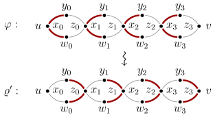
Figure 2. Weight-shifting from vertex $u$ to vertex $v$ using $P$-diamond.

2.10. Regular expander subdigraphs

We call a digraph $D$ is an expander if $\bigl{|}N^{-}(S)\bigr{|}>|S|$ and $\bigr{|}N^{+}(S)\bigr{|}>|S|$ for all nonempty proper $S\subseteq V(D)$.

Suppose that $1/n\ll 1/f,\alpha$. Let $G$ be a digraph of order $n$ with $\delta^{0}(G)\geq(\frac{1}{2}+\alpha)n$. If $F\subseteq G$ and $\Delta^{0}(F)\leq f$, then $G$ contains a spanning $d$-regular subdigraph $H$ such that

1. $H$ contains $F$,

2. $d\leq 25n^{2/3}/\alpha$, and

3. $H$ is an expander.

Proof.

Let $H_{p}$ be the graph we obtain by keeping each edge of $G$ with probability $p\coloneqq n^{-1/3}$, with choices made independently for each edge. With probability $1-\mathrm{o}(1)$

1. every vertex of $H_{p}$ has in- and outdegree at most $4n^{2/3}$, and

2. if $S$ is a nonempty proper subset of $V(G)$, then $\bigl{|}N_{H_{p}}^{-}(S)\bigr{|},\bigl{|}N_{H_{p}}^{+}(S)\bigr{|}>|S|$.

Proof of claim.

Let $x\in H_{p}$. Note that $\deg_{H_{p}}^{-}(x)$ and $\deg_{H_{p}}^{+}(x)$ are binomial random variables with expectation between $(\frac{1}{2}+\alpha)n^{2/3}$ and $n^{2/3}$. By Chernoff (1) (applied with $t=n^{2/3}/2$) we have

(7) $$\begin{split}\mathbb{P}\bigl{(}\deg_{H_{p}}^{-}(x)>4n^{2/3}\bigr{)}&\leq\exp\bigl{(}-n^{2/3}\bigr{)}\quad\text{ and }\\ \mathbb{P}\bigl{(}\deg_{H_{p}}^{+}(x)>4n^{2/3}\bigr{)}&\leq\exp\bigl{(}-n^{2/3}\bigr{)}.\end{split}$$

By a union bound over all $n$ vertices, (a) holds with probability $1-\mathrm{o}(1)$. To prove (b), let $S\subseteq H_{p}$ be proper and nonempty. We will show that $|N_{H_{p}}^{+}(S)|>|S|$; it follows by symmetry that $|N_{H_{p}}^{-}(S)|>|S|$. We consider four cases. If $|S|<n^{1/2}$, then $N^{+}_{H_{p}}(x)$ is a binomial random variable with $\mathbb{E}N^{+}_{H_{p}}(x)\geq(\frac{1}{2}+\alpha)n^{2/3}$ for each $x\in S$. By Chernoff (2) (applied with $t=np/2$) we have, for any $y\in S$, that

(8) $$\mathbb{P}\Bigl{(}|N_{H_{p}}^{+}(S)|\leq|S|\Bigr{)}\leq\mathbb{P}\left(\deg_{H_{p}}^{+}(y)<\frac{np}{2}\right)\leq\exp\Bigl{(}-\frac{n^{2/3}}{8}\Bigr{)}.$$

If $n^{1/2}\leq|S|<n/2$, then $\bigl{|}N_{H_{p}}^{+}(S)\bigr{|}\leq|S|$ if and only if there exists $T\subseteq V(H_{p})$ such that $|T|\geq n-|S|$ and $N_{H_{p}}^{+}(S)\cap T=\varnothing$. Since $|S|<n/2$, we have $n-|S|\geq n/2$; hence for each $T\subseteq V(H_{p})$ with $|T|\geq n-|S|$ and each vertex $x\in S$, we have $\deg_{G}^{+}(x,T)\geq\alpha n$; in particular, $e(H_{p}[S{\color[rgb]{0,0,0}\to}T])$ is a binomial random variable with expectation at least $|S|\alpha n^{2/3}\geq\alpha n^{7/6}$. By Chernoff (2), applied with $t=\alpha n^{7/6}/2$, we have $\mathbb{P}\bigl{(}e(H_{p}[S{\color[rgb]{0,0,0}\to}T])=0\bigr{)}\leq\exp\bigl{(}-\alpha n^{7/6}/8\bigr{)}$. So if $B_{T}$ is the event ‘$e(H_{p}[S{\color[rgb]{0,0,0}\to}T])=0$’ then

(9) $$\mathbb{P}\Bigl{(}\bigl{|}N_{H_{p}}^{+}(S)\bigr{|}\leq|S|\Bigr{)}=\mathbb{P}\Bigl{(}\bigcup_{|T|\geq n-|S|}B_{T}\Bigr{)}\leq 2^{n}\exp\Bigl{(}-\frac{\alpha n^{7/6}}{8}\Bigr{)}\leq\exp\Bigl{(}-\frac{\alpha n^{7/6}}{10}\Bigr{)}.$$

If $n/2\leq|S|<n-n^{1/2}$, then, as before, $\bigl{|}N_{H_{p}}^{+}(S)\bigr{|}\leq|S|$ if and only if there exists $T\subseteq V(H_{p})$ such that $|T|\geq n-|S|\geq n^{1/2}$ and $N_{H_{p}}^{+}(S)\cap T=\varnothing$. Since $|S|\geq n/2$, for all $x\in G$ we have $\deg_{G}^{-}(x,S)\geq\alpha n$. In particular, $e(H_{p}[S{\color[rgb]{0,0,0}\to}T])$ is a binomial random variable with $\mathbb{E}\,e(H_{p}[S{\color[rgb]{0,0,0}\to}T])\geq|T|\alpha n^{2/3}\geq\alpha n^{7/6}$, and thus (9) holds. Finally, if $|S|\geq n-n^{1/2}$, then for all $x\in H_{p}$ we have $\deg_{G}^{-}(x,S)\geq n/2$, and thus $\deg_{H_{p}}^{-}(x,S)$ is a binomial random variable with expectation at least $n^{2/3}/2$. By Chernoff (2)

(10) $$\mathbb{P}\Bigl{(}N_{H_{p}}^{+}(S)\neq V(H_{p})\Bigr{)}\leq\sum_{x\in H_{p}}\mathbb{P}\Bigl{(}\deg_{H_{p}}^{-}(x)\leq n^{1/2}\Bigr{)}\leq\exp\Bigl{(}-\frac{n^{2/3}}{40}\Bigr{)}.$$

For all proper and nonempty $S\subseteq V(H_{p})$, let $P_{S}\coloneqq\mathbb{P}\bigl{(}|N_{H_{p}}^{+}(S)|\leq|S|\bigr{)}$. By a union bound, we obtain

$$\mathbb{P}\bigl{(}\text{\ref{cl:expander} does not hold}\bigr{)}=\sum_{|S|<\sqrt{n}}\,\,P_{S}\quad\,\,+\,\,\quad\sum_{\mathclap{\sqrt{n}\leq|S|<n-\sqrt{n}}}\,\,P_{S}\quad\,\,+\,\,\quad\sum_{\mathclap{n-\sqrt{n}\leq|S|<n}}\,\,P_{S}\\ \leq 3\sqrt{n}\binom{\phantom{\sqrt{n}}\mathllap{n}\,\,}{\sqrt{n}\,\,}\underbracket{\exp\left(-\frac{n^{2/3}}{40}\right)}_{\text{\eqref{e:S-small} and \eqref{e:S-large}}}+2^{n}\underbracket{\exp\left(-\frac{\alpha n^{7/6}}{10}\right)}_{\text{\eqref{e:S-medium}}}=\mathrm{o}(1),$$

where sums range over proper nonempty $S\subseteq H_{p}$ and we use the bounds $\binom{n}{\sqrt{n}}\leq(\sqrt{n}\,e)^{\sqrt{n}}\leq\exp\bigl{(}\sqrt{n}\,\ln n\bigr{)}$. Therefore (b) holds with probability $1-\mathrm{o}(1)$, as desired. ∎

Returning to the proof of the lemma, fix an outcome of $H_{p}$ such that (a) and (b) hold and let $H^{\prime}\coloneqq H_{p}\cup F$. Clearly, if $H^{\prime}\subseteq H\subseteq G$, then $H$ satisfies both (ii) and (iii). Hence, to conclude the proof, if suffices to find such $H$ satisfying (ii). By (a), we have $\Delta^{0}(H^{\prime})\leq 4n^{2/3}+f\leq 5n^{2/3}$ and $e(H^{\prime})\leq 4n^{5/3}+nf\leq 5n^{5/3}$. Hence, by Lemma 2.8, $E(H^{\prime})$ admits a partition $\mathcal{M}$ such that $|\mathcal{M}|\leq 5n^{2/3}+1$ and $|M|-|N|\leq 2$ for all $M,N\in\mathcal{M}$. Fix $d\in\mathbb{N}$ and an equitable partition $M_{1},\ldots,M_{d}$ of $E(H^{\prime})$ (refining $\mathcal{M}$) so that $d\leq 32n^{2/3}/\alpha$ and $|M_{i}|\leq\alpha n/6$ for each $i\in[d]$. The following procedure builds the desired $H$.

Procedure:

Let $G_{0}\coloneqq G-E(H^{\prime})$. For each $i\in[d]$, in order, greedily choose a directed cycle $C_{i}$ in $G_{i-1}\cup M_{i}$, such that $C_{i}$ has length $3|M_{i}|/2$ and covers all edges in $M_{i}$; let $C_{i}^{\prime}$ be a directed Hamilton cycle in $G_{i-1}\smallsetminus V(C_{i})$ and let $G_{i}\coloneqq G_{i-1}\smallsetminus\bigl{(}E(C_{i})\cup E(C_{i}^{\prime})\bigr{)}$. We set $H\coloneqq\bigcup_{i\in[d]}(C_{i}\cup C_{i}^{\prime})$.

Let us check that these steps may be carried out. Fix $i\in[d]$. It suffices to show that $C_{i}$ and $C_{i}^{\prime}$ exist. Let $M_{i}=\{u_{1}{\color[rgb]{0,0,0}\to}v_{1},\ldots,u_{r}{\color[rgb]{0,0,0}\to}v_{r}\}$. Since $\delta^{0}(G_{i})\geq\delta^{0}(G_{0})-d\geq(1/2+3\alpha/4)n$, for each pair of vertices $x,y\in G_{i}$ there exists at least $3\alpha n/4-|M_{i}|$ vertices $z$ such that $z\in(N_{G_{i}}^{+}(x)\cap N_{G_{i}}^{-}(y))\smallsetminus|M_{i}|$. Hence there exist $|M_{i}|/2$ distinct vertices $z_{j}$ with $z_{j}\in(N_{G_{i}}^{+}(v_{j})\cap N_{G_{i}}^{-}(u_{j+1}))\smallsetminus|M_{i}|$ for each $j\in[r]$ (addition modulo $r$). Let $C_{i}$ be the cycle $u_{1}{\color[rgb]{0,0,0}\to}v_{1}{\color[rgb]{0,0,0}\to}z_{1}{\color[rgb]{0,0,0}\to}u_{2}{\color[rgb]{0,0,0}\to}\cdots{\color[rgb]{0,0,0}\to}u_{r}{\color[rgb]{0,0,0}\to}v_{r}{\color[rgb]{0,0,0}\to}z_{r}{\color[rgb]{0,0,0}\to}u_{1}$. Since $|C_{i}|=3|M_{i}|\leq\alpha n/2$, it follows $\delta^{0}\bigl{(}G_{i}\smallsetminus V(C_{i})\bigr{)}\geq(1/2+\alpha/4)n$, so $G_{i}\smallsetminus V(C_{i})$ contains a directed Hamilton cycle $C_{i}^{\prime}$. Finally, note that $H^{\prime}\subseteq H$ and $H$ is the edge-disjoint union of spanning subdigraphs $C_{i}\cup C_{i}^{\prime}$ of $G$, and that for each $i\in[d]$ all vertices in each $C_{i}\cup C_{i}^{\prime}$ has both in- and outdegree $1$. We conclude $H$ is a spanning subgraph of $G$ with $\deg_{H}^{-}(x)=\deg_{H}^{+}(x)=d\leq 32n^{2/3}/\alpha$ for each $x\in H$, so (ii) holds. ∎

2.11. Random walks

Let $D$ be a digraph, let $P$ be an oriented path rooted in one of its leaves, and let $v_{0},v_{1},\ldots,v_{r}$ be an ancestral order of $P$. For each $v\in D$, a random $P$-walk $\mathcal{W}_{P,D}(v)$ on $D$, starting at $v$, is a random walk $X_{0},X_{1},\ldots,X_{r}$ starting at $X_{0}=v$ and such that for each $i\in[r]$ we choose $X_{i}$ as follows: if $v_{i}$ is an outneighbour of $v_{i-1}$ in $P$, then choose $X_{i}$ uniformly at random from $N_{D}^{+}(X_{i-1})$; otherwise choose $X_{i}$ uniformly at random from $N_{D}^{-}(X_{i-1})$, with all choices made independently for all $i$. The following lemmas establish a crucial property of these walks.

Let $D$ be an expander digraph, let $f:V(D)\to[0,1]$ and let $M\coloneqq\max_{x,y\in D}f(x)-f(y)$. If $n\coloneqq|D|\geq 3$ and $M>0$, then there exists $u,x,y\in D$ such that $x,y\in N^{-}(u)$ and $f(y)-f(x)\geq M/(n-1)$ and, similarly there exists $v,w,z\in D$ such that $w,z\in N^{+}(v)$ and $f(w)-f(z)\geq M/(n-1)$.

Proof.

If suffices to prove the existence of $u,x,y$; the statement for $v,w,z$ follows by symmetry. Let $S_{1},\ldots,S_{r}$ be a partition of $V(D)$ such that for all $x,y\in D$ we have $f(x)=f(y)$ if and only if $x,y\in S_{i}$ for some $i\in[r]$. Clearly, $1<r\leq n$. Since $f$ is constant in each set of this partition, we write $f(i)$ for the common value of $f$ over all $x\in S_{i}$. We can assume that the sets are labelled so that $f(i)<f(j)$ whenever $i<j$. Note that $M=f(r)-f(1)$, and therefore $f(j+1)-f(j)\geq M/(r-1)\geq M/(n-1)$ for some $j\in[r-1]$. Let $X\coloneqq S_{1}\cup\cdots\cup S_{j}$ and $Y\coloneqq S_{j+1}\cup\cdots\cup S_{n}$. Since $D$ is an expander, $\bigl{|}N^{+}(X)\bigr{|}>|X|$ and $\bigl{|}N^{+}(Y)\bigr{|}>|Y|$. Because $|X|+|Y|=n$ there must be a vertex $u\in N^{+}(X)\cap N^{+}(Y)$. Let $x\in X$ and $y\in Y$ be inneighbours of $u$. Then $f(y)-f(x)\geq f(j+1)-f(j)\geq M/(n-1)$ as desired. ∎

Let $D$ be an $d$-regular expander digraph of order $k$, and let $P$ be an oriented path of order $n$, rooted in a leaf. For each $v\in V(D)$, if $X_{0},\ldots,X_{n}$ is a random $P$-walk $\mathcal{W}_{P,D}(v)$, then

(11) $$\max_{x\in D}\left(\mathbb{P}(X_{n}=x)-\frac{1}{k}\right)^{\!2}\leq\left(1-\frac{1}{2k^{3}}\right)^{\!n}.$$

Proof.

For each random variable $X$ with finite image $I$, define $m(X)\coloneqq\sum_{x\in I}\left(\mathbb{P}(X=x)-\frac{1}{k}\right)^{\!2}$, so $m(X)=0$ if and only if $\mathbb{P}(X=x)=1/k$ for all $x\in I$. We first prove that

(12) $$m(X)\leq(1-1/k)^{2}+(k-1)/k^{2}=1-k^{-1}<1.$$

Proof of (12).

Note that $1-1/k$ is the value $m(\cdot)$ attains at a random variable which concentrates all ‘weight’ in a single vertex of $D$. Let $X$ be a random variable which maximises $m(X)$ over all random variables with image $D$ and suppose, looking for a contradiction, that there exist distinct $u$ and $v$ in $D$ such that $\mathbb{P}(X=u)>0$ and $\mathbb{P}(X=v)>0$. Define a random variable $Y$ by $Y=X$ if $X\neq u$ and $Y=v$ otherwise. Then $m(Y)=m(X)+2\mathbb{P}(X=u)\mathbb{P}(X=v)>m(X)$, contradicting the choice of $X$. ∎

Returning to the proof of the lemma, let $\mu$ be a probability distribution over $D$, let $v\in D$ be selected according to $\mu$, and let $X_{0},\ldots,X_{n}$ be a random $P$-walk $\mathcal{W}_{P,D}(v)$. We will show that $m(X_{i-1})\geq m(X_{i})$ for all $i\in[n]$, with strict inequality if $m(X_{i-1})>0$. Let $i\in[n]$, suppose that $v_{i-1}$ is an inneighbour of $v_{i}$ in $P$ and define $f(y)\coloneqq\mathbb{P}(X_{i-1}=y)-1/k$ for all $y\in D$. Since $|N_{D}^{-}(x)|=d$ for all $x\in D$, we have

$$m(X_{i})=\sum_{x\in D}\left(\mathbb{P}(X_{i}=x)-\frac{1}{k}\right)^{\!2}=\sum_{x\in D}\Biggl{(}\biggl{(}\sum_{y\in N_{D}^{-}(x)}\frac{\mathbb{P}(X_{i-1}=y)}{d}\biggr{)}-\frac{1}{k}\Biggr{)}^{\!2}\\ =\sum_{x\in D}\biggl{(}\sum_{y\in N_{D}^{-}(x)}\frac{f(y)}{d}\biggr{)}^{\!2}\overset{(\natural)}{\leq}\sum_{x\in D}\,\frac{1}{d}\,\Bigl{(}\!\sum_{y\in N_{D}^{-}(x)}f(y)^{2}\Bigr{)}=\sum_{x\in D}f(x)^{2}=m(X_{i-1})$$

where $(\natural)$ follows by Theorem 2.2 (with $u_{i}=1/d$ and $v_{i}=f(y)$). Moreover, $(\natural)$ is an equality if and only if $f(y)=\alpha/d$ for all $y$ and some $\alpha\neq 0$, i.e., if and only if $X_{i-1}$ is uniformly distributed over $D$. Let $M_{i}\coloneqq\max_{x\in D}\bigl{|}f(y)\bigr{|}$. We have that

$$m(X_{i})=\sum_{x\in D}\biggl{(}\sum_{y\in N_{D}^{-}(x)}\!\!\!\!\frac{f(y)}{d}\biggr{)}^{\!2} \overset{\mathclap{\eqref{e:cauchy-err}}}{=}\,\sum_{x\in D}\left(\sum_{y\in N_{D}^{-}(x)}\!\!\!\!d\left(\frac{f(y)}{d}\right)^{\!\!2}-\!\!\!\!\!\sum_{z,w\in N_{D}^{-}(x)}\!\!\!\!\frac{\bigl{(}f(z)-f(w)\bigr{)}^{2}}{2d^{2}}\right)$$

$$=m(X_{i-1})-\sum_{\mathclap{\begin{subarray}{c}x\in D\\ z,w\in N_{D}^{-}(x)\end{subarray}}}\,\,\frac{\bigl{(}f(z)-f(w)\bigr{)}^{2}}{2d^{2}}\overset{(\sharp)}{\leq}m(X_{i-1})-\frac{M_{i}^{2}}{2d^{2}}$$

where $(\sharp)$ follows from Lemma 2.11. Note that if $m(X_{i-1})=\varepsilon$ then $|f(x)|^{2}\geq\varepsilon/k$ for some $x\in D$, and thus $M_{i}^{2}\geq\varepsilon/k$, so $m(X_{i})\leq m(X_{i-1})-\varepsilon/2kd^{2}<m(X_{i-1})(1-1/2k^{3})$. Therefore,

$$\max_{x\in D}\left(\mathbb{P}(X_{n}=x)-\frac{1}{k}\right)^{\!2}\leq m(X_{n})\leq m(X_{0})\left(1-\frac{1}{2k^{3}}\right)^{\!n}\,\,\overset{\mathclap{\eqref{e:m(.)}}}{<}\,\left(1-\frac{1}{2k^{3}}\right)^{\!n}.\qed$$

3. Allocation, embedding, and an approximate result

In this section we discuss the allocation and embedding algorithms (Lemmas 3.1, 3.2 and Theorem 1).

Lemma 3.1 states that the allocation algorithm (Algorithm 1) distributes vertices somewhat evenly among clusters in the reduced graph (if the latter is a regular expander). Lemma 3.2 states that if $G$ is a digraph with an appropriate reduced graph $R$, and if we are given an appropriate allocation (such as the one guaranteed by Lemma 3.1) of a tree $T$ to $R$, then the embedding algorithm successfully finds a copy of $T$ in $G$. Finally, Theorem 1 combines these lemmas, showing that if $T$ is a tree with maximum degree $|T|^{\mathrm{o}(1)}$, and if $G$ is a digraph with large minimum semidegree and order slightly greater than $|T|$, then $G$ contains a copy of $T$.

3.1. Allocation algorithm

Let $F,R$ be digraphs. An allocation of $F$ to $R$ is a homomorphism from $F$ to $R$. In our applications, $R$ will usually be a suitable reduced digraph of the host graph $G$.

Algorithm 1 below is a randomised procedure which defines an allocation of a rooted tree $T$ to a digraph $D$, and is inspired by a similar procedure in [15, Section 3.2]. The algorithm in [15], however, is only applied when $D$ is a directed cycle with loops in every vertex (i.e., $v{\color[rgb]{0,0,0}\to}v\in E(D)$ for all $v\in D$), whereas here there are no loops but we require that $\delta^{0}(D)\geq 1$. Essentially, Algorithm 1 steps through the vertices of $T$ in an ancestral order, and defines the homomorphism $\varphi:T\to D$ uniformly at random at each step, with the restriction that siblings (i.e., vertices with the same parent) are mapped to the same vertex if the edge between them and the parent has the same orientation.

Input : an oriented tree $T$ of order $n$, with root $t_{1}$, an ancestral order $t_{1},\ldots,t_{n}$ of $T$, a digraph $D$ with $\delta^{0}(D)\geq 1$ and $x_{1}\in V(D)$.

for $\tau=1$ to $n$ do

      if $\tau=1$ then define $\varphi(t_{1})\coloneqq x_{1}$.

       else if $\varphi(t_{\tau})$ is undefined then

            Let $t_{\sigma}$ be the parent of $t_{\tau}$ and let $x_{\sigma}=\varphi(t_{\sigma})$.

             Pick $x_{\tau}^{+}\in N_{D}^{+}(x_{\sigma})$ and $x_{\tau}^{-}\in N_{D}^{-}(x_{\sigma})$ uniformly at random independently of all other choices.

             Let $t_{\tau}^{1},\ldots,t_{\tau}^{s}$ be the children of $t_{\sigma}$.

             for $i=1$ to $s$ do

                   if $t_{\tau}^{i}\in N_{T}^{+}(t_{\sigma})$ then define $\varphi(t_{\tau}^{i})\coloneqq x_{\tau}^{+}$.

                   else define $\varphi(t_{\tau}^{i})\coloneqq x_{\tau}^{-}$.

                  

            

      

Algorithm 1 The Vertex Allocation Algorithm

We next show that Algorithm 1 always builds a homomorphism and, moreover, that if $T$ is sufficiently large and $D$ is a regular expander, then it distributes vertices of $T$ roughly evenly among vertices of $D$.

Let $T$ be an oriented tree of order $n$ rooted at $r$, let $D$ be a regular expander digraph of order $k$, and let $x\in D$. If $\varphi$ is the allocation we obtain by applying the allocation algorithm (Algorithm 1) to $T$ and $D$, then the following properties hold.

1. $\varphi$ is a homomorphism $\varphi:T\to D$ and $\Delta(\varphi)\leq 3$; moreover, $|\varphi^{-1}(N_{T}^{-}(r))|+|\varphi^{-1}(N_{T}^{+}(r))|\leq 2$.

2. Let $u,v\in V(T)$, where $u$ lies on the path from $r$ to $v$, let $P$ be the path between $u$ and $v$, and let $W\coloneqq V(P)\smallsetminus\{u\}$. For all $j\in D$, the allocation of $W$, conditioned on the event ‘$\varphi(u)=j$’ is a random $P$-walk on $D$.

3. Suppose that $1/m\ll 1/k$. Let $u,v\in V(T)$ be such that $u$ lies on the path from $r$ to $v$, and $\operatorname{dist}_{T}(u,v)\geq{4k^{3}\log m}$. Then for all $i,j\in D$,

   $$\mathbb{P}(\,\text{$v$ is allocated to\leavevmode\nobreak\ $i$}\mid\text{$u$ is allocated to\leavevmode\nobreak\ $j$}\,)=\frac{1}{k}\left(1\pm\frac{1}{m}\right).$$

4. Suppose that $1/n\ll 1/K\ll 1/k,\zeta$ and $\Delta(T)\leq n^{(K\log n)^{-1/2}}$. If $S\subseteq V(T)$ and $|S|\geq n^{2/3+\zeta}$, then with probability $1-\mathrm{o}(1)$ each of the vertices of $D$ has $|S|\bigl{(}\frac{1}{k}\pm n^{-(\log n)^{-1/2}}\bigr{)}$ vertices of $S$ allocated to it.

5. Suppose that $1/n\ll 1/K\ll 1/k,\beta$, that $\Delta(T)\leq n^{(K\log n)^{-1/2}}$, and that $D$ is $d$-regular. For all $Q\subseteq E(D)$, if $S\subseteq E(T)$ contains at least $\beta n$ vertex-disjoint edges, then $\varphi$ allocates at least $|S|/4kd$ edges of $S$ to each edge of $Q$ with probability $1-\mathrm{o}(1)$.

Similar statements to (c) and (d) were included in [18, Lemma 3.2], with a similar proof.

Proof.

Note that every edge of $T$ is mapped to an edge of $D$; moreover, for all $v\in T$, the neighbours of $v$ fall in $3$ categories: parent, in- or outchild of $v$, and all vertices in each of these categories are allocated to the same cluster, so (a) holds (the moreover part holds since $r$ has no parent). In particular, (b) also holds, since the allocation of vertices along any path match the choices that would be made in a random $P$-walk. From this point onward, let us assume $V(D)=[k]$. We now prove item (c). Let $P(u,v)\subseteq T$ be the (oriented) path $u=v_{0}v_{1}\cdots v_{\ell}=v$ from $u$ to $v$, so $\ell\geq 4k^{3}\log m$. Suppose that $u$ has been allocated to $x_{0}\in D$, and for all $i\in\{0,1,\ldots,\ell\}$ let $X_{i}$ be the vertex to which $v_{i}$ is allocated (so $X_{0}=x_{0}$), so $X_{0},X_{1},\ldots,X_{\ell}$ is a random $P$-walk by (c). This implies (c), since, by Lemma 2.11, for all $x\in D$ we have

$$\mathbb{P}(X_{n}=x)=\frac{1}{k}\pm\left(1-\frac{1}{2k^{3}}\right)^{\ell/2}=\frac{1}{k}\pm\mathrm{e}^{-\ell/4k^{3}}=\frac{1}{k}\left(1\pm\frac{1}{m}\right).$$

We now turn to (d). By Lemma 2.1, there exists an integer $s\leq 3n^{1/3}$, vertices $v_{1},\ldots,v_{s}\in V(T)$ and pairwise-disjoint subsets $F_{1},\ldots,F_{s}$ of $V(T)$ such that for all $i,j\in[s]$ we have $|\bigcup_{i=1}^{s}F_{i}|\geq n-n^{5/12}$, $|F_{i}|\leq n^{2/3}$, and if $j<i$ then any path from $r$ or any vertex of $F_{j}$ to any vertex of $F_{i}$ passes through the vertex $v_{i}$, where $\operatorname{dist}(v_{i},F_{i})\geq{K\log\Delta(T)/13}$. Let $\delta_{n}\coloneqq 4k/\bigl{(}n^{(K\log n)^{-1/2}}\bigr{)}^{K/52k}<n^{-(\log n)^{-1/2}}$; we shall prove that

$$(\dagger)\quad\parbox{355.57156pt}{with probability\leavevmode\nobreak\ $1-\mathrm{o}(1)$, for all\leavevmode\nobreak\ $j\in[k]$ at most $|S|(\frac{1}{k}+\frac{\delta_{n}}{2k})$ vertices from\leavevmode\nobreak\ $\bigcup_{i\in[s]}F_{i}\cap S$ are allocated to cluster\leavevmode\nobreak\ $V_{j}$.}$$

Note that ($\dagger$) implies (d). Indeed, the number of vertices of $T$ not contained in any of the sets $F_{i}$ is at most $n^{5/12}\leq\delta_{n}|S|/2k$; if ($\dagger$) holds, then with probability $1-\mathrm{o}(1)$ at most $|S|(1+\delta_{n})/k$ vertices of $S$ are allocated to each $V_{j}$. Hence, at least $|S|-(k-1)|S|(1+\delta_{n})/k\geq|S|(1/k-\delta_{n})$ vertices of $S$ are allocated to each $V_{j}$, so (d) holds (since $\delta_{n}<n^{-(\log n)^{-1/2}}$). To prove ($\dagger$), define random variables $X_{i}^{j}$ for each $i\in[s]$ and $j\in[k]$ by

$$X_{i}^{j}\coloneqq\frac{\text{\# of vertices of\leavevmode\nobreak\ $F_{i}\cap S$ allocated to cluster\leavevmode\nobreak\ $V_{j}$}}{n^{2/3}},$$

so each $X_{i}^{j}$ lies in the range $[0,1]$. Note that the cluster to which a vertex $x$ of $T$ is allocated is dependent only on the cluster to which the parent of $x$ is allocated and on the outcome of the random choice made when allocating $x$. For each $q\in[k]$, we have $\mathbb{E}(\,X_{i}^{j}\mid X_{i-1}^{j},\ldots,X_{1}^{j},v_{i}\in V_{q}\,)=\mathbb{E}(\,X_{i}^{j}\mid v_{i}\in V_{q}\,)$, where we write $x\in V_{q}$ to denote the event that $x$ is allocated to $V_{q}$. So for any $i\in[s]$ and ${j\in[k]}$ we have

$$\mathbb{E}(\,X_{i}^{j}\mid X_{i-1}^{j},\ldots,X_{1}^{j}\,)\leq\max_{q\in[k]}\mathbb{E}(\,X_{i}^{j}\mid X_{i-1}^{j},\ldots,X_{1}^{j},v_{i}\in V_{q}\,)\\ =\max_{q\in[k]}\mathbb{E}(\,X_{i}^{j}\mid v_{i}\in V_{q}\,)=\max_{q\in[k]}\frac{\sum_{x\in F_{i}\cap S}\mathbb{P}(\,x\in V_{j}\mid v_{i}\in V_{q}\,)}{n^{2/3}}\overset{\ref{l:alloc-prop-iii}}{\leq}\left(\frac{1}{k}+\frac{\delta_{n}}{4k}\right)\frac{|F_{i}\cap S|}{n^{2/3}}.$$

We apply Lemma 2.2 with

$$\mu\coloneqq\left(\frac{1}{k}+\frac{\delta_{n}}{4k}\right)\frac{|S|}{n^{2/3}} \geq\left(\frac{1}{k}+\frac{\delta_{n}}{4k}\right)\sum_{i\in[s]}\frac{|F_{i}\cap S|}{n^{2/3}},$$

which (since $$1/n\ll 1/k,\zeta$$) yields

$$\mathbb{P}\Bigl{(}\sum_{i\in[s]}X_{i}^{j}>(1+\delta_{n}/8)\mu\Bigr{)} \leq\exp\left(\frac{-(\delta_{n}/8)^{2}\mu}{3}\right)=\exp\left(-\frac{\delta_{n}^{2}(1+\delta_{n}/4)|S|}{192kn^{2/3}}\right)\leq\exp\bigl{(}-n^{\zeta/2}\bigr{)}.$$

By a union bound, with probability $1-\mathrm{o}(1)$, we have

$$n^{2/3}\sum_{i\in[s]}X_{i}^{j}\leq n^{2/3}(1+\delta_{n}/8)\mu\leq|S|\left(\frac{1}{k}+\frac{\delta_{n}}{2k}\right)\qquad\text{for all\leavevmode\nobreak\ {$j\in[k]$}.}$$

That is, for each $j\in[k]$, at most $|S|\bigl{(}\frac{1}{k}+\frac{\delta_{n}}{2k}\bigr{)}$ vertices in $\bigcup_{i=1}^{r}F_{i}\cap S$ are allocated to $V_{j}$, so ($\dagger$) holds.

To conclude, let $\prec$ be an ancestral order of $T$ and, for each edge $e\in S$, let $x_{e}$ and $y_{e}$ be the endvertices of $e$, labelled so that $x_{e}\prec y_{e}$. At least half of the edges in $S$ have the same orientation with respect to $\prec$, so let $S^{\prime}$ be a subset of $S$ with at least $|S|/2$ such edges which are all oriented, say, from $x_{e}$ to $y_{e}$. Let $u_{1}{\color[rgb]{0,0,0}\to}v_{1},\ldots,u_{q}{\color[rgb]{0,0,0}\to}v_{q}$ be the edges in $Q$. By item (d), with probability $1-\mathrm{o}(1)$ there are at least $|S^{\prime}|\bigl{(}\frac{1}{k}\pm n^{-(\log n)^{-1/2}}\bigr{)}$ vertices $x_{e}\in e\in S^{\prime}$ allocated to each $u_{j}$ for all $j\in[q]$. Call this event $E_{1}$. Conditioned on the $E_{1}$, and for each $j\in[q]$, let $Z_{j}$ be the number of edges of $S^{\prime}$ which are allocated to $u_{j}{\color[rgb]{0,0,0}\to}v_{j}$; then, for any fixed $j\in[q]$, since $D$ is $d$-regular (and $d\leq\binom{k}{2}$), it follows that $Z_{j}$ is a binomial random variable with expectation at least $|S^{\prime}|/d$, so the probability that $Z_{j}<|S^{\prime}|/2d$ decreases exponentially with $n$. By a union bound (over these $q$ events), it follows that with probability $1-\mathrm{o}(1)$ we have that $Z_{j}\geq|S^{\prime}|/2d\geq|S|/4kd$ for all $j\in[q]$; we call this event $E_{2}$. Since both $E_{1}$ and $E_{2}|E_{1}$ (i.e., $E_{2}$ conditioned on the occurrence of $E_{1}$) happen with probability $1-\mathrm{o}(1)$, we conclude (e) holds as required. ∎

3.2. Embedding algorithm

In this section we describe the tree-embedding algorithm we use (with a few modifications) to prove Lemmas 5.2 and 4.2 and Theorem 1. It embeds a rooted tree $T$ to a digraph $G$ with reduced graph $R$, respecting a given homomorphism $\varphi:T\to R$. Vertices are embedded greedily so that each vertex $x\in T$ is embedded to the cluster corresponding to $\varphi(x)$. The main result of this section (Lemma 3.2) states sufficient conditions that guarantee the algorithm succeeds. For each $v\in T$, let $C^{-}(v)$ be the children of $v$ in $N^{-}_{T}(v)$, $C^{+}(v)$ be the children of $v$ in $N^{+}_{T}(v)$ and $\text{{{\color[rgb]{0.6,0,0}\emph{$C(v)$}}}}\coloneqq C^{-}(v)\cup C^{+}(v)$. We write $S(x)$ to denote the star $T\bigl{[}\{x\}\cup C(x)\bigr{]}$ induced by $x$ and its children.

$\blacktriangleright$Embedding algorithm. If at any point in the description below there is more than one possible choice available, we take the lexicographically first of these, so that for each input the output is uniquely defined and — thus making the algorithm deterministic. Furthermore, if at any point some required choice cannot be made, terminate with failure. At each time $\tau$, with $1\leq\tau\leq n$, we shall embed a vertex $t_{\tau}$ to a vertex $v_{\tau}\in V_{\varphi(t_{\tau})}$; we will also reserve sets $A_{\tau}^{-},A_{\tau}^{+}$ for the children of $t_{\tau}$. We say that a vertex $t_{s}$ of $T$ is open at time $\tau$ if $t_{s}$ has been embedded but some child of $t_{s}$ has not yet been embedded.

$\blacktriangleright$Input. An oriented tree $T$ with ancestral order $t_{1}\prec\ldots\prec t_{n}$, a digraph $R$, a homomorphism $\varphi:T\to R$, a digraph $G$, a partition $\mathcal{V}\coloneqq\{\,V_{i}:i\in R\,\}$ of $V(G)$, a vertex $v_{1}\in V_{\varphi(t_{1})}$ and constants $\beta$ and $\gamma$.

$\blacktriangleright$Procedure. At each time $\tau$, with $1\leq\tau\leq n$, we take the following steps.

$\blacktriangleright$Step 1. Define the set $B^{\tau}$ of vertices of $G$ unavailable for use at time $\tau$ to consist of the vertices already occupied and the sets reserved for the children of open vertices, so

$$B^{\tau}\coloneqq\{v_{1},\dots,v_{\tau-1}\}\cup\bigcup_{t_{s}\colon t_{s}\textrm{ is open}}\bigl{(}A_{s}^{-}\cup A_{s}^{+}\bigr{)}$$

For each $V_{i}\in\mathcal{V}$, let $V_{i}^{\tau}\coloneqq V_{i}\smallsetminus B^{\tau}$, so $V_{i}^{\tau}$ is the set of available vertices of $V_{i}$.

$\blacktriangleright$Step 2. If $\tau=1$ embed $t_{1}$ to $v_{1}$. Alternatively, if $\tau>1$:

1. Let $t_{\sigma}$ be the parent of $t_{\tau}$ (so $A_{\sigma}^{-},A_{\sigma}^{+}$ were reserved for the children of $t_{\sigma}$).

2. If $t_{\sigma}{\color[rgb]{0,0,0}\to}t_{\tau}$, let $W\coloneqq A_{\sigma}^{+}\cap V_{\varphi(t_{\tau})}$; otherwise let $W\coloneqq A_{\sigma}^{-}\cap V_{\varphi(t_{\tau})}$.

3. Choose $v_{\tau}\in W$ such that

   (13) $$\begin{split}\deg_{G}^{-}(v_{\tau},V_{i}^{\tau})&\geq\gamma m\qquad\text{for all }i\in\varphi\bigl{(}C^{-}(t_{\tau})\bigr{)},\\ \deg_{G}^{+}(v_{\tau},V_{j}^{\tau})&\geq\gamma m\qquad\text{for all }j\in\varphi\bigl{(}C^{+}(t_{\tau})\bigr{)}.\end{split}$$

4. Embed $t_{\tau}$ to $v_{\tau}$.

$\blacktriangleright$Step 3. In Step 2 we embedded $t_{\tau}$ to a vertex $v_{\tau}\in W$. For each $t_{\pi}\in C^{-}(t_{\tau})$, choose $A_{\pi}^{-}\subseteq N_{G}^{-}(v_{\tau})\cap V_{\varphi(t_{\pi})}^{\tau}$ containing at most $2m^{1-1/\Delta(\varphi)}$ vertices and which is $(\beta{},\gamma,\varphi,m)$-good for $S(t_{\pi})$; let $A_{\tau}^{-}$ be the union of these sets. Similarly, for each $t_{\mu}\in C^{+}(\tau)$, choose a set $A_{\mu}^{+}\subseteq N_{G}^{+}(v_{\tau})\cap V_{\varphi(t_{\mu})}^{\tau}$ containing at most $2m^{1-1/\Delta(\varphi)}$ vertices and which is $(\beta{},\gamma,\varphi,m)$-good for $S_{\mu}$; choose these sets so that they are pairwise disjoint and let $A_{\tau}^{+}$ be their union.

$\blacktriangleright$Termination. Terminate after processing each of $T$, yielding the embedding $\psi(t_{i})=v_{i}$ for each $t_{i}\in T$.

Suppose $1/n\ll 1/K\ll 1/k\ll\varepsilon\ll\gamma\ll\beta\ll d\ll\alpha\leq 2$ and let $m\coloneqq n/k$.

1. Let $T$ be an oriented tree with $|T|\leq n$, $\Delta(T)\leq n^{(K\log n)^{-1/2}}$, root $t_{1}$ and tidy ancestral order $\prec$.

2. Let $R$ and $G$ be digraphs, with $|R|=k$, and suppose there exists a partition $\{\,V_{i}:i\in R\,\}$ of $V(G)$ such that $(1+\alpha)m\leq|V_{i}|\leq 3m$ for each $i\in R$.

3. Let $\varphi$ be a homomorphism from $T$ to $R$ such that $\Delta(\varphi)\leq 4$, each edge $x{\color[rgb]{0,0,0}\to}y\in E(T)$ is mapped to an $(d,\varepsilon)$-regular pair $G[V_{\varphi(x)}{\color[rgb]{0,0,0}\to}V_{\varphi(y)}]$, and which maps at most $(1+\alpha/2)m$ vertices to each $V_{i}$.

4. Let $v_{1}\in V_{\varphi(t_{1})}$ be such that $\deg_{G}^{-}(v_{1},V_{\varphi(x)}),\deg_{G}^{+}(v_{1},V_{\varphi(y)})\geq\gamma m$ for all $x\in C^{-}(t_{1})$, $y\in C^{+}(t_{1})$.

Assuming the above, the embedding algorithm (with parameters $\beta,\gamma$) successfully embeds $T$ to $G$.

Remark. Any fixed constant $q$ with $\alpha\ll 1/q$ could replace $4$ in the bound $\Delta(\varphi)\leq 4$ in (iii) above.

Proof.

The Vertex Embedding Algorithm will only fail if at some point it is not possible to make a required choice. We will show this is never the case, hence the algorithm succeeds.

Since we embed each $x\in T$ to $V_{\varphi(x)}$, at each time $\tau$ we have $\{v_{1}\ldots,v_{\tau-1}\}\cap V_{j}\leq(1+\alpha/2)m$ for each $j\in[k]$. Moreover, if $t_{\sigma}\in T$ is open at the time $\tau$, then $\sigma<\tau$ and $t_{\sigma}$ has a child $t_{\rho}$ with $\tau\leq\rho$. Since we are processing the vertices of $T$ in a tidy order, there can be at most $\Delta(T)\log_{2}n$ of these children vertices $t_{\rho}\in T$; since each reserved set has size $2m^{1-1/\Delta(\varphi)}$, at time $\tau$, the number of reserved vertices (for children of open vertices) is at most $(2m^{1-1/\Delta_{\varphi}})\Delta(T)(\log_{2}n)\leq\alpha m/4$. Hence $|B^{\tau}\cap V_{j}|\leq(1+\alpha/2)m+\alpha m/4$ for each $j$, and $|V_{j}^{\tau}|\geq\alpha m/4$.

Let us check that all required choices can be made. Indeed, in Step (2.3) we choose $v_{\tau}\in W$ satisfying (13). But $W$ is $(\beta{},\gamma,\varphi,m)$-good for $S_{t_{\tau}}$ — it has been reserved at Step 3 when processing vertex $t_{\sigma}$. In particular, $W$ contains at least $\gamma m^{1/\Delta(\varphi)}$ vertices $z$ such that $\deg_{G}^{-}(z,V_{\varphi(x)}^{\tau})\geq\gamma m$ and $\deg_{G}^{+}(z,V_{\varphi(y)}^{\tau})\geq\gamma m$ for all $x\in C^{-}(t_{\tau})$ and all $y\in C^{+}(t_{\tau})$. Moreover, $t_{\sigma}$ has been open since time $\sigma<\tau$ and hence the only vertices which have been embedded to $W$ are children of $t_{\sigma}$ (of which there are at most $\Delta(T)<\gamma m^{1/\Delta(\varphi)}/2$), so we can choose $v_{\tau}$ as required.

Finally, in Step 3 we wish to choose $A_{x}^{-}\subseteq N_{G}^{-}(v_{\tau})\cap V_{\varphi(x)}^{\tau}$ and $A_{y}^{+}\subseteq N_{G}^{+}(v_{\tau})\cap V_{\varphi(y)}^{\tau}$ for each $x\in C^{-}(t_{\tau})$ and each $y\in C^{+}(t_{\tau})$, such that $A_{x}^{-}$ is $(\beta,\gamma,\varphi,m)$-good for $S_{x}$ and $A_{y}^{+}$ is $(\beta,\gamma,\varphi,m)$-good for $S_{y}$. By (13), $v_{\tau}$ has at least $\gamma m$ inneighbours in $V_{\varphi(x)}^{\tau}$ for each $x\in C^{-}(t_{\tau})$ and at least $\gamma m$ outneighbours in $V_{\varphi(y)}^{\tau}$ for each $y\in C^{+}(t_{\tau})$; for $\tau=1$ this holds by our hypothesis (iv) instead. Since $\bigl{|}C^{-}(t_{\tau})\bigr{|}+\bigl{|}C^{+}(t_{\tau})\bigr{|}\leq\Delta(T)$, the total number of vertices which will be reserved in Step 3 is at most $\Delta(T)2m^{1-1/\Delta(\varphi)}\leq\gamma m/3$. Therefore, for each $x\in C^{-}(t_{\tau})$ we have that at any point during Step 3, $V_{\varphi(x)}^{\tau}\cap N_{G}^{-}(v_{\tau})$ contains at least $\gamma m-\gamma m/3>\gamma m/2$ unreserved vertices. Similarly, for each $y\in C^{+}(t_{\tau})$ we have that at any point during Step 3, $V_{\varphi(y)}^{\tau}\cap N_{G}^{-}(v_{\tau})$ contains at least $\gamma m-\gamma m/3>\gamma m/2$ unreserved vertices. Hence, by Lemma 2.7, it follows that for all $x\in C^{-}(t_{\tau})$ and all $y\in C^{+}(t_{\tau})$ there exist $(\beta,\gamma,\varphi,m)$-good sets for $S_{x}$ and $S_{y}$, each of size at most $2m^{1/\Delta(\varphi)}$ and containing only unreserved vertices of $V_{\varphi(x)}^{\tau}$ and $V_{\varphi(y)}^{\tau}$, respectively. Hence the choices in Step 3 can be made as well. ∎

3.3. Proof of Theorem 1

We combine Lemmas 3.1 and 3.2 to embed almost-spanning trees.

Proof of Theorem 1.

Let $G$ be a digraph of order $(1+\varepsilon)n$ such that $\delta^{0}(G)\geq(1/2+\alpha)n$. We introduce constants $\varepsilon^{\prime},d,k,\eta$ such that $\frac{1}{n}\ll\frac{1}{K}\ll\frac{1}{k}\ll\varepsilon^{\prime}\ll d\ll\eta\ll\alpha,\varepsilon$, and apply Lemma 2.7 to obtain a partition $V_{0}\mathbin{\dot{\cup}}V_{1}\mathbin{\dot{\cup}}\cdots\mathbin{\dot{\cup}}V_{k}$ and a digraph $R^{\star}$ with $V({R^{\star}})=[k]$ such that

1. $|V_{0}|<\varepsilon^{\prime}n$ and $m\coloneqq|V_{1}|=\cdots=|V_{k}|$;

2. For each $i\in[k]$ we have $G[V_{i-1}{\color[rgb]{0,0,0}\to}V_{i}]$ and $G[V_{i}{\color[rgb]{0,0,0}\to}V_{i+1}]$ are $(d,\varepsilon^{\prime})$-super-regular;

3. For all $i,j\in[k]$ we have $i{\color[rgb]{0,0,0}\to}j\in E({R^{\star}})$ precisely when $G[V_{i}{\color[rgb]{0,0,0}\to}V_{j}]$ is $(d,\varepsilon^{\prime})$-regular.

4. For all $i\in[k]$ we have $\deg_{R^{\star}}^{0}(i,[k])\geq(1/2+\eta)k$.

Introduce constants $\beta,\gamma$ such that $1/n\ll 1/K\ll 1/k\ll\varepsilon^{\prime}\ll\gamma\ll\beta,d\ll\eta$. Note that $m\geq(1+\varepsilon/2)n/k$ and that $R^{\star}$ contains a regular expander $D$ by Lemma 2.10. Let $T$ be as in the statement of the lemma, fix $r\in T$ and a vertex $x\in D$. Since $T,r,D$ and $x$ satisfy the hypotheses of Lemma 3.1, Algorithm 1 yields a homomorphism $\varphi:T\to D$ such that $\Delta(\varphi)\leq 3$ and $\bigl{|}\varphi^{-1}(V_{i})\bigr{|}=n/k\pm n/n^{-(\log n)^{-1/2}}\leq(1+\varepsilon/4)n/k$ for all $i\in[k]$. By Lemma 2.7, there exists $v_{1}\in V_{\varphi(r)}$ such that for each $x\in C^{-}(r)$, $y\in C^{+}(r)$ we have $\deg_{G}^{-}(x,V_{\varphi(x)})\geq\gamma m$ and $\deg_{G}^{+}(y,V_{\varphi(x)})\geq\gamma m$. Note $T,x,G,v_{1},D,\varphi$ and the constants above (with $\varepsilon/4$ as $\alpha$) satisfy the hypotheses of Lemma 3.2, so the embedding algorithm (applied with these parameters) successfully embeds $T$ to $G$. ∎

4. Spanning trees with many bare paths

The main result of this section is Lemma 4.2 (Theorem 1 for spanning trees with many bare paths). We rely on the Allocation Algorithm (Algorithm 1) and the Embedding Algorithm (Section 3.2), but these procedures must be adapted, because the trees are spanning. Lemma 4.1 below guarantees the existence of a special allocation of vertices; the changes in the embedding are described in the proof of Lemma 4.2.

4.1. Allocation

We first establish the existence of a useful allocation of the tree.

Suppose $\frac{1}{n}\ll\frac{1}{K}\ll\frac{1}{k}\ll\varepsilon\ll\lambda\ll\eta\ll\alpha$. Let $T$ be an oriented tree of order $n$ such that $\Delta(T)\leq n^{-(K\log n)^{-1/2}}$. Suppose that there exists a collection $\mathcal{P}$ of $\lambda n$ vertex-disjoint bare paths of $T$ with order 7. Let ${R^{\star}}$ be a graph with vertex set $V_{0}\mathbin{\dot{\cup}}[k]$, such that $|V_{0}|<\varepsilon n$, where $n-|V_{0}|\equiv 0\bmod k$, and such that for each $i\in[k]$ we have $\deg_{R^{\star}}^{0}(i,[k])\geq(1/2+\eta)k$ and for each $v\in V_{0}$ we have $\deg_{R^{\star}}^{0}(v,[k])>\alpha k$. Suppose also that $H$ is a directed Hamilton cycle in ${R^{\star}}\bigl{[}[k]\bigr{]}$. Then there exists a tidy ancestral order $\prec$ of $T$, disjoint $\mathcal{P}^{0},\mathcal{P}^{H}\subseteq\mathcal{P}$ and a homomorphism $\varphi:T\to{R^{\star}}$ such that

1. $\Delta(\varphi)\leq 4$;

2. $|\mathcal{P}^{0}|=|V_{0}|$ and for each $P\in\mathcal{P}^{0}$ the centre of $P$ is mapped to $V_{0}$;

3. $\varphi$ maps precisely one vertex of $T$ to each $v\in V_{0}$;

4. $\varphi$ maps at least $\lambda n/48k$ centres of paths in $\mathcal{P}^{H}$ to each $i\in[k]$;

5. If $N\coloneqq\{\,N_{T}^{-}(x)\cup N_{T}^{+}(x):\varphi(x)\in V_{0}\,\}$, then $|\varphi^{-1}(i)\cap N|\leq 2\varepsilon n/\alpha k$ for each $i\in[k]$;

6. For each $P\in\mathcal{P}^{H}$, the restriction of $\varphi$ to $\operatorname{middle}(P)$ is a homomorphism from $\operatorname{middle}(P)$ to $H$;

7. $\bigl{|}\varphi^{-1}(1)\bigr{|}=\bigl{|}\varphi^{-1}(2)\bigr{|}=\cdots=\bigl{|}\varphi^{-1}(k)\bigr{|}$.

The proof is divided in four stages, which we now outline. In the setup we fix a tree partition $\{T_{1},T_{2}\}$ of $T$ and a tidy ancestral order $\prec$, such that $T_{1}$ contains a collection $\mathcal{P}^{\prime}$ of many bare paths whose middles are $\prec$-isomorphic to some rooted path $P_{\mathrm{ref}}$. We also fix a partition $\mathcal{P}^{\prime}=\mathcal{P}^{0}\mathbin{\dot{\cup}}\mathcal{P}^{H}\mathbin{\dot{\cup}}\mathcal{P}^{\diamond}$ such that $|\mathcal{P}^{0}|=|V_{0}|$ and $|\mathcal{P}^{H}|,|\mathcal{P}^{\diamond}|\geq|\mathcal{P}^{\prime}|/4$, and map $\operatorname{middle}(P)$ for each path in $\mathcal{P}^{\prime}$ in the following manner. For each $P\in\mathcal{P}^{0}$, we map $\operatorname{middle}(P)$ so that each $c(P)$ is mapped (bijectively) to a vertex in $V_{0}$ and the neighbours of such vertices are mapped to vertices in $[k]$ somewhat evenly. For each $P\in\mathcal{P}^{H}$, we map $\operatorname{middle}(P)$ along $H$ so that the same number of centres are mapped to each $i\in[k]$. Next, we find a spanning subgraph $J^{\diamond}$ of ${R^{\star}}\bigl{[}[k]\bigr{]}$ which is $P_{\mathrm{ref}}$-connected, and map $\operatorname{middle}(P)$ for all $P\in\mathcal{P}^{\diamond}$ so that for each diamond $\textstyle x{\leavevmode\hbox{\set@color \leavevmode\hbox to6.2pt{\vbox to7.49pt{\text{[drawing]}}}}}\genfrac{.}{.}{0.0pt}{}{y}{w}{\leavevmode\hbox{\set@color\reflectbox{\leavevmode\hbox{\set@color \leavevmode\hbox to6.2pt{\vbox to7.49pt{\text{[drawing]}}}}}}}z\subseteq J^{\diamond}$ a linear number of (middles of) paths is mapped to $xyz$ and a linear number of (middles of) paths is mapped to $xwz$ — this will be useful in the last stage of the proof. Finally, we let $T_{1}^{\prime}$ be the tree we obtain from $T_{1}$ by contracting all edges in each path $P\in\mathcal{P}^{\prime}$.

In phase 1 we apply Lemma 2.10 to find a regular expander $J\subseteq{R^{\star}}$ and then allocate $T_{1}^{\prime}$ to $J$ using Algorithm 1. We concatenate this allocation to the maps defined in the setup and complete (greedily) the allocation of the contracted paths, obtaining a homomorphism of $T_{1}$ into $R^{\star}$. By Lemmas 2.8 and 3.1, this allocation of $T_{1}$ is almost uniform over $[k]$, with error $\operatorname{O}(\lambda n/\eta k)$.

In phase 2 we apply Algorithm 1 again, this time allocating $T_{2}$ to a regular expander $J^{\mathrm{blow}}$ which is a subgraph of a weighted blow-up of ${R^{\star}}\bigl{[}[k]\bigr{]}$. The allocation we obtain is again almost uniform, but biased so as to correct the linear errors introduced in the setup stage when embedding paths in $\mathcal{P}^{\prime}$. Altogether, the maps we defined form an allocation of $T$ to $R^{\star}$. We argue that the resulting allocation of $T$ satisfies all of the properties stated in the lemma, except perhaps (vii). However, by Lemma 3.1, we have at most sublinear errors in the order of the preimages of each $i\in[k]$.

To conclude the proof, in phase 3 we modify the mapping of the centres of paths in $\mathcal{P}^{\diamond}$ along $J^{\diamond}$, so as to ensure (vii). This requires only a sublinear number of changes, and thus is possible by Lemma 2.9.

Proof.

As outlined above, this proof is divided in four parts.

$\blacktriangleright$Setup. By Lemma 2.1, $T$ admits a tree-partition $\{T_{1},T_{2}\}$ such that each $T_{i}$ contains at least $\lambda n/3$ paths of $\mathcal{P}$. We may assume $|T_{1}|\leq|T_{2}|$. Let $r$ be the sole vertex in $V(T_{1})\cap V(T_{2})$; by Lemma 2.1 we can fix a tidy ancestral order $\prec$ of $T$ starting with $r$ where each vertex of $T_{1}$ precedes all vertices in $V(T_{2})\smallsetminus\{r\}$.

Let $\mathcal{P}^{\prime}$ be a collection of at least $\lambda n/16$ and at most $\lambda n/8$ paths of $\mathcal{P}$ in $T_{1}$ whose middle sections are $\prec$-isomorphic to some rooted path $P_{\mathrm{ref}}$ of order 3. For each $P\in\mathcal{P}^{\prime}$ we write $v_{1}^{P},v_{2}^{P},\ldots,v_{7}^{P}$ to denote the vertices of $P$, labelled so that $v_{1}^{P}\prec v_{2}^{P}\prec\cdots\prec v_{7}^{P}$. Fix (arbitrarily) a partition $\mathcal{P}^{\prime}=\mathcal{P}^{0}\mathbin{\dot{\cup}}\mathcal{P}^{H}\mathbin{\dot{\cup}}\mathcal{P}^{\diamond}$ such that $|\mathcal{P}^{0}|=|V_{0}|<\varepsilon n\leq|\mathcal{P}^{\prime}|/3$, such that $|\mathcal{P}^{H}|,|\mathcal{P}^{\diamond}|\geq|\mathcal{P}^{\prime}|/3\geq\lambda n/48$, such that $|\mathcal{P}^{H}|\equiv 0\bmod k$ and such that $|\mathcal{P}^{\diamond}|\equiv 0\bmod 2(k-1)$. We shall define a homomorphism $\varphi$ mapping the middle of each path $P\in\mathcal{P}^{\prime}$ to $R^{\star}$. We do this separately for $\mathcal{P}^{0},\mathcal{P}^{H}$ and $\mathcal{P}^{\diamond}$, as follows.

Let $\varphi_{0}:\{\,c(P):P\in\mathcal{P}^{0}\,\}\to V_{0}$ be an arbitrary bijection. For each $P\in\mathcal{P}^{0}$, we proceed as follows. Write $c_{P}\coloneqq\varphi_{0}(v_{4}^{P})$, so $c_{P}\in V_{0}$. We shall map $v_{3}^{P}$ and $v_{5}^{P}$ to $[k]$, extending $\varphi_{0}$ so that

(14) $$\bigl{|}(\varphi_{0})^{-1}(i)\bigr{|}\leq\frac{2|V_{0}|}{\alpha k}\qquad\text{for each\leavevmode\nobreak\ ${i\in[k]}$.}$$

To do so, let $B_{3}$ be a bipartite graph with vertex classes $V_{0}$ and $[k]$, with an edge connecting $i\in[k]$ to $c_{P}\in V_{0}$ if mapping $v_{3}^{P}\mapsto i$ would create a homomorphism from $P\bigl{[}\{v_{3}^{P},v_{4}^{P}\}\bigr{]}$ to $R^{\star}$. Note that each $x\in V_{0}$ has degree at least $\alpha k$, so, by Lemma 2.8, there exists a subgraph $B_{3}^{\prime}$ of $B_{3}$ containing $V_{0}$, such that each $x\in V_{0}$ has degree 1 and each vertex in $[k]$ has degree at most $|V_{0}|/\alpha k$ in $B_{3}^{\prime}$. For each edge $ic_{P}\in E(B_{3}^{\prime})$, where $i\in[k]$ and $c_{P}\in V_{0}$, we set $\varphi_{0}(v_{3}^{P})=i$. We proceed similarly to define $\varphi_{0}(v_{5}^{P})$ for each $P\in\mathcal{P}^{0}$. Note that $\varphi_{0}$ satisfies (iii) and (v).

Fix a partition $\mathcal{P}^{H}=\mathcal{P}_{1}^{H}\mathbin{\dot{\cup}}\cdots\mathbin{\dot{\cup}}\mathcal{P}_{k}^{H}$ with parts of equal size. Note that for each $P\in\mathcal{P}^{H}$ and for each $i\in[k]$ there is a unique homomorphism $\varphi_{H,P}$ from $\operatorname{middle}(P)$ to $H$ such that $\varphi_{H,P}\bigl{(}c(P)\bigr{)}=i$. We set $\varphi_{H}$ to be the union of all homomorphisms $\varphi_{H,P}$. Note that $\varphi_{H}$ satisfies (iv) and (vi).

By Lemma 1, ${R^{\star}}[[k]]$ contains a $P_{\mathrm{ref}}$-connected subgraph $J^{\diamond}$ with $\Delta(J^{\diamond})\leq 4/\eta$ which is the union of $P_{\mathrm{ref}}$-diamonds $\bigl{(}\textstyle x_{i}{\leavevmode\hbox{\set@color \leavevmode\hbox to6.2pt{\vbox to7.49pt{\text{[drawing]}}}}}\genfrac{.}{.}{0.0pt}{}{y_{i}}{w_{i}}{\leavevmode\hbox{\set@color\reflectbox{\leavevmode\hbox{\set@color \leavevmode\hbox to6.2pt{\vbox to7.49pt{\text{[drawing]}}}}}}}z_{i}\bigr{)}_{i=1}^{k-1}$. We fix a partition $\mathcal{P}^{\diamond}=\mathcal{P}_{1}^{y}\mathbin{\dot{\cup}}\mathcal{P}_{1}^{w}\mathbin{\dot{\cup}}\cdots\mathbin{\dot{\cup}}\mathcal{P}_{k-1}^{y}\mathbin{\dot{\cup}}\mathcal{P}_{k-1}^{w}$ with parts of equal sizes, that is of size $|\mathcal{P}^{\diamond}|/2(k-1)\geq|\mathcal{P}^{\diamond}|/3k\geq\lambda n/144k$ each. For each $i\in[k-1]$, each $P^{y}\in\mathcal{P}_{i}^{y}$ and each $P^{w}\in\mathcal{P}_{i}^{w}$, we define $\varphi_{\diamond}$ as the unique $\prec$-isomorphisms from $\operatorname{middle}(P^{y})$ to $x_{i}y_{i}z_{i}$ and from $\operatorname{middle}(P^{w})$ to $x_{i}w_{i}z_{i}$. Note that for each $i\in[k]$ we have that the size of the pre-image $(\varphi_{\diamond})^{-1}(i)$ is

(15) $$\bigr{|}(\varphi_{\diamond})^{-1}(i)\bigr{|}\leq\Delta(J^{\diamond})\frac{|\mathcal{P}^{\diamond}|}{2(k-1)}\leq\frac{8}{\eta}\left(\frac{2}{3}|\mathcal{P}^{\prime}|\right)\bigm{/}2(k-1)\leq\frac{\lambda n}{2\eta k}$$

To conclude the setup, we define $\varrho_{1}$ as the disjoint union of the maps $\varphi_{0},\varphi_{H}$ and $\varphi_{\diamond}$ (to be extended later on), and form a tree $T_{1}^{\prime}$ by contracting the edges of each path in $\mathcal{P}^{\prime}$ (each bare path becomes a single vertex). We write $v_{1,7}^{P}$ to denote the vertex arising from the contraction of $P$.

$\blacktriangleright$Phase 1. By Lemma 2.10, ${R^{\star}}[[k]]$ contains a spanning $(25k^{2/3}/\eta)$-regular expander $J$ with $J^{\diamond}\subseteq J$. We apply Algorithm 1, to obtain a homomorphism $\varrho_{1}^{\prime}:T_{1}^{\prime}\to J$. For each $P\in\mathcal{P}^{\prime}$, we proceed as follows. Recall that $\varrho_{1}(v_{3}^{P}),\varrho_{1}(v_{4}^{P})$ and $\varrho_{1}(v_{5}^{P})$ been defined in the setup stage, i.e., that $\operatorname{middle}(P)$ has already been mapped. For each $v\in T_{1}\cap T_{1}^{\prime}$, let $\varrho_{1}(v)=\varrho_{1}^{\prime}(v)$. Also, let $\varrho_{1}(v_{1}^{P})=\varrho_{1}(v_{7}^{P})=\varrho_{1}^{\prime}(v_{1,7}^{P})$.

We complete the mapping of $T_{1}$ by defining $\varrho_{1}(v_{2}^{P})$ and $\varrho_{1}(v_{6}^{P})$ for each $P\in\mathcal{P}^{\prime}$ greedily, using Lemma 2.8, as follows. We form an auxiliary bipartite graph $B_{2}$ with classes $\mathcal{P}^{\prime}$ and $[k]$, with edges joining ${j\in[k]}$ to $P\in\mathcal{P}^{\prime}$ whenever setting $\varrho_{1}(v_{2}^{P})=j$ completes a homomorphism from $P\bigr{[}\{v_{1}^{P},v_{2}^{P},v_{3}^{P}\}\bigr{]}$ to ${R^{\star}}\bigr{[}[k]\bigr{]}$. Hence $\deg_{B_{2}}(P,[k])\geq\eta k$ for each $P\in\mathcal{P}^{\prime}$, so by Lemma 2.8 there exists $B_{2}^{\prime}\subseteq B_{2}$ which contains $\mathcal{P}^{\prime}$, such that (in $B_{2}^{\prime}$) each $P\in\mathcal{P}^{\prime}$ has degree 1 and each ${j\in[k]}$ has degree at most $|\mathcal{P}^{\prime}|/\eta k\leq\lambda n/8\eta k$. We can thus extend $\varrho_{1}$ by setting $\varrho_{1}(v_{2}^{P})=j$ for each edge $Pj$ in $B_{2}^{\prime}$. We proceed similarly to define $\varrho_{1}(v_{6}^{P})$ for all $P\in\mathcal{P}^{\prime}$ (i.e., define an auxiliary bipartite graph $B_{6}$, apply Lemma 2.8 and then set $\varrho_{1}(v_{6}^{P})$ according to the subgraph $B_{6}^{\prime}$ thus obtained). Let $P_{2,6}\coloneqq\bigcup_{P\in\mathcal{P}^{\prime}}\{v_{2}^{P},v_{6}^{P}\}$, and note that for each $i\in[k]$ we have

(16) $$\bigl{|}\varrho_{1}^{-1}(i)\cap P_{2,6}\bigr{|}\leq\frac{2|\mathcal{P}^{\prime}|}{\eta k}\leq\frac{\lambda n}{4\eta k}.$$

For each $i\in[k]$ we have $\bigl{|}\varrho_{1}^{-1}(i)\bigr{|}=\bigl{(}|T_{1}|-|V_{0}|\bigr{)}/k\pm 6\lambda|T_{2}|/\eta k$.

Proof.

For each $X\subseteq[7]$, let $P_{X}\coloneqq\{\,v_{x}^{P}\in P:x\in X\text{ and }P\in\mathcal{P}^{\prime}\,\}$. Let $A\coloneqq P_{\{1\}}\mathbin{\dot{\cup}}(T_{1}^{\prime}\cap T)$ and fix a partition $\mathcal{A}\coloneqq\{A,P_{\{7\}},P_{\{2,6\}},P_{\{3,5\}},P_{\{4\}}\}$ of $V(T_{1})$. For each $i\in[k]$, and each $S\in\mathcal{A}$, let

(17) $$m(S)\coloneqq\min_{{j\in[k]}}\,\bigl{|}\varrho_{1}^{-1}(j)\cap S\bigr{|},\qquad\delta_{i}(S)\coloneqq|\varrho_{1}^{-1}(i)\cap S|-m(S),\qquad\text{and}\quad\delta_{i}\coloneqq\sum_{S\in\mathcal{A}}\delta_{i}(S).$$

We have

(18) $$0\leq\delta_{i}\leq\underbracket{\overbracket{\frac{2|T_{1}^{\prime}|}{\log\log|T_{1}^{\prime}|}\vphantom{\frac{|}{|}}}^{\vphantom{P_{\{1,2\}}}A}+\overbracket{\frac{2\lambda n}{(\lambda n)^{\mathrm{o}(1)}}\vphantom{\frac{|}{|}}}^{\vphantom{P_{\{1,2\}}}A,\,P_{\{7\}}}}_{\text{\footnotesize\rule{0.0pt}{8.00002pt}Lemma\leavevmode\nobreak\ \ref{l:alloc-properties-sharp}}}+\overbracket{\underbracket{\frac{\lambda n}{4\eta k}\vphantom{\frac{|}{|}}}_{\text{\footnotesize\rule{0.0pt}{8.00002pt}\eqref{e:P_26}}}}^{\vphantom{P_{\{1,2\}}}P_{\{2,6\}}}+\overbracket{\underbracket{\frac{2\varepsilon n}{\alpha k}\vphantom{\frac{|}{|}}}_{\text{\footnotesize\rule{0.0pt}{8.00002pt}\eqref{e:phi0_P_35}}}+\underbracket{\frac{\lambda n}{2\eta k}\vphantom{\frac{|}{|}}}_{\text{\footnotesize\rule{0.0pt}{8.00002pt}\eqref{e:diamond-error}}}}^{\vphantom{P_{\{1,2\}}}P_{\{3,5\}}}+\overbracket{\underbracket{\frac{\lambda n}{2\eta k}\vphantom{\frac{|}{|}}}_{\mathclap{\text{\footnotesize\rule{0.0pt}{8.00002pt}\eqref{e:diamond-error}}}}}^{\vphantom{P_{\{1,2\}}}P_{\{4\}}}\leq\frac{2\lambda n}{\eta k}\leq\frac{6\lambda|T_{2}|}{\eta k}.$$

Let us go through the calculations above. Note that $|S|\geq\lambda n/16$ for all $S\in\mathcal{A}$. By Lemma 3.1 (d), $A$ is almost uniformly distributed, since $\varrho_{1}$ is an allocation of $T[A]$ obtained by Algorithm 1; the same holds for the allocation of $P_{\{1\}}\mathbin{\dot{\cup}}P_{\{7\}}$ (they follow the distribution of the vertices $v_{1,7}^{P}$). The ‘unevenness’ in the allocation of $P_{\{2,6\}}$ is given by (16). As for the vertices in $P_{\{3,5\}}$: their allocation may have larger deviations from the uniform distribution, depending on whether they lie in a path in $\mathcal{P}^{0}$ (calculated in (14)) or $\mathcal{P}^{\diamond}$ (calculated in (15)) or $\mathcal{P}^{H}$ (no deviation since these are allocated symmetrically along $H$). Finally, vertices in $P_{\{4\}}$ are distributed evenly if they come from paths in $\mathcal{P}^{0}\mathbin{\dot{\cup}}\mathcal{P}^{H}$; otherwise the error is given by (15). This completes the proof of the claim since $\bigl{|}\varrho_{1}^{-1}(i)\bigr{|}=\bigl{(}|T_{1}|-|V_{0}|\bigr{)}/k\pm\delta_{i}$. ∎

The homomorphism $\varrho_{1}:T_{1}\to{R^{\star}}$ satisfies (i), (ii), (iii), (iv), (v) and (vi). The next two phases yield a homomorphism $\varrho_{2}:T_{2}\to{R^{\star}}[[k]]$ such that $\varrho_{2}(r)=\varrho_{1}(r)$, and such that $\varrho_{1}\lor\varrho_{2}$ also satisfies (i) and (vii).

$\blacktriangleright$Phase 2. In what follows, we define $[i=1]$ to be $1$ if $i=1$ and $0$ otherwise. Let $n_{j}\coloneqq|V(T_{j})|$ for $j\in\{1,2\}$, so $n=n_{1}+n_{2}-1$, and let $n_{0}\coloneqq|V_{0}|$. For each $i\in[k]$, let

(19) $$\alpha_{i} \coloneqq\frac{1}{n_{2}}\left(\frac{n-n_{0}}{k}-|\varrho_{1}^{-1}(i)|+[i=1]\right)\qquad\text{and}\qquad b_{i}\coloneqq\alpha_{i}\log\log\log n_{2}.$$

We have

(20) $$\sum_{{i\in[k]}}\alpha_{i} =\frac{1}{n_{2}}\Bigl{(}n-n_{0}+1-\sum_{{i\in[k]}}|\varrho_{1}^{-1}(i)|\Bigr{)}=\frac{n-n_{0}+1-(n_{1}-n_{0})}{n_{2}}=1$$

By Claim 4.1, for each $i\in[k]$ we have

(21) $$\left|\frac{n_{1}-n_{0}}{k}-\bigl{|}\varrho_{1}^{-1}(i)\bigr{|}\right|\leq\frac{6\lambda n_{2}}{\eta k}.$$

Let $B$ be a (blow-up) graph of ${R^{\star}}\bigl{[}\,[k]\,\bigr{]}$, obtained replacing each $i\in[k]$ by a set $B_{i}$ with precisely $b_{i}$ vertices, with $x{\color[rgb]{0,0,0}\to}y\in E(B)$ for all $x\in B_{i}$, $y\in B_{j}$ such that $i{\color[rgb]{0,0,0}\to}j\in E({R^{\star}})$. Note that $|B|=\log\log\log n_{2}$ by (20). Moreover, $B$ contains a spanning expander regular subdigraph $J^{\mathrm{blow}}$ by Lemma 2.10, since

$$\delta^{0}(B)\geq\delta_{0}\bigl{(}{R^{\star}}[[k]]\bigr{)}\cdot\min_{{i\in[k]}}b_{i} \overset{\phantom{\eqref{e:alpha_i-lbound}}}{=}\left(\frac{1}{2}+\eta\right)k\min_{{i\in[k]}}\,\alpha_{i}|B|$$

$$\overset{\eqref{e:alpha_i-lbound}}{\geq}\left(\frac{1}{2}+\eta\right)k\cdot|B|\cdot\frac{1}{n_{2}}\left(\frac{n_{2}-1}{k}+[i=1]-\frac{6\lambda n_{2}}{\eta k}\right)\geq\left(\frac{1}{2}+\frac{\eta}{2}\right)|B|.$$

Fix $x_{r}\in B_{\varrho_{1}(r)}$ and apply Algorithm 1 (allocation algorithm) to obtain a homomorphism $\varrho_{2}^{\prime}:T_{2}\to J^{\mathrm{blow}}$. By Lemma 3.1, the number of vertices allocated to each vertex of $J^{\mathrm{blow}}$ is

(22) $$|T_{2}|\left(\frac{1}{|B|}\pm\frac{1}{|T_{2}|^{\mathrm{o}(1)}}\right)=n_{2}\left(\frac{1}{\log\log\log n_{2}}\pm\frac{1}{n_{2}^{\mathrm{o}(1)}}\right).$$

Let $\varrho_{2}:T_{2}\to{R^{\star}}[[k]]$ be such that $\varrho_{2}(x)=i$ if $\varrho_{2}(x)\in B_{i}$ for each $x\in T_{2}$. Then $\varrho_{2}$ is a homomorphism with $\varrho_{2}(r)=\varrho_{1}(r)$, and for each $i\in[k]$ we have

$$|\varrho_{1}^{-1}(i)\cup\varrho_{2}^{-1}(i)| \overset{\phantom{\eqref{e:2nd-alloc-distrib}}}{=}|\varrho_{1}^{-1}(i)|+|\varrho_{2}^{-1}(i)|-[i=1]$$

$$\overset{\eqref{e:2nd-alloc-distrib}}{=}|\varrho_{1}^{-1}(i)|+b_{i}\cdot n_{2}\cdot\left(\frac{1}{\log\log\log n_{2}}\pm\frac{1}{n_{2}^{\mathrm{o}(1)}}\right)-[i=1]$$

$$\overset{\phantom{\eqref{e:2nd-alloc-distrib}}}{=}|\varrho_{1}^{-1}(i)|+\left(\frac{n-n_{0}}{k}-|\varrho_{1}^{-1}(i)|+[i=1]\right)\left(1\pm\frac{\log\log\log n_{2}}{n_{2}^{\mathrm{o}(1)}}\right)-[i=1]$$

(23) $$\overset{\phantom{\eqref{e:2nd-alloc-distrib}}}{=}\frac{n-n_{0}}{k}\left(1\pm\frac{\log\log\log n_{2}}{n_{2}^{\mathrm{o}(1)}}\right).$$

Let $\varrho=\varrho_{1}\lor\varrho_{2}$. It is easy to check, using Lemma 3.1 (a), that $\Delta(\varrho)\leq 4$.

$\blacktriangleright$Phase 3. To conclude the proof we slightly modify $\varrho$ into the desired allocation $\varphi$ satisfying (vii). To achieve this we change $\varrho(v_{4}^{P})$ for $P\in\mathcal{P}^{\diamond}$ while preserving the other properties. For each $i\in[k]$ let $\Delta_{i}\coloneqq\bigl{|}\varrho^{-1}(i)\bigr{|}-\min_{i\in[k]}\bigl{|}\varrho^{-1}(i)\bigr{|}$, so $\Delta_{i}\leq n\log\log\log n_{2}/kn_{2}^{\mathrm{o}(1)}$. We proceed greedily, as follows. Suppose that $i,j\in[k]$ maximise $\bigl{|}\varrho^{-1}(j)\bigr{|}-\bigl{|}\varrho^{-1}(i)\bigr{|}>0$. Choose a $P_{\mathrm{ref}}$-diamond path $\bigl{(}\textstyle x_{s}{\leavevmode\hbox{\set@color \leavevmode\hbox to6.2pt{\vbox to7.49pt{\text{[drawing]}}}}}\genfrac{.}{.}{0.0pt}{}{y_{s}}{w_{s}}{\leavevmode\hbox{\set@color\reflectbox{\leavevmode\hbox{\set@color \leavevmode\hbox to6.2pt{\vbox to7.49pt{\text{[drawing]}}}}}}}z_{s}\bigr{)}_{s=1}^{s^{\star}}$ in $J^{\diamond}$ connecting $i$ and $j$, and for each $s\in\{1,i+1,\ldots,s^{\star}\}$ select a path $P\in\mathcal{P}^{\diamond}$ whose middle $v_{s}^{x}v_{s}^{w}v_{s}^{z}$ is $\prec$-isomorphic to $P_{\mathrm{ref}}$ and such that $\varrho(v_{s}^{x})=x_{s}$, $\varrho(v_{s}^{w})=w_{s}$ and $\varrho(v_{s}^{z})=z_{s}$. We set $\varrho(v_{s}^{w})=y_{s}$ along this diamond path. This decreases $\sum_{i}\Delta_{i}$ by 2 and changes the allocation of at most $k$ paths in $\mathcal{P}^{\diamond}$. We can thus reduce all $\Delta_{i}$ to 0 in at most $\sum_{{i\in[k]}}\Delta_{i}/2\leq n\log\log\log n_{2}/n_{2}^{\mathrm{o}(1)}$ iterations, which in turn means modifying the allocation of at most $kn\log\log\log n_{2}/n_{2}^{\mathrm{o}(1)}\leq\lambda n/k^{2}$ paths. Since $|\mathcal{P}_{i}^{y}|,|\mathcal{P}_{i}^{w}|\geq\lambda n/144k$ for all $i\in[k]$, these changes can be done, and the resulting allocation $\varphi$ satisfies (vii).

It remains to show that $\Delta(\varphi)\leq 4$. We first note we that $T_{1}^{\prime}$ and $T_{2}$ are allocated according to the allocation algorithm, so, considering only the restriction of $\varphi$ to $T\bigl{[}V(T_{1}^{\prime})\cup V(T_{2})\bigr{]}$ we have that $\Delta(\varphi)$ is at most $4$. This accounts for all edges of $T$ except those of paths in $\mathcal{P}^{\prime}$, so, to conclude, we consider the mapping of these bare paths. Let $P\in\mathcal{P}^{\prime}$ and let $v_{1}\prec\cdots\prec v_{7}$ be the vertices of $P$. Note that the $\varphi$-degree of any vertex is bounded above by their total degree, hence the interior vertices $v_{2},\ldots,v_{6}$ have $\varphi$-degree at most $2$ (because $P$ is a bare path). As for $v_{1}$ and $v_{7}$, their $\varphi$-degree is at most $4$, since their $\varphi$-degree in $T\bigl{[}V(T_{1}^{\prime})\cup V(T_{2})\bigr{]}$ is at most $3$ but their neighbour in $P$ may have been allocated to a different vertex of $R^{\star}$; therefore (i) holds as well. ∎

4.2. Proof of Lemma 4.2

We now prove Lemma 4.2 using a modified embedding algorithm.

Suppose $1/n\ll 1/K\ll\lambda\ll\alpha$. Let $G$ be a digraph of order $n$ with $\delta^{0}(G)\geq\bigl{(}\frac{1}{2}+\alpha)n$, and let $T$ be an oriented tree of order $n$ with $\Delta(T)\leq n^{(K\log n)^{-1/2}}$. If $T$ contains a collection $\mathcal{P}$ of $\lambda n$ vertex-disjoint bare paths of order 7, then $G$ contains a (spanning) copy of $T$.

Here is a brief outline of the proof. We first use Lemma 2.7 to define an auxiliary graph $R^{\star}$ which satisfies all properties required by the allocation lemma, and then allocate vertices of $T$ using Lemma 4.1. Before embedding the tree, we reserve small subsets in each cluster for dealing with exceptional vertices and for the final matching, and choose $v_{1}\in G$ where the embedding will begin. We apply a slightly modified version of the Embedding Algorithm (we skip centres of some paths and embed paths covering exceptional vertices in a different manner); this successfully embeds almost all of $T$ following the chosen allocation (this is similar to the proof of Lemma 3.2). We complete the embedding with perfect matchings.

Proof of Lemma 4.2.

Let $G$ be a digraph of order $n$ such that $\delta^{0}(G)\geq(1/2+\alpha)n$. We introduce constants $\varepsilon,d,k,\eta$ such that $\frac{1}{n}\ll\frac{1}{K}\ll\frac{1}{k}\ll\varepsilon\ll d\ll\lambda\ll\eta\ll\alpha$. We apply Lemma 2.7 to obtain a partition $V_{0}\mathbin{\dot{\cup}}V_{1}\mathbin{\dot{\cup}}\cdots\mathbin{\dot{\cup}}V_{k}$ and a digraph $R^{\star}$ with $V({R^{\star}})=V_{0}\mathbin{\dot{\cup}}[k]$ such that

1. $|V_{0}|<\varepsilon n$ and $m\coloneqq|V_{1}|=\cdots=|V_{k}|$;

2. For each $i\in[k]$ we have $G[V_{i-1}{\color[rgb]{0,0,0}\to}V_{i}]$ and $G[V_{i}{\color[rgb]{0,0,0}\to}V_{i+1}]$ are $(d,\varepsilon)$-super-regular;

3. For all $i,j\in[k]$ we have $i{\color[rgb]{0,0,0}\to}j\in E({R^{\star}})$ precisely when $G[V_{i}{\color[rgb]{0,0,0}\to}V_{j}]$ is $(d,\varepsilon)$-regular.

4. For each $i\in[k]$ and each $v\in V_{0}$ we have $v{\color[rgb]{0,0,0}\leftarrow}i\in E({R^{\star}})$ precisely when $\deg^{-}(v,V_{i})\geq(1/2+\eta)m$, and $v{\color[rgb]{0,0,0}\to}i\in E({R^{\star}})$ precisely when $\deg^{+}(v,V_{i})\geq(1/2+\eta)m$

5. For all $i\in[k]$ we have $\deg_{R^{\star}}^{0}(i,[k])\geq(1/2+\eta)k$; and

6. For all $v\in V_{0}$ we have $\deg_{R^{\star}}^{0}(v,[k])>\alpha k$.

Let $\mathcal{P}$ be a collection of $\lambda n$ vertex-disjoint bare paths of $T$ with order $7$. We may assume ${R^{\star}}[[k]]$ contains a Hamilton cycle $1{\color[rgb]{0,0,0}\to}2{\color[rgb]{0,0,0}\to}\ldots{\color[rgb]{0,0,0}\to}k{\color[rgb]{0,0,0}\to}1$ which we denote by $H$. Note that $H,\mathcal{P},{R^{\star}}$ and $T$ satisfy the conditions of Lemma 4.1, and hence we may fix a tidy ancestral order $\prec$ of $T$, disjoint sets $\mathcal{P}^{0},\mathcal{P}^{H}\subseteq\mathcal{P}$ and a homomorphism $\varphi:T\to{R^{\star}}$ with the following properties

1. $\Delta(\varphi)\leq 4$;

2. $|\mathcal{P}^{0}|=|V_{0}|$ and for each $P\in\mathcal{P}^{0}$ the centre of $P$ is mapped to $V_{0}$;

3. $\varphi$ maps precisely one vertex of $T$ to each $v\in V_{0}$;

4. $\varphi$ maps at least $\lambda n/24k$ centres of paths in $\mathcal{P}^{H}$ to each $i\in[k]$;

5. If $N\coloneqq\{\,N_{T}^{-}(x)\cup N_{T}^{+}(x):\varphi(x)\in V_{0}\,\}$ are the neighbours of vertices $\varphi$ maps to $V_{0}$, then $\varphi$ maps at most $2\varepsilon n/\alpha k$ vertices of $N$ to each $i\in[k]$;

6. For each $P\in\mathcal{P}^{H}$, the restriction of $\varphi$ to $\operatorname{middle}(P)$ is a homomorphism from $\operatorname{middle}(P)$ to $H$;

7. $\bigl{|}\varphi^{-1}(1)\bigr{|}=\bigl{|}\varphi^{-1}(2)\bigr{|}=\cdots=\bigl{|}\varphi^{-1}(k)\bigr{|}$.

Let $t_{1}$ be the root of $T$ (according to $\prec$). Before we embed $T$, we reserve some sets of vertices of $G$ with good properties. We introduce a new constant $\gamma$, with $1/n\ll 1/K\ll 1/k\ll\varepsilon\ll\gamma\ll d$.

There exist $v_{1}\in V_{1}$ and, for each $i\in[k]$, disjoint sets $X_{i},Y_{i}\subseteq V_{i}$ with $|X_{i}|=|Y_{i}|=\lambda m/50$ such that

1. If $U\subseteq V_{i}$ with $|U|\geq\lambda m/24$, then $G[X_{i-1}{\color[rgb]{0,0,0}\to}U]$ and $G[U{\color[rgb]{0,0,0}\to}X_{i+1}]$ are $(50\varepsilon/\lambda,d/32)$-super-regular;

2. For all $x\in\varphi^{-1}(V_{0})$, if $\varphi$ maps an inneighbour of $x$ to $V_{j}$, then $\deg^{-}\bigl{(}\varphi(x),Y_{j}\bigr{)}\geq\lambda m/200$;

3. For all $y\in\varphi^{-1}(V_{0})$, if $\varphi$ maps an outneighbour of $y$ to $V_{j}$, then $\deg^{+}\bigl{(}\varphi(y),Y_{j}\bigr{)}\geq\lambda m/200$;

4. For all $y\in C^{-}(t_{1})$, and all $z\in C^{+}(t_{1})$ we have $\deg^{-}(v_{1},V_{\varphi(y)})\geq\gamma m$ and $\deg^{+}(v_{1},V_{\varphi(z)})\geq\gamma m$.

Proof.

Choose $Z_{i}\subseteq V_{i}$ with $|Z_{i}|=\lambda m/25$ uniformly at random, independently for each $i\in[k]$; choose $X_{i}\subseteq Z_{i}$ with $|X_{i}|=\lambda m/50$ uniformly at random and independently of all other choices and let $Y_{i}\coloneqq Z_{i}\smallsetminus X_{i}$. We will show that with high probability these sets satisfy all required properties.

Let $i\in[k]$. Recall that $G[V_{i-1}{\color[rgb]{0,0,0}\to}V_{i}]$ and $G[V_{i}{\color[rgb]{0,0,0}\to}V_{i+1}]$ are both $(d,\varepsilon)$-super-regular, so for each  $x\in V_{i-1}$ and each $y\in V_{i+1}$ we have that $\deg^{+}(x,X_{i})$ and $\deg^{-}(y,X_{i})$ are random variables with hypergeometric distribution and expectation at least $|X_{i}|(d-\varepsilon)/2\geq\lambda dm/100$. By Lemma 2.2, the probability that any one of these random variables has value strictly less than $\lambda dm/200$ decreases exponentially with $n$. By a union bound (over $2n$ events) it follows that with probability $1-\mathrm{o}(1)$ all these random variables have value at least $\lambda dm/200$, and thus (i) holds with probability $1-\mathrm{o}(1)$.

Let $v\in V_{0}$, $t\coloneqq\varphi^{-1}(v)$ and let $x$ be a neighbour of $t$ in $T$. If $x\in N_{T}^{-}(t)$, then $\deg^{-}(v,V_{\varphi(x)})\geq m/2$, and therefore $\deg^{-}(v,Y_{\varphi(x)})$ is a random variable with hypergeometric distribution and expectation at least $|X_{i}|/2=\lambda m/100$ and by Lemma 2.2 the probability that $\deg^{-}(v,Y_{\varphi(x)})$ is less than $\lambda m/200$ decreases exponentially with $n$. Similarly, if $x\in N_{T}^{+}(t)$, then the probability that $\deg^{+}(v,Y_{\varphi(x)})$ is less than $\lambda m/200$ decreases exponentially with $n$. Again by a union bound (ii) and (iii) both hold with probability $1-\mathrm{o}(1)$.

Let $I\subseteq[k]$ be such that all children of $t_{1}$ are mapped to $V_{i}$ with $i\in I$. Let $S$ be the star consisting of $t_{1}$ and its children. Since $\Delta(\varphi)\leq 4$, we have that $|I|\leq 4$, and so by Lemma 2.7 (applied with $S$ and new a constant $\beta$ such that $1/n\ll 1/K\ll 1/k\ll\varepsilon\ll\gamma\ll\beta,d$) there exists $v_{1}\in V_{1}$ which satisfies (iv). ∎

Fix $\beta$ with $1/n\ll 1/K\ll 1/k\ll\varepsilon\ll\gamma\ll\beta,d\ll\lambda$. We shall greedily embed almost all of $T$ to $G$. Recall that the embedding algorithm processes the vertices of $T$ in a tidy ancestral order, reserving good sets (as in Definition 2.7) for the children of each vertex. We would like to apply the embedding algorithm of Section 3.2, but Lemma 3.2 (which guarantees the success of the algorithm) cannot be directly used (firstly, $|T|=|G|$, so there is no room to spare; secondly, the edges of $R^{\star}$ between $[k]$ and $V_{0}$ do not correspond to regular pairs). We handle these issues by slightly modifying the algorithm. The changes only affect how the algorithm processes a small set of bare paths of $T$: we do not embed the centres $c(P)$ of paths in $\mathcal{P}^{H}$ and also use a different procedure to embed the middle sections of paths $P\in\mathcal{P}^{0}$. More precisely, we apply the embedding algorithm with input $T,\prec,{R^{\star}},\varphi,G\smallsetminus\bigcup_{{i\in[k]}}X_{i},\mathcal{V}\coloneqq\{\,V_{i}\smallsetminus X_{i}:i\in{R^{\star}}\,\},v_{1},\gamma$ and $\beta$ with the following changes. For each $x\in\varphi^{-1}(V_{0})$ let $P^{x}\in\mathcal{P}^{0}$ be the bare path with centre $x$ and vertices $p_{1}^{x}\prec\cdots\prec p_{7}^{x}$ (so $x=P_{4}^{x}$).

1. For each $i\in[k]$ write $Y_{i}^{\tau}$ for the available vertices of $Y_{i}$, write $V_{i}^{\tau}$ for the available vertices in $V_{i}\smallsetminus Y_{i}$, and change the definition of $B^{\tau}$ so that it now includes $Y_{1}^{\tau}\cup\cdots\cup Y_{k}^{\tau}$, i.e. let

   $$B^{\tau}\coloneqq\{v_{1},\dots,v_{\tau-1}\}\cup Y_{1}^{\tau}\cup\cdots\cup Y_{k}^{\tau}\cup\bigcup_{t_{s}\colon t_{s}\textrm{ is open}}\bigl{(}A_{s}^{-}\cup A_{s}^{+}\bigr{)}\,,$$

   so for all $\tau\geq 1$ and all $i\in[k]$ we have $V_{i}^{\tau}\cap Y_{i}=\varnothing$.

2. If $t_{\tau}$ is a centre of some $P\in\mathcal{P}^{H}$, then we skip it (rather than embedding it) and go to the next iteration of the algorithm.

   If $t_{\tau}$ is the ‘second vertex’ of a path $P^{x}\in\mathcal{P}^{0}$, that is, if $t_{\tau}=v_{2}^{x}$ for some $x\in\varphi^{-1}(V_{0})$, then instead of steps (2.3) and (2.4) we embed all vertices of $P^{x}$ at once, as follows. For simplicity, we suppose that $P^{x}$ is a path with vertices $t_{\tau}=p_{1}^{x},p_{2}^{x},p_{3}^{x},x=p_{4}^{x},p_{5}^{x},p_{6}^{x},p_{7}^{x}$ with $p_{1}^{x}\prec\cdots\prec p_{7}^{x}$ and whose edges are directed from $p_{s}^{x}$ to $p_{s+1}^{x}$ for each $s\in[6]$; the argument proceeds similarly otherwise. When $p_{1}^{x}$ was embedded — say to a vertex $u_{1}$ — we reserved a good set $A_{p_{2}^{x}}^{+}\subseteq V_{\varphi(p_{2}^{x})}\cap N^{+}(p_{1}^{x})$ for $p_{2}^{x}$. Let $U_{3}\coloneqq N^{-}\bigl{(}\varphi(x)\bigr{)}\cap Y_{\varphi(p_{3}^{x})}^{\tau}$. Note that the only vertices embedded to $Y_{\varphi(p_{3}^{x})}$ are $p_{3}^{y},p_{5}^{y}$ for some $P^{y}\in\mathcal{P}^{0}$, and there are at most $2\varepsilon m/\alpha\leq\lambda m/400$ of these by Lemma 4.1 (v). Hence, by (ii) and (iii), it follows that $|U_{3}|\geq\lambda m/400$. Since $A_{p_{2}^{x}}^{+}$ is $(\beta,\gamma,\varphi,m)$-good for $S_{v_{2}^{x}}$, we conclude that $A_{p_{2}^{x}}^{+}$ contains a vertex $u_{2}$ with high outdegree in $U_{3}$. Let $u_{3}$ be a vertex in $U_{3}\cap N_{G}^{+}(u_{2})$. Note that $u_{1}{\color[rgb]{0,0,0}\to}u_{2}{\color[rgb]{0,0,0}\to}u_{3}{\color[rgb]{0,0,0}\to}u_{4}$ is an embedding of half of $P^{x}$. Let $U_{5}\coloneqq N^{+}\bigl{(}\varphi(x)\bigr{)}\cap Y_{\varphi(p_{5}^{x})}^{\tau}$. Note that the only vertices embedded to $Y_{\varphi(p_{5}^{x})}$ are $p_{3}^{y},p_{4}^{y}$ for some $P^{y}\in\mathcal{P}^{0}$, and there are at most $2\varepsilon m/\alpha\leq\lambda m/400$ of these by Lemma 4.1 (v). Hence, by (ii) and (iii), it follows that $|U_{5}|\geq\lambda m/400$.

   We can embed the second half of $P^{x}$ using the original embedding algorithm, iterating steps 2 and 3 for the remaining vertices of $P^{x}$. Briefly, we do the following. We reserve a set $A_{p_{5}^{x}}^{+}\subseteq U_{5}$ containing at most $2m^{3/4}$ vertices and which is $(\beta,\gamma,\varphi,m)$-good for $S_{p_{5}^{x}}$, and choose a vertex $u_{5}\in A_{p_{5}^{x}}^{+}$ with at least $\gamma m$ outneighbours in $V_{\varphi(p_{6}^{x})}^{\tau}$. Then, we reserve a set $A_{p_{6}^{x}}^{+}\subseteq V_{\varphi(p_{6}^{x})}^{\tau}$ containing at most $2m^{3/4}$ vertices and which is $(\beta,\gamma,\varphi,m)$-good for $S_{p_{6}^{x}}$, and choose a vertex $u_{6}\in A_{p_{6}^{x}}^{+}$ with at least $\gamma m$ outneighbours in $V_{\varphi(p_{7}^{x})}^{\tau}$. Finally, we reserve a set $A_{p_{7}^{x}}^{+}\subseteq V_{\varphi(p_{7}^{x})}^{\tau}$ containing at most $2m^{3/4}$ vertices and which is $(\beta,\gamma,\varphi,m)$-good for $S_{p_{7}^{x}}$, and choose a vertex $u_{7}\in A_{p_{7}^{x}}^{+}$ such that for each $z\in C^{-}(p_{7}^{x})$ we have that $\varphi(p_{7}^{x})$ has at least $\gamma m$ inneighbours in $V_{\varphi(z)}$ and for each $w\in C^{+}(p_{7}^{x})$ we have that $\varphi(p_{7}^{x})$ has at least $\gamma m$ outneighbours in $V_{\varphi(w)}$. (We do not reserve any sets for the children of this vertex, as this will be done in Step 3.) We set $\varphi(p_{i}^{x})\coloneqq u_{i}$ for all $i\in[7]$ and note that this extends the embedding of $T$ while embedding $P^{x}$.

3. If in Step 2 we embedded the parent $t_{\tau}$ of a vertex $v\in T$, where $v$ is the centre of some $P\in\mathcal{P}^{H}$, then we reserve a set for the only child $y$ of $v$ (rather than the child of $t_{\tau}$) as follows: if $y\in C^{-}(v)$ we choose a set $A_{\tau}^{-}\subseteq V_{\varphi(y)}^{\tau}$ containing at most $2m^{3/4}$ vertices and which is $(\beta{},\gamma,\varphi,m)$-good for $S_{y}$ (and let $A_{\tau}^{+}=\varnothing$); if $y\in C^{+}(\tau)$ we choose a set $A_{\tau}^{+}\subseteq V_{\varphi(y)}^{\tau}$ containing at most $2m^{3/4}$ vertices and which is $(\beta{},\gamma,\varphi,m)$-good for $S_{y}$, (and let $A_{\tau}^{-}=\varnothing$).

   If in Step 2 we embedded a path $P^{x}\in\mathcal{P}^{0}$ then $t_{\tau}=v_{2}^{x}$ and for each $z\in C^{-}(p_{7}^{x})$ we know that $\varphi(p_{7}^{x})$ has at least $\gamma m$ inneighbours in $V_{\varphi(z)}$, and for each $w\in C^{+}(p_{7}^{x})$ we know that $\varphi(p_{7}^{x})$ has at least $\gamma m$ outneighbours in $V_{\varphi(w)}$. We reserve good sets for the children of $v_{7}^{x}$ as in the original algorithm (i.e., proceed as the original algorithm would if $t_{\tau}$ was $v_{7}^{x}$).

To prove that this procedure works, let $F\coloneqq\{\,c(P):P\in\mathcal{P}^{H}\,\}$ be the centres of paths in $\mathcal{P}^{H}$ and recall that $|\varphi(F)\cap V_{i}|=|\mathcal{P}^{H}|/k$ for all $i\in[k]$. These are the sole vertices which are not embedded by the modified algorithm. Let $T^{\star}$ be the tree we obtain from $T$ by contracting the $3$ vertices in the middle section of each path in $\mathcal{P}^{H}$ and the vertices $p_{2}^{x},\ldots,p_{7}^{x}$ of each path $P^{x}\in\mathcal{P}^{0}$ so that each bare path induced by those vertices becomes a single vertex. We first argue that all other vertices of $T$ are successfully embedded by this modified version of the embedding algorithm. Since the paths $P^{x}\in\mathcal{P}^{0}$ are bare, the number of open vertices at any step is not greater than the number of open vertices we would have by applying the original algorithm to $T^{\star}$, so (as in the proof of Lemma 3.2) the number of vertices in reserved sets at each time $\tau$ is at most $(2m^{3/4})(\log_{2}n)\Delta(T)\leq\varepsilon m$. Note also that since we never embed a vertex of $F$ it follows that for all $\tau\geq 1$ and all $i\in[k]$ we have $|V_{i}^{\tau}|\geq|\mathcal{P}^{H}|/k-|X_{i}|-|Y_{i}|\geq\lambda m/50$ vertices in $V_{i}$ which are available for the embedding (recall that $V_{i}^{\tau}$ is the set of vertices which were neither used nor reserved). Finally, since $i{\color[rgb]{0,0,0}\to}j\in E\bigl{(}{R^{\star}}\bigl{[}[k]\bigr{]}\bigr{)}$ means $G[V_{i}\rightarrow V_{j}]$ is $(\varepsilon^{\prime},d^{\prime})$-regular pair in $G$, we can indeed reserve sets in Step 3 as required (this follows from essentially the same argument we used in the proof of Lemma 3.2).

Note that each embedded vertex has been embedded according to $\varphi$, and the only vertices yet to be embedded are the centres of paths in $\mathcal{P}^{H}\!$, i.e., the vertices in $F$. For each $i\in[k]$, let $M_{i}$ be the unused vertices in $V_{i}$ (so $M_{i}$ contains $X_{i}$); let $U_{i}$ be the set of vertices to which we embedded the parents of vertices in $F$, and let $W_{i}$ be the set of vertices to which we embedded the children of all vertices in $F$. By Claim 4.2 (i) we have that $G[M_{i-1}{\color[rgb]{0,0,0}\to}U_{i}]$, $G[M_{i+1}{\color[rgb]{0,0,0}\to}W_{i}]$, $G[U_{i}{\color[rgb]{0,0,0}\to}M_{i+1}]$ and $G[W_{i}{\color[rgb]{0,0,0}\to}M_{i+1}]$ are super-regular, and by items (vi) and (iv) of Lemma 4.1 we have that $|U_{i-1}|=|M_{i}|=|W_{i+1}|$. By Lemma 2.7, there exists a perfect matching of edges oriented from $U_{i-1}$ to $M_{i}$ and another perfect matching of edges oriented from $M_{i}$ to $W_{i+1}$. These matchings complete the embedding of $T$ to $G$. As noted before, the arguments are analogous for any (common) orientation of the paths in $\mathcal{P}$, which completes the proof. ∎

5. Spanning trees with many leaves

The main result of this section is Lemma 5.2 (Theorem 1 for trees with many vertex-disjoint leaf-edges).

5.1. Allocation

A leaf-edge of an oriented tree $T$ is an edge containing a leaf vertex.

Suppose that $1/n\ll 1/K\ll 1/k\ll\varepsilon\ll\lambda\ll\alpha$. Let ${R^{\star}}$ be a digraph with vertex set $V_{0}\mathbin{\dot{\cup}}[k]$, where $|V_{0}|<\varepsilon n$ and $n-|V_{0}|\equiv 0\mod k$, and such that for all $i\in[k]$ and all $v\in V_{0}$ we have $\deg^{0}(i,[k])\geq(1/2+\alpha)k$ and $\deg^{0}(v,[k])\geq\alpha k$. Also, suppose that $H$ is a cycle $1{\color[rgb]{0,0,0}\to}2{\color[rgb]{0,0,0}\to}\cdots{\color[rgb]{0,0,0}\to}k{\color[rgb]{0,0,0}\to}1$ in ${R^{\star}}\bigl{[}[k]\bigr{]}$. If $T$ is an oriented tree of order $n$ with $\Delta(T)\leq n^{(K\log n)^{-1/2}}$ and at least $\lambda n$ vertex-disjoint leaf-edges, then there exists a homomorphism $\varphi:T\to{R^{\star}}$ and a collection $\mathcal{E}$ of vertex-disjoint leaf-edges of $T$ such that the following hold.

1. All edges in $\mathcal{E}$ have the same orientation, be it towards the respective leaf vertex or away from it.

2. $\varphi$ maps precisely one leaf of $T$ to each $v\in V_{0}$;

3. $\varphi$ maps at least $\lambda n/32k$ leaf edges in $\mathcal{E}$ to each edge of $H$; and

4. $\bigl{|}\varphi^{-1}(1)\bigr{|}=\bigl{|}\varphi^{-1}(2)\bigr{|}=\cdots=\bigl{|}\varphi^{-1}(k)\bigr{|}$.

Proof.

We assume that $T$ contains at least $\lambda n/2$ vertex-disjoint leaf-edges which are oriented towards their leaf-vertex — we call these out-leaf-edges — the proof is symmetric otherwise.

$\blacktriangleright$Setup. Apply Lemma 2.1 to obtain a partition $\{T_{1},T_{2}\}$ of $T$ such that $\lambda n/6\leq|T_{1}|\leq|T_{2}|$ and such that there exists a set $E\subseteq E(T_{1})$ of vertex-disjoint out-leaf-edges of $T$ with $|E|\geq\lambda n/7$. (To do so, consider the distinct leaf-edges of $T$ and let $P$ be the collection of non-leaves of $T$ in those edges, which are all distinct; apply Lemma 2.1 to $T$ and $P$.) Let $r$ be the intersection of $T_{1}$ and $T_{2}$. Let $E^{1}$ and $E^{2}$ be disjoint subsets of $E$ with $|E^{1}|=|E^{2}|=\lambda n/15$; for each $j\in[2]$, let $L^{j}$ be the set of leaves of $T$ in $E^{j}$, and let $P^{j}$ be the set of parents of leaves of $T$ in $E^{j}$. Finally, let $T^{\prime}=T_{1}\smallsetminus L^{1}$.

$\blacktriangleright$Phase 1. By Lemma 1, ${R^{\star}}\bigl{[}[k]\bigr{]}$ contains a subgraph $J^{s}$ such that $\Delta(J^{s})\leq 8/\alpha$ and such that for all $i\in[k-1]$ there exists $j\in[k]$ with $\{i,i+1\}\subseteq N_{R^{\star}}^{+}(j)$. By Lemma 2.10, ${R^{\star}}\bigl{[}[k]\bigr{]}$ contains a spanning regular expander subgraph $J$ which contains $J^{s}$ as a subgraph and such that $\Delta(J)\leq 25n^{2/3}/\alpha$.

Apply the allocation algorithm to $T^{\prime},J$ and $x_{1}=1$; and let $\varrho_{1}^{\prime}:T^{\prime}\to J$ be the allocation it generates. By Lemma 3.1 (e) (applied with $K/2$ in place of $K$ and $|L_{2}|/n$ as $\beta$), at least $|L_{2}|\alpha/100k^{5/3}\geq n/k^{2}$ leaf-edges are mapped to each edge of $J^{s}$; moreover, by Lemma 3.1 (d) (applied with $K/2$ in place of $K$ and $\zeta=1/3$), for each $i\in[k]$ at least $|L_{1}|/2k$ parents of leaves in $L_{1}$ are mapped to $i$. Let $P_{i}\coloneqq\varrho_{1}^{\prime-1}(i)\cap P^{1}$ be the set of parents of leaves in $L_{1}$ which are mapped to $i$. By Lemma 3.1, for all $i\in[k]$ we have that

(24) $$\bigl{|}\varrho_{1}^{\prime-1}(i)\bigr{|}=|T^{\prime}|\left(\frac{1}{k}\pm\frac{1}{|T^{\prime}|^{\mathrm{o}(1)}}\right)\qquad\text{and}\qquad|P_{i}|=|P^{1}|\left(\frac{1}{k}\pm\frac{1}{|P^{1}|^{\mathrm{o}(1)}}\right).$$

Let us extend $\varrho_{1}^{\prime}$ to an allocation $\varrho_{1}^{\prime\prime}$ by mapping some leaves in $L^{1}$ to $V_{0}$ bijectively. Note that by Lemma 2.8 there exists a bipartite subgraph $B_{0}$ of $R^{\star}$ with vertex classes $[k]$ and $V_{0}$ such that for all $i\in[k]$ and all $v\in V_{0}$ we have $\deg_{B_{0}}^{-}(v,[i])=1$ and $\deg_{B_{0}}^{+}(i,V_{0})\leq\varepsilon m/2\alpha$. For each edge $vj$ of $B_{0}$, where $v\in V_{0}$ and $j\in[k]$, let $p\in P_{j}$ be a parent of a leaf-edge $e\in E^{1}$ such that the leaf $x$ of $T$ in $e$ has yet to be allocated and set $\varrho_{1}^{\prime\prime}(x)=v$.

To conclude this phase, we extend $\varrho_{1}^{\prime\prime}$ to an allocation $\varrho_{1}$ of $T_{1}$. Note that, for each $i\in[k]$, at least $|L_{1}|/2k-\varepsilon m/2\alpha\geq\lambda m/32$ vertices $p\in P_{i}$ lie in edges $p{\color[rgb]{0,0,0}\to}y\in L^{1}$ such that $\varrho_{1}(y)$ has yet to be defined; set $\varrho_{1}(y)=i+1$ for all such $y$ (so $p{\color[rgb]{0,0,0}\to}y$ is allocated along an edge of $H$). Note that $\varrho_{1}:T_{1}\to{R^{\star}}$ is a homomorphism and that (i)–(iii) hold for $\varrho_{1}$. Moreover, by (24) we have that $|\varrho_{1}^{-1}(i)\cap L^{1}|\leq 2|L_{1}|/k\leq\lambda n/6k$, so

(25) $$\bigl{|}\varrho_{1}^{-1}(i)\bigr{|}=|T^{\prime}|\left(\frac{1}{k}\pm\frac{\lambda n}{3k}\right).$$

$\blacktriangleright$Phase 2. In what follows, we define $[i=1]$ to be $1$ if $i=1$ and $0$ otherwise. Let $n_{j}\coloneqq|V(T_{j})|$ for $j\in\{1,2\}$, so $n=n_{1}+n_{2}-1$, and let $n_{0}\coloneqq|V_{0}|$. For each $i\in[k]$, let

$$\alpha_{i} \coloneqq\frac{1}{n_{2}}\left(\frac{n-n_{0}}{k}-|\varrho_{1}^{-1}(i)|+[i=1]\right)\qquad\text{and}\qquad b_{i}\coloneqq\alpha_{i}\log\log\log n_{2}.$$

We have

(26) $$\sum_{{i\in[k]}}\alpha_{i} =\frac{1}{n_{2}}\Bigl{(}n-n_{0}+1-\sum_{{i\in[k]}}|\varrho_{1}^{-1}(i)|\Bigr{)}=\frac{n-n_{0}+1-(n_{1}-n_{0})}{n_{2}}=1$$

By (25), for each $i\in[k]$ we have

(27) $$\left|\frac{n_{1}-n_{0}}{k}-\bigl{|}\varrho_{1}^{-1}(i)\bigr{|}\right|\leq\frac{4\lambda n_{2}}{3k}.$$

Let $B$ be a (blow-up) graph of ${R^{\star}}\bigl{[}\,[k]\,\bigr{]}$, obtained replacing each $i\in[k]$ by a set $B_{i}$ with precisely $b_{i}$ vertices, with $x{\color[rgb]{0,0,0}\to}y\in E(B)$ for all $x\in B_{i}$, $y\in B_{j}$ such that $i{\color[rgb]{0,0,0}\to}j\in E({R^{\star}})$. Note that $|B|=\log\log\log n_{2}$ by (26). Moreover, $B$ contains a spanning expander regular subdigraph $J^{\mathrm{blow}}$ by Lemma 2.10, since

$$\delta^{0}(B)\geq\delta_{0}\bigl{(}{R^{\star}}[[k]]\bigr{)}\cdot\min_{{i\in[k]}}b_{i} \overset{\phantom{\eqref{e:alpha_i-lbound}}}{=}\left(\frac{1}{2}+\alpha\right)k\min_{{i\in[k]}}\,\alpha_{i}|B|$$

$$\overset{\eqref{e:alpha_i-lbound}}{\geq}\left(\frac{1}{2}+\alpha\right)k\cdot|B|\cdot\frac{1}{n_{2}}\left(\frac{n_{2}-1}{k}+[i=1]-\frac{4\lambda n_{2}}{3k}\right)\geq\left(\frac{1}{2}+\frac{\alpha}{2}\right)|B|.$$

Fix $x_{r}\in B_{\varrho_{1}(r)}$ and apply Algorithm 1 to obtain a homomorphism $\varrho_{2}^{\prime}:T_{2}\to J^{\mathrm{blow}}$. By Lemma 3.1, the number of vertices allocated to each vertex of $J^{\mathrm{blow}}$ is

(28) $$|T_{2}|\left(\frac{1}{|B|}\pm\frac{1}{|T_{2}|^{\mathrm{o}(1)}}\right)=n_{2}\left(\frac{1}{\log\log\log n_{2}}\pm\frac{1}{n_{2}^{\mathrm{o}(1)}}\right).$$

Let $\varrho_{2}:T_{2}\to{R^{\star}}[[k]]$ be such that $\varrho_{2}(x)=i$ if $\varrho_{2}(x)\in B_{i}$ for each $x\in T_{2}$. Then $\varrho_{2}$ is a homomorphism with $\varrho_{2}(r)=\varrho_{1}(r)$. As in (23), for each $i\in[k]$ we have

(29) $$|\varrho_{1}^{-1}(i)\cup\varrho_{2}^{-1}(i)|=\frac{n-n_{0}}{k}\left(1\pm\frac{\log\log\log n_{2}}{n_{2}^{\mathrm{o}(1)}}\right).$$

Let $\varrho=\varrho_{1}\lor\varrho_{2}$. It is easy to check, using Lemma 3.1 (a), that $\Delta(\varrho)\leq 4$.

$\blacktriangleright$Phase 3. We next extend $\varrho$ so that it satisfies (iv) by changing the allocation of some leaf-edges mapped to edges of $J^{s}$ (proceeding as in the proof of Lemma 2.9). For each ${i\in[k]}$, let $\gamma_{i}\coloneqq\bigl{|}\varphi^{-1}(i)\bigr{|}-m$, so $\gamma_{i}$ is positive if $\varphi$ allocates too many vertices to $i$ and negative if $\varphi$ allocates too few vertices to $i$; in particular, all $\gamma_{i}$ are zero if and only if the allocation satisfies (iv). Note that $\gamma_{i}\leq n/n^{\mathrm{o}(1)}$ and $\sum_{i\in[k]}\gamma_{i}=0$.

We proceed greedily, as follows. Let $u,v\in[k]$ be such that $\gamma_{v}<0<\gamma_{u}$; let $(u_{i},w_{i},v_{i})_{i=0}^{t}$ be a sequence of vertices in $[k]$, where $t<k$, such for all $i\in\{0,1,\ldots,t\}$ we have that $w_{i}{\color[rgb]{0,0,0}\to}u_{i},w_{i}{\color[rgb]{0,0,0}\to}v_{i}\in E(J^{s})$, and $u=u_{0},v=v_{t}$ and also that $v_{i-1}=u_{i}$ for all $j\in[t]$ For each $j\in[t]$, select an out-leaf-edge in $T$ which is mapped to $w_{i}{\color[rgb]{0,0,0}\to}u_{i}$, and modify the mapping of this path so that it is now mapped to $w_{i}{\color[rgb]{0,0,0}\to}v_{i}$. The modified map $\hat{\varphi}$ we obtain is such that $|\hat{\varphi}^{-1}(u)|=|\varphi^{-1}(u)|-1$ and $|\hat{\varphi}^{-1}(v)|=|\varphi^{-1}(v)|+1$, whereas $|\hat{\varphi}^{-1}(x)|=|\varphi^{-1}(x)|$ for all $x\in{R^{\star}}\smallsetminus\{u,v\}$. Note that this procedure reduces by at most 1 the number of out-leaf-edges mapped to each edge of $J^{s}$. Hence, by iterating this procedure at most $\sum_{v}|\delta_{v}|\leq kn/n^{\mathrm{o}(1)}$ times, we can ‘shift weights’ as needed to obtain the desired mapping $\varphi$. (Note that it is indeed possible to carry out these steps, because each edge of $J^{s}$ has at least $n/k^{2}$ out-leaf-edges allocated to it.)

After these changes, $\varphi$ satisfies (iv) and still satisfies (i)–(iii). ∎

5.2. Proof of Lemma 5.2

In this section we describe how to modify the embedding algorithm of Section 3.2 so that it successfully embeds a spanning tree $T$ with many vertex-disjoint leaf-edges to a digraph $G$ of large minimum semidegree (thus proving Lemma 5.2).

Suppose that $1/n\ll 1/K\ll\lambda\ll\alpha$. If $G$ is a digraph of order $n$ with $\delta^{0}(G)\geq(\frac{1}{2}+\alpha)n$ and $T$ is an oriented tree of order $n$ with $\Delta(T)\leq n^{(K\log n)^{-1/2}}$ and at least $\lambda n$ vertex-disjoint leaf-edges, then $G$ contains a (spanning) copy of $T$.

Proof.

As in the proof of Lemma 4.2, we begin by constructing a suitable regular partition of $G$. We introduce constants $\varepsilon,d,\eta$ with $1/n\ll 1/K\ll 1/k\ll\varepsilon\ll d\ll\lambda\ll\eta\ll\alpha$ and apply Lemma 2.7 to obtain a partition $V_{0}\mathbin{\dot{\cup}}V_{1}\mathbin{\dot{\cup}}\cdots\mathbin{\dot{\cup}}V_{k}$ and a digraph $R^{\star}$ with $V({R^{\star}})=V_{0}\mathbin{\dot{\cup}}[k]$ such that

1. $|V_{0}|<\varepsilon n$ and $m\coloneqq|V_{1}|=\cdots=|V_{k}|$;

2. For each $i\in[k]$ we have $G[V_{i-1}{\color[rgb]{0,0,0}\to}V_{i}]$ and $G[V_{i}{\color[rgb]{0,0,0}\to}V_{i+1}]$ are $(d,\varepsilon)$-super-regular;

3. For all $i,j\in[k]$ we have $i{\color[rgb]{0,0,0}\to}j\in E({R^{\star}})$ precisely when $G[V_{i}{\color[rgb]{0,0,0}\to}V_{j}]$ is $(d,\varepsilon)$-regular.

4. For all $v\in V_{0}$ and all $i\in[k]$ we have $v{\color[rgb]{0,0,0}\leftarrow}i\in E({R^{\star}})$ precisely when $\deg^{-}(v,V_{i})\geq(1/2+\eta)m$, and $v{\color[rgb]{0,0,0}\to}i\in E({R^{\star}})$ precisely when $\deg^{+}(v,V_{i})\geq(1/2+\eta)m$ ;

5. For all $i\in[k]$ we have $\deg_{R^{\star}}^{0}(i,[k])\geq(1/2+\eta)k$; and

6. For all $v\in V_{0}$ we have $\deg_{R^{\star}}^{0}(v,[k])>\alpha k$.

Let $H\subseteq{R^{\star}}$ be the directed cycle $1{\color[rgb]{0,0,0}\to}2{\color[rgb]{0,0,0}\to}\cdots{\color[rgb]{0,0,0}\to}k{\color[rgb]{0,0,0}\to}1$. Note that $H,T$ and $R^{\star}$ satisfy the conditions of Lemma 5.1 (applied taking the value of $\eta$ for $\alpha$ there, with remaining constants as here), so there exists an allocation $\varphi$ of the vertices of $T$ such that

1. All edges in $\mathcal{E}$ have the same orientation, be it towards the respective leaf vertex or away from it.

2. $\varphi$ maps precisely one leaf of $T$ to each to $v\in V_{0}$;

3. $\varphi$ maps at least $\lambda n/32k$ leaf edges in $\mathcal{E}$ to each edge of $H$; and

4. $\bigl{|}\varphi^{-1}(1)\bigr{|}=\bigl{|}\varphi^{-1}(2)\bigr{|}=\cdots=\bigl{|}\varphi^{-1}(k)\bigr{|}$.

We assume that all edges in $\mathcal{E}$ are oriented towards the leaf vertex; the proof is similar otherwise. Let $L^{0}\coloneqq\varphi^{-1}(V_{0})$ be the set of leaves which are mapped to $V_{0}$, and let $P^{0}$ be the set of parents of those leaves, so $|V_{0}|=|L^{0}|$. For each $i\in[k]$, let $L_{i}$ be a set containing precisely $\lfloor\lambda m/32\rfloor$ leaves mapped to $V_{i}$ whose parents have been mapped to $V_{i-1}$, let $P_{i}$ be the set of parents of $L_{i}$, and let $L^{H}=\bigcup_{i\in[k]}L_{i}$.

We embed $T^{\prime}\coloneqq T\smallsetminus L^{H}$ to $G$ by applying a (slightly modified) version of the vertex embedding algorithm. Before doing so, we reserve some sets of vertices of $G$ which we will use when completing the embedding. We introduce a new constant $\gamma$ with $1/n\ll 1/K\ll 1/k\ll\varepsilon\ll\gamma\ll d$. For each $i\in[k]$ reserve sets $X_{i}$ (for the final matching) and $Y_{i}$ for parents of whose leaves will be embedded to $V_{0}$.

There exist $v_{1}\in V_{1}$ and, for each $i\in[k]$, disjoint sets $X_{i},Y_{i}\subseteq V_{i}$ with $|X_{i}|=|Y_{i}|=\lambda m/100$ such that

1. If $U\subseteq V_{i}$ with $|U|\geq\lambda m/24$, then $G[X_{i-1}{\color[rgb]{0,0,0}\to}U]$ and $G[U{\color[rgb]{0,0,0}\to}X_{i+1}]$ are both $(100\varepsilon/\lambda,d/32)$-super-regular;

2. For all $x\in\varphi^{-1}(V_{0})$, if $\varphi$ maps an inneighbour of $x$ to $V_{j}$, then $\deg^{-}\bigl{(}\varphi(x),Y_{j}\bigr{)}\geq\lambda m/400$;

3. For all $y\in\varphi^{-1}(V_{0})$, if $\varphi$ maps an outneighbour of $x$ to $V_{j}$, then $\deg^{+}\bigl{(}\varphi(y),Y_{j}\bigr{)}\geq\lambda m/400$;

4. For all $y\in C^{-}(t_{1})$, and all $z\in C^{+}(t_{1})$ we have $\deg^{-}(v_{1},V_{\varphi(y)})\geq\gamma m$ and $\deg^{+}(v_{1},V_{\varphi(z)})\geq\gamma m$.

Proof.

This is Claim 4.2, applied with half the value of $\lambda$. ∎

Let $T^{\prime}\coloneqq T\smallsetminus L^{H}$ and introduce a constant $\beta$ with $1/n\ll 1/K\ll 1/k\ll\varepsilon\ll\gamma\ll\beta,d$ and apply a slightly modified embedding algorithm to allocate $T^{\prime}$ to $G\smallsetminus\bigcup_{i\in[k]}X_{i}$. Roughly speaking, as in Lemma 4.2, we embed each vertex of $T^{\prime}$ to $G^{\prime}\coloneqq G\smallsetminus\bigcup_{i\in[k]}X_{i}$ according to the allocation $\varphi$ as dictated by the vertex embedding algorithm, except for the leaves in $L^{0}$ and their parents in $P^{0}$, which we embed to $V_{0}$ and $\bigcup_{i\in[k]}Y_{i}$, respectively. More precisely, we apply the following changes to the embedding algorithm.

1. For each $i\in[k]$ write $Y_{i}^{\tau}$ for the available vertices of $Y_{i}$, write $V_{i}^{\tau}$ for the available vertices in $V_{i}\smallsetminus(X_{i}\mathbin{\dot{\cup}}Y_{i})$ and change the definition of $B^{\tau}$ so that it now includes $Y_{1}^{\tau}\cup\cdots\cup Y_{k}^{\tau}$, i.e. let

   $$B^{\tau}\coloneqq\{v_{1},\dots,v_{\tau-1}\}\cup Y_{1}^{\tau}\cup\cdots\cup Y_{k}^{\tau}\cup\bigcup_{t_{s}\colon t_{s}\textrm{ is open}}\bigl{(}A_{s}^{-}\cup A_{s}^{+}\bigr{)}\,,$$

   so for all $\tau\geq 1$ and all $i\in[k]$ we have $V_{i}^{\tau}\cap Y_{i}=\varnothing$.

2. Nothing changes in this step.

3. We only modify this step if $t_{\tau}$ is either a vertex in $P^{0}$ or a parent of such vertex, otherwise we proceed as in the original algorithm.

   If in Step 2 we embedded $t_{\tau}\in P^{0}$ to a vertex $v_{\tau}$, then $t_{\tau}$ is adjacent to a leaf $\ell\in L^{0}$ with $w^{\ell}\coloneqq\varphi(\ell)$; moreover, $t_{\tau}$ was embedded to an inneighbour of $w^{\ell}$ in $Y_{\varphi(t_{\tau})}^{\tau}$. We reserve a set $A_{\ell}^{+}\coloneqq\{w^{\ell}\}$ for the child of $t_{\tau}$, and let $A_{\tau}^{-}$ and $A_{\tau}^{+}$ be the union of the sets reserved for the children of $t_{\tau}$, which we select as in Step 3 of the original algorithm (in other words, $w^{\ell}$ is reserved for $\ell$ and vertex sets are reserved for the children of $t_{\tau}$ as in the original algorithm).

   If in Step 2 we embedded a vertex $t_{\tau}$ which is a parent of a vertex $p\in P^{0}$, we reserve sets for the other children of $t_{\tau}$, as in the original algorithm, but reserve the set $A_{p}^{+}$ (or $A_{p}^{-}$) for $p$ in a different manner, so that it is guaranteed to lie in $Y_{\varphi(p)}^{\tau}\cap N^{-}\bigl{(}\varphi(\ell)\bigr{)}$, where $\ell$ is the only leaf in $L^{0}$ connected to $p$ in $T$: if $p\in C^{-}(t_{\tau})$, choose a set $A_{t_{\tau}}^{-}\subseteq N_{G}^{-}(v_{\tau})\cap Y_{\varphi(p)}^{\tau}\cap N^{-}\bigl{(}\varphi(\ell)\bigr{)}$ containing at most $2m^{3/4}$ vertices and which is $(\beta,\gamma,\varphi,m)$-good for $S_{p}$; and if $p\in C^{+}(t_{\tau})$, choose a set $A_{t_{\tau}}^{+}\subseteq N_{G}^{+}(v_{\tau})\cap Y_{\varphi(p)}^{\tau}\cap N^{-}\bigl{(}\varphi(\ell)\bigr{)}$ containing at most $2m^{3/4}$ vertices and which is $(\beta,\gamma,\varphi,m)$-good for $S_{p}$. (In either case we let $A_{\tau}^{-}$ and $A_{\tau}^{+}$ be the union of the sets reserved for the children of $t_{\tau}$, as in the original algorithm.)

We now argue that the modified embedding algorithm successfully embeds $T^{\prime}$ to $G\smallsetminus(X_{1}\cup\cdots\cup X_{k})$ and that every vertex of $P^{0}$ is embedded to a vertex in $Y_{1}\mathbin{\dot{\cup}}\cdots\mathbin{\dot{\cup}}Y_{k}$. Note first that every vertex is embedded according to $\varphi$ (i.e., for all $x\in T$ we embed $x$ to $\varphi(x)$ if $\varphi(x)\in V_{0}$, and embed $x$ to a vertex in $V_{\varphi(x)}$ otherwise). It remains to show that the choices of the embedding algorithm can be carried out as required. Note that if the choices in Step 3 can be done, then all choices in Step 2 (all of which are made according to the original algorithm) can be made; as a consequence, we only need to consider what happens in Step 3. Recall that $T^{\prime}$ has none of the leaves in $L^{H}$ and that for each $i\in[k]$ we have $|\varphi(L^{H})\cap V_{i}|=|L^{H}|/k$; therefore, for all $\tau\geq 1$ and all $i\in[k]$ we have $|V_{i}^{\tau}|\geq|L_{i}|-|X_{i}|-|Y_{i}|\geq\lambda m/50$; moreover, for each $p\in P^{0}$ connected to a leaf $\ell\in L^{0}$, the number of vertices in reserved sets at any time $\tau$ is at most $2m^{3/4}(\log n)\Delta(T)\leq\varepsilon m\leq|Y_{\varphi(p)}^{\tau}\cap N^{-}\bigl{(}\varphi(\ell)\bigr{)}|/2$. When the algorithm reaches Step 3, we have just embedded a vertex $t_{\tau}\in T^{\prime}$ to a vertex $v_{\tau}\in G\smallsetminus\bigcup_{i\in[k]}X_{i}$. We consider the following 3 cases.

If $t_{\tau}\in P^{0}$, then $t_{\tau}$ is adjacent to a single leaf $\ell\in L^{0}$, and this leaf is mapped to $w^{\ell}$. Since $\varphi^{-1}(w^{\ell})=\{\ell\}$ and $v_{\tau}{\color[rgb]{0,0,0}\to}w^{\ell}\in E(G)$ we can reserve the desired set $A_{\ell}^{+}$. Moreover, since $|V_{i}^{\tau}|\geq|L_{i}|-|X_{i}|-|Y_{i}|\geq\lambda m/50$ we can apply Lemma 2.7 to find and reserve good sets for each of the remaining children of $t_{\tau}$.

Now suppose $t_{\tau}$ is a parent of a vertex $p\in P^{0}$. As before, $p$ is adjacent to a single leaf $\ell\in L^{0}$, and this leaf is mapped to $w^{\ell}$. We wish to reserve sets for the children of $t_{\tau}$ with the restriction that the set reserved for $p$ should lie in $Y_{i}^{\tau}\cap N_{G}^{-}(w^{\ell})$. Recall that the only vertices we ever embed to $Y_{i}$ lie in $P^{0}$, so the number of vertices of $Y_{i}$ unavailable for embedding is at most $|P^{0}|+2m^{3/4}(\log_{2}n)\Delta(T)\leq 2\varepsilon m$. By (ii), it follows that $|Y_{i}^{\tau}\cap N_{G}^{-}(w^{\ell})|\geq\lambda m/400-2\varepsilon m\geq\gamma m$, so we can reserve a set for $p$ which is good for $S_{p}$ as required as well.

Lastly, if neither of the previous conditions holds, then we reserve sets for the children of $t_{\tau}$ as in the original algorithm; this can be done because $|V_{i}^{\tau}|\geq|L_{i}|-|X_{i}|-|Y_{i}|\geq\lambda m/50$. Since it is always possible to reserve the desired sets, we conclude that the modified embedding algorithms successfully embeds $T^{\prime}$ to $G\smallsetminus\bigcup_{i\in[k]}X_{i}$.

Let $P_{i-1}$ be the parents of $L_{i}$, so $|P_{i}|=|L_{i}|$ and, every vertex in $P_{i-1}$ has been embedded to $V_{i-1}$. For each ${i\in[k]}$, let $W_{i}$ be the set of vertices of $V_{i}\subseteq G$ to which no vertex has been embedded yet, and let $U_{i}$ be the set of vertices to which the vertices in $P_{i}$ have been embedded. Since $|W_{i}|=|L_{i}|=|U_{i-1}|$ and $X_{i}\subseteq L_{i}$ we have that there exists a perfect matching of edges directed from $U_{i-1}$ to $W_{i}$ by Claim 5.2 (i) and Lemma 2.7. This completes the embedding of $T$ to $G$. ∎

6. Theorems 1, 1 and 1

We begin by proving Theorems 1 and 1 (using mainly Lemmas 4.2 and 5.2).

Proof of Theorem 1.

Let $T$ be an oriented tree of order $n$ with $\Delta(T)\leq\Delta$ and let $G$ be a digraph of order $n$ with $\delta^{0}(G)\geq(1/2+\alpha)n$. We introduce new constants $\lambda$ and $\lambda^{\prime}$ with $1/n\ll\lambda\ll\lambda^{\prime}\ll\alpha,\Delta$. If $T$ contains at least $\lambda^{\prime}n$ leaves, then $T$ contains at least $\lambda^{\prime}n/\Delta>\lambda n$ edge-disjoint leaf-edges, so $T\subseteq G$ by Lemma 5.2. Otherwise, by Lemma 2.6, $T$ contains a bare path decomposition into at most $2\lambda^{\prime}n$ paths. Let $x_{1},\ldots,x_{s}$ be the lengths of these paths (i.e., the number of edges in each of them), so $x_{1}+\cdots+x_{s}=n-1$. Then, for all $t>0$, we have

$$\sum_{i=1}^{s}\left\lfloor\frac{x_{i}}{t}\right\rfloor\geq\sum_{i=1}^{s}\left(\frac{x_{i}}{t}-1\right)=\frac{n-1}{t}-s.$$

Choosing $t=8$, it follows that $T$ contains at least $(n-1)/8-2\lambda^{\prime}n\geq n/10$ bare paths of order $9$. Therefore, $T$ contains at least $n/10$ vertex-disjoint bare paths of order $7$, so $T\subseteq G$ by Lemma 4.2. ∎

Proof of Theorem 1.

Let $T$ be an oriented tree of order $n$ with $\Delta(T)\leq n^{(K\log n)^{-1/2}}$. In the case where $T$ contains $\lambda n$ vertex-disjoint bare paths of order $7$, we find that $G$ contains $T$ by Lemma 4.2, whilst in the case where $T$ contains $\lambda n$ vertex-disjoint edges incident to leaves we find that $G$ contains $T$ by Lemma 5.2. ∎

Theorem 1 states a sufficient condition which ensures that a tree-like digraph $H$ is a spanning subgraph of every digraph with high minimum semidegree. Its proof combines ideas from all previous sections. In the interest of avoiding repetition, we omit from the proof below arguments which have already appeared (multiple times above) in the proofs of Lemmas 3.1, 3.2, 4.2, and 5.2. Again for simplicity, we did not optimise many of the calculations below. Finally, since the argument is somewhat technical, we break the proof into sections, steps and phases.

Here is a brief outline of the proof. Recall that we wish to embed a digraph $Q$ to a digraph $G$ of high minimum semidegree, where $Q$ contains some subdivision $Q_{1}$ of a graph $Q_{0}$. We remove a small set of vertices and edges of $Q$ (related to vertices and edges of $Q_{0}$), yielding a forest $F$ with $|Q_{0}|\Delta(Q)=\mathrm{o}(n^{1/4})$ components. Roughly speaking, we shall embed a small part of $Q$ deterministically, while the components of $F$ are allocated and embedded following the method for trees described in the previous section. Some extra work is needed when $|Q|=|G|$. Indeed, both allocation and embedding must be modified because the collection of bare paths or leaves is spread among distinct components of $F$, and because some of these components have more than one neighbour in $Q\smallsetminus F$.

Proof of Theorem 1.

Theorem 1 (1) follows from Theorem 1 (2) by appending a path with $\alpha n$ vertices to $Q$ (adjusting the constants accordingly); hence we only prove the latter. We introduce a new constant $\varepsilon,\lambda^{\prime}$ with $1/n\ll 1/K\ll\zeta\ll\varepsilon\ll\lambda^{\prime}\ll\lambda\ll\alpha$, and assume $Q$ contains a collection $\mathcal{P}_{Q}$ of $\lambda n$ vertex-disjoint bare paths of order $7$; the proof is similar otherwise (changes will be noted below in parentheses).

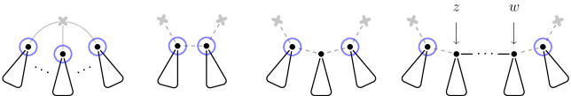
Figure 3. The graph $Q^{*}\coloneqq(Q-V(Q_{0}))-\mathcal{E}^{*}$. Vertices in $Q_{0}$ are crossed, edges in $\mathcal{E}^{*}$ are dashed, and vertices in $R$ are circled. (Edges incident with $V(Q_{0})$ are not present in $Q^{*}$.) Each component of $Q^{*}$ is a tree (coloured black).

$\blacktriangleright$Anatomy of $Q$. Let $Q_{1}\subseteq Q$ be the subdivided $Q_{0}$. We fix an arbitrary orientation of $Q$, writing $Q_{1}$ and $Q$ for both the oriented and underlying graphs. By relabelling if necessary, we may assume $V(Q_{0})=\{x_{1},\ldots,x_{q}\}$ is the set of vertices in $Q_{1}$ corresponding to vertices in $Q_{0}$. Note $V(Q_{0})$ is independent in $Q$, and every vertex whose underlying degree in $Q_{1}$ is strictly greater than $2$ lies in $V(Q_{0})$. For each $x_{i}x_{j}\in E(Q_{0})$, where $i<j$, let $P(ij)\subseteq Q_{1}$ be the path arising from the subdivision of $x_{i}x_{j}$, and let

$$\mathcal{E}\phantom{{}^{*}} \coloneqq\{(i,j):\text{ $i<j$ and $x_{i}x_{j}\in E(Q_{0})$ }\} R \coloneqq N_{Q}(V(Q_{0}))$$

$$\mathcal{E}^{*} \coloneqq\bigcup_{(i,j)\in\mathcal{E}}\{uv:\text{ $uv\in E(P(ij))$ and $\{u,v\}\cap R\neq\varnothing$}\} Q^{*} \coloneqq(Q-V(Q_{0}))-\mathcal{E}^{*}$$

Let $\mathcal{C}$ be the set of components of $Q^{*}$; note that each component $C\in\mathcal{C}$ of $Q^{*}$ is a tree. Following Lemma 4.1, we shall split trees with many bare paths into pieces. The procedure is a bit more technical here because we have many trees (of possibly quite distinct sizes) and some of them have two vertices with neighbours in the rest of $Q$. (See Figure 3.)

Our first goal is to select a collection $\mathcal{P}\subseteq\mathcal{P}_{Q}$ of bare paths and to fix a tree-partition of each component $C\in\mathcal{C}$ in such a way that the remaining steps of the proof can be carried out as in the proofs of Lemmas 4.1 and 4.2. As a preliminary step, for each tree component $C$ of $Q^{*}$ we fix a sequence of rooted trees $s(C)=(T_{i}^{C})_{i=1}^{m(C)}$, where $m(C)\in[4]$ forming a tree-partition of $C$ in each of the two following cases. Importantly, we shall guarantee that $\mathcal{P}$ is a large collection of paths whose middles are $\prec$-isomorphic (each tree will be adequately rooted), and that if some $C\in\mathcal{C}$ contains sufficiently many paths in $\mathcal{P}$, then $T_{1}^{C}$ contains many paths in $\mathcal{P}$ and $T_{2}^{C}$ is large. Also, each path in $\mathcal{P}$ shall lie in some $T_{1}^{C}$.

$\blacktriangleright$Tree-split if at most one vertex $y\in C$ has neighbours outside of $C$. Then either $y\in R$ or $y$ has precisely two distinct neighbours $r_{1},r_{2}\in R$ (and no neighbours in $Q_{0}$). If $C$ contains strictly less than $3\sqrt{\log n}$ bare paths of $\mathcal{P}_{Q}$, then let $s(C)=(Y,Y,C)$, where $Y\coloneqq(\{y\},\varnothing)$.

Suppose $C$ contains at least $3\sqrt{\log n}$ bare paths of $\mathcal{P}_{Q}$. Fix a tree partition $\{S,B\}$ of $C$ where $S$ contains at least $\sqrt{\log n}$ bare paths of $\mathcal{P}_{Q}$ and $|S|\leq|B|$, using Lemma 2.1. If $y\in S$, then let $s(C)=(S,B)$, where $S$ is rooted in $y$ and $B$ is rooted in the sole vertex in $V(S)\cap V(B)$. If $y\in B$, then let $r\neq y$ be the sole vertex in $V(S)\cap V(B)$, let $y^{\prime}$ be the neighbour of $r$ in the path from $y$ to $r$, and let $D\subseteq V(B)$ be the set of vertices consisting of $y^{\prime}$ and its descendants, considering $B$ rooted at $y$. Also, let $T_{y^{\prime}}$ (respectively $T_{r}$) be the tree component of $B[D]-y^{\prime}r$ which contains $y^{\prime}$ (resp. $r$). Note that $|B\smallsetminus D|+|T_{r}|+|T_{y^{\prime}}|=|B|\geq|C|/2$; we fix a tree-partition of $C$ as follows. If $|B\smallsetminus D|\geq|C|/6$, then fix a tree-partition $\{T_{1}^{C},T_{2}^{C},T_{3}^{C}\}$ of $C$ with $T_{1}^{C}=S\cup T_{r}$ and $T_{2}^{C}=B-D$, and let $s(C)=(T_{1}^{C},T_{2}^{C},T_{3}^{C})$; the roots of $T_{1}^{C}$, $T_{2}^{C}$ and $T_{3}^{C}$ are $r$, $y$ and $y^{\prime}$, respectively. If instead $|B\smallsetminus D|<|C|/6$ and $|T_{r}|\geq|C|/6$, then fix a tree-partition $\{T_{1}^{C},T_{2}^{C}\}$ of $C$ with $T_{2}^{C}=T_{r}$ and let $s(C)=(T_{1}^{C},T_{2}^{C})$, with $T_{1}^{C}$ rooted in $y$ and $T_{2}^{C}$ in $r$. Finally, if $|B\smallsetminus D|<|C|/6$ and $|T_{r}|<|C|/6$, then $|T_{y^{\prime}}|\geq|C|/6$, and we fix a tree-partition $\{T_{1}^{C},T_{2}^{C}\}$ of $C$ with $T_{2}^{C}=T_{y^{\prime}}$ and let $s(C)=(T_{1}^{C},T_{2}^{C})$, where $T_{1}^{C}$ has root $y$ and $T_{2}^{C}$ has root $y^{\prime}$. $\blacktriangleleft$

$\blacktriangleright$Tree-split if precisely two distinct vertices $z,w\in C$ have neighbours outside of $C$. In this case, each of $z,w$ has precisely one neighbour in $R$ (and no other neighbours outside of $C$, see Figure 3); moreover, $z$ and $w$ lie in a path $P(ij)$ for some $(i,j)\in\mathcal{E}$. For each subtree $T\subseteq C$, let $\omega(T)$ be the number of vertex-disjoint bare paths of $\mathcal{P}_{Q}$ in $T$ if $C$ contains at least $6\sqrt{\log n}$ such paths; otherwise, let $\omega(T)=|T|$. Let $T_{z}$ and $T_{w}$ be the components of $C-E(P(ij))$ containing $z$ and $w$, respectively, and let $C^{\prime}\coloneqq T-(T_{z}\cup T_{w})$. We may assume, without loss of generality, that $\omega(T_{w})<\omega(C)/2$. We fix a partition of $C\smallsetminus T_{w}$ as we would do in the previous case if the edge between $w$ and $V(C)\smallsetminus V(T_{w})$ did not exist (and taking the single neighbour of $z$ in $R$ as $y$); this yields a sequence of two or three trees, to which we append another one (consisting of $T_{w}$ plus the two edges connecting it to the rest of $C$ and to $R$), completing a tree-partition of $C$. $\blacktriangleleft$

We note that, if $C\in\mathcal{C}$ has $b_{C}\geq 3\sqrt{\log n}$ bare paths of $\mathcal{P}_{Q}$, then $T_{1}^{C}$ contains at least $b_{C}/3$ of these paths, otherwise it contains none. Moreover

(30) $$|T_{2}^{C}|\geq|C|/6\geq|T_{1}^{C}|/6.$$

For each $\mathcal{A}\subseteq\mathcal{P}_{Q}$ and each $C\in\mathcal{C}$, we define $\mathcal{A}(C)\coloneqq\{P\in\mathcal{A}:P\subseteq T_{1}^{C}\}$.

If $C\in\mathcal{C}$ and $|\mathcal{P}_{Q}(C)|=0$, then $|\mathcal{P}_{Q}(C)|\geq\max\bigl{\{}\,\sqrt{\log n},\,\bigl{|}\{P\in\mathcal{P}_{Q}:P\subseteq C\}\bigr{|}/6\,\bigr{\}}$. Moreover,

$$\Bigl{|}\bigcup_{C\in\mathcal{C}}\mathcal{P}_{Q}(C)\Bigr{|}>{\cramped{\frac{|\mathcal{P}_{Q}|}{7}}}.$$

Proof.

The first part of the claim follows immediately by the definition of $T_{1}^{C}$. Also, each $v\in Q_{0}\cup R$ lies in at most one $P\in\mathcal{P}_{Q}$, and if $C\in\mathcal{C}$ contains $b_{C}$ paths of $\mathcal{P}_{Q}$, then $\mathcal{P}_{Q}$ contains at most $\max\{6\sqrt{\log n},\,5b_{C}/6\}$ paths in $C$ which do not lie in $T_{1}^{C}$. Since $|\mathcal{C}|\leq|Q\cup R|\leq|Q_{0}|\Delta(Q)\leq\zeta n^{1/4}$ and $|\mathcal{P}_{Q}|=\lambda n$, we have

$$\Bigl{|}\bigcup_{C\in\mathcal{C}}\mathcal{P}_{Q}(C)\Bigr{|} \geq|\mathcal{P}_{Q}|-|Q_{0}\cup R|-|\mathcal{C}|6\sqrt{\log n}-\frac{5}{6}|\mathcal{P}_{Q}|\geq\frac{|\mathcal{P}_{Q}|}{7}.\qed$$

Let $\mathcal{F}^{\diamond}$ be the set of all $4$ nonisomorphic rooted oriented paths of order $3$. If $P\in\mathcal{P}_{Q}(T_{1}^{C})$ for some $C\in\mathcal{C}$, we consider $P$ rooted at (its endvertex which is) the latest common ancestor of $V(P)$ in $T_{1}^{C}$.

There exists $P_{\mathrm{ref}}\in\mathcal{F}^{\diamond}$ and a collection $\mathcal{P}\subseteq|\bigcup_{C\in\mathcal{C}}\mathcal{P}_{Q}(C)|$, with $|\mathcal{P}|\geq\lambda n/300$, such that

1. each $P\in\mathcal{P}$ is contained in precisely one $T_{1}^{C}$ and $V(P)\cap(V(Q)\smallsetminus T_{1}^{C})=\varnothing$;

2. if $P\subseteq\mathcal{P}(C)$, then $P$ does not contain the root of $T_{1}^{C}$;

3. for each $C\in\mathcal{C}$, either $|\mathcal{P}(C)|=0$ or $\sqrt{\log n}/9\leq|\mathcal{P}(C)|=\min\bigl{\{}|\mathcal{P}_{Q}(C)|,\bigl{\lceil}|T_{1}^{C}|/14\bigr{\rceil}\bigr{\}}\pm 1$;

4. $\operatorname{middle}(P)$ and $P_{\mathrm{ref}}$ are $\prec$-isomorphic for each $P\in\mathcal{P}$.

Proof.

We first select $\mathcal{P}_{Q}^{\prime}\subseteq\bigcup_{C\in\mathcal{C}}\mathcal{P}_{Q}(C)$ as follows. For each $C\in\mathcal{C}$, choose $\max\{0,|\mathcal{P}_{Q}(T_{1}^{C})|-\lceil|T_{1}^{C}|/14\rceil\}$ paths in $\mathcal{P}_{Q}(T_{1}^{C})$ arbitrarily and colour them red; then colour red every path in $\mathcal{P}_{Q}$ containing the root of some $T_{1}^{C}$. Let $\mathcal{P}_{Q}^{\prime}\coloneqq\{P\in\bigcup_{C\in\mathcal{C}}\mathcal{P}_{Q}(C):\text{$P$ has not been coloured}\}$. Clearly the paths in $\mathcal{P}_{Q}$ satisfy (2). Moreover, (1) holds because the elements of $\mathcal{C}$ are (vertex-disjoint) tree components of $Q^{*}$. If $|\mathcal{P}_{Q}^{\prime}(C)|>0$, then $|T_{1}^{C}|\geq 7|\mathcal{P}_{Q}(C)|$, so

(31) $$|\mathcal{P}_{Q}^{\prime}(C)|\pm 1=\min\left\{|\mathcal{P}_{Q}(C)|,\left\lceil\frac{|T_{1}^{C}|}{14}\right\rceil\right\}\geq\min\left\{|\mathcal{P}_{Q}(C)|,\frac{7|\mathcal{P}_{Q}(C)|}{14}\right\}=\frac{|\mathcal{P}_{Q}(C)|}{2}\geq\sqrt{\log n}/2,$$

where the last inequality is a consequence of Claim 6. By the same claim, we have

(32) $$|\mathcal{P}_{Q}^{\prime}|\geq|\mathcal{P}_{Q}|/14\geq\lambda n/14.$$

For each $C\in\mathcal{C}$, at least $|\mathcal{P}_{Q}^{\prime}(C)|/4$ paths in $\mathcal{P}_{Q}^{\prime}(C)$ have their middle $\prec$-isomorphic to some $P_{C}\in\mathcal{F}^{\diamond}$. So there exists $P_{\mathrm{ref}}\in\mathcal{F}^{\diamond}$ and $\mathcal{P}\coloneqq\{P\in\mathcal{P}_{Q}^{\prime}(C):\text{$\operatorname{middle}(P),P_{\mathrm{ref}}$ and\leavevmode\nobreak\ $P_{C}$ are $\prec$-isomorphic, $C\in\mathcal{C}$}\}$ such that $|\mathcal{P}|\geq|\mathcal{P}_{Q}^{\prime}|/16\geq\lambda n/300$, by (32). Clearly (1), (2) and (4) hold. Finally, note that if $\mathcal{P}(C)>0$, then $\mathcal{P}(C)\geq|\mathcal{P}_{Q}^{\prime}(C)/4$ so (3) holds by (31). ∎

Fix $P_{\mathrm{ref}}$ and $\mathcal{P}$ as in the claim. We fix a partition $\mathcal{C}=\mathcal{C}_{\text{path}}\mathbin{\dot{\cup}}\mathcal{C}_{\text{free}}$, where $\mathcal{C}_{\text{path}}\coloneqq\{C\in\mathcal{C}:\mathcal{P}(C)\neq\varnothing\}$. Roughly speaking, each $C\in\mathcal{C}_{\text{path}}$ contains a large number of bare paths in $T_{1}^{C}$ which are $\prec$-isomorphic to $P_{\mathrm{ref}}$. We say $C\in\mathcal{C}$ is $1$-grounded if precisely one vertex of $C$ has neighbours in $Q-C$, and call $C$ $2$-grounded otherwise. The vertices of $C$ with neighbours in $Q-C$ are its anchors. For each $T\in\mathcal{C}_{\text{path}}$, let $n_{C}\coloneqq|C|$ and fix a partition $\mathcal{P}_{C}\coloneqq\mathcal{P}(C)\coloneqq\mathcal{P}_{C}^{0}\mathbin{\dot{\cup}}\mathcal{P}_{C}^{H}\mathbin{\dot{\cup}}\mathcal{P}_{C}^{\diamond}$ with the following properties.

(33) $$\begin{aligned} |\mathcal{P}_{C}^{0}|&=|V_{0}|\frac{|\mathcal{P}_{C}|}{|\mathcal{P}|}\pm 1\\ \sum_{C\in\mathcal{C}_{\text{path}}}|\mathcal{P}_{C}^{0}|&=|V_{0}|\end{aligned} \begin{aligned} |\mathcal{P}_{C}^{H}|&\geq\lambda^{\prime}|\mathcal{P}_{C}|\\ \sum_{C\in\mathcal{C}_{\text{path}}}|\mathcal{P}_{C}^{H}|&\equiv 0\bmod k\end{aligned} \begin{aligned} |\mathcal{P}_{C}^{\diamond}|&\geq\lambda^{\prime}|\mathcal{P}_{C}|\\ \sum_{C\in\mathcal{C}_{\text{path}}}|\mathcal{P}_{C}^{\diamond}|&\equiv 0\bmod 2(k-1)\end{aligned}$$

(Recall that $\mathcal{P}_{C}$ contains only paths in $T_{1}^{C}$ whose middle is $\prec$-isomorphic to $P_{\mathrm{ref}}$.) We call the elements of $V(Q_{0})$ ground vertices and the elements of $R$ link vertices.

$\blacktriangleright$Final definition of $s(C)$. Abusing notation, we redefine $s(C)$ for each $C\in\mathcal{C}_{\text{free}}$ (but not for components in $\mathcal{C}_{\text{path}}$), applying again the tree-splitting procedure above, while replacing $\mathcal{P}_{Q}$ by $\mathcal{P}$ (in other words, we act as if $\mathcal{P}_{Q}$ contained no path $P$ with $P\subseteq C\in\mathcal{C}_{\text{free}}$). Of course, this means redefining $m(C)$ and $T_{m}^{C}$ for $C\in\mathcal{C}_{\text{free}}$ as well. Note that since $\mathcal{P}$ contains no path in any $C\in\mathcal{C}_{\text{free}}$, Claim 6 is not affected. $\blacktriangleleft$

$\blacktriangleright$Reduced graph. As in the proofs of Lemmas 4.2 and 5.2, we construct a regular partition of $G$. Introduce constants $d,\eta$ with $1/n\ll 1/K\ll\zeta\ll 1/k\ll\varepsilon\ll d\ll\lambda^{\prime}\ll\lambda\ll\eta\ll\alpha$ and apply Lemma 2.7 to obtain a partition $V_{0}\mathbin{\dot{\cup}}V_{1}\mathbin{\dot{\cup}}\cdots\mathbin{\dot{\cup}}V_{k}$ and a digraph $R^{\star}$ with $V({R^{\star}})=V_{0}\mathbin{\dot{\cup}}[k]$; moreover we may assume that $H=1{\color[rgb]{0,0,0}\to}2\cdots{\color[rgb]{0,0,0}\to}\cdots{\color[rgb]{0,0,0}\to}k{\color[rgb]{0,0,0}\to}1$ is a Hamilton cycle in ${R^{\star}}[[k]]$. By Lemma 1, ${R^{\star}}[[k]]$ contains a spanning subgraph $H^{\diamond}$ which is $P_{\mathrm{ref}}$-connected and such that $\Delta^{0}(H^{\diamond})\leq 4/\alpha$. Finally, it is not difficult to show that ${R^{\star}}[[k]]$ contains a subgraph $H^{4}$ of order at most $4$, with $1\in H^{4}$, and such that every rooted oriented cycle of length at most $3$ admits a homomorphism into $H^{4}$ in which the root is mapped to $1$ (see Figure 4). By Lemma 2.10, ${R^{\star}}[[k]]$ contains a $(25k^{2/3}/\eta)$-regular expander $J$, with $H\cup H^{\diamond}\cup H^{4}\subseteq J$. $\blacktriangleleft$

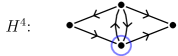
Figure 4. The digraph $H^{4}\subseteq{R^{\star}}[[k]]$, with $E(H^{4})=\{1u,u1,u\ell,\ell 1,1r,ur\}$. Vertex $1$ is marked. Every oriented path with at most $3$ arcs admits a homomorphism to $H^{4}$ mapping both of its leaves to $1$.

$\blacktriangleright$Allocation. We define a homomorphism $\varphi:Q\to J$ in three steps. Firstly we allocate the subgraph induced by ground vertices and their neighbours to $H^{4}$. Secondly, for each $m\in[4]$ in ascending order, we allocate $T_{m}^{C}$ to ${R^{\star}}$ (if $m(C)\leq m$) for all $C\in\mathcal{C}$. Finally the resulting map is slightly retouched. The allocation thus obtained will satisfy the following properties (as in Lemma 4.1, with the addition of (viii) below). There exist a tidy ancestral order $\prec_{T}$ of each $T\in\mathcal{C}$ and disjoint subsets $\mathcal{P}^{0},\mathcal{P}^{H}$ of $\mathcal{P}$ such that

1. $\Delta(\varphi)\leq 6$;

2. $|\mathcal{P}^{0}|=|V_{0}|$ and for each $P\in\mathcal{P}^{0}$ the centre of $P$ is mapped to $V_{0}$;

3. $\varphi$ maps precisely one vertex of $Q$ to each $v\in V_{0}$;

4. $\varphi$ maps at least $\lambda^{\prime}n/k$ centres of paths in $\mathcal{P}^{H}$ to each $i\in[k]$;

5. For each $i\in[k]$ we have $\bigl{|}\varphi^{-1}(i)\cap\{\,N_{T}^{-}(x)\cup N_{T}^{+}(x):\varphi(x)\in V_{0}\,\}\bigr{|}\leq 2\varepsilon n/\alpha k$;

6. For each $P\in\mathcal{P}^{H}$, the restriction of $\varphi$ to $\operatorname{middle}(P)$ is a homomorphism from $\operatorname{middle}(P)$ to $H$;

7. $\bigl{|}\varphi^{-1}(1)\bigr{|}=\bigl{|}\varphi^{-1}(2)\bigr{|}=\cdots=\bigl{|}\varphi^{-1}(k)\bigr{|}$.

8. For each $x\in Q_{0}$ and each $y\in N_{Q}(x)$ we have $\varphi(x)=1$ and $\varphi(y)\in H^{4}$.

–A-0. We shall allocate $Q[V(Q_{0})\mathbin{\dot{\cup}}R]$. Set $\varphi(x)=1$ for each $x\in Q_{0}$. Note that $Q[V(Q_{0})\mathbin{\dot{\cup}}R]$ is the union of edge-disjoint oriented paths of length at most $3$ joining vertices in $V(Q_{0})$. For each $i<j$ such that $P(ij)$ has length at most $3$, we extend $\varphi$ with the unique homomorphism $\varphi_{ij}$ from $P(ij)$ to $H^{4}$. Next, for each $y^{-}\in N_{Q}(Q_{0})$ whose image has not yet been defined, set $\varphi(y^{-})=j^{-}$ where $j^{-}\in N^{-}_{H^{4}}(1)$ arbitrarily, and proceed analogously for each $y^{+}\in N_{Q}(Q_{0})$.

–A-1 ($m=1$). Suppose first that $C\in\mathcal{C}_{\text{free}}$. We allocate $T_{1}^{C}$ to $R^{\star}$ using Algorithm 1, with the following changes. If $C$ has a single anchor $y$, then either $y\in R$ (in which case $y$ has already been allocated) or $y$ has precisely two neighbours $z,z^{\prime}\in R$. Fix a vertex ${j\in[k]}$ so that $\varphi(y)=j$ is a homomorphism of the (oriented) path $zyz^{\prime}\subseteq Q$. Finally, apply Algorithm 1 (unmodified) to obtain a homomorphism from $T_{1}^{C}$ to $J$. If $C$ has two anchors $z,w$, then $T_{1}^{C}=(\{y\},\varnothing)$ with $y\in R$ and there is nothing to do (recall $C\in\mathcal{C}_{\text{free}}$). Let us also check that not too many vertices are allocated to each $i\in[k]$. At most $|Q_{0}\mathbin{\dot{\cup}}R|\leq|Q_{0}|\Delta(Q)\leq\zeta n^{1/4}$ vertices were allocated in step A-0. Moreover $|\mathcal{C}|\leq|Q_{0}\mathbin{\dot{\cup}}R|$ so

$$\sum_{\begin{subarray}{c}C\in\mathcal{C}_{\text{free}}\\ |T_{1}^{C}|<\sqrt{\log n}\end{subarray}}|T_{1}^{C}|<|\mathcal{C}|\sqrt{\log n}=\zeta n^{3/4}.$$

If $C\in\mathcal{C}_{\text{free}}$ and $|T_{1}^{C}|\geq\sqrt{\log n}$, then at most $|T_{1}^{C}|(\frac{1}{k}\pm 1/|T_{1}^{C}|^{\mathrm{o}(1)})$ vertices of $T_{1}^{C}$ are allocated to each $i\in[k]$ by Lemma 3.1 (d).

Now suppose that $C\in\mathcal{C}_{\text{path}}$. If $C$ has a single anchor $y\in R$, allocate the root $r$ of $T_{1}^{C}$ as follows. If $r=y$, then $r$ has been allocated (to some $j\in[k]$) and there have nothing to do; if $r$ is a neighbour of $y$, allocate $r$ to an appropriate neighbour of $\varphi(y)$ in $[k]$; otherwise allocate $r$ to $j\in[k]$ chosen uniformly at random (this could also be done arbitrarily). We then proceed to define maps $\varphi_{0},\varphi_{H},\varphi_{\diamond}$ as in the setup phase of Lemma 4.1, (where $\mathcal{P}^{0},\mathcal{P}^{H},\mathcal{P}^{\diamond}$ there correspond to the union of the corresponding sets $\mathcal{P}_{C}^{0},\mathcal{P}_{C}^{H}$ or $\mathcal{P}_{C}^{\diamond}$ over all $C\in\mathcal{C}_{\text{path}}$, but following (33)). We map $T_{1}^{C}$, applying Algorithm 1 to the tree we obtain contracting paths in $\mathcal{P}_{C}^{0}\mathbin{\dot{\cup}}\mathcal{P}_{C}^{H}\mathbin{\dot{\cup}}\mathcal{P}_{C}^{\diamond}$ and greedily complete the allocation of these paths, following of Phase 1 of Lemma 4.1. In particular, the middles of paths in $\mathcal{P}^{\diamond}$ are evenly mapped along the $H^{\diamond}$, with at least $\lambda^{\prime}\mathcal{P}_{C}/2(k-1)$ middles mapped to each branch of a $P_{\mathrm{ref}}$  diamond, see (33). We argue similarly if $C$ has two anchors.

Crucially, since $\sqrt{\log n}\leq|T_{1}^{C}|\leq 12|T_{2}^{C}|$, the allocation algorithm maps roughly the same number of vertices of each $C\in\mathcal{C}_{\text{path}}$ to each $i\in[k]$, with preimage sizes differing in a value which is at most $72|T_{2}^{C}|/\eta k$ (this is essentially the bound (18), using $|\mathcal{P}(C)|\leq|C|/14$ and considering as $\varrho$ the combination of the allocation in the previous step and the homomorphisms of all $T_{1}^{C}$ over all $C\in\mathcal{C}_{\text{path}}$). Let $W_{1}\coloneqq V(Q_{0})\cup R\cup\bigcup_{C\in\mathcal{C}}V(T_{1}^{C})$. Note that every vertex of $V_{0}$ is the image of some vertex of $Q$. Since $|C|\geq\sqrt{\log n}$ for each $C\in\mathcal{C}_{\text{path}}$, the number of vertices so far allocated to each ${i\in[k]}$ is

$$\Bigl{|}\varrho^{-1}(i)\cap W_{1}\Bigr{|} =\pm\overbracket{\vphantom{\Bigl{(}\frac{|}{|}}2\zeta n^{3/4}}^{\text{\footnotesize\rule{0.0pt}{8.00002pt}$(*)$}}+\sum_{C\in\mathcal{C}_{\text{path}}}\overbracket{\vphantom{\left(\frac{|}{|}\right.}(|T_{1}^{C}|-|\mathcal{P}_{C}^{0}|)\Bigl{(}\frac{1}{k}\pm\frac{1}{(|T_{1}^{C}|/2)^{\mathrm{o}(1)}}\Bigr{)}}^{\text{\footnotesize\rule{0.0pt}{8.00002pt}$T_{1}^{C}$ without paths in\leavevmode\nobreak\ $\mathcal{P}(C)$}}\pm\overbracket{\vphantom{\left(\frac{|}{|}\right.}\frac{72}{\eta k}\Bigl{(}\sum_{C\in\mathcal{C}_{\text{path}}}|T_{2}^{C}|\Bigr{)}}^{\text{\footnotesize\rule{0.0pt}{8.00002pt}$\mathcal{P}(C)$}}$$

(34) $$=\frac{|W_{1}|-|V_{0}|}{k}\pm\frac{75}{\eta k}\Bigl{(}\sum_{C\in\mathcal{C}_{\text{path}}}|T_{2}^{C}|\Bigr{)},$$

Where the term $(*)$ corresponds to the allocation of $V(Q_{0})\mathbin{\dot{\cup}}R$ and each $T_{1}^{C}$ where $C\in\mathcal{C}_{\text{free}}$.

–A-1 ($m=2$). For each $C\in\mathcal{C}$ we allocate $T_{2}^{C}$ as follows. (This step corresponds to Phase 2 of Lemma 4.1, applied to $T_{2}^{C}$ for each $C\in\mathcal{C}_{\text{path}}$.) If $C\in\mathcal{C}_{\text{free}}$ then $T_{2}^{C}$ is a single vertex which has already been allocated, and we may therefore suppose $C\in\mathcal{C}_{\text{path}}$. Note that $|T_{2}^{C}|\geq|C|/12>\sqrt{\log n}/20$ by (30) and (3). The allocation up to this point may has used clusters quite unevenly (i.e., linear ‘imbalances’). Let $\varrho_{1}$ denote the homomorphism of $T_{1}^{C}$. If the root $r$ of $T_{2}^{C}$ has yet to be allocated, then $C$ is $1$-grounded and $r$ is the anchor of $C$; moreover, $r$ has precisely two neighbours $x,y$ in $R$. We set $\varrho_{1}(r)$ to a vertex ${j\in[k]}$ in the appropriate intersection of neighbourhoods of $x$ and $y$. For each $i\in[k]$, define, as in (19), the following

(35) $$\alpha_{i} \coloneqq\frac{1}{n_{2}}\left(\frac{n_{T}-n_{0}}{k}-|\varrho_{1}^{-1}(i)|+[i=j]\right)\qquad\text{and}\qquad b_{i}\coloneqq\alpha_{i}\log\log\log n_{2},$$

Where $n_{1}=|T_{1}^{C}|$, $n_{2}=|T_{2}^{C}|$ and $n_{T}=|V(T_{1}^{C})\cup V(T_{2}^{C})|$. As in (20) we have $\sum_{{i\in[k]}}\alpha_{i}=1$. We obtain an allocation $\varrho_{2}$ of $T_{2}^{C}$ using an auxiliary graph which is a weighted blow-up of $J$ (as in Lemma 4.1). We can follow the calculations in (21), (22), and (23) (with relabelled variables) to conclude that $\varrho_{T}=\varrho_{1}\lor\varrho_{2}$ is an allocation of $T\coloneqq T_{1}^{C}\cup T_{2}^{C}$ such that for each $i\in[k]$

$$|\varrho_{T}^{-1}(i)|=\frac{|T|-n_{0}}{k}\left(1\pm\frac{\log\log\log|T_{2}^{C}|}{|T_{2}^{C}|^{\mathrm{o}(1)}}\right).$$

Let $W_{2}\coloneqq V(Q_{0})\cup R\cup\bigcup_{C\in\mathcal{C}}V(T_{1}^{C}\cup T_{2}^{C})$. By (34), the allocation $\varrho_{\text{A-1}}$ obtained so far satisfies the following.

(36) $$\Bigl{|}\varrho_{\text{A-1}}^{-1}(i)\cap W_{2}\Bigr{|}=\frac{|W_{2}|-|V_{0}|}{k}\pm\sum_{C\in\mathcal{C}_{\text{path}}}\bigl{(}|T_{1}^{C}|-|\mathcal{P}_{C}^{0}|\bigr{)}\frac{\log\log\log|T_{2}^{C}|}{k|T_{2}^{C}|^{\mathrm{o}(1)}}=\frac{|W_{2}|-|V_{0}|}{k}\pm n^{1-\mathrm{o}(1)}$$

Where we use that $\pm\bigl{(}|T_{1}^{C}|-|\mathcal{P}_{C}^{0}|\bigr{)}\frac{\log\log\log|T_{2}^{C}|}{k|T_{2}^{C}|^{\mathrm{o}(1)}}=\pm|T_{2}^{C}|^{1-\mathrm{o}(1)}$ for each $C\in\mathcal{C}_{\text{path}}$, and that that $x\mapsto x^{c}$ is a concave concave function if $0<c<1$.

–A-1 ($m=3,4$). For each $C\in\mathcal{C}$ and $m\in[m(C)]\smallsetminus\{1,2\}$, we allocate $T_{m}^{C}$ as we did for components in $\mathcal{C}_{\text{free}}$ with one anchor. (Note that $T_{m}^{C}$ has precisely two neighbours already allocated.) Similarly, we can argue that the vertices of $T_{m}^{C}$ are either well-distributed or introduce a very small error in the allocation. More precisely, the combined error introduced by trees with at most $n^{1/5}$ vertices, is $\pm|Q_{0}|\Delta(Q)n^{1/5}=\pm\mathrm{o}(n^{2/3})$; while the combined error introduced by trees with at least $n^{1/5}$ vertices is $\pm|Q_{0}|\Delta(Q)/kn^{\mathrm{o}(1)/5}=\pm\mathrm{o}(n^{2/3})$.

Hence, it is not difficult to check that the combined homomorphism $\varrho$ constructed so far satisfies all properties (i)–(viii) except perhaps for (vii). Moreover if $\varrho$ is the homomorphism obtained thus far, then for each $i\in[k]$

$$|\varrho_{\text{A-1}}^{-}1(i)|=\frac{|Q|-|V_{0}|}{k}\pm n^{1-\mathrm{o}(1)}.$$

We correct these imbalances in the last stage of the allocation.

–A-2. Modify the allocation to satisfy (vii), using $P_{\mathrm{ref}}$-diamonds as in the proof of Lemma 4.1 (recall that each branch of each $P_{\mathrm{ref}}$-diamond in $H^{\diamond}$ is the image of $\lambda^{\prime}|\mathcal{P}_{C}|/2(k-1)\geq n/k^{2}$ middles of bare paths, by (33)), and let $\varphi$ be the final homomorphism, which satisfies all properties (i)–(viii). $\blacktriangleleft$

$\blacktriangleright$Embedding. The embedding follows closely the argument in Lemma 4.2. For the sake of brevity, we outline the argument, highlighting the main differences. Vertices are embedded in an order similar to the one in which they were allocated, except for the middles of paths in $\mathcal{P}^{H}$, which are embedded with perfect matchings.

We begin by reserving vertices for each $v\in V(Q_{0})\cup R$ using Lemma 2.7. (In particular, the requirement that $|Q_{0}|\leq\zeta n^{1/4}$ is due to the bounds in Lemmas 2.7 and 2.7.) We also reserve vertices which will be important for the final matching and when connecting middles of bare paths to exceptional vertices.

Next we embed the vertices in $V(Q_{0})\cup R$, and then proceed to embed the trees $T_{m}^{C}$ for each $C\in\mathcal{C}$ and each $m\in m(C)$. Each tree is almost completely embedded before we start embedding the next (the exception being the middles of bare paths in $\mathcal{P}^{H}$). Moreover, each tree is embedded in a tidy ancestral order, which ensures we do not reserve too many vertices at any point. The embedding algorithm never runs out of room since, as in Lemma 4.2 we have yet to embed the centres of bare paths in $\mathcal{P}^{H}$, and these were uniformly allocated over $[k]$. We complete the embedding with perfect matchings, using some sets reserved at the beginning to ensure superregularity, as in Lemma 4.2. ∎

References

- [1] N. Alon, R. A. Duke, H. Lefmann, V. Rödl, and R. Yuster. The algorithmic aspects of the regularity lemma. Journal of Algorithms, 16(1):80–109, 1994.
- [2] J. Balogh, B. Csaba, and W. Samotij. Local resilience of almost spanning trees in random graphs. Random Structures & Algorithms, 38(1-2):121–139, 2011.
- [3] J. A. Bondy and U. S. R. Murty. Graph theory, volume 244 of Graduate Texts in Mathematics. Springer-Verlag, New York, 2008.
- [4] J. Böttcher, J. Han, Y. Kohayakawa, R. Montgomery, O. Parczyk, and Y. Person. Universality for bounded degree spanning trees in randomly perturbed graphs. Random Structures & Algorithms, 55(4):854–864, 2019.
- [5] J. Böttcher, M. Schacht, and A. Taraz. Proof of the bandwidth conjecture of Bollobás and Komlós. Mathematische Annalen, 343(1):175–205, 2009.
- [6] D. Clemens, A. Ferber, R. Glebov, D. Hefetz, and A. Liebenau. Building spanning trees quickly in maker-breaker games. SIAM Journal on Discrete Mathematics, 29(3):1683–1705, 2015.
- [7] L. DeBiasio, D. Kühn, T. Molla, T. Osthus, and A. Taylor. Arbitrary orientations of hamilton cycles in digraphs. SIAM Journal on Discrete Mathematics, 29(3):1553–1584, 2015.
- [8] L. DeBiasio and T. Molla. Semi-degree threshold for anti-directed Hamiltonian cycles. Electronic Journal of Combinatorics, 22(4), 2015.
- [9] R. Diestel. Graph theory, volume 173 of Graduate Texts in Mathematics. Springer-Verlag, New York, 1997. Translated from the 1996 German original.
- [10] M. A. Ghouila-Houri. Une condition suffisante d’existence d’un circuit Hamiltonien. Comptes Rendus de l’Académie des Sciences, 25:495–497, 1960.
- [11] S. Janson, T. Łuczak, and A. Ruciński. Random graphs. Wiley-Interscience, New York, 2000.
- [12] J. Komlós, G. N. Sárközy, and E. Szemerédi. Proof of a packing conjecture of Bollobás. Combinatorics, Probability, and Computing, 4(3):241–255, 1995.
- [13] J. Komlós, G. N. Sárközy, and E. Szemerédi. Spanning trees in dense graphs. Combinatorics, Probability, and Computing, 10:397–416, 2001.
- [14] M. Krivelevich, M. Kwan, and B. Sudakov. Bounded-degree spanning trees in randomly perturbed graphs. SIAM J. Discrete Math., 31(1):155––171, 2017.
- [15] D. Kühn, R. Mycroft, and D. Osthus. An approximate version of Sumner’s universal tournament conjecture. Journal of Combinatorial Theory, Series B, 101(6):415–447, 2011.
- [16] C. McDiarmid. Concentration. In Probabilistic methods for algorithmic discrete mathematics, volume 16 of Algorithms Combin., pages 195–248. Springer, Berlin, 1998.
- [17] J. W. Moon. Counting labelled trees. Number 1 in Canadian Mathematical Monographs. Canadian Mathematical Congress, 1970.
- [18] R. Mycroft and T. Naia. Unavoidable trees in tournaments. Random Structures & Algorithms, 53(2):352–385, 2018.
- [19] B. Sudakov and J. Vondrák. A randomized embedding algorithm for trees. Combinatorica, 30(4):445–470, 2010.
- [20] E. Szemerédi. On sets of integers containing no elements in arithmetic progression. Acta Arith., 27:199–245, 1975. Collection of articles in memory of Juriĭ Vladimirovič Linnik.
- [21] E. Szemerédi. Regular partitions of graphs. In Problèmes combinatoires et théorie des graphes (Colloq. Internat. CNRS, Univ. Orsay, Orsay, 1976), pages 399–401. CNRS, Paris, 1978.