On the two-dimensional quantum confined Stark effect in strong electric fields

Abstract.

We consider a Stark Hamiltonian on a two-dimensional bounded domain with Dirichlet boundary conditions. In the strong electric field limit we derive, under certain local convexity conditions, a three-term asymptotic expansion of the low-lying eigenvalues. This shows that the excitation frequencies are proportional to the square root of the boundary curvature at a certain point determined by the direction of the electric field.

1. Introduction

1.1. Physical motivation

There has been a lot of theoretical and experimental work on the properties of quantum confined semiconductor devices. These systems exhibit interesting features that may find applications in nano-technology (see e.g. [9, 10]). Physically, the confinement may be achieved through an interface with the vacuum or an hetero-junction, i.e., by interfacing the semiconductor with an isolator or with another semiconductor of larger gap [9]. The most prominent semiconductor devices are the so-called quantum wells, quantum wires and quantum dots, where the material is confined in one, two and three orthogonal directions, respectively. In the presence of symmetry along the non-confined directions the description of the system is reduced to the study of a Hamiltonian in dimension one, for quantum wells, and in dimension two for quantum wires (see e.g., [9, Chapter 8]).

An interesting phenomenon is the behavior of the energy levels of the system when a uniform electric field is applied; this is known as the quantum confined Stark effect [16] (see also [19] and references therein). In a simplified model one may consider independently electrons or holes. Then, in the so-called effective mass envelope function approximation [17], the effective Hamiltonian describing the quantum confined Stark effect is formally given by

$$-\frac{\hbar^{2}}{2m}\Delta+q\,{\mathbf{F}}\cdot{\mathbf{x}}+V_{\rm conf}\,,$$ (1.1)

where $\hbar$ is Plank’s constant divided by $2\pi$, $m>0$ is the effective mass of the electron (or hole), $-q$ is the charge of the particle (electron or hole), ${\mathbf{F}}$ is the electric field, and $V_{\rm conf}$ is some confining potential. In the simplest case one models the confining potential as infinite potential walls, i.e., one considers the first two terms of the Hamiltonian in (1.1) restricted to the domain of confinement with Dirichlet boundary conditions. The quantum confined Stark effect modeled as in (1.1) with Dirichlet boundary conditions have been considered, for instance, in [5, 16] for quantum wells, in [21, 23, 25, 22, 14, 10] for quantum wires, and in [24, 19] for quantum dots.

In this work we are interested in the study of the low-lying eigenvalues of the following two-dimensional Hamiltonian restricted to an open set $\Omega\subset\mathbb{R}^{2}$:

$$H=-\frac{\hbar^{2}}{2m}(\partial_{x}^{2}+\partial_{y}^{2})+q{F}x\,,$$ (1.2)

acting on a dense subspace of the square integral functions $L^{2}(\Omega)$ with Dirichlet boundary conditions. This is a model Hamiltonian to describe the energy levels of a quantum wire with cross section $\Omega$ in the presence of an electric field perpendicular to the non-confined direction. Notice that we have chosen coordinates such that ${\mathbf{F}}$ is parallel to the $x$-axis.

The low-lying eigenvalues of this operator have been studied, partially numerically, for different geometries in several papers such as in [21, 23] for squares, in [25] for rectangles, in [22, 14, 18] for disks, and in [10] for annuli.

From now on we will work with domains satisfying the following conditions, see Figure 1.

Assumption 1.1.

The set $\Omega$ is open, bounded, and connected. We assume that there exists a unique point $A_{0}\in\partial\Omega$ such that the first component of $A_{0}$ is given by

$$x_{\min}=\inf_{(x,y)\in\Omega}x=\min_{(x,y)\in\overline{\Omega}}x\,.$$

We also assume that $\partial\Omega$ is smooth near $A_{0}$, and that the curvature at $A_{0}$, denoted by $\kappa_{0}$, is positive.

Let us describe the notion of curvature we use in this paper. Consider a smooth counterclockwise parametrization $s\mapsto\gamma(s)$ by arc-length of the boundary near $A_{0}=\gamma(0)$. If ${\boldsymbol{n}}(s)$ is the outward pointing normal to $\partial\Omega$ at $\gamma(s)$, the curvature $\kappa(s)$ at $\gamma(s)$ is defined through the relation $\gamma^{\prime\prime}(s)=-\kappa(s){\boldsymbol{n}}(s)$. We have $\kappa(0)=\kappa_{0}>0$.

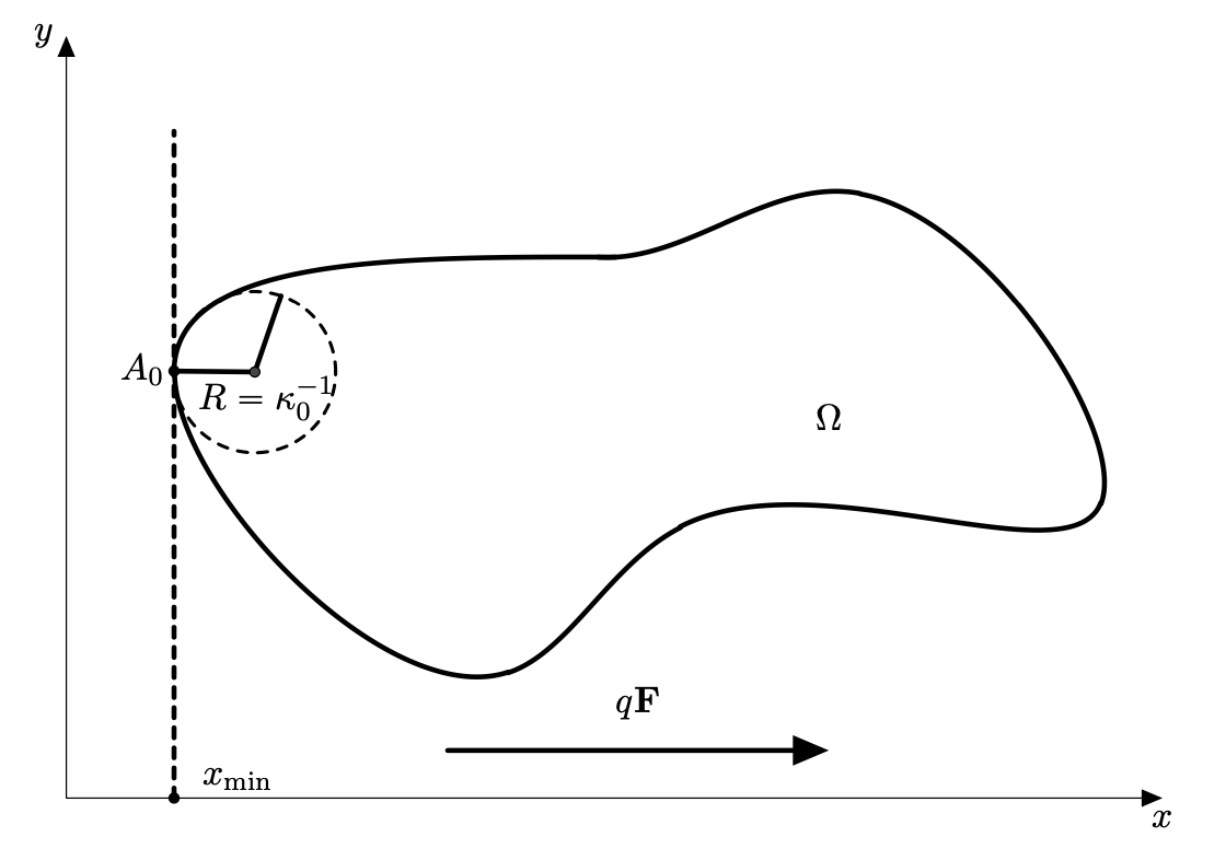
Figure 1. The domain $\Omega$.

Then we can provide a three terms asymptotic expansion for the individual eigenvalues of $H$ in the limit of strong electric fields. Our main result, Theorem 1.2, implies that for $qF>0$ the $n$-th eigenvalue of $H$ behaves in the limit of strong electric field as

$$E_{n}=qFx_{\rm min}+\left(\frac{(qF\hbar)^{2}}{2m}\right)^{\frac{1}{3}}z_{1}+(n-\tfrac{1}{2})\hbar\left(\frac{qF\kappa_{0}}{m}\right)^{\frac{1}{2}}+\mathscr{O}(F^{1/3})\,,$$ (1.3)

where $z_{1}\approx 2.338$ is the absolute value of the smallest zero of the Airy function.

In particular, we find an interesting behaviour of the energy splitting in terms of the geometry of $\Omega$ which is proportional to the $F^{1/2}$. Such an equidistant splitting for the eigenvalues in the strong electric field regime has been observed in [14] for disk shaped $\Omega$ using partially numerical methods (see Figure 7 from [14]). However, its dependence on the curvature does not seem to have been reported before. Heuristically the third term in the expansion may be explained as follows: under a strong electric field the particle is pushed towards $x_{\rm min}$ and behaves as an harmonic oscillator in the direction perpendicular to the field with elastic constant proportional to the curvature at $x_{\rm min}$. Let us mention here that a physics-oriented paper is in preparation. Our first investigations in this direction suggest that the spectral splitting (1.3) might be experimentally accessible.

1.2. Main result

Let $\Omega$ be as in Assumption 1.1. Notice that by factorizing $qF>0$ in the expression of $H$ in (1.2) we have

$$\mathscr{L}_{h}:=(qF)^{-1}H=-h^{2}(\partial^{2}_{x}+\partial^{2}_{y})+x\,,\quad h=\frac{\hbar}{\sqrt{2mqF}}\,.$$ (1.4)

We define $\mathscr{L}_{h}$ as the unique self-adjoint operator defined through the quadratic form

$$\mathscr{Q}_{h}(\varphi)=h^{2}\int_{\Omega}\left|\nabla\varphi(x)\right|^{2}\mathrm{d}x+\int_{\Omega}x\left|\varphi(x)\right|^{2}\mathrm{d}x\,,\quad\varphi\in H^{1}_{0}(\Omega)\,.$$

The operator $\mathscr{L}_{h}$ has domain contained in $H^{1}_{0}(\Omega)$ and acts as in (1.4). This is the Dirichlet realization of the Stark Hamiltonian. We want to describe the first eigenvalues of this operator in the limit $h\to 0$. We obtain (1.3) from the following result. Denote by $(\lambda_{n}(h))_{n\geq 1}$ the eigenvalues of $\mathscr{L}_{h}$ in increasing order, where each eigenvalue is repeated according to its multiplicity.

Theorem 1.2.

Let $n\in\{1,2,\dots\}$. Then, we have as $h\to 0$

$$\lambda_{n}(h)=x_{\min}+z_{1}h^{\frac{2}{3}}+h(2n-1)\sqrt{\frac{\kappa_{0}}{2}}+\mathscr{O}(h^{\frac{4}{3}})\,.$$

Remark 1.3.

Various extensions of our main theorem can be considered.

1. It is possible to prove asymptotic expansions in powers of $h^{1/6}$ of the low-lying eigenvalues by using a formal series analysis.

2. In our generic geometric situation, we could even prove that the eigenfunctions admit WKB expansions.

3. Our strategy may be adapted to deal with a finite number of non-degenerate minima, and it would even be possible to investigate tunnel effects when these minima have symmetries.

The proofs of such extensions can be adapted from a recent literature developed in the context of the Born-Oppenheimer approximation (see for instance [20, Chapter 11], or the generalizations [13, 15], and also [11] where tunnelling estimates are also considered).

Remark 1.4.

If we replace the potential $x$ by $ix$ in the Hamiltonian and one looks at the real part of the eigenvalues the second term in the asymptotic expansion has a factor $1/2$ (see e.g., [7, 12, 4, 1]). Concerning the analysis in the case of imaginary electric fields, the reader might also want to consider [8, 2, 3].

The rest of this article is organized as follows: In Section 2 we show that low energy eigenfunctions and its derivatives are exponentially well localized around $x_{\min}$. We use this to find an effective Hamiltonian $\widetilde{\mathscr{M}}_{h}$, whose low energy eigenvalues are those of $H$ modulo an exponentially small error, this is done in Section 3. This operator is expressed in tubular coordinates and acts on a tiny domain around $x_{\rm min}$ with Dirichlet boundary conditions. In the last section we provide asymptotic upper and lower bounds for the eigenvalues of $\widetilde{\mathscr{M}}_{h}$.

2. Localization near the potential minimum

The following proposition states that the eigenfunctions associated with the low-lying eigenvalues are localized in $x$ near $x_{\min}$.

Proposition 2.1.

Let $M>0$. There exist $\varepsilon,C,h_{0}>0$ such that, for all $h\in(0,h_{0})$, for all eigenvalues $\lambda$ such that $\lambda\leq x_{\min}+Mh^{\frac{2}{3}}$, and all corresponding eigenfunctions $\psi$,

$$\int_{\Omega}e^{\varepsilon|x-x_{\min}|^{\frac{3}{2}}/h}|\psi|^{2}\mathrm{d}{\bf x}\leq C\|\psi\|^{2}\,,$$ (2.1)

and

$$\int_{\Omega}e^{\varepsilon|x-x_{\min}|^{\frac{3}{2}}/h}|h\nabla\psi|^{2}\mathrm{d}{\bf x}\leq Ch^{2/3}\|\psi\|^{2}\,.$$ (2.2)

Proof.

We write the Agmon formula, for all $\psi\in\mathrm{Dom}(\mathscr{L}_{h})$ and all bounded Lipschitz functions $\Phi$:

$$\langle\mathscr{L}_{h}\psi,e^{2\Phi/h}\psi\rangle=\mathscr{Q}_{h}(e^{\Phi/h}\psi)-\|e^{\Phi/h}\nabla\Phi\psi\|^{2}\,.$$

Let $\psi$ be an eigenfunction corresponding to an eigenvalue $\lambda\leq x_{\min}+Mh^{\frac{2}{3}}$. We get

$$\int_{\Omega}h^{2}|\nabla e^{\Phi/h}\psi|^{2}+(x-\lambda-|\nabla\Phi|^{2})|e^{\Phi/h}\psi|^{2}\mathrm{d}x\mathrm{d}y=0\,,$$ (2.3)

and thus

$$\int_{\Omega}h^{2}|\nabla e^{\Phi/h}\psi|^{2}+(x-x_{\min}-Mh^{2/3}-|\nabla\Phi|^{2})|e^{\Phi/h}\psi|^{2}\mathrm{d}x\mathrm{d}y\leq 0\,.$$ (2.4)

Now, we choose $\Phi=\varepsilon|x-x_{\min}|^{3/2}$ and drop the first term above to get that

$$\int_{\Omega}\left(\left(1-\frac{9}{4}\varepsilon^{2}\right)(x-x_{\min})-Mh^{2/3}\right)|e^{\Phi/h}\psi|^{2}\mathrm{d}x\mathrm{d}y\leq 0\,.$$

We take $\varepsilon$ such that $1-\frac{9}{4}\varepsilon^{2}>0$ and fix $R>0$ such that

$$\left(1-\frac{9}{4}\varepsilon^{2}\right)R-M=1\,.$$ (2.5)

We write

$$\int_{|x-x_{\min}|\geq Rh^{2/3}}\left(\left(1-\frac{9}{4}\varepsilon^{2}\right)(x-x_{\min})-Mh^{2/3}\right)|e^{\Phi/h}\psi|^{2}\mathrm{d}x\mathrm{d}y\\ \leq-\int_{|x-x_{\min}|<Rh^{2/3}}\left(\left(1-\frac{9}{4}\varepsilon^{2}\right)(x-x_{\min})-Mh^{2/3}\right)|e^{\Phi/h}\psi|^{2}\mathrm{d}x\mathrm{d}y\,,$$

and get (using (2.5)):

$$h^{2/3}\int_{|x-x_{\min}|\geq Rh^{2/3}}|e^{\Phi/h}\psi|^{2}\mathrm{d}x\mathrm{d}y$$

$$\leq\int_{|x-x_{\rm min}|\geq Rh^{2/3}}\left(\left(1-\frac{9}{4}\varepsilon^{2}\right)(x-x_{\min})-Mh^{2/3}\right)|e^{\Phi/h}\psi|^{2}\mathrm{d}x\mathrm{d}y$$

$$\leq Mh^{2/3}\int_{|x-x_{\min}|<Rh^{2/3}}e^{2\Phi/h}|\psi|^{2}\mathrm{d}x\mathrm{d}y\leq Ch^{2/3}\|\psi\|^{2}\,.$$

This proves (2.1). Next we prove (2.2). First observe that repeating the calculation above without dropping the first term in (2.4) we get that

$$\int_{\Omega}h^{2}|\nabla e^{\Phi/h}\psi|^{2}\mathrm{d}x\mathrm{d}y\leq Ch^{2/3}\|\psi\|^{2}\,.$$

Next, fix $0<\tilde{\varepsilon}<\varepsilon$. We have that

$$e^{\tilde{\varepsilon}|x-x_{\rm min}|^{\frac{3}{2}}/h}(h\nabla\psi)=-\frac{3\tilde{\varepsilon}}{2}\sqrt{x-x_{\rm min}}\;e^{\tilde{\varepsilon}|x-x_{\rm min}|^{\frac{3}{2}}/h}\psi+h\nabla\left(e^{\tilde{\varepsilon}|x-x_{\rm min}|^{\frac{3}{2}}/h}\psi\right).$$

Using the triangle inequality, (2.3), (2.1) and the estimate

$$\sup_{t\geq 0}\sqrt{t}\;e^{-(\varepsilon-\tilde{\varepsilon})t^{\frac{3}{2}}/h}\leq Ch^{\frac{1}{3}},$$

we complete the proof of (2.2). ∎

We denote by $\complement B(A_{0},\eta)$ the complement of the open disc $B(A_{0},\eta)$.

Corollary 2.2.

Let $M,\eta>0$. There exist $c_{\eta},C_{\eta},h_{0}>0$ such that if $h\in(0,h_{0})$, then any eigenfunction $\psi$ corresponding to an eigenvalue $\lambda\leq x_{\min}+Mh^{\frac{2}{3}}$ satisfies the estimates

$$\int_{\Omega\cap\complement B(A_{0},\eta)}|\psi|^{2}\mathrm{d}{\bf x}\leq C_{\eta}e^{-c_{\eta}/h}\|\psi\|^{2}\,$$

and

$$\int_{\Omega\cap\complement B(A_{0},\eta)}|\nabla\psi|^{2}\mathrm{d}{\bf x}\leq C_{\eta}e^{-c_{\eta}/h}\|\psi\|^{2}\,.$$

Proof.

The set $\overline{\Omega}\cap\complement B(A_{0},\eta)$ is compact. The map $\overline{\Omega}\cap\complement B(A_{0},\eta)\ni(x,y)\mapsto x-x_{\min}$ is continuous and positive, thus it has a positive lower bound. The conclusion follows from Theorem 2.1. ∎

3. Tubular coordinates and localized operator

We can now reduce our investigation to a neighborhood of $A_{0}$.

3.1. Tubular coordinates

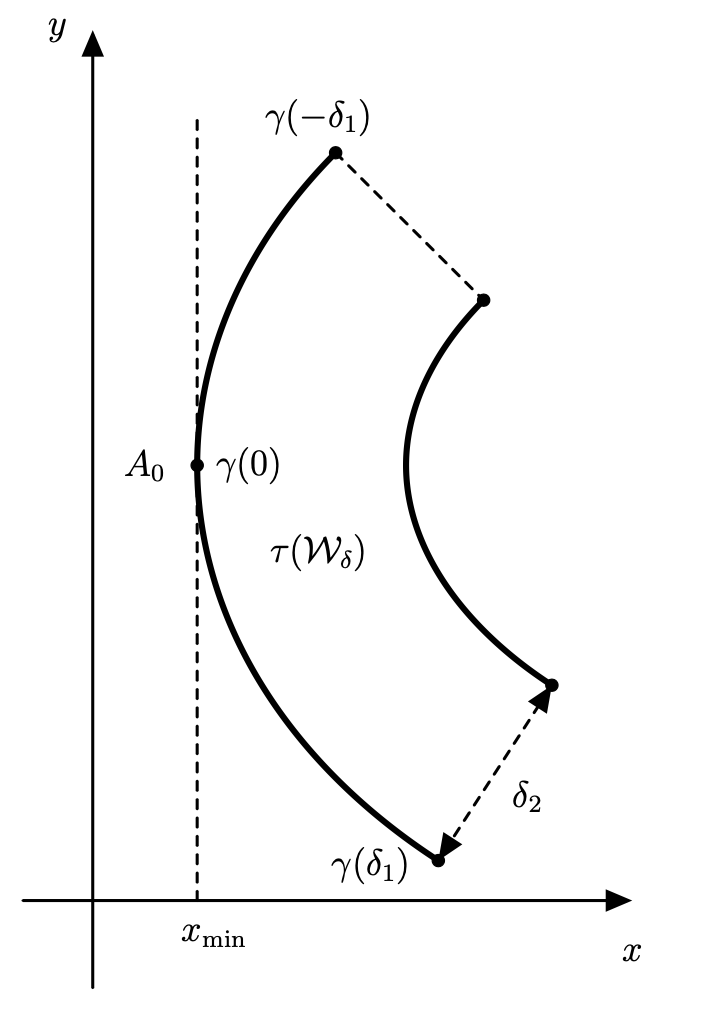
Figure 2. The local tubular coordinates

We use tubular coordinates in a neighborhood of $A_{0}$ (see for instance [6]). Due to Assumption 1.1 there exist $\delta_{1},\delta_{2}>0$ such that (see Figure 2)

$$\mathcal{W}_{\delta}=(-\delta_{1},\delta_{1})\times(0,\delta_{2})\ni(s,t)\mapsto{\boldsymbol{\tau}}(s,t)={\boldsymbol{\gamma}}(s)-t{\boldsymbol{n}}(s)\,\in{\boldsymbol{\tau}}(\mathcal{W}_{\delta})$$

induces a diffeomorphism. Here, ${\boldsymbol{n}}$ is the outward pointing normal and ${\boldsymbol{\gamma}}$ is the natural length-parametrization of the boundary $\partial\Omega$; we set ${\boldsymbol{\gamma}}(0)=A_{0}$. Denoting by $\theta(s)$ the turning angle at the point ${\boldsymbol{\gamma}}(s)\in\partial\Omega$ we may write ${\boldsymbol{n}}(s)=(\cos\theta(s),\sin\theta(s))$, the tangent vector ${\boldsymbol{\gamma}}^{\prime}(s)=(-\sin\theta(s),\cos\theta(s))$, and the curvature $\kappa(s)=\theta^{\prime}(s)$. The Jacobian of ${\boldsymbol{\tau}}=(\tau_{1},\tau_{2})=\tau_{1}{\bf e}_{1}+\tau_{2}{\bf e}_{2}$ is given by

$$m(s,t)=1-\kappa(s)t\,.$$ (3.1)

We fix $\delta_{2}>0$ so small that the map ${\boldsymbol{\tau}}$ induces a local diffeomorphism between a rectangle and the tubular neighborhood of the boundary. In view of the definition of $A_{0}$ we have

$${\boldsymbol{n}}^{\prime}(0)\cdot{\bf e}_{1}=0\,,\quad{\boldsymbol{\gamma}}^{\prime}(0)\cdot{\bf e}_{1}=0\,,\quad{\boldsymbol{\gamma}}^{\prime\prime}(0)=-\kappa_{0}{\boldsymbol{n}}(0)=\kappa_{0}{\bf e}_{1}\,,$$ (3.2)

where $\kappa_{0}=\kappa(0)$.

3.2. Spectral reduction to a localized operator

For $0<\delta\leq\delta_{1},\delta_{2}$ we define $\mathscr{L}_{h,\delta}$ to be the Dirichlet realization of $-h^{2}\partial^{2}_{x}-h^{2}\partial^{2}_{y}+x$ on $L^{2}({\boldsymbol{\tau}}(\mathcal{W}_{\delta}))$ with $\mathcal{W}_{\delta}=(-\delta,\delta)\times(0,\delta)$.

We denote by $\lambda_{n}(h,\delta)$ the corresponding eigenvalues of $\mathscr{L}_{h,\delta}$. By using the decay estimates of Theorem 2.1, we get the following:

Proposition 3.1.

For every fixed $n\geq 1$ there exist $k,K>0$ such that

$$\lambda_{n}(h,\delta)-Ke^{-k/h}\leq\lambda_{n}(h)\leq\lambda_{n}(h,\delta)\,.$$

Proof.

The second inequality is a direct consequence of the min-max variational principle since the form domain of $\mathscr{L}_{h,\delta}$ is included in the one of $\mathscr{L}_{h}$.

We now prove the first inequality but only for $n=1$. Let $\psi_{1}$ be a unit eigenvector of $\mathscr{L}_{h}$ corresponding to its groundstate $\lambda_{1}(h)$. Let $0\leq\chi_{\delta}\leq 1$ be a smooth cut-off function such that $\chi_{\delta}({\boldsymbol{\tau}}(s,t))=1$ if $|s|,t\leq\delta/2$, and $\chi_{\delta}({\boldsymbol{\tau}}(s,t))=0$ if $|s|\geq\frac{3}{4}\delta$ or $t\geq\frac{3}{4}\delta$. Then $\chi_{\delta}\psi_{1}$ belongs to the domain of $\mathscr{L}_{h,\delta}$ and since the support of the derivatives of $\chi_{\delta}$ is away from $A_{0}$, from Corollary 2.2 we have

$$\|\chi_{\delta}\psi_{1}\|=1+\mathscr{O}(e^{-k/h}),\;\|(\nabla\chi_{\delta})\nabla\psi_{1}\|=\mathscr{O}(e^{-k/h}),\;\|(\mathscr{L}_{h,\delta}-\lambda_{1}(h))\chi_{\delta}\psi_{1}\|=\mathscr{O}(e^{-k/h}).$$

Then the min-max principle implies:

$$\lambda_{1}(h,\delta)\leq\frac{\langle\chi_{\delta}\psi_{1},\mathscr{L}_{h,\delta}\chi_{\delta}\psi_{1}\rangle}{\|\chi_{\delta}\psi_{1}\|^{2}}\leq\lambda_{1}(h)+\mathscr{O}(e^{-k/h}).$$

If $n>1$, one can construct $n$ quasi-modes for $\mathscr{L}_{h,\delta}$ out of the first $n$ eigenmodes of $\mathscr{L}_{h}$ by using a similar argument. ∎

Therefore, we can focus on the spectral analysis of $\mathscr{L}_{h,\delta}$. The operator $\mathscr{L}_{h,\delta}$ is unitarily equivalent to the Dirichlet realization of

$$\mathscr{M}_{h}=-h^{2}m^{-1}\partial_{s}m^{-1}\partial_{s}-h^{2}m^{-1}\partial_{t}m\partial_{t}+\tau_{1}(s,t)\,,$$

acting on $L^{2}(\mathcal{W}_{\delta},m(s,t)\mathrm{d}s\mathrm{d}t)$.

By Taylor expansion near $(0,0)$, we have

$${\boldsymbol{\tau}}(s,t)={\boldsymbol{\gamma}}(0)+s{\boldsymbol{\gamma}}^{\prime}(0)+\frac{s^{2}}{2}{\boldsymbol{\gamma}}^{\prime\prime}(0)-t({\boldsymbol{n}}(0)+s{\boldsymbol{n}}^{\prime}(0))+\mathscr{O}(|s|^{3}+|ts^{2}|)$$

Thus, in view of (3.2), we have in particular that

$$\tau_{1}(s,t)=x_{\min}+\frac{\kappa_{0}}{2}s^{2}+t+\mathscr{O}(|s|^{3}+|ts^{2}|)\,.$$ (3.3)

Note that for $\delta$ small enough, there exists $\alpha>0$ such that for all $(s,t)\in(-\delta,\delta)\times(0,\delta)$:

$$\tau_{1}(s,t)\geq x_{\min}+\alpha(s^{2}+t)\,.$$

Proposition 3.2.

Let $M>0$. There exist $\varepsilon,C,h_{0}>0$ such that, for all $h\in(0,h_{0})$, and for all eigenfunctions $\psi$ corresponding to eigenvalues $\lambda$ of $\mathscr{M}_{h}$ with $\lambda\leq x_{\min}+Mh^{\frac{2}{3}}$, we have:

$$\int_{\mathcal{W}_{\delta}}e^{\varepsilon t^{\frac{3}{2}}/h}|\psi|^{2}\mathrm{d}s\mathrm{d}t\leq C\|\psi\|^{2}\,,$$ (3.4)

$$\int_{\mathcal{W}_{\delta}}e^{\varepsilon t^{\frac{3}{2}}/h}|h\nabla_{s,t}\psi|^{2}\mathrm{d}s\mathrm{d}t\leq Ch^{2/3}\|\psi\|^{2}\,.$$ (3.5)

Proof.

If $\delta$ is small enough then $m(s,t)\sim 1$ and $x-x_{\rm min}\sim t$. Therefore we can directly use the strategy of Proposition 2.1 applied for the eigenfunctions of $\mathscr{L}_{h,\delta}$, but in both (3.4) and (3.5) we need to choose an $\varepsilon$ which is smaller than the one in Proposition 2.1 in order to control the linear growth in $t$ of $m(s,t)-1$ and $\partial_{s}m(s,t)$. ∎

Therefore, the operator $\mathscr{M}_{h}$ can be replaced by

$$\widetilde{\mathscr{M}}_{h}=-h^{2}m^{-1}\partial_{s}m^{-1}\partial_{s}-h^{2}m^{-1}\partial_{t}m\partial_{t}+\tau_{1}(s,t)\,,$$

with Dirichlet boundary conditions, acting on $L^{2}(\mathcal{W}_{\delta,h},m(s,t)\mathrm{d}s\mathrm{d}t)$, with

$$\mathcal{W}_{\delta,h}=(-\delta,\delta)\times(0,h^{\frac{2}{3}-\eta})\,,$$

for some $\eta\in\left(0,\frac{1}{3}\right)$ with corresponding quadratic form

$$\langle\psi,\widetilde{\mathscr{M}}_{h}\psi\rangle=\int_{\mathcal{W}_{\delta,h}}\Big{(}m^{-2}|h\partial_{s}\psi|^{2}+|h\partial_{t}\psi|^{2}+\tau_{1}(s,t)|\psi|^{2}\Big{)}m\mathrm{d}s\mathrm{d}t\,.$$ (3.6)

Let $\mu_{n}(h)$ be the asociated (ordered) eigenvalues of $\widetilde{\mathscr{M}}_{h}$. The decay estimates of Proposition 3.2 are still satisfied by the eigenfunctions of $\widetilde{\mathscr{M}}_{h}$ with eigenvalues $\lambda\leq x_{\min}+Mh^{\frac{2}{3}}$. By using this exponential decay, there exist $C,h_{0}>0$ such that, for all $h\in(0,h_{0})$,

$$\mu_{n}(h)-\tfrac{1}{C}e^{-Ch^{-3\eta/2}}\leq\lambda_{n}(h,\delta)\leq\mu_{n}(h)\,.$$ (3.7)

Thus, modulo an exponentially small error, the asymptotic analysis of $\lambda_{n}(h)$ is reduced to that of $\mu_{n}(h)$.

By shrinking the spectral window, we can even get a localization with respect to the $s$ variable, as stated in the next proposition.

Proposition 3.3.

Let $M>0$ and $\eta\in(0,\frac{1}{3})$. There exist $\varepsilon,C,h_{0}>0$ such that, for all $h\in(0,h_{0})$, and for all eigenfunctions $\psi$ of $\widetilde{\mathscr{M}}_{h}$ corresponding to eigenvalues $\lambda\leq x_{\min}+h^{\frac{2}{3}}z_{1}+Mh$ we have:

$$\int_{\mathcal{W}_{\delta,h}}e^{\varepsilon s^{2}/h}|\psi|^{2}\mathrm{d}s\mathrm{d}t\leq C\|\psi\|^{2}\,.$$

Proof.

The proof follows the same lines as that of Proposition 2.1. We let $\Phi(s)=\varepsilon s^{2}/2$ and write the Agmon formula:

$$\int_{\mathcal{W}_{\delta,h}}\Big{(}m^{-2}|h\partial_{s}e^{\Phi/h}\psi|^{2}+|h\partial_{t}e^{\Phi/{h}}\psi|^{2}+{\tau_{1}}(s,t)|e^{\Phi/h}\psi|^{2}\\ -(\lambda+|\nabla\Phi|^{2})|e^{\Phi/h}\psi|^{2}\Big{)}m\mathrm{d}s\mathrm{d}t=0\,.$$

First, we drop the tangential derivative:

$$\int_{\mathcal{W}_{\delta,h}}\left(|h\partial_{t}e^{\Phi/{h}}\psi|^{2}+{\tau_{1}}(s,t)|e^{\Phi/h}\psi|^{2}-(\lambda+|\nabla\Phi|^{2})|e^{\Phi/h}\psi|^{2}\right)m\mathrm{d}s\mathrm{d}t\leq 0\,.$$

We observe from (3.3) that there exist $\tilde{k}>0$ such that $\tau_{1}(s,t)\geq x_{\rm min}+t+\tilde{k}s^{2}$. Introducing the last inequality in the above integral we get:

$$\int_{\mathcal{W}_{\delta,h}}\Big{(}|h\partial_{t}e^{\Phi/h}\psi|^{2}+t|e^{\Phi/h}\psi|^{2}\Big{)}m\mathrm{d}s\mathrm{d}t\\ +\int_{\mathcal{W}_{\delta,h}}(-\lambda+x_{\min}+\tilde{k}s^{2}-|\nabla\Phi|^{2})|e^{\Phi/h}\psi|^{2}\;m\mathrm{d}s\mathrm{d}t\leq 0\,.$$

On $\mathcal{W}_{\delta,h}$, for sufficiently small $h$ , there exists $C>0$ such that $m(s,t)\geq 1-Ch^{2/3-\eta}$. By using this in the above integrals we have that

$$(1-Ch^{2/3-\eta})\int_{\mathcal{W}_{\delta,h}}\Big{(}|h\partial_{t}e^{\Phi}\psi|^{2}+t|e^{\Phi/h}\psi|^{2}\Big{)}\mathrm{d}s\mathrm{d}t\\ +\int_{\mathcal{W}_{\delta,h}}(-\lambda+x_{\min}+\tilde{k}s^{2}-|\nabla\Phi|^{2})|e^{\Phi/h}\psi|^{2}\;m\mathrm{d}s\mathrm{d}t\leq 0\,.$$

Then, with a possibly larger constant $C$ we have that

$$(1-Ch^{2/3-\eta})\int_{\mathcal{W}_{\delta,h}}\Big{(}|h\partial_{t}e^{\Phi}\psi|^{2}+t|e^{\Phi/h}\psi|^{2}-h^{\frac{2}{3}}z_{1}|e^{\Phi/h}\psi|^{2}\Big{)}\mathrm{d}s\mathrm{d}t\\ +\int_{\mathcal{W}_{\delta,h}}(-\lambda+x_{\min}+h^{\frac{2}{3}}z_{1}+\tilde{k}s^{2}-|\nabla\Phi|^{2}-Ch^{\frac{4}{3}-\eta})|e^{\Phi/h}\psi|^{2}\;m\mathrm{d}s\mathrm{d}t\leq 0\,.$$

By using the min-max principle and the Dirichlet bracketing (only with respect to $t$, $s$ being fixed), we have

$$\int_{\mathcal{W}_{\delta,h}}\Big{(}|h\partial_{t}e^{\Phi}\psi|^{2}+t|e^{\Phi/h}\psi|^{2}-h^{\frac{2}{3}}z_{1}|e^{\Phi/h}\psi|^{2}\Big{)}\mathrm{d}s\mathrm{d}t\geq 0\,.$$

Therefore,

$$\int_{\mathcal{W}_{\delta,h}}\Big{(}(-\lambda+x_{\min}+h^{\frac{2}{3}}z_{1}+\tilde{k}s^{2}-|\nabla\Phi|^{2}-Ch^{\frac{4}{3}-{\eta}})|e^{\Phi/h}\psi|^{2}\Big{)}m\mathrm{d}s\mathrm{d}t\leq 0\,,$$

so that, using the assumption on the location of $\lambda$, we obtain

$$\int_{\mathcal{W}_{\delta,h}}(-{M}h+{\tilde{k}}s^{2}-|\nabla\Phi|^{2}-Ch^{\frac{4}{3}-{\eta}})|e^{\Phi/h}\psi|^{2}\Big{)}m\mathrm{d}s\mathrm{d}t\leq 0\,.$$

Now if $\eta\in\left(0,\frac{1}{3}\right)$ is kept fixed and $h$ is small enough, then:

$$\int_{\mathcal{W}_{\delta,h}}(\tilde{k}s^{2}-|\nabla\Phi|^{2}-{2Mh})|e^{\Phi/h}\psi|^{2}m\mathrm{d}s\mathrm{d}t\leq 0\,,$$

and

$$\int_{\mathcal{W}_{\delta,h}}\Big{(}(\tilde{k}-\varepsilon^{2})s^{2}-2Mh\Big{)}|e^{\Phi/h}\psi|^{2}\mathrm{d}s\mathrm{d}t\leq 0\,.$$

For $\varepsilon$ small enough, the conclusion follows as in the proof of Proposition 2.1. ∎

This shows that the eigenfunctions of “low energy” are localized near $A_{0}$ at a scale $h^{1/2}$ in the $s$ direction, and at a scale $h^{2/3}$ in the $t$ direction.

4. Proof of the main theorem

In view of Equation (3.7) and Proposition 3.1 our main result Theorem 1.2 is a direct consequence of the next proposition that provides the asymptotic behavior of the low-lying eigenvalues, $\mu_{n}(h)$, of the operator $\widetilde{\mathscr{M}}_{h}$ defined in the previous section.

Proposition 4.1.

Let $n\in\{1,2,\dots\}$. Then, as $h\to 0$ we have

$$\mu_{n}(h)=x_{\min}+z_{1}h^{\frac{2}{3}}+h(2n-1)\sqrt{\frac{\kappa_{0}}{2}}+\mathscr{O}(h^{\frac{4}{3}})\,.$$

In the remainder of this section we show the above proposition by obtaining suitable upper and lower bounds.

4.1. Upper bound

To get the upper bound in Theorem 1.2, it is sufficient to use convenient test functions in the domain of $\widetilde{\mathscr{M}}_{h}$ and apply the min-max principle.

Consider a smooth function $\chi$ with compact support equal to $1$ near $(0,0)$ on a scale of order $h^{1/2-\theta}$ in the $s$ direction, and on a scale of order $h^{2/3-\theta}$ in the $t$ direction, for some $\theta\in(0,\eta)$. Let us introduce the following family of test functions

$$\varphi_{n,h}(s,t)=\chi(s,t)f_{n,h}(s)a_{h}(t)\,,$$

where

1. $f_{n,h}(s)=h^{-\frac{1}{4}}f_{n}(h^{-\frac{1}{2}}s)$ and $(f_{n})_{n\in\mathbb{N}\setminus\{0\}}$ is an $L^{2}(\mathbb{R})$-normalized family of eigenfunctions of the harmonic oscillator $-{h^{2}}\partial^{2}_{s}+\frac{\kappa_{0}}{2}s^{2}$ (rescaled Hermite functions),

2. $a_{h}(t)=h^{-\frac{1}{3}}\mathrm{Ai}(h^{-\frac{2}{3}}t-z_{1})$ where $\mathrm{Ai}$ is the $L^{2}(\mathbb{R}^{+})$ normalized Airy function and $-z_{1}<0$ is its first zero. In particular, we have that $a_{h}(t)$ satisfies

   $$(-h^{2}\partial_{t}^{2}+t)a_{h}(t)=z_{1}h^{2/3}a_{h}(t)$$

   for $t>0$ with Dirichlet boundary conditions.

An explicit computation shows that for any $n\in\mathbb{N}$ there exist constants $\varepsilon,c>0$ such that

$$\int_{\mathbb{R}}e^{\varepsilon s^{2}/h}|f_{n,h}(s)|^{2}\mathrm{d}s\leq c\,,\quad\int_{\mathbb{R}^{+}}e^{\varepsilon t^{\frac{3}{2}}/h}|a_{h}(t)|^{2}\mathrm{d}t\leq c\,.$$ (4.1)

Using this we immediately see that we find $c_{1},c_{2}>0$ such that

$$1\geq\|\varphi_{n,h}\|^{2}\geq 1-c_{1}\int t\left|\varphi_{n,h}(s,t)\right|^{2}\mathrm{d}s\mathrm{d}t\geq 1-c_{2}h^{2/3}.$$ (4.2)

We are interested in estimating the matrix elements $\langle\varphi_{n^{\prime},h},(\widetilde{\mathscr{M}}_{h}-x_{\rm min})\varphi_{n,h}\rangle.$ First, we notice that the support of $\chi-1$ and the supports of the derivatives of $\chi$ are located in a region where either $h^{-1/2}|s|\geq Ch^{-\theta}$ or $h^{-2/3}t\geq Ch^{-\theta}$, thus all the integrals entering the matrix element which contain such derivatives will be of order $h^{-\infty}$ due to the exponential localization of the $f_{n}$’s and of ${\rm Ai}$. Second, the operators $h\partial_{s}$ and $h\partial_{t}$ acting on $f_{n,h}$’s and $a_{h}$ respectively will generate a factor of at most $h^{1/3}$, and each integral contains two such factors; thus each term in the scalar product has an order of magnitude of at most $h^{2/3}$. Third, if we replace the function $m$ in (3.1) by $1$, the error contains an extra factor $t$ which due to the decay of $a_{h}$ may be replaced by $h^{2/3}$. Together with the a-priori decay of $h^{2/3}$ coming from the derivatives, this error term will grow at most like $h^{4/3}$.

Moreover, replacing $\tau_{1}(s,t)-x_{\rm min}$ with $\frac{\kappa_{0}}{2}s^{2}+t$ will produce an error like $h^{3/2}$. Thus we may write:

$$\langle\varphi_{n^{\prime},h},(\widetilde{\mathscr{M}}_{h}-x_{\rm min})\varphi_{n,h}\rangle= h^{2}\int_{\mathbb{R}}\left(\partial_{s}f_{n,h}\overline{\partial_{s}f_{n^{\prime},h}}+\frac{\kappa_{0}}{2}s^{2}f_{n,h}\overline{f_{n^{\prime},h}}\right)\mathrm{d}s$$

$$+\delta_{n,n^{\prime}}\int_{\mathbb{R}_{+}}\left(|\partial_{t}a_{h}|^{2}+t|a_{h}|^{2}\right)\mathrm{d}t+\mathscr{O}(h^{4/3})$$

$$= \delta_{n,n^{\prime}}\left((2n-1)h\sqrt{\frac{\kappa_{0}}{2}}+z_{1}h^{2/3}\right)+\mathscr{O}(h^{4/3}).$$ (4.3)

Using similar arguments, the Gram-Schmidt matrix elements $\langle\varphi_{n^{\prime},h},\varphi_{n,h}\rangle$ will equal $\delta_{n,n^{\prime}}+\mathscr{O}(h^{2/3})$. Thus if $N$ is fixed and $h$ is small enough, the subspace

$$\underset{1\leq j\leq N}{\text{span}}\varphi_{j,h}$$

will have dimension $N$ and we may find an orthonormal basis $\{\psi_{n,h}\}_{n=1}^{N}$ such that

$$\psi_{n,h}=\sum_{j=1}^{N}c_{j}\varphi_{j,h},\quad c_{j}=\delta_{n,j}+\mathscr{O}(h^{2/3})\,.$$

Thus the matrix elements $\langle\psi_{n^{\prime},h},(\widetilde{\mathscr{M}}_{h}-x_{\rm min})\psi_{n,h}\rangle$ will obey the same estimate as in (4.1), which via the min-max principle imply

$$\mu_{n}(h)\leq x_{\min}+z_{1}h^{\frac{2}{3}}+h(2n-1)\sqrt{\frac{\kappa_{0}}{2}}+\mathscr{O}(h^{\frac{4}{3}}),\quad 1\leq n\leq N.$$

4.2. Lower bound

Let $N\geq 1$ and consider a family of eigenfunctions $(\psi_{j,h})_{1\leq j\leq N}$ associated with the eigenvalues $(\mu_{j}(h))_{1\leq j\leq N}$. We let

$$\mathscr{E}_{N}(h)=\underset{1\leq j\leq N}{\mathrm{span}}\,\psi_{j,h}\,\subset L^{2}(\mathcal{W}_{\delta,h},m\mathrm{d}s\mathrm{d}t)\,.$$

Note that the decay estimates of Propositions 3.2 and 3.3 can be extended to $\psi\in\mathscr{E}_{N}(h)$.

Let us choose any $\psi\in\mathscr{E}_{N}(h)$ with norm one. Because $m(s,t)\leq 1$, we have the important inequality

$$1=\int_{\mathcal{W}_{\delta,h}}|\psi|^{2}m\mathrm{d}s\mathrm{d}t\leq\|\psi\|^{2}_{L^{2}(\mathcal{W}_{\delta,h};\mathrm{d}s\mathrm{d}t)}\,.$$ (4.4)

We also have

$$\mu_{N}(h)\geq\langle\widetilde{\mathscr{M}}_{h}\psi,\psi\rangle=\int_{\mathcal{W}_{\delta,h}}\left(m|h\partial_{t}\psi|^{2}+m^{-1}|h\partial_{s}\psi|^{2}+m{\tau}_{1}(s,t)|\psi|^{2}\right)\mathrm{d}s\mathrm{d}t\,.$$ (4.5)

We recall that $m(s,t)=1-\kappa(s)t$ so that, using (3.5) in the second inequality below,

$$\begin{split}\langle{\widetilde{\mathscr{M}}_{h}}\psi,\psi\rangle&\geq\int_{\mathcal{W}_{\delta,h}}\left(|h\partial_{t}\psi|^{2}+|h\partial_{s}\psi|^{2}+m{\tau}_{1}(s,t)|\psi|^{2}\right)\mathrm{d}s\mathrm{d}t-C\int_{\mathcal{W}_{\delta,h}}t|h\nabla_{s,t}\psi|^{2}\mathrm{d}s\mathrm{d}t\\ &\geq\int_{\mathcal{W}_{\delta,h}}\left(|h\partial_{t}\psi|^{2}+|h\partial_{s}\psi|^{2}+m{\tau}_{1}(s,t)|\psi|^{2}\right)\mathrm{d}s\mathrm{d}t-Ch^{4/3}\,,\\ &=x_{\rm min}+\int_{\mathcal{W}_{\delta,h}}\left(|h\partial_{t}\psi|^{2}+|h\partial_{s}\psi|^{2}+m{(\tau_{1}(s,t)-x_{\rm min})}|\psi|^{2}\right)\mathrm{d}s\mathrm{d}t-Ch^{4/3}\\ &{\geq x_{\min}+\int_{\mathcal{W}_{\delta,h}}\left(|h\partial_{t}\psi|^{2}+|h\partial_{s}\psi|^{2}+\left(t+\kappa_{0}\frac{s^{2}}{2}\right)|\psi|^{2}\right)\mathrm{d}s\mathrm{d}t-Ch^{4/3}}\\ &\qquad{-\tilde{C}\int_{\mathcal{W}_{\delta,h}}(|s^{2}t|+|t^{2}|)|\psi|^{2}\mathrm{d}s\mathrm{d}t},\end{split}$$

the last integral can be estimated to be of order $h^{4/3}$ as well using the exponential decay in the $s$ and $t$ variables (Propositions 3.2 and 3.3). Then, there is a $C>0$ such that

$$\langle\widetilde{\mathscr{M}}_{h}\psi,\psi\rangle\geq x_{\min}+\int_{\mathcal{W}_{\delta,h}}\left(|h\partial_{t}\psi|^{2}+|h\partial_{s}\psi|^{2}+\left(t+\kappa_{0}\frac{s^{2}}{2}\right)|\psi|^{2}\right)\mathrm{d}s\mathrm{d}t-C{h^{4/3}}\,.$$

Now using the inequalities in (4.5) and (4.4) we have:

$$\int_{\mathcal{W}_{\delta,h}}\left(|h\partial_{t}\psi|^{2}+|h\partial_{s}\psi|^{2}+\left(t+\kappa_{0}\frac{s^{2}}{2}\right)|\psi|^{2}\right) \mathrm{d}s\mathrm{d}t\leq\mu_{N}(h)-x_{\min}+{Ch^{4/3}}$$ (4.6)

$$\leq(\mu_{N}(h)-x_{\min}+{Ch^{4/3}})\|\psi\|^{2}_{L^{2}(\mathrm{d}s\mathrm{d}t)}\,.$$

On the left hand side of the above identity we recognize the quadratic form associated to the operator

$$\mathscr{A}_{h}\otimes\mathbf{1}+\mathbf{1}\otimes\mathscr{H}_{h}\,,$$

where $\mathscr{A}_{h}=-h^{2}\partial^{2}_{t}+t$ on $L^{2}((0,+\infty),\mathrm{d}t)$ with Dirichlet boundary conditions and $\mathscr{H}_{h}=-h^{2}\partial^{2}_{s}+\kappa_{0}\frac{s^{2}}{2}$ on $L^{2}((-\infty,\infty),\mathrm{d}s)$. The spectrum of $\mathscr{A}_{h}$ and $\mathscr{H}_{h}$ is given by

$$\mathrm{sp}(\mathscr{A}_{h})=\Big{\{}z_{n}h^{2/3}\,,\,n\geq 1\Big{\}}\,,\qquad\mathrm{sp}(\mathscr{H}_{h})=\Big{\{}(2n-1)h\sqrt{\frac{\kappa_{0}}{2}}\,,\,n\geq 1\Big{\}}\,.$$

Thus, for $h$ small enough, the $N$-th eigenvalue of $\mathscr{A}_{h}\otimes\mathbf{1}+\mathbf{1}\otimes\mathscr{H}_{h}$, denoted by $\nu_{N}(h)$, is given by

$$\nu_{N}(h)=z_{1}h^{2/3}+(2N-1)h\sqrt{\frac{\kappa_{0}}{2}}\,.$$ (4.7)

Notice that the set $\mathscr{E}_{N}(h)$ is contained in the form domain of $\mathscr{A}_{h}\otimes\mathbf{1}+\mathbf{1}\otimes\mathscr{H}_{h}$ and, seen as a subset of $L^{2}(\mathcal{W}_{\delta,h};\mathrm{d}s\mathrm{d}t)$, still has the dimension $N$ for $h$ small enough. This is because the $\psi_{j,h}$’s are almost orthogonal in the “flat” space, up to an error of order $h^{2/3}$. Thus, by the min-max principle, we have

$$\nu_{N}(h)\leq\sup_{\psi\in\mathscr{E}_{N}(h)}\frac{\left\langle\Big{(}\mathscr{A}_{h}\otimes\mathbf{1}+\mathbf{1}\otimes\mathscr{H}_{h}\Big{)}\psi,\psi\right\rangle_{L^{2}(dsdt)}}{\|\psi\|^{2}_{L^{2}(\mathrm{d}s\mathrm{d}t)}}\leq(\mu_{N}(h)-x_{\min}+{Ch^{4/3}})\,,$$ (4.8)

where in the last inequality we used (4.6). This implies the desired lower bound and concludes the proof of Proposition 4.1.

Acknowledgment

D.K. has been supported by the EXPRO grant No. 20-17749X of the Czech Science Foundation (GACR). D.K. is also grateful to the Aalborg University for supporting his stay in 2019. E.S. has been partially funded by Fondecyt (Chile) project # 118–0355 and thanks Esteban Ramos Moore for stimulating discussions. H.C., E.S, and N.R. are deeply grateful to the Mittag-Leffler Institute where this collaboration was stimulated during the thematic semester “Spectral Methods in Mathematical Physics” in 2019. E.S. and N.R. are also grateful to the CIRM where the ideas of this paper were discussed (“Research in Pairs” session in 2019).

References

• [1] Y. Almog. The stability of the normal state of superconductors in the presence of electric currents. SIAM J. Math. Anal., 40:824–850, 2008.
• [2] Y. Almog, D. S. Grebenkov, and B. Helffer. Spectral semi-classical analysis of a complex Schrödinger operator in exterior domains. J. Math. Phys., 59(4):041501, 12, 2018.
• [3] Y. Almog, D. S. Grebenkov, and B. Helffer. On a Schrödinger operator with a purely imaginary potential in the semiclassical limit. Comm. Partial Differential Equations, 44(12):1542–1604, 2019.
• [4] Y. Almog and R. Henry. Spectral analysis of a complex Schrödinger operator in the semiclassical limit. SIAM J. Math. Anal., 48:2962–2993, 2016.
• [5] G. Bastard, E. E. Mendez, L. L. Chang, and L. Esaki. Variational calculations on a quantum well in an electric field. Phys. Rev. B, 28:3241–3245, Sep 1983.
• [6] S. Fournais and B. Helffer. Spectral methods in surface superconductivity, volume 77 of Progress in Nonlinear Differential Equations and their Applications. Birkhäuser Boston, Inc., Boston, MA, 2010.
• [7] D. Grebenkov, B. Helffer, and R. Henry. The complex Airy operator on the line with a semipermeable barrier. SIAM J. Math. Anal., 49:1844–1894, 2017.
• [8] D. S. Grebenkov and B. Helffer. On spectral properties of the Bloch-Torrey operator in two dimensions. SIAM J. Math. Anal., 50(1):622–676, 2018.
• [9] P. Harrison and A. Valavanis. Quantum wells, wires and dots: theoretical and computational physics of semiconductor nanostructures. John Wiley & Sons, 2016.
• [10] V. Harutyunyan. Cylindrical nanolayer in the strong uniform electrical field: The field localization of carriers and electrooptical transitions. Physica E, 41(4):695 – 700, 2009.
• [11] B. Helffer, A. Kachmar, and N. Raymond. Tunneling for the Robin Laplacian in smooth planar domains. Commun. Contemp. Math., 19(1):1650030, 38, 2017.
• [12] R. Henry. On the semi-classical analysis of Schrödinger operators with purely imaginary electric potentials in a bounded domain. arXiv:1405.6183, 2014.
• [13] P. Keraval. Formules de Weyl par réduction de dimension. Applications à des Laplaciens électro-magnétiques. PhD thesis, Université de Rennes 1, 2018.
• [14] J. Lee and H. N. Spector. Stark effect in the optical absorption in quantum wires. Journal of Applied Physics, 97(4):043511, 2005.
• [15] A. Martinez. A general effective Hamiltonian method. Atti Accad. Naz. Lincei Rend. Lincei Mat. Appl., 18(3):269–277, 2007.
• [16] D. Miller, D. Chemla, T. C. Damen, T. Wood, C. Burrus, A. Gossard, and W. Wiegmann. Band-edge electroabsorption in quantum well structures: The quantum-confined Stark effect. Physical Review Letters, 53:2173–2176, 1984.
• [17] D. A. B. Miller, D. S. Chemla, and S. Schmitt-Rink. Electroabsorption of highly confined systems: Theory of the quantum-confined Franz–Keldysh effect in semiconductor quantum wires and dots. Applied Physics Letters, 52(25):2154–2156, 1988.
• [18] T. G. Pedersen. Stark effect in finite-barrier quantum wells, wires, and dots. New Journal of Physics, 19(4):043011, apr 2017.
• [19] T. G. Pedersen. Stark effect in spherical quantum dots. Phys. Rev. A, 99:063410, Jun 2019.
• [20] N. Raymond. Bound states of the magnetic Schrödinger operator, volume 27 of EMS Tracts in Mathematics. European Mathematical Society (EMS), Zürich, 2017.
• [21] B. Sukumar and K. Navaneethakrishnan. Polarizability of a carrier in an isolated well of a quantum-well wire. Phys. Rev. B, 41:12911–12914, Jun 1990.
• [22] G. J. Vázquez, M. del Castillo-Mussot, and H. N. Spector. Transverse Stark effect of electrons in a semiconducting quantum wire. Physica Status Solidi (B), 240(3):561–564, 2003.
• [23] S. Wang, Y. Kang, and C. Han. Transverse Stark effect in the optical absorption in a square semiconducting quantum wire. Journal of Semiconductors, 34(10):102001, oct 2013.
• [24] G. Wei, S. Wang, and G. Yi. Stark effect of electrons in semiconducting rectangular quantum boxes. Microelectronics Journal, 39(5):786 – 791, 2008.
• [25] G. Yi, G. Wei, and H. Wu. Transverse Stark effect in a rectangular semiconducting quantum wire. Physica Status Solidi (b), 244(12):4651–4659, 2007.