Multi-agent navigation based on deep reinforcement learning and traditional pathfinding algorithm

Abstract

We develop a new framework for multi-agent collision avoidance problem. The framework combined traditional pathfinding algorithm and reinforcement learning. In our approach, the agents learn whether to be navigated or to take simple actions to avoid their partners via a deep neural network trained by reinforcement learning at each time step. This framework makes it possible for agents to arrive terminal points in abstract new scenarios.

In our experiments, we use Unity3D and Tensorflow to build the model and environment for our scenarios. We analyze the results and modify the parameters to approach a well-behaved strategy for our agents. Our strategy could be attached in different environments under different cases, especially when the scale is large.

Key words: Collision Avoidance Problem, Multi-agent Problem, Deep Reinforcement Learning

1 Introduction

Multi-agent navigation problem (also known as multi-agent pathfinding and collision avoidance problem) has been a highly-concerned topic in control, robotics and optimization. The research of this problem has great potential in engineering applications. One of the major directions is to develop reliable and high efficient navigating algorithm (or strategy) for agents to arrive their terminal points without any collisions.
In general, a pathfinding and collision avoiding mission requires the agent(s) to figure out collision-free optimized paths $\gamma$ from the set-off(s) to the target(s). We can define such a problem rigorously as the following:
Let $p$ be an agent, $\alpha$ its set-off, $\beta$ its target and $S\subset\mathbb{R}^{2}$ its motion space with an obstacle set $\mathcal{B}=\{B_{k}|B_{k}\subset\mathbb{R}^{2},\partial{B_{k}}\subset C(\mathbb{R}^{2})\}$, where $\partial{B_{k}}$ means the boundary of $B_{k}$. These boundaries $\partial{B_{k}}$ can be regarded as closed, continuous loops on Euclidean plane $\mathbb{R}^{2}$. In our work, we further suppose that $\partial{B_{k}}$ are (piecewise) smooth.
Suppose the position and velocity of $p$ at time step $t$ are $\gamma(t)=(x(t),y(t))$, $\textbf{v}(t)=\dot{\gamma}(x)=(\dot{x}(t),\dot{y}(t))=(u(t),w(t))$, respectively, and the maximum time T, the optimization goal of the problem is:

$$\min_{\gamma}{\int_{0}^{T}{|\textbf{v}}_{i}(t)|dt}$$ (1)

subject to ${\gamma}_{i}(t)\not\in S/\cup_{B_{k}\in\mathcal{B}}B_{k}$, $|{\gamma}_{i}(t)-\ {\gamma}_{j}(t)|\geq d_{safe},$ $\gamma(0)=s,$ $\gamma(T)=t,\ t\in[0,T]$. Here $\gamma(t)=({\gamma}_{1}(t),{\gamma}_{2}(t))$is the path, which is second-order differentiable with respect to $t$.
Two classes of methods have been developed to solve this problem for the single-agent case. The first class is usually referred to as continuous methods that employ calculus of variation [1]. In those works, the problem is described as an optimal control problem with constraints: given the set of obstacles $\{B_{k}\}$, the optimization target of some agent $a$ is to minimize the following functional along its path $\gamma$:

$$J(\gamma)=\int_{0}^{T}L(t,\gamma(t),\dot{\gamma}(t))dt\$$ (2)

subject to $d({a,\partial B}_{k})>d_{safe}$. Here $L(t,\gamma(t),\dot{\gamma}(t))$ is an energy functional of the time $t$, the position $\gamma(t)$ and the velocity $\dot{\gamma}(t)$, usually defined by specified circumstances; $d_{safe}$ is the minimized distance from the $a$ to the bound of $P_{k}$, and $d_{safe}$, the "safe distance" between $p$ and any obstacles [1].
Discretized methods, on the other hand, are also well developed. In early works, researchers discretize the environment of agent(s) into some grid world or graph and develop efficient algorithms to figure out global optimal solution for the agent which is allowed to take several discrete actions. Typical discretize algorithm include $A*$ search algorithm [2] and Dijkstra‘s algorithm [3]. This line of thinking is still efficacious in many fields including engineering, robotics and commercial games, yet it does not work well in complicated cases, such as that with a stochastic environment or large scale. Several methods have been developed to solve this problem. One method related to our work is to use triangular mesh [4] instead of grid world to decrease the computational cost [5]. Compared to continuous methods, discretized methods typically require smaller computational cost and have higher efficiency.
Multi-agent navigation [6],[7], [8], however, arouses new challenges for us. First of all, in such a system, each agent has to be considered with a group of independent constraints, which brings large cost for numerical calculation whether we adopt continuous or discontinuous methods. Secondly, the model of the problem is NP-hard and the scale of the problem in practice can usually grow extremely large. In practice, every agent need to avoid not only static obstacles but also their partners who themselves are also dynamical. Getting precise solutions numerically via traditional tools is thus expensive and time-costing.
Fortunately, some characteristics of the problem offer researchers new implication. The Markov property of the process of navigation implies the possibility of using reinforcement learning tools. For each agent, the state of t $s_{t}$ is completely determined by $s_{t-1}$ and its decision (or action) at $t-1$, $a_{t-1}$.

$$s_{0}\stackrel{{\scriptstyle a_{0}}}{{\rightarrow}}s_{1}\stackrel{{\scriptstyle a_{1}}}{{\rightarrow}}…\stackrel{{\scriptstyle a_{t-1}}}{{\rightarrow}}s_{t}$$

Reinforcement Learning (RL) has immense advantage in dealing with robot navigation problem. The advantage of reinforcement learning is that we do not have to precisely "know" exactly the model of the problem; instead, the algorithm itself could figure it out. Decisions of agents are completely obtained by a parameterized policy which can be optimized (trained) based on training data of the systems. Such path thus circumvent the challenge of defining and verifying a complicated model represented by some group of equations that are usually hard to solve.
In [9], the author introduces an example in which the agent (a Khepera robot) is required to explore the environment and avoid collision with obstacles as long as possible. The problem is finally solved by mean-square policy iteration algorithm, where the task of the agent is specified by a reward function. In the training process, the agent gathers local information of the environment via 8 distance sensors, and its navigation strategy, also known as behavioral policy in reinforcement learning, is trained by a self-organizing map [10].
Reinforcement learning has also shown its power in solving multi-robot navigation problems. Some recent works develop high performance navigating policy for agents via evolutionary reinforcement learning [11] and deep reinforcement learning [12]-[13], where decentralized and non-communicative method is used to train their agents. agents gain local information of the environment and make their decision independently while updating the same policy. In [12], researchers study a small scale decentralized multi-agent collision avoidance problem. In that work a bilateral (two-agent) value function is defined based on the state of a certain agent and its neighbor. However, agents in this work are supposed to be omniscient to their surroundings, which is impossible in real world. As a progress, [13] further studies the problem in a larger scale, and develops a decentralized framework, in which the model of the agents is based on a real product. In the training, a group of 20 agents detects surrounding environment through a series of distance sensors and share the common policy. In their tests, agents are able to finish tasks in many rich and complex scenarios.
Both of these works employ a class of deep reinforcement learning algorithm known as policy gradient methods (or gradient-based methods) [14], [15]. Instead of estimating value function, this class of algorithms directly searches for the optimal parameter set in the parameter set of the policy, allowing researchers to solve problems with continuous state and action space and large-scale inputs.
There are still some problems remained for us. First of all, deep reinforcement learning merely guarantees collision-free paths, but not the shortest ones–these algorithms do not consider the global structure of the maps (the activity area for the agents), which makes it fairly possible that the final path is not globally optimized. Secondly, training and testing for agents are only done in limited types of scenarios. This leads to weak robustness for variance of environments. Agents may suffer much weaker performance, i.e., getting higher collision rate or longer average path when the environment varies. For instance, a policy trained using small group of agents may not work well for larger group anymore [13], [16]. Retraining the agents for every new environment, on the other hand, can be expensive and typically require extra designing on the algorithm [17].
The advantages of reinforcement learning and traditional pathfinding methods inspire us to combine them together—pathfinding problem has been efficaciously solved by traditional methods, and collision avoidance by reinforcement learning.
In this work, we explore the direction on combining traditional algorithms and machine learning methods. We propose a framework that merge multi-agent reinforcement learning and classical pathfinding algorithm together. In our framework, the local decision policy on pathfinding and collision avoidance is parameterized and optimized via reinforcement learning using a policy-gradient algorithm[14], while the decisions of agents include an action that obtained by a determined and global pathfinding algorithm [2]. The complete logic of our framework is shown in (Figure 1). Our numerical results show that this framework achieve the following advantages: (1) Strong robustness to variance of environment, including different maps, random starting and terminus points and different density of agents; (2) Higher efficiency of navigation compared to pure learning method [13] on the same path-programming problems; (3) Flexibility. This means that the policy trained from a fundamental scenario can be used in other scenarios without losing too much accuracy; (4) Independent decision. Unlike some previous work using complete centralized framework [23], while still adopting a centralized training process, our work enables for each agent a decentralized decision process.

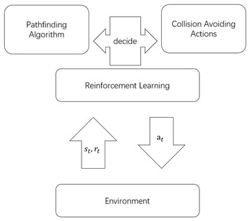
Figure 1: An Overview of Our Approach

This paper is organized as follows. In section 2 we introduce some related works in multi-agent reinforcement learning. The model of multi-agent navigation problem and our approach are presented in section 3. The results and the main results of simulations are reported in section 4, and our works are discussed and a conclusion is made in section 5.

2 Related Work

Multi-agent navigation problem has gained a large fragment of attention from researchers, Multi-agent navigation [6],[7], [8]. Several directions have been explored and many approaches have been developed to attack this problem, including classical algorithm in computer science [6], constraint optimization [7] and conflict based searching [8], [18].
There has also been increasing focus on solving multi-agent navigation problem using machine learning and reinforcement learning. The main inspiration of researchers is usually to make the decision policy highly adaptive to unknown or stochastic environments. Some latest progresses have been made via evolutionary artificial neural networks (ANN) [19] or reinforcement learning implemented by evolutionary neural networks [11]. Other works usually aim at coping with very large scale problems in which agents can only gather partial and local information of environment. For instance, in [20], a deep neural work architecture is adopted to cope with the swarm coordinate problem in which agents could only get information from nearby partners. Another related work is [21] in which deep reinforcement learning algorithm is used to build a mapless navigator for agents based on locally visual sensors.
Multi-agent reinforcement learning (MARL) has gained great interest from researchers in applied math and computer science. The improvement and comparison in our work are based on a recent study about MARL on $\mathbb{R}^{2}$ [13], where a policy-gradient method is adopted and several complex scenarios are tested.
One of the most important directions that related to our study stands on how to enhance the performance of learning algorithms via attaching the learning algorithm with extra approaches or tools. For instance, imitation learning–introducing expert knowledge to the model [22] can improve the robustness of learning and make the agents adaptive to different environments. In another example [23], randomized decision process is introduced into the framework to decrease the conflicts among agents and improve synergies of the whole system.
Some prior works also focus on solving practical problems via combining MARL with other fields of knowledge. For example, in [18], MARL is combined with conflict based search, enabling the agents to cope with pathfinding problems with sequential subtasks. In another work [24], Mattia and his group use one-step Q-learning algorithm and wavelet adopted vortex method to build the dynamical model for schools of swimming fish.
Merging RL or MARL with other fields of methods is also a direction gaining increasing attention. For instance, Hu proposes the Nash Q-learning algorithm by attaching the Lemke-Houson algorithm [25] to the iteration of policy updating to receive a Nash equilibrium for an N-agent game [26]. In another work [16], an adaptive algorithm that combines MARL and multi-agent game theory is developed to cope with MARL in highly crowded cases.

3 Approach

The main idea of our work is to combine traditional pathfinding algorithm and reinforcement learning. In other words, we employ reinforcement learning to train the collision-avoidance behavioral strategy for the agents while a pathfinding algorithm is attached to navigate the agents to their target. The agents learn to decide whether to be navigated or to avoid their partners at each time step. Every agent in the scenario acts independently, while training is centralized (Figure 2) – all the agents share the same strategy ${\pi}_{\theta}$ and parameter set $\theta$.

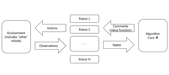
Figure 2: Reinforcement Learning

We begin this section with introducing the model of the problem; then we introduce the framework of our approach, including the state, action reward design and algorithm of reinforcement learning.

3.1 Notations

Before formal discussions, we introduce some basic notations in this paper.

• $\mathbb{R}^{d}$: $d$-dimensional Euclidean space;

• $C(X),C^{k}(X),C^{\infty}(X)$: continuous/$k$-degree differentiable/smooth functions on space $X$ where $X$ is usually a subspace of some Euclidean space;

• $\Delta X$: the space of distributions on some space $X$;

• $\mathbb{E}V$: the expectation of some random variable $V$;

• $|v|$: norm of vector $v\in\mathbb{R}^{d}$;

• $\mathcal{S}$: state space of agents in learning;

• $\mathcal{A}$: action space of agents in learning;

3.2 The model of the problem

The model of $N$-agent navigation problem in our work is shown as the following: Let $i=1,…,N$ be the index of agents. For any agent $i$, let $\alpha_{i}$ be its starting point and $\beta_{i}$ its terminal point. All agents are running on a motion space $S=[0,l]\times[0,l]\subset\mathbb{R}^{2}$ with an obstacle set $\mathcal{B}=\{B_{k}|B_{k}\subset\mathbb{R}^{2},\partial B_{k}\subset C^{\infty}(\mathbb{R}^{2})\}$.
Suppose that each agent $i$ has a path $\gamma$ and its the position and velocity at time step $t$ is ${\gamma}_{i}(t)=(x_{i},y_{i})\in S\subset\mathbb{R}^{2}$,$\ {\textbf{v}}_{i}(t)=(u_{i},w_{i})\in\left[0,1\right]*[0,2\pi)$ respectively. Furthermore, we note the safe distance between each two agents as $d_{safe}$ and the terminal time as $T_{i}\leq T$ for each agent $i$. All these variables are listed as in Table1.

Table 1: Variables of Agent

Notation	Definition
$\gamma_{i}(t)$	Position of $i$ at $t$
$\textbf{v}_{i}(t)$	Velocity of $i$ at $t$
$T_{i}$	Terminal time of $i$
$d_{safe}$	The safe distance between agents

In addition, we assume that:

• $l\gg d_{safe}$;

• Each agent $i$ knows its corresponding $\alpha_{i},\beta_{i}$ and the structure of the map, but there is no communication among agents.

Now it is a fair point to propose the main objective of our approach.
First of all, we introduce the goal of policy, that is, the goal of optimization that the optimal policy of agents should achieve.
Let $\pi$ be any policy for agents and $\pi*$ be the optimal policy. Consider a discretized partition of the time interval $[0,T]$, $0<t_{1}<t_{2}<...<t_{final}=T$. In our work, we take $t_{a}=a\Delta t$ where $\delta t$ notes the time unit for simulation. For simplicity of notation and without loss of generality, we assume that $T>>1$ and take $\delta t=1$. Thus, we use can denote any time point by an integer $t\in\mathbb{Z}_{+}$.
As a consequence, we can represent the dynamics of the system as the following:

$$\left\{\begin{aligned} &\gamma_{i}(t+1)=\gamma_{i}(t)+v_{i}(t)\\ &\gamma_{i}(0)=\alpha_{i},\gamma_{i}(T_{i})=\beta_{i}\\ &\gamma_{i}(t)\notin S/\cup B_{k},|{\gamma}_{i}(t)-{\gamma}_{j}(t)|\geq d_{safe}\\ &i=0,1,...,N,t=0,1,...,T\end{aligned}\right.$$ (3)

In this system, the velocity $v_{i}(t)$ is chosen by some policy $\pi$ for each agent $i$ at each time step $t$.
Thus, given any set of $\alpha_{i},\beta_{i}$, at each time step $t$, a policy $\pi$ can determine a series of paths ${\gamma}_{\pi}(t;\alpha_{i},\beta_{i}),i=1,...,N$. To measure how well the policy works, we may compute the average of all the paths, that is,

$$S(\pi;\alpha_{i},\beta_{i},i=1,...,N)=\frac{1}{N}\sum_{i=1}^{N}Length({\gamma}_{\pi}(t;\alpha_{i},\beta_{i}))=\frac{1}{N}\sum_{i=1}^{N}\sum_{t=0}^{T_{i}}|v_{i}(t)|$$ (4)

In this work, we wish to optimize $\pi$, i.e., to obtain $\pi*$ among the set of all $\pi$ by apply reinforcement learning. To achieve this, we parameterize $\pi$ with a set of parameters $\theta=(\theta_{1},...,\theta_{M})\in\mathbb{R}^{M}$ where $M$ is the dimension. Then we rewrite $\pi$ as $\pi_{\theta}$.
To measure the performance of a policy $\pi_{\theta}$, we consider a dataset $\mathcal{D}$ of starting points and terminal points, i.e., $\mathcal{D}=\{(\alpha_{1}^{m},...,\alpha_{N}^{m};\beta_{1}^{m},...,\beta_{N}^{m}),m=1,...,M\}$. Then we can define a cost function $R$ of $\theta$ by computing the average of $S(\pi;\alpha_{i},\beta_{i},i=1,...,N)$ among all data in $\mathcal{D}$:

$$R(\theta;\mathcal{D})=\frac{1}{M}\sum_{m=1}^{M}S(\pi_{\theta};\alpha_{i},\beta_{i},i=1,...,N)$$ (5)

The optimum $\theta*$ is defined as:

$$\theta*=argmin_{\theta}R(\theta;\mathcal{D})$$ (6)

The goal of learning is to optimize $\theta*$ based on some dataset $\mathcal{D}$. We will discuss our learning framework in the following sections.

3.3 Multi-Agent Reinforcement Learning

In this work, we adopt a class of policy gradient method [14],[15] to train the policy $\pi_{\theta}$. This method has shown its capability on solving machine-learning problems with continuous state space in many other works ([9], [13]). We discuss it with more detail in section 3.3.6.
Agents are trained through interaction with the environment (scenarios). In the simulation, each agent learns whether to find the path to its target, or to take some simple actions to avoid approaching objects at each time step $t$. The maximum time step is $T$. The trajectory of each agent is then defined as:

$$h=\{(s_{t},a_{t})|t=1,2,…,T\}$$ (7)

In the following part of this section we omit the index i, since the definition of each agent is exactly the same. The position, velocity, starting point, terminal point of agent at time step $t$ is then noted as $\gamma(t),v(t),\alpha,\beta$. The terminal time of agent is noted as $T$.
Specific model of learning is introduced as the following.

3.3.1 State

In this work, each agent is modeled as disc with radius $r=1$ physical unit, equipped with 45 range sensors around (Figure 3). The sensors distribute uniformly around the agent, and each of them return the distance and type (that is, static or motile) of other objects. The ray distance is noted as $d$.

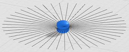
Figure 3: The model of robot

Each agent gains its state at time $t$ $s_{t}=(o_{t})$, where $o_{t}=(o_{t}^{j}),\ j=1,2,…,45\\ (t=1,2,…,T_{i})$. Here $o_{t}^{j}=(d_{t}^{j},type_{t}^{j})$ is the information gained by the j the sensor of agent, including distance $d_{t}^{j}\in[0,d]$ and type of perceptible object $type_{t}^{j}\in\{0,1\}$ (0 is referred to static obstacles and 1, other agents) near the agent.

3.3.2 Action

The action spaces consist of several actions $\{a_{0},a_{1},…,a_{5}\}$, where $a_{0}$ means to be navigated by some pathfinding method $\mathcal{M}$ in the current time step, and $a_{1},…,a_{5}$, other simple actions allowed for avoiding collisions. We list all the actions as in 2.

Table 2: List of Actions

Notation	Definition
$a_{0}$	take action accroding to method $\mathcal{M}$
$a_{1}$	stay at the current point
$a_{2}$	move forward: $v=v_{0}$
$a_{3}$	turn left: $v=0,\ \Delta\omega=-\omega_{0}$
$a_{4}$	turn right: $v=0,\ \Delta\omega=\omega_{0}$
$a_{5}$	move backward: $v=v_{0}$

As a further remark, such construction of action space means that the policy $\pi$ only need to make decision for agents among the six basic actions $a_{0},...,a_{5}$. The specific data of the pathfinding task, i.e., the dataset of $\mathcal{D}$ and the motion space (in other words, the structure of the map) $S/\cup_{B_{k}\in\mathcal{B}}B_{k}$ are only received by the pathfinding method $A$. In other words, the learning algorithm does not need to consider the specific structure of any map; it only optimize the parameter $\theta$ according to the reward which will be defined in section 3.3.4.

3.3.3 Pathfinding Method $\mathcal{M}$

Next, we introduce how the method $\mathcal{M}$ works to determine the action $a_{0}$. We adopt the $A*$ algorithm [2]. The map including the obstacle sets $\mathcal{B}$ is known to the algorithm before we begin to train the agents by reinforcement learning.
Given the starting point $\alpha$ and terminus point $\beta$ of a agent $p$, The main idea of $A*$ algorithm is to minimize the following object when $p$ is at point x:

$$f(x)=g(x)+h(x)$$

where the cost function $g(x)$ means the cost $p$ has spent on its way from $\alpha$ to $x$, and the estimation function $h(x)$, an estimate of the cost from $x$ to $t$.
In practice we use the Delaunay Triangulation [4] to get a navigation mesh on the map and then navigate the agents with $A*$ algorithm. The exact process of $A*$ algorithm could be seen in [2].
Before we define $g(x)$ and $h(x)$, we give the definition of cost g and estimation h of a triangle $\Delta abc$.
First of all, we define the "in-edge" and "out-edge" of a triangle $\Delta abc$ which $p$ passes through. The in-edge is the edge that $p$ go across when it enters $\Delta abc$; the out-edge, on the opposite, the edge that $p$ go across when $p$ leaves $\Delta abc$. In Figure 4, suppose that $\gamma$ is the path of $p$, $ab$ the in-edge and $ac$ the out-edge.
The cost $g$ of $\Delta abc$ is defined as the distance between the middle point of in-edge and the middle point of out-edge. The estimation h is the straight-line distance from the barycenter $o$ of $\Delta abc$ to the terminus point $t$of p. In the following picture, for instance, $g=|ef|$ and $h=|ot|$.
Now we could define $g(x),\ h(x)$ of $p$ in a triangulated map. Suppose that $p$ is currently at x and has passed through triangles ${\Delta}_{1},{\Delta}_{2},…,{\Delta}_{n}$ (Figure 5), where $x\in{\Delta}_{n}$, and the cost and estimation of $\Delta$ are $g_{i},\ h_{i}$ respectively, the cost function and estimation function are defined as $g(x)=\sum_{i=1}^{n}g_{i},\ h(x)=h_{n}$. Here $s,\ t$ is defined as above.

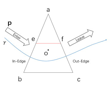
Figure 4: Moving across a triangle: the blue curve $\gamma$ notes the path of $p$ through $\Delta abc$; $p$ enters $\Delta abc$ through edge ab and leave it through edge ac.

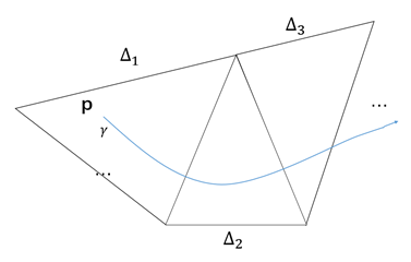
Figure 5: Moving through several triangles

3.3.4 Reward

The step reward for each agent is designed as the following:

$$r_{t}=r_{navigation}+r_{scenario}+r_{penalty}$$

Each agent gets a positive reward $r_{navigation}>0$ when it decides action $a_{0}$. The inspiration of setting so is to encourage the agent to get navigated as frequent as possible so that it can arrive at its target faster. The value of $\frac{{\pi}_{\theta}(a_{t}^{i}s_{t}^{i})}{{\pi}_{{\theta}_{old}}(a_{t}^{i}s_{t}^{i})}$ is set as,

$$r_{navigation}=\left\{\begin{aligned} &r_{0},&\ if\ decides\ a_{0}\\ &0,&else\end{aligned}\right.$$ (8)

The agent also gets a reward $r_{scenario}$ when interacting with the scenario. The idea is straightfoward: if the agent arrives at its target, it would get a positive reward; if it coolides, it would get a negative reward; otherwise, it would get nothing.

$$r_{scenario}=\left\{\begin{aligned} &r_{negative},&if\ collides\ with\ other\ objects\\ &r_{positive},&if\ arrives\ the\ target\\ &0,&else\end{aligned}\right.$$ (9)

Moreover, agent gets a time penalty $r_{penalty}<0$ at each time step. The maximal possible amount of time penalty that an agent can get in one single path shall be smaller than $T$. To ensure that the agent always gets a positive reward when it manages to arrive at its target, we assume that $r_{penalty}\cdot T\leq r_{positive}$.
In our experiments we set $r_{0}=0.00005,r_{negative}=-0.5,r_{positive}=1,r_{penalty}=-0.0001$.

3.3.5 Neural Network

Our approach is implemented with a parameter set $\theta\in R^{L}$ with scale $L$ for policy $\pi$. Here a linear neural network with $K$ full connection layers, each of $U=256$ units is employed. The input of this network is the observation gained by the sensors, and the output, the action of agent (Figure 6). The scale of parameter set $\theta$ is then $L=256*K$.

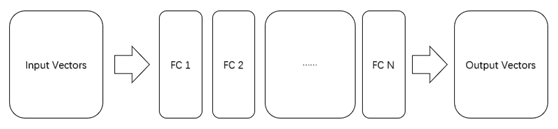
Figure 6: The neural network in our approach

3.3.6 Policy Gradient Method

In this work, we adopt a variation of the Policy Gradient Method [14].
Let $s_{t}\in\mathcal{S}$ be the state of the agent and $a_{t}\in\mathcal{A}$ the action taken by the agent at time step $t$. Let $V:\mathcal{s}\to\mathbb{R}$ be the value function of learning defined as

$$V(s)=\mathbb{E}[\sum_{t=0}^{\infty}\eta^{t}r_{t}|s_{0}=s]$$ (10)

where $\eta$ is the discount rate of learning.
The policy gradient method can be regarded as a stochastic gradient algorithm aiming at maximizing the following objective,

$$L(\theta)=\mathbb{E}\frac{{\pi}_{\theta}(a_{t}^{i}s_{t}^{i})}{{\pi}_{{\theta}_{old}}(a_{t}^{i}s_{t}^{i})}\hat{A}_{t}$$ (11)

where $\hat{A}_{t}$ is the advantage function [15] defined as the following:

$$\hat{A}_{t}=\delta_{t}+(\eta\lambda)\delta_{t+1}+...+(\eta\lambda)^{T-t+1}\delta_{T-1}$$ (12)

where $\delta_{t}=r_{t}+\eta V(s_{t+1})-V(s_{t})$. One can think of $\hat{A}_{t}$ as an analogy of the value function $V$ in classical reinforcement learning framework.
Then equation 11 leads to an estimator of policy gradient,

$$g(\theta)=\mathbb{E}\nabla_{\theta}\log\pi_{\theta}(a_{t}|s_{t})\hat{A}_{t}$$ (13)

where $\pi_{\theta}:\mathbb{S}\times\mathcal{A}\to\Delta(\mathcal{A})$ becomes a randomized policy that determines the distribution of $a_{t+1}$ according to $(s_{t},a_{t})$. In this work, the value function of policy $\pi$ is noted as $V(s;\pi_{\theta})$. The training process of each agent shares and updates the same parameter set $\theta$. $U$ is the batch size for data collecting. $\eta,\ \lambda,\ \epsilon$ are hyper-parameters of the algorithm. Their values will be introduced in section 4.

Algorithm 1 Proximal Policy Optimization (PPO, use clip surrogate objective)

1:for each episode with Max Training Step do

2:     for actor i= 1,2, …, N do

3:         Execute ${\pi}_{{\theta}_{old}}$ for U steps and gain $s_{t}^{i},\ a_{t}^{i},r_{t}^{i}$ respectively;

4:         Calculate advantage estimates $A_{1}^{i}…A_{t}^{i}$, according to formula:

$$A_{t}^{i}=\sum_{p=t}^{T-1}\{{(\eta\lambda)}^{p-t}[r_{p}^{i}+\eta V(s_{p+1}^{i};\pi_{\theta})-V(s_{p}^{i};\pi_{\theta})]\}$$

5:     end for

6:     Optimize $L(\theta)=min(u_{t}^{i}(\theta)A_{t}^{i},\ clip(u_{t}^{i}(\theta)A_{t}^{i},1-\epsilon,1+\epsilon)A_{t}^{i})\$using the Adam optimizer, where $u_{t}^{i}(\theta)=\frac{{\pi}_{\theta}(a_{t}^{i}s_{t}^{i})}{{\pi}_{{\theta}_{old}}(a_{t}^{i}s_{t}^{i})}$;

7:     ${\theta}_{old}\leftarrow\theta$ (All agents are updated in parallel)

8:end for

4 Simulation and Results

We begin this section by introducing the training scenario and hyper-parameters of our experiments. Then we turn to compare our methods quantitively with pure reinforcement learning methods [12], [13]. The section ends up with tests on some special scenarios.

4.1 Scenarios and Hyper-Parameters

Our algorithm is implemented in Tensorflow 1.4.0 (Python 3.5.2). The models of our scenarios and agents are built in Unity3D 2017.4.1f1. The policies are trained and simulated based on an i7-7500CPU and a NIVIDA GTX 950M GPU.
Our basic scenario is built in a square $\alpha$ of size 200 $\times$ 200 (Figure 7). Initially, $\alpha_{i},\beta_{i}$ are set randomly, and $v_{i}^{0}=(0,0)$, with $i=1,2,…,N$. We set $v_{0}=1,\ \omega_{0}=1,\ T=10000$ and $N=80$. Each agent will be reinitialized once it arrives its terminus point or its training exceeds the max training time step $T$. If a collision happens, the involved agents will also be immediately reinitialized. In the simulation, all the space, angle and velocity in the experiment adopt the basic units in Unity3D.

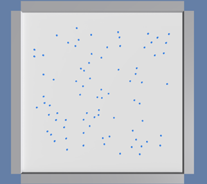
Figure 7: The Training Scenario

The hyper-parameters in table 1.

Hyper-Parameters	Value
$\eta$	0.99
$\lambda$	0.95
$\epsilon$	0.1
Hidden Units	256
Number of Full-Connection Layers	4 or 8
Max Training Step	5000000
Learning Rate	0.0003
Batch Size U	2048
Memory Size	2048

Table 3: The hyper-parameter list

The learning rate discounts as in 8.

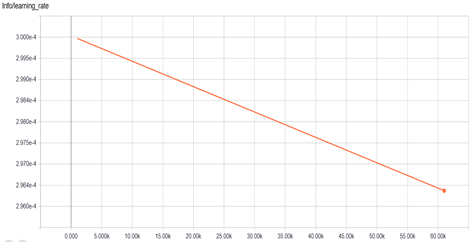
Figure 8: The Learning Rate Curve

4.2 Comparison: The Baseline Algorithm

To better demonstrate the performance of our method, we introduce a baseline algorithm [13],[14] and compare the simulation results between our method and this baseline algorithm.
The idea of its construction is straightfoward. One can regard this baseline algorithm as a "curtailed" version of our own algorithm in which the action $a_{0}$ is removed from the action set. In other words, this is an algorithm that involves nothing more than reinforcement learning. In the following content, we refer to it as "Pure Reinforcement Learning (RL) Method".

4.3 Results of Simulation

The result of training and test is shown as the following.

Several measurements are employed to quantitively measure the effectiveness of our approach in the training scenario and compare it with other methods in several scenarios. In our tests, a agent begins a trial once it is initialized or reinitialized. The trial ends if the agent arrives or collides with other objects. In the tests, we run the model in each scenario for 20000 trials and get the results.

1. Success Rate: In our experiment, a trial of a agent is said to be “success” once it arrives its terminus point without colliding others or exceeding max time step $T$. The success rate is defined as $\frac{Number\ of\ Sucess\ Trials}{Total\ Number\ of\ Trials}$.

2. Extra Distance Proportion (EDP): Since the starting points and terminus points are determined randomly, it is unreasonable to measure the circuitousness of the paths given by our method using average running distance or velocity of the agents. Hence, we adopt the Extra Distance Proportion (EDP). Given starting point $a$ and terminus point $b$ of a certain agent, suppose that $l$ is the shortest distance given by the pathfinding algorithm without considering avoiding its partner ($l$ could be precalculated before navigation, and in the training scenario we could obviously get $l=|a-b|$) and $d$ (obviously $d\geq l$) is the actual total distance the agent run in practice, the extra distance proportion $e(a,b)$ is defined as:

   $$e(a,b)=\frac{d-l}{l}$$

   We use $e$ to note the average EDP of all the agents during the test. We could easily see that the more circuitously the agent runs, the larger $e$ becomes. Note that EDP are only updated when one agent arrives its terminus point successfully.

3. Collision Rate: A trial ends and becomes an "accident" if the agent is involved in a collision. The collision Rate is defined as $\frac{Number\ of\ \ Accidents}{Total\ Number\ of\ Trials}$ during the test, reflecting the reliability of avoiding collision of the policy.

We train the agents with $N=80$, and test the policy when $N=40,80,120,160,200$ in the following scenarios. Our method (with 4 or 8 Full -Connection layers) are compared with the pure reinforcement learning approach in [12], [13]. In both cases, the models spend about 4 hours before converging to a stable policy. The 4-FC-layer policy converges after 22000 steps, while the 8-FC-layer case, 66000 steps. The pure RL policy spends 24 hours on training.
The learning process is also shown below. Figure 9 and Figure 10 are screen shots from Tensorboard. During the training, the Average Reward-Time ($r_{t}-t$) curve is adopted here to show the learning effectiveness of our algorithm.

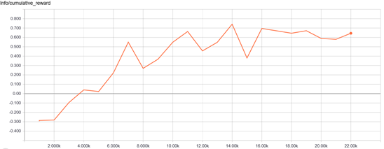
Figure 9: The Average Reward-Time Curve of our policy (4 FC layers)

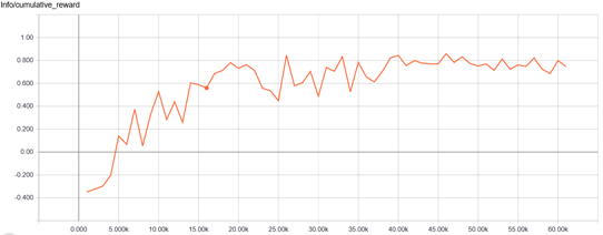
Figure 10: The Average Reward-Time Curve of our policy (4 FC layers)

1. Basic Scenario: This is our training scenario. During this test we also count the number of perceptible partners of each robot at each time step. We gain a sample of scale 100000 in the case $N=80,120,160,200$ and draw the histograms of them to show the crowdedness around individual agents. These statistics could partially reflect the variance of observation of agents while $N$ changes (Figure 11). Through these histograms we could see that what agents observe when $N=80$ largely differs from that when $N=160$ or $200$. This explains why the performance of our method decrease while $N$ increases, especially when $N$ exceeds 160;

2. Cross Road Scenario: This scenario is almost the same as the basic scenario. The only thing different is that each agent starts randomly from one of the four edges of $\alpha$ and is supposed to arrive a random point on the opposite edge. For instance, the agent may have starting point $a\in\left[x_{1},100\right]\subset S$and terminus point $b\in\left[x_{2},-100\right]\subset S$where $x_{1},\ x_{2}\in[-100,100]$. The results are shown in Table 2.

Our policy performances better than pure reinforcement learning methods in the tests. The agents can arrive at their terminus points with higher accuracy and lower cost. Meanwhile, our method learns much quicker compared to pure RL method and it does not require the agents to be retrained. It also shows better robustness in different cases, including different density of agents or different maps, especially when the scale of agents increases.
Next, we test the policy in different scenarios to show the adaptability for new scenarios of our approach. The results of these tests are shown in Table 3.

1. Four-Wall Scenario;

2. Random Obstacle Scenario;

3. Circle Transport scenario.

In those tests, the agents are capable of coping with unfamiliar scenarios without any further assistance. The value of EDP shows that our policy is able to optimize the paths of agents with lower computational cost, comparing to the pure RL method.

N	Method	Success Rate	EDP (mean/std)	Collision Rate
40	Pure RL Method Our Method (4 FC layers) Our Method (8 FC layers)	0.983 0.984 0.983	0.573/0.236 0.516/0.218 0.545/0.246	0.016 0.015 0.016
80	Pure RL Method Our Method (4 FC layers) Our Method (8 FC layers)	0.963 0.971 0.961	0.877/0.3252 0.652/0.281 0.701/0.2933	0.036 0.028 0.038
120	Pure RL Method Our Method (4 FC layers) Our Method (8 FC layers)	0.898 0951 0.921	0.987/0.477 0.854/0.403 0.866/0.425	0.093 0.047 0.077
160	Pure RL Method Our Method (4 FC layers) Our Method (8 FC layers)	0.732 0.862 0.860	1.132/0.532 1.054/0.456 0.991/0.481	0.138 0.136 0.137
200	Pure RL Method Our Method (4 FC layers) Our Method (8 FC layers)	0.532 0.831 0.783	1.232/0.738 1.126/0.653 1.103/0.689	0.249 0.167 0.211

Table 4: The results of tests in the basic scenario

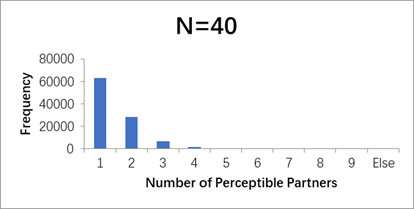
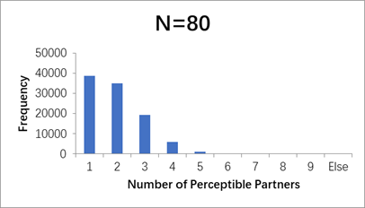
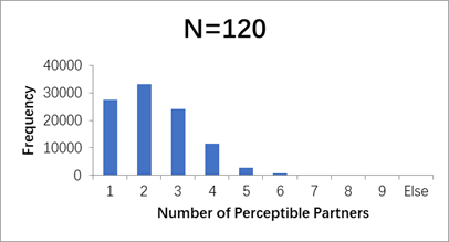
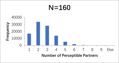
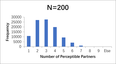
Figure 11: The crowdness when $N=40,80,120,160,200$

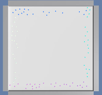
Figure 12: Cross Road Scenario

N	Method	Success Rate	EDP	Collision Rate
40	Pure RL Method Our Method (4 FC layers) Our Method (8 FC layers)	0.999 0.999 0.999	0.676/0.276 0.567/0.245 0.595/0.265	$<$0.001 $<$0.001 $<$0.001
80	Pure RL Method Our Method (4 FC layers) Our Method (8 FC layers)	0.921 0.999 0.999	1.021/0.323 0.759/0.293 0.756/0.301	0.053 $<$0.001 $<$0.001
120	Pure RL Method Our Method (4 FC layers) Our Method (8 FC layers)	0.865 0.992 0.973	1.352/0.501 0.861/0.412 0.959/0.454	0.082 0.007 0.025
160	Pure RL Method Our Method (4 FC layers) Our Method (8 FC layers)	0.742 0.945 0.923	1.932/0.572 1.030/0.478 1.054/0.492	0.142 0.054 0.071
200	Pure RL Method Our Method (4 FC layers) Our Method (8 FC layers)	0.632 0.914 0.889	2.214/0.784 1.171/0.677 1.170/0.709	0.232 0.085 0.109

Table 5: The results of tests in the cross-road scenario

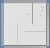
Figure 13: The Four-Wall(FW) Scenario: In this scenario, the blue agents start from $\{(x,y)|x\in 80,100,y\in[80,100]\}$ and are supposed to run to $\{(x,y)|x\in-80,-100,y\in[-80,-100]\}$; the pink agents do the opposite. Here we set $N=30$.

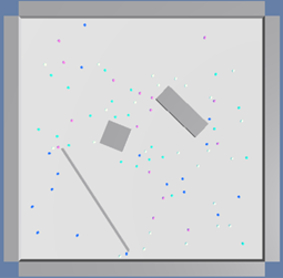
Figure 14: The Random Obstacle (RO) Scenario: This scenario contains several rectangle obstacles of random size. The starting and terminus points of agents are randomly set just like that in the cross road scenario. Here we set N=80, 120.

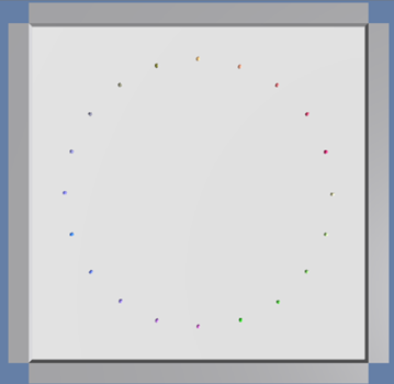
Figure 15: The Circle Transport (CT) Scenario: In this scenario, 20 agents are put uniformly on a circle of radius=80. Each of them are supposed to arrive its antipodal point. This is a difficult mission in multi-agent navigation, but the agents successfully finish the mission under the navigation.

Scenario	Method	Success Rate	EDP	Collision Rate
FW	Pure RL Method Our Method(4 FC layers)	0.329 0.969	2.313 1.177	0.360 0.030
RO N=80	Pure RL Method Our Method(4 FC layers)	0.623 0.999	1.951 0.833	0.268 $<$0.001
RO N=120	Pure RL Method Our Method(4 FC layers)	0.432 0.960	2.003 1.051	0.377 0.039
CT	Pure RL Method Our Method(4 FC layers)	0.999 0.999	1.310 0.893	$<$0.001 $<$0.001

Table 6: The performance of the policy that trained in our basic scenario in different scenarios

5 Conclusion

In this work, we develop a new framework for the multi-agent pathfinding and collision avoiding problem by combining a traditional pathfinding algorithm and a reinforcement learning method together. Both parts are essential–the reinforcement learning training determines the reliable behavior of the agents, while the pathfinding algorithm guarantees the arrival of them.
Numerical results demonstrate that our approach has a better accuracy and robustness compared to pure learning method. It is also adaptive for different scale of agents and scenarios without retraining.
Ongoing work will concentrate on enhancing the efficiency of our method by decreasing computational cost using tools in probability theory. Meanwhile, we are also interested in making use of the cooperation among agents to refine the framework of current algorithms.

References

- [1] W. Li, S. N. Chow, M. Egerstedt, J. Lu, and H. Zho, “Method of evolving junctions: A new approach to optimal path-planning in 2d environments with moving obstacles,” International Journal of Robotics Research, vol. 36, no. 4, p. 027836491770725, 2017.
- [2] P. E. Hart, N. J. Nilsson, and B. Raphael, “A formal basis for the heuristic determination of minimum cost paths,” IEEE Transactions on Systems Science and Cybernetics, vol. 4, no. 2, pp. 100–107, 2007.
- [3] R. B. Dial, “Algorithm 360: shortest-path forest with topological ordering [h],” Communications of the Acm, vol. 12, no. 11, pp. 632–633, 1969.
- [4] I. Debled-Rennesson, E. Domenjoud, B. Kerautret, and P. Even, Discrete Geometry for Computer Imagery. Springer, 2002.
- [5] D. Demyen and M. Buro, “Efficient triangulation-based pathfinding.” Aaai, vol. 1338, no. 9, pp. 161–163, 2007.
- [6] S. Bhattacharya, R. Ghrist, and V. Kumar, “Multi-robot coverage and exploration on riemannian manifolds with boundaries,” The International Journal of Robotics Research, vol. 33, no. 1, pp. 113–137, 2014.
- [7] W. Hönig, T. S. Kumar, L. Cohen, H. Ma, H. Xu, N. Ayanian, and S. Koenig, “Multi-agent path finding with kinematic constraints.” in ICAPS, vol. 16, 2016, pp. 477–485.
- [8] G. Sharon, R. Stern, A. Felner, and N. R. Sturtevant, “Conflict-based search for optimal multi-agent pathfinding,” Artificial Intelligence, vol. 219, pp. 40–66, 2015.
- [9] M. Sugiyama, H. Hachiya, and T. Morimura, Statistical Reinforcement Learning: Modern Machine Learning Approaches. Chapman & Hall/CRC, 2015.
- [10] T. Kohonen, “Self-organized formation of topologically correct feature maps,” Biological Cybernetics, vol. 43, no. 1, pp. 59–69, 1982.
- [11] Z. Liu, B. Chen, H. Zhou, G. Koushik, M. Hebert, and D. Zhao, “Mapper: Multi-agent path planning with evolutionary reinforcement learning in mixed dynamic environments,” arXiv preprint arXiv:2007.15724, 2020.
- [12] Y. F. Chen, M. Liu, M. Everett, and J. P. How, “Decentralized non-communicating multiagent collision avoidance with deep reinforcement learning,” pp. 285–292, 2016.
- [13] P. Long, T. Fan, X. Liao, W. Liu, H. Zhang, and J. Pan, “Towards optimally decentralized multi-robot collision avoidance via deep reinforcement learning,” 2017.
- [14] J. Schulman, F. Wolski, P. Dhariwal, A. Radford, and O. Klimov, “Proximal policy optimization algorithms,” 2017.
- [15] V. Mnih, A. P. Badia, M. Mirza, A. Graves, T. P. Lillicrap, T. Harley, D. Silver, and K. Kavukcuoglu, “Asynchronous methods for deep reinforcement learning,” 2016.
- [16] J. E. Godoy, I. Karamouzas, S. J. Guy, and M. Gini, “Adaptive learning for multi-agent navigation,” in Proceedings of the 2015 International Conference on Autonomous Agents and Multiagent Systems, 2015, pp. 1577–1585.
- [17] T. George Karimpanal and R. Bouffanais, “Self-organizing maps for storage and transfer of knowledge in reinforcement learning,” Adaptive Behavior, vol. 27, no. 2, p. 111C126, Dec 2018. [Online]. Available: http://dx.doi.org/10.1177/1059712318818568
- [18] J. Motes, R. Sandstrm, H. Lee, S. Thomas, and N. M. Amato, “Multi-robot task and motion planning with subtask dependencies,” IEEE Robotics and Automation Letters, vol. 5, no. 2, pp. 3338–3345, 2020.
- [19] F. Wang and E. Mckenzie, “A multi-agent based evolutionary artificial neural network for general navigation in unknown environments,” in Proceedings of the third annual conference on Autonomous Agents, 1999, pp. 154–159.
- [20] M. Hüttenrauch, A. Šošić, and G. Neumann, “Guided deep reinforcement learning for swarm systems,” 2017.
- [21] L. Tai, G. Paolo, and M. Liu, “Virtual-to-real deep reinforcement learning: Continuous control of mobile robots for mapless navigation,” in Ieee/rsj International Conference on Intelligent Robots and Systems, 2017.
- [22] G. Sartoretti, J. Kerr, Y. Shi, G. Wagner, T. S. Kumar, S. Koenig, and H. Choset, “Primal: Pathfinding via reinforcement and imitation multi-agent learning,” IEEE Robotics and Automation Letters, vol. 4, no. 3, pp. 2378–2385, 2019.
- [23] Y. Jiang, H. Yedidsion, S. Zhang, G. Sharon, and P. Stone, “Multi robot planning with conflicts and synergies,” Autonomous Robots, vol. 43, no. 8, pp. 2011–2032, 2019.
- [24] M. Gazzola, B. Hejazialhosseini, and P. Koumoutsakos, “Reinforcement learning and wavelet adapted vortex methods for simulations of self-propelled swimmers,” Siam Journal on Scientific Computing, vol. 36, no. 3, 2016.
- [25] C. E. Lemke and J. T. Howson, “Equilibrium points of bimatrix games,” Journal of the Society for Industrial & Applied Mathematics, vol. 12, no. 2, pp. 413–423, 1964.
- [26] Hu, Junling, Wellman, and P. Michael, “Nash q-learning for general-sum stochastic games,” Journal of Machine Learning Research, vol. 4, no. 4, pp. 1039–1069, 2003.