Equilibration of the Quark-Gluon Plasma at finite net-baryon density in QCD kinetic theory

Abstract

We explore the out-of-equilibrium dynamics of the Quark-Gluon Plasma at zero and finite net-baryon density based on an effective kinetic theory of Quantum Chromo Dynamics (QCD). By investigating the isotropization of the longitudinal pressure, we determine the relevant time and temperature scales for the onset of viscous hydrodynamics, and quantify the dependence on the chemical composition of the QGP. By extrapolating our results to realistic coupling strength, we discuss phenomenological consequences regarding the role of the pre-equilibrium phase at different collision energies.

Introduction —High-energy Heavy-Ion Collisions (HICs) at the Relativistic Heavy-Ion Collider (RHIC) and the Large Hadron Collider (LHC), provide a unique opportunity to explore the properties of strong interaction matter under extreme conditions. During the first ${\rm fm}/c$ of the space-time evolution of heavy-ion collisions, the non-equilibrium plasma of quarks and gluons created in the collision of heavy nuclei undergoes an out-of-equilibrium evolution Schlichting and Teaney (2019); Berges et al. (2020), before relativistic viscous hydrodynamics becomes applicable to describe the ensuing collective expansion of the near-equilibrium Quark-Gluon Plasma (QGP) Gale et al. (2013); Heinz and Snellings (2013). During the collective expansion, the hot and dense QGP is described in terms of macroscopic properties such as temperature $T$, chemical potentials $\mu$ and fluid velocity $u^{\mu}$ and cools down until on a time scale $\sim 10{\rm fm}/c$, the temperatures and densities approach the deconfinement transition of QCD, eventually leading to the production of the final state hadrons measured in the RHIC and LHC experiments.

Even though the early pre-equilibrium phase represents a rather short period of time during the complex space-time evolution of a heavy-ion collision, it is imperative to understand the pre-equilibrium evolution of the QGP in order to establish a complete theoretical description of the reaction dynamics. To this end, significant progress has been made in recent years towards understanding the equilibration and onset of hydrodynamic behavior in high temperature QCD plasmas, from holographic studies of supersymmetric theories Chesler and Yaffe (2009); Balasubramanian et al. (2011); Heller et al. (2012); Keegan et al. (2016) to weakly coupled Yang-Mills Kurkela and Lu (2014); Kurkela et al. (2019a); Heller et al. (2018); Almaalol et al. (2020) and QCD plasmas Kurkela and Mazeliauskas (2019) as well as in various models Blaizot and Yan (2020a, b, 2018); Kamata et al. (2020); Strickland (2018); Martinez et al. (2012); Kurkela et al. (2020); Behtash et al. (2020)

Despite clear differences at the microscopic level, a common finding of different theoretical approaches is that macroscopic properties of the system, such as the non-equilibrium evolution of the energy-momentum tensor $T^{\mu\nu}$, can be accurately described by relativistic viscous hydrodynamics on a time scale $\tau_{\rm hydro}$, long before the system approaches local thermal equilibrium on time scales $\tau_{\rm eq}\gg\tau_{\rm hydro}$. Strikingly, it has been also observed, that already at (very) early times $\tau\ll\tau_{\rm Hydro}$, the non-equilibrium evolution of macroscopic quantities may become insensitive to the details of the initial conditions, and can be effectively described in terms of non-equilibrium attractors Heller and Spalinski (2015); Romatschke (2018), which provides an accumulation point for the evolution of macroscopic quantities in out-of-equilibrium plasmas Behtash et al. (2019); Heller et al. (2020). While the existence of such attractors has been firmly established for different microscopic system undergoing a one-dimensional Bjorken expansion Heller and Spalinski (2015); Denicol and Noronha (2020); Romatschke (2018); Strickland et al. (2018); Strickland (2018); Giacalone et al. (2019); Almaalol et al. (2020); Heller et al. (2020), the study of non-equilibrium attractors remains an active research topic in theoretical physics and has lead to a number of interesting results Romatschke (2017); Behtash et al. (2020); Denicol and Noronha (2018, 2020) aiming to understand and extend the range of applicability of effective macroscopic descriptions, such as relativistic viscous hydrodynamics.

Beyond theoretical interest, the memory loss of macroscopic quantities also plays an important role in the phenomenological description of the pre-equilibrium stage of high-energy heavy-ion collisions , e.g. to quantify the (approximate) amount of entropy production during the early pre-equilibrium stage which is directly connected to experimental measurements of the charged particle multiplicity in the final state Giacalone et al. (2019), or to describe the space-time evolution of the pre-equilibrium plasma macroscopically in KoMPoST Kurkela et al. (2019a, b); Nunes da Silva et al. (2020); Gale et al. (2020).

So far investigations of the pre-equilibrium dynamics of the QGP have focused primarily on kinetic equilibration of pure glue QCD Kurkela and Lu (2014) with a recent extension to QCD Kurkela and Mazeliauskas (2019) for charge neutral plasmas. By performing numerical simulations of the leading order effective kinetic theory of QCD Arnold et al. (2003) for gluons and light flavor $(u,d,s)$ quarks, we extend the theoretical treatment of the pre-equilibrium description QGP for the first time to finite net charge/net baryon density. We investigate the existence of non-equilibrium attractors and describe their phenomenological consequences in the theoretical description of the pre-equilibrium stage. Within this letter, we focus on the aspects most relevant to heavy-ion phenomenology, and refer to our companion paper Du and Schlichting (2020) for a detailed exposition of the theoretical framework and additional discussions.

Effective kinetic description of pre-equilibrium dynamics — During the collision of heavy nuclei a fraction of the energy and valence charge is deposited in a primordial plasma, providing the initial conditions for the subsequent pre-equilibrium evolution of the QGP. In high-energy collisions the Color Glass Condensate (CGC) effective field theory of high-energy QCD Gelis et al. (2010); Iancu and Venugopalan (2003), provides a theoretical description of the gluon dominated initial state created at very early times Kovner et al. (1995); Krasnitz and Venugopalan (1999); Krasnitz et al. (2003); Blaizot et al. (2010); Schenke et al. (2012). Despite recent efforts to generalize this framework to include quark production Gelis and Tanji (2016); Fujii et al. (2006); Gelis et al. (2006), baryon stopping McLerran et al. (2019) and other corrections to the high-energy limit Lushozi et al. (2020); Kajantie et al. (2020); Agostini et al. (2019), so far the chemical composition of the non-equilibrium plasma, as well as the structure of non-equilibrium initial state in heavy-ion collisions at lower beam energies or the forward rapidity regions of high energy collisions is currently not well understood. We will therefore consider a rather generic parametrization of the initial phase-space distributions of gluons, quarks and anti-quarks

$$f_{g}(\tau_{0},p_{T},p_{\|}) =f^{0}_{g}\frac{Q_{0}}{\sqrt{p_{T}^{2}+\xi_{0}^{2}p_{\|}^{2}}}e^{-\frac{2(p_{T}^{2}+\xi_{0}^{2}p_{\|}^{2})}{3Q_{0}^{2}}}\;,$$ (1)

$$f_{q_{f}/\bar{q}_{f}}(\tau_{0},p_{T},p_{\|}) =f^{0}_{q_{f}/\bar{q}_{f}}\frac{\sqrt{p_{T}^{2}+p_{\|}^{2}}}{\sqrt{p_{T}^{2}+\xi_{0}^{2}p_{\|}^{2}}}e^{-\frac{2(p_{T}^{2}+\xi_{0}^{2}p_{\|}^{2})}{3Q_{0}^{2}}}\;.$$

where the initial abundance of the $N_{f}=3$ light flavor quarks and anti-quarks is determined by the sum of the contributions from valence quark stopping ($f_{v}^{0}$) and quark/anti-quark pair production ($f_{0}^{s}$) as

$$f^{0}_{u} =\frac{2n_{p}+n_{n}}{3(n_{p}+n_{n})}f_{v}^{0}+\frac{1}{2N_{f}}f_{s}^{0}\;,\qquad f^{0}_{\bar{u}}=\frac{1}{2N_{f}}f_{s}^{0}\;,$$

$$f^{0}_{d} =\frac{n_{p}+2n_{n}}{3(n_{p}+n_{n})}f_{v}^{0}+\frac{1}{2N_{f}}f_{s}^{0}\;,\qquad f^{0}_{\bar{d}}=\frac{1}{2N_{f}}f_{s}^{0}\;,$$

$$f^{0}_{s} =\frac{1}{2N_{f}}f_{s}^{0}\;,\qquad\qquad\qquad f^{0}_{\bar{s}}=\frac{1}{2N_{f}}f_{s}^{0}\;,$$ (2)

with $n_{p}/n_{n}=2/3$ denoting the proton/neutron fraction of the colliding nuclei. We will vary the parameters $\xi_{0}$ representing the initial momentum anisotropy, as well as $f^{0}_{g}$,$f^{0}_{s}$ and $f^{0}_{v}$ to investigate the sensitivity of our results to the initial conditions.

Starting from the above initial conditions, we solve the QCD Boltzmann equation Mueller (2000)

$$\left[\frac{\partial}{\partial\tau}-\frac{p_{\|}}{\tau}\frac{\partial}{\partial p_{\|}}\right]f_{a}(\tau,p_{T},p_{\|})=$$ (3)

$$\qquad-C^{{2\leftrightarrow 2}}_{a}[f](\tau,p_{T},p_{\|})-C^{{1\leftrightarrow 2}}_{a}[f](\tau,p_{T},p_{\|})\;,$$

for a (longitudinally) boost invariant (transversely) homogeneous system undergoing a one dimensional Bjorken expansion. We include all leading order elastic $(C^{{2\leftrightarrow 2}})$ and inelastic $(C^{{1\leftrightarrow 2}})$ interactions, and following previous works Kurkela et al. (2019b); Kurkela and Mazeliauskas (2019) account for in-medium screening of elastic interactions Arnold et al. (2003) and the Landau-Pomeranchuk-Migdal Landau and Pomeranchuk (1953a, b); Migdal (1955) suppression of inelastic rates, as described in detail in our companion paper Du and Schlichting (2020).

Non-equilibrium evolution of macroscopic properties — In order to connect the non-equilibrium initial state, with the subsequent hydrodynamic evolution we will focus on the pre-equilibrium evolution of the macroscopic properties of the QGP. Specifically, we will investigate the evolution of the energy momentum tensor $T^{\mu\nu}$ and conserved currents $J^{\mu}_{f}$, determined as

$$T^{\mu\nu} = \int\frac{d^{3}p}{(2\pi)^{3}}\frac{p^{\mu}p^{\nu}}{p}\left[\nu_{g}f_{g}(\vec{p})+\nu_{q}\sum_{f}\left(f_{q_{f}}(\vec{p})+f_{\bar{q}_{f}}(\vec{p})\right)\right]\;,$$

$$\Delta J^{\mu}_{f} = \int\frac{d^{3}p}{(2\pi)^{3}}\frac{p^{\mu}}{p}\left[\nu_{q}\left(f_{q_{f}}(\vec{p})-f_{\bar{q}_{f}}(\vec{p})\right)\right]\;.$$ (4)

Based on the symmetries of the one-dimensional Bjorken expansion, one finds that in Milne $(\tau,x,y,\eta)$ coordinates $T^{\mu\nu}=\text{diag}(e,p_{T},p_{T},\frac{p_{L}}{\tau^{2}})$, $\Delta J^{\nu}_{f}=(\Delta n_{f},0,0,0)$ in the local rest-frame $u^{\mu}=(1,0,0,0)$, and the conservation laws take the form

$$\partial_{\tau}e+\frac{e+p_{L}}{\tau}=0\;,\qquad\partial_{\tau}\Delta n_{f}+\frac{\Delta n_{f}}{\tau}=0,$$ (5)

such that irrespective of the underlying microscopic dynamics, the charge density per unit rapidity $\tau\Delta n_{f}=(\tau\Delta n_{f})_{0}=(\tau\Delta n_{f})_{\rm eq}$ remains constant throughout the evolution. Conversely, the evolution of the energy density $e$ is affected by the longitudinal pressure $p_{L}$. Due to the rapid longitudinal expansion, the longitudinal pressure $p_{L}\ll e$ is initially much smaller than the transverse pressure $p_{T}\simeq e/2$, resulting in a constant ratio of energy per baryon $e/\Delta n_{B}$ and a constant energy density per unit rapidity $(e\tau)_{0}$ at early times.

Over the course of the non-equilibrium evolution, the longitudinal expansion slows down, while kinetic interactions lead to a continuous increase of the longitudinal pressure $p_{L}$ (c.f. Fig. 1). Eventually, the residual deviations from equilibrium can be captured by hydrodynamic constitutive relations, where to first order in the gradient expansion the longitudinal pressure is determined by

$$\frac{p_{L}}{e}=\frac{1}{3}-\frac{16}{9}\frac{\eta}{(e+p)\tau}$$ (6)

with shear-viscosity $\eta$ and thermodynamic pressure $p=e/3$ for a conformal plasma. Ultimately, the QGP approaches an isotropic equilibrium state ($p_{L}=p_{T}=e/3$) where energy and charge densities are described by temperature $T$ and chemical potentials $\mu_{f}$ as

$$e_{\rm eq} = \left[\nu_{g}\frac{\pi^{2}}{30}+\nu_{q}\frac{\pi^{2}}{120}\sum_{f}\left(7+\frac{30}{\pi^{2}}\frac{\mu_{f}^{2}}{T^{2}}+\frac{15}{\pi^{4}}\frac{\mu_{f}^{4}}{T^{4}}\right)\right]T^{4}\;,$$

$$\Delta n_{f,eq} = \frac{\nu_{q}}{6}\left[\frac{\mu_{f}}{T}+\frac{1}{\pi^{2}}\frac{\mu_{f}^{3}}{T^{3}}\right]T^{3}$$ (7)

for an ultra-relativistic plasma of quarks and gluons, such that $\tau^{4/3}e$ and $\mu_{f}/T$ approach constant values $(\tau^{4/3}e)_{\rm eq}$, $(\mu_{f}/T)_{\rm eq}$ at late times $\tau\gg\eta/(e+p)$ when the QGP approaches local thermal equilibrium.

$Q_{0}\tau_{0}$	$f_{g}^{0}$	$f_{val}^{0}$	$f_{split}^{0}$	$\xi_{0}$	$(\frac{\mu_{B}}{T})_{\rm eq}$	$\left(\frac{\eta T_{\rm eff}}{e+p}\right)$	$C_{\infty}$
9.9	1.068	0	0	10	0	1.00	0.91
9.9	1.068	0	0	5	0	1.00	0.93
9.9	1.068	0	0	20	0	1.00	0.91
9.9	0.950	0	0.269	10	0	1.00	0.92
9.9	0.833	0	0.534	10	0	1.00	0.94
9.9	0.598	0	1.068	10	0	1.00	0.96
9.9	0.363	0	1.602	10	0	1.00	0.98
9.9	0	0	2.427	10	0	1.00	1.01
9.9	0.950	0.269	0	10	0.34	1.01	0.93
9.9	0.833	0.534	0	10	0.67	1.01	0.94
9.9	0.598	1.068	0	10	1.31	1.03	0.96
9.9	0.598	1.068	0	5	1.31	1.03	0.98
9.9	0.598	1.068	0	20	1.31	1.03	0.96
9.9	0.363	1.602	0	10	1.93	1.06	0.98
22.5	0.363	1.602	0	10	2.38	1.08	1.08
22.5	0.363	1.602	0	5	2.38	1.08	1.11
22.5	0.363	1.602	0	20	2.38	1.08	1.08

Table 1: Summary of initial conditions for QCD kinetic theory simulations for coupling strength $\lambda=g^{2}N_{c}=10$ along with the values of $(\mu_{B}/T)_{\rm eq}$, $(\eta T_{\rm eff})/(e+p)$ and $C_{\infty}$ extracted from fits to the asymptotic behavior of $\Delta n_{f}/e^{3/4}$ in Eq. (Equilibration of the Quark-Gluon Plasma at finite net-baryon density in QCD kinetic theory), $p_{L}/e$ in Eq. (6) and $(\tau^{4/3}e)/(\tau^{4/3}e)_{\rm eq}$ in Eq. (Equilibration of the Quark-Gluon Plasma at finite net-baryon density in QCD kinetic theory).

We present our results for the non-equilibrium evolution of the long. pressure to energy density ratio in Fig. 1, where we show the time evolution of $p_{L}/e$ for different initial conditions at zero and non-zero net-baryon density summarized in Tab. 1. Starting from a highly anisotropic initial state at early times, the longitudinal pressure soon exhibits a rapid rise, followed by a slow approach towards isotropy $(p_{L}/e=1/3)$ at late times.

Strikingly, previous studies of the pressure isotropization in pure glue QCD Kurkela and Lu (2014); Kurkela et al. (2019b, a) and QCD at zero density Kurkela and Mazeliauskas (2019) have shown, that the non-equilibrium evolution of the energy momentum tensor at different coupling strength is governed by a universal scaling variable $\tilde{w}=\frac{\tau T}{4\pi\eta/s}$ Heller et al. (2018); Giacalone et al. (2019), representing the ratio of the evolution time $\tau$, to the the equilibrium relaxation time $\tau_{R}=\frac{4\pi\eta/s}{T}$. By introducing an effective temperature $T_{\rm eff}=\left(\frac{30e(\tau)}{\pi^{2}\nu_{\rm eff}}\right)^{\frac{1}{4}}$ with $\nu_{\rm eff}=\nu_{g}+\frac{7}{4}\nu_{q}N_{f}$ characterizing the energy density of the non-equilibrium QGP, the definition of the scaling variable can be generalized to finite density systems as

$$\tilde{\omega}=\frac{(e+p)\tau}{4\pi\eta}=\left(\frac{e+p}{\eta T_{\rm eff}}\right)\frac{\tau T_{\rm eff}}{4\pi}$$ (8)

such that the hydrodynamic evolution of the pressure in Eq. (6) remains a universal function of the scaling variable $\frac{p_{L}}{e}=\frac{1}{3}-\frac{4}{9\pi\tilde{\omega}}$, irrespective of the net-baryon density. Indeed one observes from Fig. 1 that eventually all curves converge towards the same viscous hydrodynamic behavior, which provides an accurate description of the pressure anisotropy for $\tilde{w}\gtrsim 1$. We note that albeit, the dimensionless transport coefficient $\left(\frac{\eta T_{\rm eff}}{e+p}\right)$, which at zero density reduces to $\eta/s$, exhibits a chemical potential dependence, we find that the variations of $\left(\frac{\eta T_{\rm eff}}{e+p}\right)$ are only at the $10\%$ level for the considered range of chemical potentials $(\mu_{B}/T)_{\rm eq}\lesssim 2.5$, as can be seen from Tab. 1, where we provide the results for $\left(\frac{\eta T_{\rm eff}}{e+p}\right)$ extracted from fits to the late time asymptotics of $p_{L}/e$ in Eq. (6).

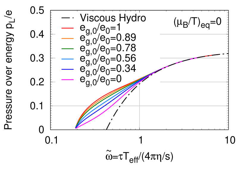
Figure 1: Non-equilibrium evolution of the longitudinal pressure over energy ratio $\frac{p_{L}}{e}$ for different net-baryon density (top) and different initial quark to gluon ratios at zero density (bottom). Dotted and dashed curves in the top panel show results for different initial anisotropies $\xi_{0}$.

Despite their common late time behavior, some important differences emerge in the evolution of the pressure anisotropy at intermediate times ($\tilde{w}\lesssim 1$). By comparing the solid and dashed curves in the top panel of Fig. 1, we find that variations of the initial momentum anisotropy $\xi_{0}$ do not significantly affect the evolution of the pressure beyond very early times, which is in line with detailed earlier investigation in pure glue QCD Almaalol et al. (2020). Conversely, changes in the chemical composition of the primordial plasma do have a noticeable effect on the isotropization of the pressure at intermediate times, resulting in a moderate dependence on the net-baryon density $\mu_{B}/T$ shown in the top panel of Fig. 1. Generally, the isotropization of the pressure proceeds more and more slowly the larger the quark fraction, which is in line with early theoretical expectations Biro and Zimanyi (1982), attributing the slower equilibration of the quark sector to the differences in color factors in elastic and inelastic scattering processes. Even in zero density systems, shown in the bottom panel of Fig. 1, the initial quark/gluon fraction affects the evolution of the pressure at intermediate times $\tilde{w}\lesssim 1$, challenging the existence of a universal non-equilibrium attractor, where the evolution of the pressure anisotropy becomes insensitive to the details of the initial conditions before the onset of hydrodynamic behavior Romatschke (2018); Strickland (2018); Kurkela et al. (2019b); Kurkela et al. (2020); Almaalol et al. (2020). Nevertheless, the variations of $p_{L}/e$ are still rather moderate, and it is equally important to point out that by the time $\tilde{w}\sim 1$ where hydrodynamics becomes applicable, differences in the initial chemical composition no longer effect the pressure evolution.

Connecting the initial state to hydrodynamics — Now that we have established the evolution of the pressure anisotropy during the early pre-equilibrium phase, we can determine how the initial energy density $(e\tau)_{0}$ and net-charge density $(\Delta n_{f}\tau)_{0}$ affect the initial conditions for the subsequent hydrodynamic evolution. By following the arguments of Giacalone et al. (2019), the evolution of the conserved quantities $e$ and $\Delta n_{f}$ during the pre-equilibrium phase can be compactly expressed as

$$\left(\tau^{\frac{4}{3}}e\right)(\tilde{\omega}) = \left(4\pi\frac{\eta T_{\rm eff}}{e+p}\right)^{\frac{4}{9}}\left(\frac{\pi^{2}\nu_{\rm eff}}{30}\right)^{\frac{1}{9}}(e\tau)_{0}^{\frac{8}{9}}C_{\infty}\mathcal{E}(\tilde{\omega})\;,$$

$$\left(\tau\Delta n_{f}\right)(\tilde{\omega}) = \left(\tau\Delta n_{f}\right)_{0}\;,$$ (9)

where as explained in the supplemental material, the function $\mathcal{E}(\tilde{\omega})=\frac{\tau^{4/3}e(\tau)}{(\tau^{4/3}e)_{\rm eq}}$ describes the non-trivial evolution of the energy density due to work performed against the longitudinal expansion Bjorken (1983); Gyulassy and Matsui (1984); Giacalone et al. (2019). Specifically, at early and late times $\mathcal{E}(\tilde{\omega})$ has the asymptotic behavior

$$\mathcal{E}(\tilde{\omega}\gg 1)\simeq 1-\frac{2}{3\pi\tilde{\omega}}\qquad(\text{visc. hydro})$$

$$\mathcal{E}(\tilde{\omega}\ll 1)\simeq C_{\infty}^{-1}{\tilde{\omega}}^{\frac{4}{9}}\qquad(\text{free-streaming})$$ (10)

such that the constant $C_{\infty}$ in Eqns. (Equilibration of the Quark-Gluon Plasma at finite net-baryon density in QCD kinetic theory) and (Equilibration of the Quark-Gluon Plasma at finite net-baryon density in QCD kinetic theory) describes the efficiency with which the initial energy density per unit-rapidity $(e\tau)_{0}$ is converted into the thermal energy density at the onset of hydrodynamics.

Due to the different evolution of the pressure anisotropy, this conversion is different between zero and finite density systems, as can be seen in Fig. 2, where we present our results for the non-equilibrium evolution of the energy density of the QGP at different values of the baryon chemical potential $(\mu_{B}/T)_{\rm eq}$ at late times. Evidently the more baryon rich systems experience a smaller longitudinal pressure during the pre-equilibrium phase and therefore converts the initial energy density more efficiently into thermal energy. By matching the results from our QCD kinetic theory simulations to the asymptotic behavior in Eq. (Equilibration of the Quark-Gluon Plasma at finite net-baryon density in QCD kinetic theory), we have extracted the values of $C_{\infty}$ to quantify this effect and provide the respective values for all simulations in Tab. 1. We find that for the considered range of parameters, the dependence on the chemical composition of the primordial plasma is typically on the $10-15\%$ level, indicating that despite the differences in the pressure evolution, the energy density at the beginning of the hydrodynamics phase can still be estimated to a rather good accuracy.

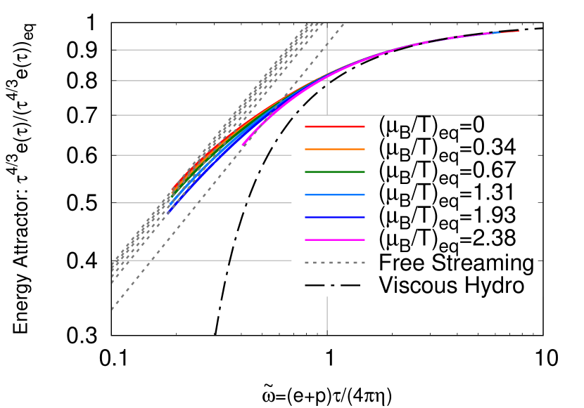
Figure 2: Non-equilibrium evolution of the energy density for different net-baryon densities, characterized by the ratio of the chemical potentials to temperature $(\mu_{B}/T)_{\rm eq}$ at late times. Dashed and solid curves show a comparison to early and late time asymptotics in Eq. (Equilibration of the Quark-Gluon Plasma at finite net-baryon density in QCD kinetic theory).

Phenomenological consequences — We conclude our analysis by studying the phenomenological consequences of our results, for the dynamical description of heavy-ion collision experiments at RHIC and LHC energies. Neglecting the entropy production during the late stage hydrodynamic expansion, we follow previous works Giacalone et al. (2019); Jankowski et al. (2020) matching the asymptotic entropy density

$$(\tau s)_{\rm eq}=\frac{4}{3}\frac{(e\tau^{4/3})_{\rm eq}}{(\tau^{1/3}T)_{\rm eq}}-\left(\frac{\mu_{B}}{T}\right)_{\rm eq}\Delta n_{B}-\left(\frac{\mu_{Q}}{T}\right)_{\rm eq}\Delta n_{Q}\;,$$ (11)

to the experimentally measured charged particle multiplicities, according to $dN_{\rm ch}/d\eta=\frac{N_{\rm ch}}{S}(\tau s)_{\rm eq}S_{\bot}$, and fix the final entropy to baryon number ratio $(\tau s)_{\rm eq}/(\tau\Delta n_{B})_{\rm eq}$, according to $\Delta n_{B}/s$=144, 285, 420 for 62.4 GeV, 130 GeV, 200 GeV Au+Au collisions. We employ $S/N_{\rm ch}=8.36$  Giacalone et al. (2019); Hanus et al. (2019) and estimate the transverse area $S_{\bot}=\pi R_{A}^{2}$=128 fm², 138 fm², 95 fm² for central Au+Au, Pb+Pb, Xe+Xe collisions with $dN_{\rm ch}/d\eta$=470, 590, 665 for 62.4 GeV, 130 GeV, 200 GeV Au+Au collisions; $dN_{\rm ch}/d\eta$=1600, 1942 for 2.76 TeV, 5.02 TeV Pb+Pb collisions, $dN_{\rm ch}/d\eta$=1166 for 5.44 TeV Xe+Xe collision Arsene et al. (2005); Back et al. (2006); Aamodt et al. (2011). Since the overall normalization is fixed by this procedure, Eq. (Equilibration of the Quark-Gluon Plasma at finite net-baryon density in QCD kinetic theory) then provides the evolution of the energy $e$ and charge densities $\Delta n_{f}$, from which we infer temperatures $T$ and baryon chemical potential $\mu_{B}$ based on the usual Landau matching procedure associating the conserved charges with their equilibrium values $e=e_{\rm eq}(T,\mu_{f})$ and $\Delta n_{f}=n_{\rm eq}(T,\mu_{f})$.

We illustrate the resulting non-equilibrium trajectories of the QGP in the QCD phase-diagram in Fig. 3, where dashed (dotted) lines represent the pre-hydrodynamic evolution of $(T,\mu_{B})$ for $0.2<\tilde{\omega}<1$, whereas solid lines show the hydrodynamic trajectories for $\tilde{\omega}>1$ for two different values of the transport coefficient $\eta T_{\rm eff}/(e+p)$=0.08 (0.16). Strikingly, one observes at first sight, that the pre-equilibrium plasma can exhibit much higher temperatures and chemical potentials as can be achieved during the subsequent hydrodynamic evolution. While in high-energy collisions of heavy nuclei, the trajectories run straight down along the vertical axis $(\mu_{B}/T\approx 0)$, the non-equilibrium trajectories at lower energies bend towards larger values of $\mu_{B}/T$ and deviate significantly from the (perturbative) isentropes indicated by gray dotted lines.

Concerning the applicability of hydrodynamics, one finds that e.g. in high-energy Pb+Pb collisions, the hydrodynamic description becomes applicable on time scales

$$\tau \simeq 1.3~{}{\rm fm}/c\left(\frac{4\pi\eta/s}{2}\right)^{\frac{3}{2}}\left(\frac{dN_{ch}/d\eta}{1942}\right)^{-\frac{1}{2}}\left(\frac{S_{\bot}}{138{\rm fm}^{2}}\right)^{\frac{1}{2}}$$

and temperatures

$$T \simeq 300{\rm MeV}\left(\frac{4\pi\eta/s}{2}\right)^{-\frac{1}{2}}\left(\frac{dN_{ch}/d\eta}{1942}\right)^{\frac{1}{2}}\left(\frac{S_{\bot}}{138{\rm fm}^{2}}\right)^{-\frac{1}{2}}$$ (12)

well above the QCD cross-over temperature $T_{c}\simeq$156 MeV Bazavov et al. (2019), indicated by a black line in Fig. 3. However, at lower energies the non-equilibrium trajectories extend almost all the way to the QCD phase boundary, indicating that the QGP created in low energy collisions may be significantly out of equilibrium for a substantial part of its lifetime. Even though the use of a perturbative description and the modeling of the space-time dynamics in terms of a one dimensional Bjorken expansion become increasingly questionable at lower energies, we still believe that Fig. 3 points to one of several important challenges in describing the space-time evolution of heavy-ion collisions at low energies Romatschke (2010); Gale et al. (2013); Yan (2018); Shen and Yan (2020); Dore et al. (2020).

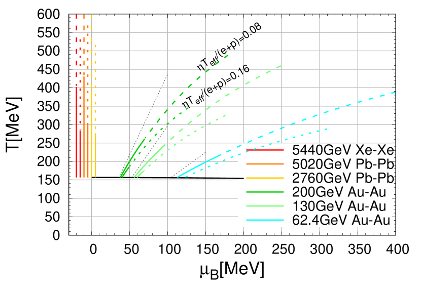
Figure 3: Non-equilibrium trajectories of temperature $T$ and baryon chemical potential $\mu_{B}$ in the QCD phase-diagram for $0-5\%$ most central heavy-ion collisions. Dashed/dotted lines show the pre-equilibrium evolution $0.2<\tilde{w}<1$ for $\eta T_{\rm eff}/(e+p)$=0.08, 0.16, while solid lines correspond to the hydrodynamic evolution for $\tilde{w}>1$ which approaches the (perturbative) isentropes indicated by gray dashed lines. Black solid line indicates the QCD cross over temperature $T_{c}$=156.5 MeV Bazavov et al. (2019).

Conclusions & Outlook — We investigated the early time pre-equilibrium dynamics of the QGP at zero and finite densities of the conserved baryon and electric charge based on an effective kinetic description of high-energy QCD. We find that for a plasma undergoing a one dimensional Bjorken expansion, the non-equilibrium evolution of the energy momentum tensor can be well described by viscous hydrodynamics for time $\tau\gtrsim\frac{4\pi\eta}{e+p}$, which is in accordance with earlier findings at zero density Kurkela and Mazeliauskas (2019). However, the chemical composition of the QGP can have a significant impact on the evolution of the pressure at early times $\tau\lesssim\frac{4\pi\eta}{e+p}$, which is in sharp contrast to the results obtained for single component plasmas Heller et al. (2012); Keegan et al. (2016); Kurkela and Lu (2014); Heller and Spalinski (2015); Kurkela et al. (2019a); Heller et al. (2018); Almaalol et al. (2020); Berges et al. (2014a, b); Kamata et al. (2020); Strickland (2018); Denicol and Noronha (2020); Romatschke (2018); Strickland et al. (2018); Heller et al. (2020), where macroscopic properties such as $p_{L}/e$ exhibits a rapid memory loss at early times, resulting in a universal approach towards viscous hydrodynamics. Even though, the ensuing differences in the pressure only affect the late time evolution of the QGP at the $10-15\%$ level, it is clear that further progress in the theoretical understanding hinges to a considerable extent on an improved determination of the chemical composition of the primordial plasma, created immediately after the collision of heavy nuclei.

We further discussed how the results presented in this letter can be used to connect the properties of the non-equilibrium initial state to the initial conditions for the subsequent hydrodynamic evolution. By extending previous works Giacalone et al. (2019) to include the effects of finite net-baryon and electric charge density, our calculations thus provide a first important step towards including the evolution of all QCD conserved charges into dynamical descriptions of the pre-equilibrium stage of heavy-ion collisions Kurkela et al. (2019a, b); Martinez et al. (2019). Beyond such applications to bulk phenomenology, our QCD kinetic theory studies also provide the basis for future investigations of heavy flavor dynamics or the emission of electromagnetic probes, which could provide sensitive probes of the early time non-equilibrium dynamics Churchill et al. (2020); Kasmaei and Strickland (2019, 2020).

Acknowledgement — We thank Giuliano Giacalone and Aleksas Mazeliauskas for many insightful discussions and valuable contributions to the supplemental material. We further thank Aleksi Kurkela, Jean-Francois Paquet, Ismail Soudi and Derek Teaney for insightful discussions and collaboration on related projects. This work is supported by the Deutsche Forschungsgemeinschaft (DFG, German Research Foundation) – project number 315477589 – TRR 211. The authors also acknowledge computing time provided by the Paderborn Center for Parallel Computing (PC2) and the National Energy Research Scientific Computing Center, a DOE Office of Science User Facility supported by the Office of Science of the U.S. Department of Energy under Contract No. DE-AC02-05CH11231.

Supplemental material

Below we provide a brief re-derivation of Eq. (Equilibration of the Quark-Gluon Plasma at finite net-baryon density in QCD kinetic theory) which, as originally derived in Ref. Giacalone et al. (2019), relates the initial energy density to the initial conditions for the subsequent hydrodynamic evolution. Denoting $p_{L}/e=f(\tilde{\omega})$ in the following with $\tilde{\omega}=\frac{T_{\rm eff}(\tau)\tau}{4\pi\eta/s}$ as in Eq. (8), the energy conservation equation can be re-cast into the form

$$\tau\partial_{\tau}e=-e(1+f(\tilde{\omega}))\;,$$ (13)

Based on the knowledge of $p_{L}/e$, one can then directly integrate out the conservation equation. By changing variables from $\tau$ to $\tilde{\omega}$ according to

$$\tau\partial_{\tau}=a(\tilde{\omega})\tilde{\omega}\partial_{\tilde{\omega}}\;,\qquad a(\tilde{\omega})=\frac{3}{4}-\frac{1}{4}f(\tilde{\omega})$$ (14)

one obtains

$$e(\tilde{\omega}_{\tau})=e(\tilde{\omega}_{0})\exp\left(-\int_{\tilde{\omega}_{0}}^{\tilde{\omega}_{\tau}}\frac{d\tilde{\omega}}{\tilde{\omega}}\frac{1+f(\tilde{\omega})}{a(\tilde{\omega})}\right).$$ (15)

Now in order to turn this into a more practical formula, it is useful to factor our the asymptotic behavior at early and late times, where obviously

$$e(\tilde{\omega}\gg 1)\propto\tilde{\omega}^{-2}$$ (16)

$$e(\tilde{\omega}\ll 1)\propto\tilde{\omega}^{-\frac{4}{3}}$$ (17)

By considering the ratio $\frac{\tilde{\omega}_{\tau}^{2}e(\tilde{\omega}_{\tau})}{\tilde{\omega}_{0}^{\frac{4}{3}}e(\tilde{\omega}_{0})}$, and making use of the relation between the energy density and the effective temperature $e(\tilde{\omega})=\frac{\pi^{2}}{30}\nu_{\rm eff}T_{\rm eff}^{4}(\tilde{\omega})$ to re-express additional powers of temperature in terms of additional powers of energy, one arrives at

$$\tau^{\frac{4}{3}}e(\tau) = \left(4\pi\frac{\eta T_{\rm eff}}{e+p}\right)^{\frac{4}{9}}\left(\frac{\pi^{2}}{30}\nu_{\rm eff}\right)^{\frac{1}{9}}\left(e\tau\right)_{0}^{\frac{8}{9}}$$

$$\times\left[\frac{\tilde{\omega}_{\tau}^{2}}{\tilde{\omega}_{0}^{\frac{4}{3}}}\exp\left(-\int_{\tilde{\omega}_{0}}^{\tilde{\omega}_{\tau}}\frac{d\tilde{\omega}}{\tilde{\omega}}\frac{1+f(\tilde{\omega})}{a(\tilde{\omega})}\right)\right]^{\frac{2}{3}}$$

where the expression in the square bracket is constructed in such a way that the limits $\tilde{\omega}_{\tau}\to\infty$ and $\tilde{\omega}_{0}\to 0$ are finite, yielding

$$C_{\infty}=\lim_{\tilde{\omega}_{\tau}\to\infty,\tilde{\omega}_{0}\to 0}\left[\frac{\tilde{\omega}_{\tau}^{2}}{\tilde{\omega}_{0}^{\frac{4}{3}}}\exp\left(-\int_{\tilde{\omega}_{0}}^{\tilde{\omega}_{\tau}}\frac{d\tilde{\omega}}{\tilde{\omega}}\frac{1+f(\tilde{\omega})}{a(\tilde{\omega})}\right)\right]^{\frac{2}{3}}$$ (19)

By taking the limit $\tilde{\omega}_{0}\to 0$, one can therefore re-express Eq. (Supplemental material) as in Giacalone et al. (2019)

$$\tau^{\frac{4}{3}}e(\tau)=\left(4\pi\frac{\eta T_{\rm eff}}{e+p}\right)^{\frac{4}{9}}\left(\frac{\pi^{2}}{30}\nu_{\rm eff}\right)^{\frac{1}{9}}\left(e\tau\right)_{0}^{\frac{8}{9}}C_{\infty}\mathcal{E}(\tilde{\omega}_{\tau})$$ (20)

with $\mathcal{E}(\tilde{\omega}_{\tau})=\frac{\tau^{\frac{4}{3}}e(\tau)}{\tau^{\frac{4}{3}}(e)_{\rm eq}}$ formally given by

$$\mathcal{E}(\tilde{\omega}_{\tau})=\lim_{\tilde{\omega}_{\infty}\to\infty}\left[\frac{\tilde{\omega}_{\tau}^{2}}{\tilde{\omega}_{\infty}^{2}}\exp\left(+\int_{\tilde{\omega}_{\tau}}^{\tilde{\omega}_{\infty}}\frac{d\tilde{\omega}}{\tilde{\omega}}\frac{1+f(\tilde{\omega})}{a(\tilde{\omega})}\right)\right]^{\frac{2}{3}}$$ (21)

such that for asymptotically late times $\tilde{\omega}_{\tau}\to\infty$ the function $\mathcal{E}(\tilde{\omega}_{\tau})$ approaches unity. We note that in extending the calculation of Giacalone et al. (2019) for charge neutral plasmas, to finite density systems it is important to preserve the correspondence between the scaling variable $\tilde{\omega}$ and the energy density.

References

- Schlichting and Teaney (2019) S. Schlichting and D. Teaney, Ann. Rev. Nucl. Part. Sci. 69, 447 (2019), eprint 1908.02113.
- Berges et al. (2020) J. Berges, M. P. Heller, A. Mazeliauskas, and R. Venugopalan (2020), eprint 2005.12299.
- Gale et al. (2013) C. Gale, S. Jeon, and B. Schenke, Int. J. Mod. Phys. A 28, 1340011 (2013), eprint 1301.5893.
- Heinz and Snellings (2013) U. Heinz and R. Snellings, Ann. Rev. Nucl. Part. Sci. 63, 123 (2013), eprint 1301.2826.
- Chesler and Yaffe (2009) P. M. Chesler and L. G. Yaffe, Phys. Rev. Lett. 102, 211601 (2009), eprint 0812.2053.
- Balasubramanian et al. (2011) V. Balasubramanian, A. Bernamonti, J. de Boer, N. Copland, B. Craps, E. Keski-Vakkuri, B. Muller, A. Schafer, M. Shigemori, and W. Staessens, Phys. Rev. Lett. 106, 191601 (2011), eprint 1012.4753.
- Heller et al. (2012) M. P. Heller, R. A. Janik, and P. Witaszczyk, Phys. Rev. Lett. 108, 201602 (2012), eprint 1103.3452.
- Keegan et al. (2016) L. Keegan, A. Kurkela, P. Romatschke, W. van der Schee, and Y. Zhu, JHEP 04, 031 (2016), eprint 1512.05347.
- Kurkela and Lu (2014) A. Kurkela and E. Lu, Phys. Rev. Lett. 113, 182301 (2014), eprint 1405.6318.
- Kurkela et al. (2019a) A. Kurkela, A. Mazeliauskas, J.-F. Paquet, S. Schlichting, and D. Teaney, Phys. Rev. Lett. 122, 122302 (2019a), eprint 1805.01604.
- Heller et al. (2018) M. P. Heller, A. Kurkela, M. Spaliński, and V. Svensson, Phys. Rev. D 97, 091503 (2018), eprint 1609.04803.
- Almaalol et al. (2020) D. Almaalol, A. Kurkela, and M. Strickland, Phys. Rev. Lett. 125, 122302 (2020), eprint 2004.05195.
- Kurkela and Mazeliauskas (2019) A. Kurkela and A. Mazeliauskas, Phys. Rev. D 99, 054018 (2019), eprint 1811.03068.
- Blaizot and Yan (2020a) J.-P. Blaizot and L. Yan (2020a), eprint 2006.08815.
- Blaizot and Yan (2020b) J.-P. Blaizot and L. Yan, Annals Phys. 412, 167993 (2020b), eprint 1904.08677.
- Blaizot and Yan (2018) J.-P. Blaizot and L. Yan, Phys. Lett. B 780, 283 (2018), eprint 1712.03856.
- Kamata et al. (2020) S. Kamata, M. Martinez, P. Plaschke, S. Ochsenfeld, and S. Schlichting, Phys. Rev. D 102, 056003 (2020), eprint 2004.06751.
- Strickland (2018) M. Strickland, JHEP 12, 128 (2018), eprint 1809.01200.
- Martinez et al. (2012) M. Martinez, R. Ryblewski, and M. Strickland, Phys. Rev. C 85, 064913 (2012), eprint 1204.1473.
- Kurkela et al. (2020) A. Kurkela, W. van der Schee, U. A. Wiedemann, and B. Wu, Phys. Rev. Lett. 124, 102301 (2020), eprint 1907.08101.
- Behtash et al. (2020) A. Behtash, S. Kamata, M. Martinez, T. Schäfer, and V. Skokov (2020), eprint 2011.08235.
- Heller and Spalinski (2015) M. P. Heller and M. Spalinski, Phys. Rev. Lett. 115, 072501 (2015), eprint 1503.07514.
- Romatschke (2018) P. Romatschke, Phys. Rev. Lett. 120, 012301 (2018), eprint 1704.08699.
- Behtash et al. (2019) A. Behtash, S. Kamata, M. Martinez, and H. Shi, Phys. Rev. D 99, 116012 (2019), eprint 1901.08632.
- Heller et al. (2020) M. P. Heller, R. Jefferson, M. Spaliński, and V. Svensson, Phys. Rev. Lett. 125, 132301 (2020), eprint 2003.07368.
- Denicol and Noronha (2020) G. S. Denicol and J. Noronha, Phys. Rev. Lett. 124, 152301 (2020), eprint 1908.09957.
- Strickland et al. (2018) M. Strickland, J. Noronha, and G. Denicol, Phys. Rev. D 97, 036020 (2018), eprint 1709.06644.
- Giacalone et al. (2019) G. Giacalone, A. Mazeliauskas, and S. Schlichting, Phys. Rev. Lett. 123, 262301 (2019), eprint 1908.02866.
- Romatschke (2017) P. Romatschke, JHEP 12, 079 (2017), eprint 1710.03234.
- Denicol and Noronha (2018) G. S. Denicol and J. Noronha, Phys. Rev. D 97, 056021 (2018), eprint 1711.01657.
- Kurkela et al. (2019b) A. Kurkela, A. Mazeliauskas, J.-F. Paquet, S. Schlichting, and D. Teaney, Phys. Rev. C 99, 034910 (2019b), eprint 1805.00961.
- Nunes da Silva et al. (2020) T. Nunes da Silva, D. Chinellato, M. Hippert, W. Serenone, J. Takahashi, G. S. Denicol, M. Luzum, and J. Noronha (2020), eprint 2006.02324.
- Gale et al. (2020) C. Gale, J.-F. Paquet, B. Schenke, and C. Shen, in 28th International Conference on Ultrarelativistic Nucleus-Nucleus Collisions (2020), eprint 2002.05191.
- Arnold et al. (2003) P. B. Arnold, G. D. Moore, and L. G. Yaffe, JHEP 01, 030 (2003), eprint hep-ph/0209353.
- Du and Schlichting (2020) X. Du and S. Schlichting, in preparation (2020).
- Gelis et al. (2010) F. Gelis, E. Iancu, J. Jalilian-Marian, and R. Venugopalan, Ann. Rev. Nucl. Part. Sci. 60, 463 (2010), eprint 1002.0333.
- Iancu and Venugopalan (2003) E. Iancu and R. Venugopalan, The Color glass condensate and high-energy scattering in QCD (2003), pp. 249–3363, eprint hep-ph/0303204.
- Kovner et al. (1995) A. Kovner, L. D. McLerran, and H. Weigert, Phys. Rev. D 52, 6231 (1995), eprint hep-ph/9502289.
- Krasnitz and Venugopalan (1999) A. Krasnitz and R. Venugopalan, Nucl. Phys. B 557, 237 (1999), eprint hep-ph/9809433.
- Krasnitz et al. (2003) A. Krasnitz, Y. Nara, and R. Venugopalan, Nucl. Phys. A 727, 427 (2003), eprint hep-ph/0305112.
- Blaizot et al. (2010) J.-P. Blaizot, T. Lappi, and Y. Mehtar-Tani, Nucl. Phys. A 846, 63 (2010), eprint 1005.0955.
- Schenke et al. (2012) B. Schenke, P. Tribedy, and R. Venugopalan, Phys. Rev. C 86, 034908 (2012), eprint 1206.6805.
- Gelis and Tanji (2016) F. Gelis and N. Tanji, JHEP 02, 126 (2016), eprint 1506.03327.
- Fujii et al. (2006) H. Fujii, F. Gelis, and R. Venugopalan, Nucl. Phys. A 780, 146 (2006), eprint hep-ph/0603099.
- Gelis et al. (2006) F. Gelis, K. Kajantie, and T. Lappi, Phys. Rev. Lett. 96, 032304 (2006), eprint hep-ph/0508229.
- McLerran et al. (2019) L. D. McLerran, S. Schlichting, and S. Sen, Phys. Rev. D 99, 074009 (2019), eprint 1811.04089.
- Lushozi et al. (2020) M. Lushozi, L. D. McLerran, M. Praszalowicz, and G. Yu, Phys. Rev. C 102, 034908 (2020), eprint 1912.08553.
- Kajantie et al. (2020) K. Kajantie, L. D. McLerran, and R. Paatelainen, Phys. Rev. D 101, 054012 (2020), eprint 1911.12738.
- Agostini et al. (2019) P. Agostini, T. Altinoluk, and N. Armesto, Eur. Phys. J. C 79, 600 (2019), eprint 1902.04483.
- Mueller (2000) A. H. Mueller, Phys. Lett. B 475, 220 (2000), eprint hep-ph/9909388.
- Landau and Pomeranchuk (1953a) L. Landau and I. Pomeranchuk, Dokl. Akad. Nauk Ser. Fiz. 92, 735 (1953a).
- Landau and Pomeranchuk (1953b) L. Landau and I. Pomeranchuk, Dokl. Akad. Nauk Ser. Fiz. 92, 535 (1953b).
- Migdal (1955) A. B. Migdal, Dokl. Akad. Nauk Ser. Fiz. 105, 77 (1955).
- Biro and Zimanyi (1982) T. Biro and J. Zimanyi, Phys. Lett. B 113, 6 (1982).
- Bjorken (1983) J. Bjorken, Phys. Rev. D 27, 140 (1983).
- Gyulassy and Matsui (1984) M. Gyulassy and T. Matsui, Phys. Rev. D 29, 419 (1984).
- Jankowski et al. (2020) J. Jankowski, S. Kamata, M. Martinez, and M. Spaliński (2020), eprint 2012.02184.
- Hanus et al. (2019) P. Hanus, A. Mazeliauskas, and K. Reygers, Phys. Rev. C 100, 064903 (2019), eprint 1908.02792.
- Arsene et al. (2005) I. Arsene et al. (BRAHMS), Nucl. Phys. A 757, 1 (2005), eprint nucl-ex/0410020.
- Back et al. (2006) B. Back et al. (PHOBOS), Phys. Rev. C 74, 021901 (2006), eprint nucl-ex/0509034.
- Aamodt et al. (2011) K. Aamodt et al. (ALICE), Phys. Rev. Lett. 106, 032301 (2011), eprint 1012.1657.
- Bazavov et al. (2019) A. Bazavov et al. (HotQCD), Phys. Lett. B 795, 15 (2019), eprint 1812.08235.
- Romatschke (2010) P. Romatschke, Int. J. Mod. Phys. E 19, 1 (2010), eprint 0902.3663.
- Yan (2018) L. Yan, Chin. Phys. C 42, 042001 (2018), eprint 1712.04580.
- Shen and Yan (2020) C. Shen and L. Yan, Nucl. Sci. Tech. 31, 122 (2020), eprint 2010.12377.
- Dore et al. (2020) T. Dore, J. Noronha-Hostler, and E. McLaughlin, Phys. Rev. D 102, 074017 (2020), eprint 2007.15083.
- Berges et al. (2014a) J. Berges, K. Boguslavski, S. Schlichting, and R. Venugopalan, Phys. Rev. D 89, 074011 (2014a), eprint 1303.5650.
- Berges et al. (2014b) J. Berges, K. Boguslavski, S. Schlichting, and R. Venugopalan, Phys. Rev. D 89, 114007 (2014b), eprint 1311.3005.
- Martinez et al. (2019) M. Martinez, M. D. Sievert, D. E. Wertepny, and J. Noronha-Hostler (2019), eprint 1911.10272.
- Churchill et al. (2020) J. Churchill, L. Yan, S. Jeon, and C. Gale (2020), eprint 2008.02902.
- Kasmaei and Strickland (2019) B. S. Kasmaei and M. Strickland, Phys. Rev. D 99, 034015 (2019), eprint 1811.07486.
- Kasmaei and Strickland (2020) B. S. Kasmaei and M. Strickland, Phys. Rev. D 102, 014037 (2020), eprint 1911.03370.