1

A Differential Model of the Complex Cell

Miles Hansard¹ and Radu Horaud^1
1Inria Rhône-Alpes, 655 Avenue de l’Europe, Montbonnot, France 38330.

Keywords: Spatial vision, complex cells, image processing.

Abstract

The receptive fields of simple cells in the visual cortex can be understood as linear filters. These filters can be modelled by Gabor functions, or by Gaussian derivatives. Gabor functions can also be combined in an ‘energy model’ of the complex cell response. This paper proposes an alternative model of the complex cell, based on Gaussian derivatives. It is most important to account for the insensitivity of the complex response to small shifts of the image. The new model uses a linear combination of the first few derivative filters, at a single position, to approximate the first derivative filter, at a series of adjacent positions. The maximum response, over all positions, gives a signal that is insensitive to small shifts of the image. This model, unlike previous approaches, is based on the scale space theory of visual processing. In particular, the complex cell is built from filters that respond to the 2-d differential structure of the image. The computational aspects of the new model are studied in one and two dimensions, using the steerability of the Gaussian derivatives. The response of the model to basic images, such as edges and gratings, is derived formally. The response to natural images is also evaluated, using statistical measures of shift insensitivity. The relevance of the new model to the cortical image representation is discussed.

1 Introduction

It is useful to distinguish between simple and complex cells in the visual cortex, as proposed by Hubel and Wiesel, (1962). The original classification is based on four characteristic properties of simple cells, as follows. Firstly, the receptive field has distinct excitatory and inhibitory subregions. Secondly, there is spatial summation within each subregion. Thirdly, there is antagonism between the excitatory and inhibitory subregions. Fourthly, the response to any stimulus can be predicted from the receptive field map. Cells that do not show these characteristics can be classified, by convention, as complex.

The distinction between simple and complex cells has endured, subject to certain qualifications (although an alternative view is described by Mechler and Ringach,, 2002). In particular, it has been argued that the principle characteristic of complex cells is the phase invariance of the response (Movshon et al., 1978a, ; Carandini,, 2006). This means that a complex cell, which is tuned to a particular orientation and spatial frequency, is not sensitive to the precise location of the stimulus within the receptive field (Kjaer et al.,, 1997; Mechler et al.,, 2002). If the stimulus consists of a moving (or flickering) grating, then phase invariance can be quantified by the relative modulation $a_{1}/a_{0}$, where $a_{1}$ is the amplitude associated with the fundamental frequency of the response, and $a_{0}$ is the mean response (Movshon et al., 1978a, ; De Valois et al.,, 1982; Skottun et al.,, 1991). If this ratio is less than one, then the cell can be classified as complex.

The standard model of the simple cell is based on a linear filter that is localized in position, spatial frequency and orientation. The output of this filter is subject to a nonlinearity, such as squaring, and may also be normalized by the responses of nearby simple cells. The theoretical framework of this model is well advanced (as reviewed by Dayan and Abbott,, 2001; Carandini et al.,, 2005), owing to the assumed linearity of the underlying spatial filters. Although the physiology of the complex cell is increasingly well-understood, (as reviewed by Spitzer and Hochstein,, 1988; Alonso and Martinez,, 1998; Martinez and Alonso,, 2003), the appropriate theoretical framework is less clear. It is useful to adopt the distinction between ‘position’ and ‘phase’ models that was made by Fleet et al., (1996) in the analysis of binocular processing. It is invariance to position or phase that is of interest in the present context.

A position-invariant model of the complex cell can be constructed from a set of simple cells, as described by Hubel and Wiesel, (1962). Suppose, for example, that the simple cells are represented by linear filters of a common orientation, but different spatial positions. If the responses of these filters are summed, then the corresponding complex cell will be tuned to an oriented element that appears anywhere in the union of the simple cell receptive fields (Spitzer and Hochstein,, 1988). This scheme is the basis of the subunit model, which was further developed and tested by Movshon et al., 1978b ; Movshon et al., 1978a . The results of these experiments are consistent with the idea that the complex response is based on a group of spatially linear subunits. The most straightforward way to combine the individual responses would be by rectifying and summing them, but the maximum could also be taken (Riesenhuber and Poggio,, 1999). The main disadvantage of the subunit model is that it is too general in its basic form. For example, it allows arbitrarily complicated receptive fields to be constructed, as there is no intrinsic constraint on the positions, orientations or spatial frequencies of the subunits.

Alternatively, a phase-invariant model can be constructed from a pair of filters of different shapes ((Adelson and Bergen,, 1985)). If the filters have a quadrature relationship, then their responses to a sinusoidal stimulus will differ in phase by $\pi/2$. It follows that the sum of the squared outputs will be invariant to the phase of the input. The application of this energy model to spatial vision (Morrone and Burr,, 1988; Emerson et al.,, 1992; Atherton,, 2002; Wundrich et al.,, 2004) is motivated by the observed phase-differences in the receptive fields of adjacent simple cells Pollen and Ronner, (1981). Indeed, these receptive fields can be well-represented by odd and even Gabor functions (Daugman,, 1985; Jones and Palmer,, 1987; Pollen and Ronner,, 1983). There are two problems with the energy model, in the present context. Firstly, there is no generally agreed way to combine energy mechanisms across different frequencies and orientations (one approach is described by Fleet et al.,, 1996). This is an obstacle to the construction of mechanisms that show more complicated invariances, such as those found in areas MT and MST (Orban,, 2008). Secondly, the quadrature filters that are best-suited to the energy model are not convenient for the general description of 2-d image-structure. The concept of phase itself becomes somewhat complicated in two or more dimensions (Felsberg and Sommer,, 2001), and the quadrature representation of more complex image-features, such as edge curvature, is unclear. It must be emphasized that 2-d images contain important structures (e.g. luminance saddle-points) that have no analogue in the 1-d signals to which the energy model is ideally suited. A realistic framework for spatial vision must be capable of representing the full variety of 2-d structures (Dobbins et al.,, 1987; Petitot,, 2003; Ben-Shahar and Zucker,, 2004).

The present work is motivated by the difficulty of extending the energy model to more complicated 2-d image-features and spatial transformations. These extensions require a representation of the local image geometry, rather than the local phase and frequency structure. The new approach, like the energy model, is based on a set of odd and even linear filters that are located at the same position. The outputs of these filters are nonlinearly combined, again as in the energy model. The combination, however, involves the implicit construction of spatially-offset subunits. The complete model, in this sense, can be seen as a re-formulation of the Hubel and Wiesel, (1962) scheme.

1.1 Formal Overview

A minimal overview of the new model will now be given. Let $S(\mathitbf{x})$ be the original scalar image, where $\mathitbf{x}=(x,y)^{\scriptscriptstyle\top}$, and consider a spatial array of simple cells, parameterized by preferred frequency and orientation. These receptive fields will be modelled by $k$-th order directional derivatives of the Gaussian kernel, $G_{k}(\mathitbf{x},\sigma,\theta)=(\mathitbf{v}\cdot\nabla)^{k}G_{0}(\mathitbf{x},\sigma)$ where $\sigma$ is the spatial scale, $\theta$ is the orientation, and $\mathitbf{v}=(\cos\theta,\sin\theta)^{\scriptscriptstyle\top}$. The simple cell representation $S_{k}(\mathitbf{x},\sigma,\theta)$ is given by the convolution of these filters with the image:

$$S_{k}(\mathitbf{x},\sigma,\theta)=G_{k}(\mathitbf{x},\sigma,\theta)\star S(\mathitbf{x}).$$ (1)

In particular, consider the magnitude of the first derivative signal, $|S_{1}(\mathitbf{x},\sigma,\theta)|$. This will be large if there is a step-like edge at $\mathitbf{x}$, with the luminance boundary perpendicular to $\mathitbf{v}$. Now suppose that the edge is shifted by some amount in direction $\mathitbf{v}$. This means that the magnitude $|S_{1}(\mathitbf{x},\sigma,\theta)|$ will fall, but the nonlinear function

$$C(\mathitbf{x},\sigma,\theta)=\underset{t}{\max}\mspace{4.0mu}\bigl{|}S_{1}(\mathitbf{x}+t\mathitbf{v},\sigma,\theta)\bigr{|},\quad\text{where}\quad|t|\leq\rho$$ (2)

will remain large, unless the shift exceeds the range $\rho$. Equations (1 & 2) will be the basic models of simple cells $S_{k}(\mathitbf{x},\sigma,\theta)$ and complex cells $C(\mathitbf{x},\sigma,\theta)$ in this paper (full derivations are given in sec. 2). The complex cell, which inherits the scale and orientation tuning $(\sigma,\theta)$, has a receptive field of radius $\rho$, centred on position $\mathitbf{x}$. It can be seen that (2) is just a special case of the Hubel and Wiesel, (1962) subunit model, with simple cells distributed along the spatial axis $\mathitbf{v}$, and ‘max’ being the combination rule. It has already been argued, in section 1, that this model is too general. For example, there is no natural limit on the size $\rho$ of the complex receptive field in (2).

Suppose, however, that access to the first-order directional structure around position $\mathitbf{x}$ is replaced by access to the higher-order directional structure at position $\mathitbf{x}$. Mathematically, this means that the function $S_{1}(\mathitbf{x}+t\mathitbf{v},\sigma,\theta)$ of the scalar $t$ is replaced by the values $S_{k}(\mathitbf{x},\sigma,\theta)$ indexed by $k=1,\ldots,K$. This is interesting for three reasons: Firstly, the model becomes inherently local, because the filters $G_{k}$ that compute the values $S_{k}$ are now centred at the same point $\mathitbf{x}$. Secondly, the filters $G_{k}$ are symmetric or antisymmetric about the point $\mathitbf{x}$, and resemble the Gabor functions used in the energy model. Thirdly, the values $S_{k}$ can be obtained from a linear transformation of the $K$-th order local jet at $\mathitbf{x}$, and so this scheme is compatible with the scale space theory described above.

To be more specific, it will be shown that the first-order structure in the neighbourhood $\mathitbf{x}+t\mathitbf{v}$, as in (2), can be estimated from a linear combination of the directional derivatives $S_{k}$,

$$S_{1}(\mathitbf{x}+t\mathitbf{v},\sigma,\theta)\approx\sum_{k=1}^{K}P_{k}(t)\mspace{2.0mu}S_{k}(\mathitbf{x},\sigma,\theta)$$ (3)

where the functions $P_{k}(t)$ are fixed polynomials. This approximation will then be substituted into the right-hand side of (2). It will be shown in section 2.2 that the approximation (3) can be motivated by a Maclaurin expansion in powers of $t$. This can also be interpreted, as shown in figure 1, as the synthesis of spatially offset filters, using the Gaussian derivatives as a basis. A matrix formulation of this model will be given in section 2.3. An optimal (and image-independent) construction of the polynomials $P_{k}(t)$ will be given in section 2.4. The case in which the derivatives on the right-hand side of (3) are in another direction $\phi\neq\theta$, is treated in section 2.5.

1.2 Contributions & Organization

The model presented in this paper is quite different from the previous approaches, as explained above. The main contribution is a ‘differential’ model of the complex cell, which is exactly steerable, and which fits naturally into the geometric approach to image analysis (Koenderink and van Doorn,, 1987, 1990). This shows that it is possible to analyze the local image geometry, and to obtain a shift-invariant response, using a common set of filters.

The body of the paper is organized as follows. The new model is developed in section 2, using linear algebra and least-squares optimization. The accuracy of the estimated filters is evaluated in section 3. This section also derives the exact response of the ideal filters to several basic stimuli. Some preliminary experiments on natural images are reported. The biological interpretation of the model, and its predictions, are discussed in section 4. Future directions, and the relationship of the model to scale-space theory (Koenderink,, 1984), are also discussed.

2 Differential Model

The following notation will be used here. Matrices and vectors are written in bold, e.g. $\mathitbf{M}$, $\mathitbf{v}$, where $\mathitbf{M}^{\scriptscriptstyle\top}$ is the transpose, and $\mathitbf{M}^{+}$ is the Moore-Penrose inverse (Press et al.,, 1992). The convolution of functions is $F(x)\star G(x)=\int_{-\infty}^{\infty}F(x-y)\,G(y)\,\mathrm{d}y$. Some properties of the Gaussian derivatives $G_{k}(x,\sigma)$ will now be reviewed. There is no particular spatial scale at which a natural image should be analyzed. It is therefore desirable to represent the image in a scale space, so that a range of resolutions can be considered (Koenderink and van Doorn,, 1987). The preferred way to do this is by convolution with a Gaussian kernel. It follows that the structure of the image, at a given scale, can be analyzed via the spatial derivatives of the corresponding Gaussian. The $k$-th order derivatives of a 1-d Gaussian, $G_{k}=\mathrm{d}^{k}\!/\mathrm{d}x^{k}\,G_{0}$ can be expressed as

$$G_{k}(x,\sigma) =\left(\frac{-1}{\sigma\sqrt{2}}\right)^{\!k}H_{k}\left(\frac{x}{\sigma\sqrt{2}}\right)\,G_{0}(x,\sigma)$$ (4)

$$G_{0}(x,\sigma) =\exp\left(\frac{-x^{2}}{2\sigma^{2}}\right)$$ (5)

where $G_{0}(x,\sigma)$ is the original Gaussian, $k$ is a positive integer, and $H_{k}(x)$ is the $k$-th Hermite polynomial. The first seven Gaussian derivatives are shown in column one of figure 1. It will also be useful to introduce two normalizations of the Gaussian derivatives.

$$G_{k}^{0}(x,\sigma)=\frac{1}{\sigma\sqrt{2\pi}}\,G_{k}(x,\sigma)\quad\text{and}\quad G_{k}^{1}(x,\sigma)=\frac{1}{2}\,G_{k}(x,\sigma)$$ (6)

which are defined so that $\int|G_{k}^{k}(x)|\mathrm{d}x=1$. In particular, $G_{0}^{0}$ and $G_{1}^{1}$ are the $L^{1}$-normalized blurring and differentiating filters, respectively. This superscript notation will not be used unless a particular normalization is important (e.g. in sec. 3.2).

The two-dimensional Gaussian derivative, in direction $\theta$ with $\mathitbf{x}=(x,y)^{\scriptscriptstyle\top}$, will be written $G_{k}(\mathitbf{x},\sigma,\theta)=(\mathitbf{v}\cdot\nabla)^{k}G_{0}(\mathitbf{x},\sigma)$, as in section 1.1. Two special properties of these filters should be noted. Firstly, the filter $G_{k}(\mathitbf{x},\sigma,\theta)$ is separable in the local coordinate-system that is defined by the direction of differentiation. This means that the 2-d filter can be obtained from the product of 1-d filters $G_{k}(x_{\theta},\sigma)$ and $G_{0}(y_{\theta},\sigma)$. Secondly, the Gaussian derivatives are steerable, meaning that $G_{k}(\mathitbf{x},\sigma,\theta)$ can be obtained from a linear combination of derivatives in other directions, $G_{k}(\mathitbf{x},\sigma,\phi_{j})$, where $j=1,\ldots,k+1$. These facts make it possible to analyze a multidimensional filter, in many cases, in terms of 1-d functions (Freeman and Adelson,, 1991).

The first derivative, $G_{1}$, will be used as the basic model of a complex subunit (which is also a simple cell receptive field). This choice is motivated by two observations. Firstly, it is well established that gradient filters can be used to detect edges, as well as more complex image-features (Canny,, 1986; Harris and Stephens,, 1988). Secondly, $G_{1}$ is the first zero-mean filter in the local-jet representation of the image, which is physiologically and mathematically convenient. The extension to higher-order subunits is straightforward, as discussed in section 4.3.

2.1 Filter Arrays

This section will put the system of simple cells, introduced in section 1.1, into a standard signal processing framework. This will be done in 1-d, in order to simplify the notation. The extension to 2-d is straightforward. The 1-d version of the simple cell response (1) is $S_{k}(u,\sigma)=\int_{-\infty}^{\infty}G_{k}(u-x,\sigma)S(x)\mathrm{d}x$. If $k=1$, and the filter $G_{1}$ is offset by an amount $t$, then the convolution can be expressed as

$$S_{1}(u-t,\sigma) =\int_{-\infty}^{\infty}G_{1}(u-t-x,\sigma)\,S(x)\,\mathrm{d}x$$ (7)

$$=-\int_{-\infty}^{\infty}G_{1}(x-t,\sigma)\,S(x-u)\,\mathrm{d}x.$$

Here the antisymmetry of $G_{1}(x,\sigma)$ has been used to show that the result is equal to the negative correlation of the filter and signal. It is evident that if $t$ could be kept equal to $u$, then the signal shift would have no effect on the result. The prototypical stimulus for $G_{1}$ is the step-edge $S(x)=\mathrm{sgn}(x)$. In this case the filter and signal are anti-correlated, and so the final response (7) is non-negative.

2.2 Functional Representation

It was established in the section 2.1 that the response $S_{1}(u-t,\sigma)$ can be constructed from the offset filters $G_{1}(x-t,\sigma)$. This means that the desired approximation (3) can be treated as a filter-design problem. The following notation will be adopted for the offset filters:

$$F(0,x) =G_{1}(x,\sigma)$$ (8)

$$F(t,x) \approx G_{1}(x-t,\sigma)$$

which also depend on the spatial scale and derivative order, but it will not be necessary to make this explicit in the notation. It will suffice to analyze a single filter which, without loss of generality, is located at the origin $\mathitbf{x}=(0,0)^{\scriptscriptstyle\top}$ of the spatial coordinate-system. The linear response of this filter is defined in relation to (7) as

$$R(t,u)=-\int_{-\infty}^{\infty}F(t,x)\,S(x-u)\,\mathrm{d}x.$$ (9)

The complex response at $\mathitbf{x}=(0,0)^{\scriptscriptstyle\top}$, with reference to (2), can now be expressed as a function of the signal translation $u$;

$$C(u)=\max_{t}\,\bigl{|}R(t,u)\bigr{|}\quad\text{where}\quad|t|\leq\rho.$$ (10)

The actual value of $u$, in general, has no particular significance. It will be more important to consider the response $R(t,u)$ as $u$ changes. In particular, suppose that $|R(t,u)|$ is high at the stimulus position $u=u_{0}$. If the response is insensitive to slight translation of the signal, then $\partial^{2}C\big{/}\partial u^{2}\approx 0$ at $u_{0}$.

The approximation problem in (8) will now be addressed. The filter $F(t,x)$ can be defined in relation to the Maclaurin expansion of $G_{1}(x-t,\sigma)$ with respect to the offset $t$, as indicated in (8). If image-derivatives up to order $K$ are available, then the approximation is

$$F(t,x)=\sum_{k=0}^{K-1}\frac{(-t)^{k}}{k!}\,G_{k+1}(x,\sigma)$$ (11)

The key observation is that the filters $G_{k+1}(x,\sigma)$ in (11) are precisely those that compute the local jet coefficients, of order $1,\ldots,K$, at the point $x=0$. In other words, the family of shifted filters $F(t,x)$ has been obtained from the family of non-shifted derivatives $G_{k}(x,\sigma)$. It can be seen from (4,5) and (11) that the estimated function $F(t,x)$ decreases to zero for large $|x|$, owing to the exponential tails of $G_{0}$.

The definition (11) is usable in practice, as will be shown in section 3.1. There are, however, two difficulties with the scheme described above. Firstly, although $F(t,x)$ is an approximation of $G_{1}(x-t,\sigma)$, the nature of this approximation (a polynomial with the given derivatives) may be inappropriate. Secondly, as expected, the approximation (11) is not well-behaved for large $|t|$. Both of these problems can be addressed by replacing the Maclaurin series with a more flexible construction of $F(t,x)$. This is done by substituting a general polynomial $P_{k}(t)$ in place of each monomial $(-t)^{k}/k!$ in (11), leading to

$$F(t,x)=\sum_{k=1}^{K}P_{k}(t)\,G_{k}(x,\sigma).$$ (12)

The $K$ polynomials $P_{k}(t)$ are constructed from standard monomial basis functions $t^{j}$ and coefficients $c_{jk}$. The order of each polynomial will be $K-1$, for consistency with the original series approximation (11). It follows that the polynomials are

$$P_{k}(t)=\sum_{j=0}^{K-1}\,t^{j}c_{jk}\quad\text{where}\quad 1<k\leq K.$$ (13)

The problem has now been altered to that of finding $K^{2}$ appropriate coefficients $c_{jk}$. This will be treated, in sections 2.4 and 2.5, as the optimization of

$$\arg\min_{\mathitbf{C}}\iint\,\bigl{|}F(t,x)-G_{1}(x-t,\sigma)\bigr{|}^{2}\mspace{3.0mu}\mathrm{d}x\,\mathrm{d}t$$

where $F(t,x)$ is the family of filters defined in (12), and $\mathitbf{C}$ is the matrix of coefficients $c_{jk}$. This optimization scheme generalizes immediately to filters in any number of dimensions. The simple Maclaurin scheme (11) remains a useful model, because the optimal polynomials are, in practice, close to the original monomials $P_{k}(t)\approx t^{(k-1)}$, as can be seen in figure 1.

It is important to note that, once the coefficients $c_{jk}$ have been estimated, the location of the synthetic filter $F(t,x)$ can be varied continuously with respect to the offset $t$. Any set of translated filters $F(t_{i},x)$ can be obtained, provided $|t_{i}|\leq\rho$ for $i=1,\ldots M$, by re-sampling the monomial basis functions as $t_{i}^{j}$ and, then repeating (12 & 13). Furthermore, the principle of shiftability states that the convolution $f(x-t)\star s(x)$ can be represented in a finite basis $f(x-t_{i})$, provided that the filter $f$ is bandlimited (Simoncelli et al.,, 1992; Perona,, 1995). The filters $F(t,x)$ are not bandlimited, but they do decay exponentially, as the Fourier transforms have a Gaussian factor. This means, in practice, that the linear response $R(t,u)$ in (9) can be represented by a suitable discretization $R(t_{i},u)$, where the shift-resolution $\Delta t=2\rho/(M-1)$ can be chosen to achieve any desired accuracy.

2.3 Matrix Representation

It will be convenient to represent the filter construction in terms of matrices. This results in a compact formulation, and prepares for the least-squares estimation procedure that will be introduced in section 2.4. Suppose that $M$ filters, each of length $N$ are to be constructed, and that the highest available derivative is of order $K$. Each filter will be represented as a row-vector, so that the collection of offset filters forms an $M\times N$ matrix $\mathitbf{F}$. Note that this representation applies in any number of dimensions, provided that the positions of the filter-samples are consistently identified with the column-indices of $\mathitbf{F}$.

The columns of another matrix $\mathitbf{P}$ will contain the $K$ polynomials $P_{k}(t)$ from equation (13). These polynomials must be sampled at $M$ points $t_{i}$, hence $\mathitbf{P}$ has dimensions $M\times K$. Let the sampled monomial basis functions $t_{i}^{j}$ be the columns of the matrix $\mathitbf{B}$, which must therefore have the same dimensions, $M\times K$. The monomials are weighted by the $K\times K$ matrix of coefficients $\mathitbf{C}$, such that

$$\mathitbf{P}=\mathitbf{B}\mathitbf{C}$$ (14)

where column $k$ of $\mathitbf{C}$ contains the coefficients of $P_{k}$. Let each row of the $K\times N$ matrix $\mathitbf{G}$ contain the sampled Gaussian derivative $G_{k}(x_{i},\sigma)$. Each offset filter should be a linear combination of the Gaussian derivatives, constructed from the polynomials $P_{k}$. It follows from (12) that

$$\mathitbf{F}=\mathitbf{P}\mathitbf{G}.$$ (15)

Let the column-vector $\mathitbf{s}$ contain the sampled signal, $\mathitbf{s}=\bigl{(}S(x_{1}),\ldots,S(x_{N})\bigr{)}^{\!{\scriptscriptstyle\top}}$. This means that the response-vector $\mathitbf{r}=\bigl{(}R(t_{1},u),\ldots,R(t_{M},u)\bigr{)}^{\!{\scriptscriptstyle\top}}$ is obtained according to (9 & 15) as

$$\mathitbf{r} =-\mathitbf{F}\mathitbf{s}$$ (16)

$$=-\mathitbf{P}\mathitbf{G}\mathitbf{s}.$$

This clearly shows that the response $\mathitbf{r}$ is simply a linear transformation $\mathitbf{P}$ of the $K$-th order Gaussian jet, $\mathitbf{G}\mathitbf{s}=\bigl{(}S_{1}(x,\sigma),\ldots,S_{K}(x,\sigma)\bigr{)}^{\!{\scriptscriptstyle\top}}$. The implication is that the filter-bank $\mathitbf{F}$ need not be explicitly constructed; rather, the response $\mathitbf{r}$ is computed directly from the $K$ image derivatives $S_{k}$ at $\mathitbf{x}$.

Figure 1: Construction of offset filters. Column 1: The Gaussian derivatives $G_{k}(x,\sigma)$, scaled for display, of orders $1,\ldots,K$, where $K=7$. Column 2: The corresponding polynomial interpolation functions $P_{k}(t)$, of order $K-1$. Note that $P_{k}(t)$ resembles the monomial $t^{(k-1)}$. Column 3: Estimated filters, $F(t_{j},x)$ which are offset versions of $G_{1}(x,\sigma)$. Column 4: Ideal filters $F_{\star}(t_{j},x)$. The synthesis equation is $F(t_{j},x)=\sum_{k}P_{k}(t_{j})G_{k}(x,\sigma)$, where each weight $P_{k}(t_{j})$ corresponds to the $j$-th dot on the $k$-th polynomial in column two.

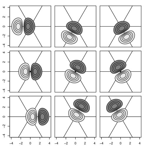
Figure 2: Synthesis of orientation-tuned subunits. The nine filters were synthesized from eight oriented derivatives centred at the origin (with of $\sigma=1$). The steered-additive solution of section 2.5.3 was used. Middle row: The $G_{1}$ filter is steered to the axes of a hexagonal lattice; $\theta=0^{\circ}\!,60^{\circ}\!,120^{\circ}$. Top and bottom rows: Offset filters, synthesized at shifts of $t=\pm\rho$ in the corresponding directions (with $\rho=1.5$). Note that each column can be interpreted as three subunits of an orientation-tuned complex cell. The filter amplitudes are scaled to the range $[-1,1]$, with contour lines separated by increments of 0.2 units.

2.4 Unconstrained Estimation

It will now be shown that the $K^{2}$ unknown coefficients, contained in the matrix $\mathitbf{C}$, can be obtained by standard least-squares methods. It should be emphasized that this is a filter-design problem; the matrix $\mathitbf{P}$ is fixed for all signals, and the response $\mathitbf{r}$ is obtained according to (16).

Let the $M\times N$ matrix $\mathitbf{F}_{\star}$ contain the true derivative filters, such that the $ij$-th element is $G_{1}(x_{j}-t_{i},\sigma)$. The approximation $\mathitbf{F}\approx\mathitbf{F}_{\star}$ can be expressed, according to (14 & 15), as the product

$$\mathitbf{F}_{\star}\approx\mathitbf{B}\mathitbf{C}\mathitbf{G},\quad\text{of which}\quad\mathitbf{C}=\mathitbf{B}^{+}\mathitbf{F}_{\star}\mathitbf{G}^{+}$$ (17)

is the solution in the least-squares sense. This formulation requires two Moore-Penrose inverses, which can be computed from the singular-value decompositions of the monomial basis and Gaussian derivative matrices $\mathitbf{B}$ and $\mathitbf{G}$, respectively. It is, however, more efficient to solve this problem using QR decompositions, as follows. There are, in practice, more offsets than derivative filters $M>K$, as well as more spatial samples than derivative filters $N>K$. The basis matrix has full column-rank $K$, and can be factored as $\mathitbf{B}=\mathitbf{Q}_{B}\mathitbf{R}_{B}$. The derivative matrix has full row-rank $K$, and so its transpose can be factored as $\mathitbf{G}^{\scriptscriptstyle\top}=\mathitbf{Q}_{G}\mathitbf{R}_{G}$. It follows that the solution (17) can be obtained via $\mathitbf{B}^{+}=\mathitbf{R}_{B}^{-1}\mathitbf{Q}_{B}^{\top}$ and $\mathitbf{G}^{+}=\mathitbf{Q}_{G}\mathitbf{R}_{G}^{-\!\top}$.

2.5 Constrained Estimation

The least-squares construction of the filters $\mathitbf{F}$ was described in the preceding section. The method is quite usable, but has two shortcomings. Firstly, if one of the shifts $t_{i}$ is zero, then $F(0,x)\approx G_{1}(x,\sigma)$, but it would be preferable to make this an exact equality, so that the original filter is returned as in (8). The second shortcoming of the method in 2.4 is that, in two or more dimensions, the orientation of the derivative filters in the basis-set $\mathitbf{G}$ may not match that of the target-set $\mathitbf{F}_{\star}$. Both of these problems will be solved below.

2.5.1 Additive Solution

The requirement $F(0,x)=G_{1}(x,\sigma)$ is satisfied by an additive model, in which the polynomial $P_{1}(t)$ that weights $G_{1}(x,\sigma)$ is always unity, and all other polynomials pass through zero when $t=0$. This implies the following partitioning of the derivative, monomial and coefficient matrices:

$$\mathitbf{G}=\begin{pmatrix}\mathitbf{g}_{1}^{\scriptscriptstyle\top}\\[3.22916pt] \mathitbf{G}_{\Delta}\end{pmatrix}\quad\mathitbf{B}=\begin{pmatrix}\mathitbf{1}\mspace{10.0mu}\mathitbf{B}_{\Delta}\end{pmatrix}\quad\mathitbf{C}=\begin{pmatrix}1&\mathitbf{0}^{\scriptscriptstyle\top}\\[2.15277pt] \mathitbf{0}&\mathitbf{C}_{\Delta}\end{pmatrix}$$ (18)

where $\mathitbf{1}$ is the column-vector of $M$ ones, and $\mathitbf{0}$ is the column-vector of $(K-1)$ zeros. The $1\times N$ vector $\mathitbf{g}_{1}^{\scriptscriptstyle\top}$ contains the first derivative filter $G_{1}(x,\sigma)$, while the $(K-1)\times N$ matrix $\mathitbf{G}_{\Delta}$ contains the higher-order filters. The columns of the $M\times(K-1)$ matrix $\mathitbf{B}_{\Delta}$ contain the sampled monomials, excluding the constant vector $\mathitbf{1}$. The unknown matrix $\mathitbf{C}$ will be recovered in the form indicated, where $\mathitbf{C}_{\Delta}$ has dimensions $(K-1)\times(K-1)$.

The product of $\mathitbf{B}$ and $\mathitbf{C}$, as in (14), now gives $\mathitbf{P}=(\mathitbf{1}\mspace{10.0mu}\mathitbf{P}_{\Delta})$, where the columns of $\mathitbf{P}_{\Delta}=\mathitbf{B}_{\Delta}\mathitbf{C}_{\Delta}$ are polynomials without constant terms. It follows that the product $\mathitbf{P}\mathitbf{G}$, as in (15), gives the additive approximation

$$\mathitbf{F}_{\star}\approx\mathitbf{1}\mathitbf{g}_{1}^{\scriptscriptstyle\top}+\mathitbf{B}_{\Delta}\mathitbf{C}_{\Delta}\mathitbf{G}_{\Delta}$$ (19)

where $\mathitbf{1}\mathitbf{g}_{1}^{\scriptscriptstyle\top}$ is the rank-one matrix containing $M$ identical rows $\mathitbf{g}_{1}^{\scriptscriptstyle\top}$. Note that if the $i$-th row of $\mathitbf{F}_{\star}$ corresponds to $t=0$, then the $i$-th row of $\mathitbf{B}_{\Delta}\mathitbf{C}_{\Delta}$ must be zero, this being the evaluation of the polynomials $\sum_{j=1}^{K-1}t^{j}c_{jk}$ at $t=0$. It follows that the $i$-th row of $\mathitbf{F}_{\star}$ is exactly recovered from (19) as $\mathitbf{g}_{1}^{\scriptscriptstyle\top}$, and so the constraint $F(0,x)=G_{1}(x,\sigma)$ has been imposed.

The unknown coefficients $\mathitbf{C}_{\Delta}$ are recovered by subtracting $\mathitbf{1}\mathitbf{g}_{1}^{\scriptscriptstyle\top}$ from $\mathitbf{F}_{\star}$, and then proceeding by analogy with (17). This leads to

$$\mathitbf{C}_{\Delta}=\mathitbf{B}_{\Delta}^{+}\bigl{(}\mathitbf{F}_{\star}-\mathitbf{1}\mathitbf{g}_{1}^{\scriptscriptstyle\top}\bigr{)}\mathitbf{G}_{\Delta}^{+}$$

where the matrices $\mathitbf{B}_{\Delta}^{+}$ and $\mathitbf{G}_{\Delta}^{+\!\top}$ can be obtained from the QR factorizations of $\mathitbf{B}_{\Delta}$ and $\mathitbf{G}_{\Delta}$, as before.

2.5.2 Steered Solution

In two (or more) dimensions, it is assumed that the desired filters $G_{1}(x-t,\theta,\sigma)$ have a common orientation, where $\mathitbf{v}=(\cos\theta,\sin\theta)^{\scriptscriptstyle\top}$ is the direction of the derivative in 2-d. This leads to invariance with respect to translations of the signal in the given direction. The basis filters $G_{k}(x,\sigma,\theta)$, however, will typically have a range of orientations $\phi_{\ell}\neq\theta$. This problem can be solved as follows.

Recall from section 2 that the $k$-th order Gaussian derivative is steerable with a basis of size $k+1$. Now suppose that row $k$ of the matrix $\mathitbf{G}$ is replaced by $k+1$ rows, containing sampled filters $G_{k}(x,\phi_{\ell},\sigma)$ at $\ell=1,\ldots,k+1$ distinct orientations $\phi_{\ell}$. The enlarged matrix $\mathitbf{G}_{\phi}$ now has dimensions $M_{K}\times N$, where

$$M_{K}=\sum_{k=1}^{K}(k+1)=\tfrac{1}{2}K(K+3).$$ (20)

It follows that there is a $K\times M_{K}$ ‘steering’ matrix $\mathitbf{D}$ such that $\mathitbf{G}=\mathitbf{D}\mathitbf{G}_{\phi}$ is exactly the $K\times N$ matrix of derivatives at the desired orientation. Moreover, if the approach of section 2.4 is applied to the $M_{K}\times N$ matrix $\mathitbf{G}_{\phi}$, then a solution

$$\mathitbf{F}=\mathitbf{B}\mathitbf{C}_{\phi}\mathitbf{G}_{\phi}=\mathitbf{B}\mathitbf{C}\mathitbf{G}$$ (21)

will be obtained. It follows that the two coefficient matrices are related by $\mathitbf{C}_{\phi}=\mathitbf{C}\mathitbf{D}$. In summary, if the matrix $\mathitbf{G}$ contains a sufficient number $M_{K}$ of differently oriented filters, then a set of translated filters $\mathitbf{F}$ can be approximated in any common orientation $\theta$. There is no change to the algorithm described in section 2.4. It should, however, be noted that (20) shows a trade-off between translation invariance and steerability. Larger translation invariance requires more derivatives, but these become increasingly difficult to steer.

2.5.3 Additive Steered Solution

The steered solution, as described in the previous section, will not automatically be additive, in the sense of (19). This problem will be solved, with reference to section 2.5.1, by putting an explicitly steered filter $\mathitbf{g}_{\theta}^{\scriptscriptstyle\top}$ in place of $\mathitbf{g}_{1}^{\scriptscriptstyle\top}$. The first derivative can be steered with respect to a basis of filters at distinct orientations $\phi_{1}$ and $\phi_{2}$ (these would be the first two rows of the $M_{K}\times N$ matrix $\mathitbf{G}_{\phi}$). The standard steering equation (Freeman and Adelson,, 1991) can be simplified in this case to

$$\begin{pmatrix}\cos\theta\\ \sin\theta\end{pmatrix}=\begin{pmatrix}\cos\phi_{1}&\cos\phi_{2}\\ \sin\phi_{1}&\sin\phi_{2}\end{pmatrix}\begin{pmatrix}p_{1}\\ p_{2}\end{pmatrix}$$

where $\theta$, $\phi_{1}$ and $\phi_{2}$ are known angles. This system can be solved exactly for the unknown coefficients $p_{1}$ and $p_{2}$, resulting in

$$\begin{gathered}p_{1}=\sin(\phi_{2}-\theta)/\delta\quad\text{and}\quad p_{2}=\sin(\theta-\phi_{1})/\delta\\ \quad\text{where}\quad\delta=\sin(\phi_{2}-\phi_{1}).\end{gathered}$$ (22)

It may be noted that if $\phi_{1}=0$ and $\phi_{2}=\pi/2$, then the solution reduces to the usual coefficients $p_{1}=\cos\theta$ and $p_{2}=\sin\theta$ for the construction of the directional derivative from $\mathrm{d}/\mathrm{d}x$ and $\mathrm{d}/\mathrm{d}y$. The additive steered approximation can now be defined, using the new filter $G_{1}(\mathitbf{x},\theta,\sigma)$, as

$$\mathitbf{F}_{\star}\approx\mathitbf{1}\mathitbf{g}_{\theta}^{\scriptscriptstyle\top}+\mathitbf{B}_{\Delta}\mathitbf{C}_{\phi\Delta}\mathitbf{G}_{\phi\Delta}\quad\text{where}\quad\mathitbf{g}_{\theta}^{\scriptscriptstyle\top}=p_{1}\mathitbf{g}_{\phi_{1}}^{\scriptscriptstyle\top}+p_{2}\mathitbf{g}_{\phi_{2}}^{\scriptscriptstyle\top}.$$ (23)

This system can be solved in the same way as (19). Note that the higher-order filters in $\mathitbf{G}_{\phi\Delta}$ will be implicitly steered, as described in section 2.5.2.

3 Evaluation

Two issues are addressed in this evaluation, as follows. Approximation: The accuracy of the least-squares algorithms from sections 2.4 and 2.5 is established in section 3.1. Characterization: The response of the underlying model from section 1.1 to basic stimuli, as well as to natural images, is analyzed in sections 3.2 and 3.3 respectively. Note that the issues of approximation and characterization are addressed separately, in order to avoid mixing different sources of error. Hence section 3.1 will evaluate the approximate filters $F$, while sections 3.2 and 3.3 will analyze the ideal filters $F_{\star}$.

3.1 Approximation Error

The accuracy of the filter approximations will be evaluated in this section, and it will be shown that the least-squares methods are superior to the original Maclaurin expansion. The evaluation is based on the root mean-square (RMS) error between the target and synthetic filters.

The accuracy of a given filter-synthesis method is determined by two variables; the range of offsets, and the number of available derivatives (size of the basis). Better approximations can, in general, be obtained by reducing the range of offsets and/or increasing the size of the basis. The range $\rho=1\sigma$ is the smallest that results in a unimodal impulse response, as will be shown in section 3.2.1. It is therefore important to analyze the corresponding approximation. In addition, the larger range $\rho=1.5\sigma$ will be analyzed. This leaves the size of the basis (for which there is no prior preference) to be varied in each case.

The method of evaluation is illustrated in figure 3. It can be seen that the furthest-offset filters begin to depart from the target shape. The RMS difference between the ideal and approximate filters, for each test, was measured over 51 offsets $t_{i}$ in the range $\pm\rho$. Each filter was sampled at 101 points $x_{j}$ in the range $\pm 6\sigma$, which contains the significantly nonzero part of all filters (see fig. 3).

The RMS error, for basis sizes $K=3,\ldots,10$ is shown in fig. 4. The meaning of the RMS error, in terms of filter distortion, can be gauged with reference to fig. 3. For example, it can be seen that the Maclaurin model with $K=8$ and $\rho=1.5$ is poor, and this corresponds to a point around the middle of the RMS axis in fig. 4.

In the case of the Maclaurin approximation (top row) it can be seen that the error increases rapidly and monotonically with respect to the offset. The pattern is more complicated for the least-squares approximations, because the error has been minimized over an interval $\pm\rho$, which effectively truncates the basis functions in $x$. Nonetheless, the lines corresponding to the different basis-sizes remain nested; they cannot cross, because increasing the size of the basis cannot make the approximation worse. It is, however, possible for the lines to meet. In particular, the unconstrained lines meet in pairs at $t=0$. This is because the target function at zero offset is anti-symmetric. It follows that the incorporation of a symmetric basis function $G_{2k}$ cannot improve an existing approximation of order $2k-1$. In the case of the additive approximation, all lines meet at $t=0$, where the error is zero by construction.

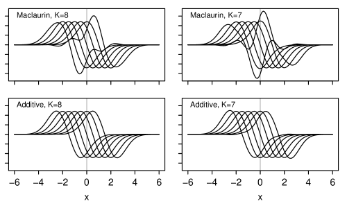
Figure 3: Filter deformation. Top left: The eighth-order Maclaurin synthesis (11) of filters $\sigma=1$, over a range $\rho=\pm 1.5\sigma$ of offsets. Large errors are visible in the most extreme filters. Top right: The approximation is much worse if the order of the basis is reduced by one. Bottom left, right: The least-squares approximation is much better, even if the additivity constraint is enforced.

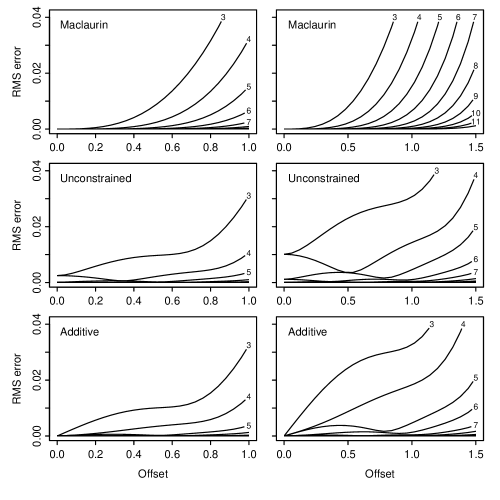
Figure 4: Error vs. offset. Top row: The Maclaurin error rises quickly as the target filter is offset from the centre of the basis. Each line represents a different basis-size, $k=3,\ldots,12$, as indicated. The left and right plots show ranges $\rho=1\sigma$, and $\rho=1.5\sigma$, respectively. Middle row: The unconstrained least-squares approximation is much better, especially for high-order bases. Bottom row: The additive approximation is also good, and ensures that the error is zero when there is no offset (as in the Maclaurin case).

3.2 Response to Basic Signals

A number of basic signals will be introduced below, and the ideal responses will be derived; further examples are given in Hansard and Horaud, (2010). The responses are ‘ideal’ in the sense that the error of the least-squares approximations (sec. 2.4–2.5.3) will be ignored. This is primarily in order to obtain useful results, but there are two further justifications. Firstly, it has been demonstrated in the preceding section that the approximations are good, over an appropriate range $\rho$. Secondly, the approximation error can be made arbitrarily low, by using a large enough basis for the given range.

Recall that the offset filters $F(t,x)$ are copies of the Gaussian derivative $G_{1}(x,\sigma)$. It follows from (9) that the response function is covariant to the shift $t$, in the sense that

$$R(t,u)=R(0,u-t).$$ (24)

It therefore suffices to obtain the linear response for the case $t=0$, as the other responses are simply translations of this function. The linear response in this case is $R(0,u)=G_{1}^{1}(x,\sigma)\star S(x-u)$, by analogy with (7). Note that the normalized filter has been used, as defined in (6). It follows that $R(0,u)$ can be obtained by blurring the signal with the filter $G_{0}^{1}(x,\sigma)$, and then differentiating the result. The complex response $C(u)$ is given by the max operation (10). Evidently $C(u)$ is the upper envelope of the family $|R(t,u)|$, but it is possible to be more precise than this. In particular, the shift-insensitivity of the model can be quantified by determining the intervals of $u$ over which $C(u)$ is constant, as described below.

The response $|R(0,u)|$ to a basic signal $S(x-u)$ can be either symmetric or antisymmetric, and either periodic or aperiodic. However, a common property of the responses considered here is that the local maxima are all of equal height. Let $|R(0,u^{\star})|=R^{\star}$ be a local maximum, and suppose that $u$ is within range of this maximum, meaning that $|u-u^{\star}|\leq\rho$. It follows that $C(u)=R^{\star}$, because the maximum in (10) will be found at $t=u-u^{\star}$, and $|R(u-u^{\star},u)|=|R(0,u^{\star})|=R^{\star}$ by (24). An intuitive summary of this is that each local maximum $|R(0,u^{\star})|$ generates a plateau $C(u^{\star}\pm\rho)=R^{\star}$ in the complex response. In order to make use of this interpretation, the function $V(u)$ will be defined as the signed distance $u-u^{\star}$ to the nearest local maximum of $|R(0,u)|$. It follows that

$$C(u)=\begin{cases}R^{\star}&\text{if}\mspace{10.0mu}|V(u)|\leq\rho\\ \underset{|t|\leq\rho}{\max}\mspace{5.0mu}|R(t,u)|&\text{otherwise}.\end{cases}$$ (25)

This explicitly identifies the intervals, $|V(u)|\leq\rho$, over which $C(u)$ is constant. Note that if $V(u)>\rho$ then the original definition (10) is used. The functions $R(0,u)$ and $V(u)$, as well as the constant $R^{\star}$, will now be derived for each of the basic signals. It should be emphasized that $V(u)$ and $R^{\star}$ are only used to characterize the response; they are not part of the computational model.

3.2.1 Impulse

The first test signal to be considered is the unit impulse, which can be used to characterize the initial linear stage of the model. The impulse is defined as

$$S_{\sigma}(x)=\delta(x)$$ (26)

where $\delta(x)$ is the Dirac distribution. It follows that the linear response $G_{1}^{1}\star S_{\sigma}$ is just the original normalized derivative filter,

$$R_{\sigma}(0,u)=G_{1}^{1}(u,\sigma).$$ (27)

The maxima of the linear response can be found by differentiating $R_{\sigma}(0,u)$, and setting the result to zero. The derivative contains a factor $\sigma^{2}-u^{2}$, and so the zeros are at $\pm\sigma$. The peak is at $-\sigma$, and it follows that the maximum response is

$$R^{\star}_{\sigma}=G_{1}^{1}(-\sigma,\sigma).$$ (28)

Both extrema become peaks in $|R_{\sigma}(0,u)|$, and the extent of the response plateau is determined by the minimum distance from these. The distance function for the impulse response can now be defined as

$$V_{\sigma}(u)=u-\mathrm{sgn}_{+}\mspace{-1.0mu}(u)\,\sigma,$$ (29)

where $\mathrm{sgn}_{+}$ is the sign-function with the convention $\mathrm{sgn}_{+}(0)=1$. If $u=0$ then $|V_{\sigma}(u)|=\sigma$, and it follows from (25) that $C(u)\neq R^{\star}_{\sigma}$ if $\sigma>\rho$. It has already been established that $|R_{\sigma}(0,u)|$ has maxima of $R^{\star}_{\sigma}$ at $\pm\sigma$, which implies that the response $C(u)$ will be bimodal unless

$$\sigma\leq\rho$$ (30)

as illustrated figure 5. This condition is strictly imposed, as it would be undesirable to have a bimodal response to a unimodal signal. In general, $\rho$ should be made as large as possible for a given $\sigma$, in order to achieve as much shift-invariance as possible. Recall, for example, that the least-squares approximations in section 3.1 were demonstrated for $\rho=1.5\sigma$.

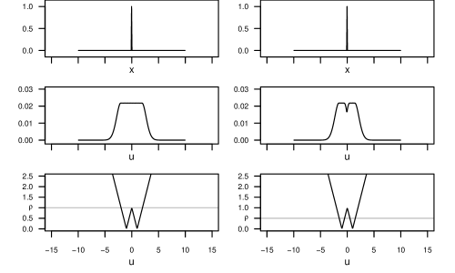
Figure 5: Impulse response. Left column: the top plot shows the unit impulse, $S_{\sigma}(x)$, as in (26). The middle plot shows the response $C(u)$. The bottom plot shows the distance function $|V_{\sigma}(u)|$, as in (29), along with the value of the maximum offset $\rho=1\sigma$. The response is constant, $C(u)=R^{\star}_{\sigma}$, when $|V_{\sigma}(u)|\leq\rho$. The critical case, $\sigma=1$, $\rho=1$ is plotted. Right column: as before, except $\rho=0.5\sigma$. The response becomes bimodal, which shows the importance of the condition $\sigma\leq\rho$.

3.2.2 Step

The second test signal to be considered is the unit step function. This is arguably the most important example, because it is the basic model for a luminance edge. Indeed, the current model is optimized for the detection of step-like edges, owing to the use of the first derivative as the offset filter (Canny,, 1986). The step can be defined from the standard sign-function, as follows

$$S_{\alpha}(x)=\frac{\alpha}{2}\bigl{(}1+\mathrm{sgn}(x)\bigr{)}$$ (31)

The unit step function is related to the integral $\varPhi(u,\sigma)$ of the normalized Gaussian function $G_{0}^{0}(x,\sigma)$ in the following way:

$$\mathit{\Phi}(u,\sigma) =\int_{-\infty}^{u}G^{0}_{0}(x,\sigma)\ \mathrm{d}x$$ (32)

$$=\frac{1/\alpha}{\sigma\sqrt{\pi/2}}\int_{-\infty}^{\infty}G^{1}_{0}(x,\sigma)\mspace{3.0mu}S_{\alpha}(u-x)\ \mathrm{d}x$$ (33)

The third integral is the convolution of $G_{0}^{1}$ with $S_{\alpha}$, and hence $\mathit{\Phi}(u,\sigma)$ is proportional to the smoothed step-edge. The linear response is given by the derivative,

$$R_{\alpha}(0,u) =\frac{\sigma\sqrt{\pi/2}}{1/\alpha}\,\frac{\mathrm{d}}{\mathrm{d}u}\,\varPhi(u,\sigma)$$ (34)

$$=\frac{\alpha}{2}\,G(u,\sigma)$$ (35)

This shows that the basic response is simply an un-normalized Gaussian, located at the step-discontinuity. The maximum response and the signed-distance function are evidently

$$R^{\star}_{\alpha}={\alpha}/{2}\quad\text{and}\quad V(u)=u.$$ (36)

Let $\bigl{(}u,R(u)\bigr{)}$ be the Cartesian coordinates of the response curve. The final response can be constructed from the Gaussian (35) by inserting the plateau $(\pm\rho,\alpha/2)$ in place of the maximum point $(0,\alpha/2)$. This is illustrated in in figure 6.

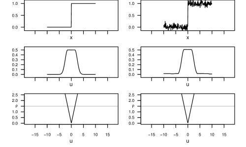
Figure 6: Step response. Left column: The top plot shows the step-edge $S_{\alpha}(x)$, as defined in (31). The middle plot shows the response $C(u)$. The bottom plot shows the distance function $V_{\alpha}(u)$, as in (36). Note that the response is unconditionally unimodal in this case. Right column: As before, except with Gaussian noise (SD 0.075) added independently at each point. The response $C(u)$ is not significantly affected.

3.2.3 Cosine

The third class of signals to be considered are the sines and cosines. These are of central importance, owing to their role in the Fourier synthesis of more complicated signals. Furthermore, these functions are used to construct the 2-d grating patterns that are commonly used to characterize complex cells. It will be convenient to base the analysis on the cosine function

$$S_{\xi}(x)=\cos\bigl{(}2\pi\xi x\bigr{)}$$ (37)

where $\xi$ is the frequency. The Fourier transforms $g(x)\mapsto\mathcal{F}_{x}[g](\eta)$ of the filter $G_{0}^{1}(x,\sigma)$ and signal $S_{\xi}(x)$ are

$$\mathcal{F}_{x}\bigl{[}G_{0}^{1}\bigr{]}(\eta) =\sigma\sqrt{\pi/2}\,G\bigl{(}\eta,1/(2\pi\sigma)\bigr{)}$$ (38)

$$\mathcal{F}_{x}\bigl{[}S_{\xi}\bigr{]}(\eta) =\tfrac{1}{2}\bigl{(}\delta(\eta-\xi)+\delta(\eta+\xi)\bigr{)}$$ (39)

respectively, where $\eta$ is the frequency variable. The convolution $G_{0}^{1}\star S_{\xi}$ can be obtained from the inverse Fourier transform of the product $\mathcal{F}_{x}\bigl{[}G_{0}^{1}]\,\mathcal{F}_{x}\bigl{[}S_{\xi}\bigr{]}$. The resulting cosine is attenuated by a scale-factor $\mathcal{F}_{x}\bigl{[}G_{0}^{1}\bigr{]}(\xi)$, because $\mathcal{F}_{x}\bigl{[}S_{\xi}](\eta)$ is zero unless $|\eta|=\xi$. Differentiating $\cos(2\pi\xi x)$ with respect to $x$ gives $-\sin(2\pi\xi x)$, along with a second scale-factor of $2\pi\xi$. The amplitude of the linear response is given by the product of the two scale-factors $2\pi\xi$ and $\mathcal{F}_{x}\bigl{[}G_{0}^{1}](\xi)$, which can be expressed as

$$R^{\star}_{\xi}=\sigma\xi\pi^{3/2}\sqrt{2}\,G\bigl{(}\xi,1/(2\pi\sigma)\bigr{)}.$$

It can be seen that the amplitude depends on the scale $\sigma$ of the filter, as well as on the frequency $\xi$ of the signal. The complete linear response is given by

$$R_{\xi}(0,u)=-R^{\star}_{\xi}\sin\bigl{(}2\pi\xi u\bigr{)}.$$

Note that a phase-shift $u_{0}$ can be introduced, if required, by substituting $u-u_{0}$ for $u$. The rectified sine $|R_{\xi}(0,u)|$ is another periodic function, of twice the frequency. The peaks of this function are separated by a distance $\frac{1}{2\xi}$, and so

$$V_{\xi}(u)=\biggl{(}u\bmod\frac{1}{2\xi}\biggr{)}-\frac{1}{4\xi}$$ (40)

is a suitable distance function for the cosine signal (37). The case of sine signals is analogous, with $\sin$ replaced by $\cos$ in the linear response (3.2.3), and $u$ replaced by $u-\frac{1}{4\xi}$ in the distance function (40).

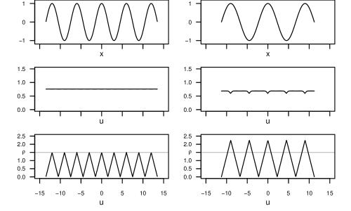
Figure 7: Cosine response. Left column: The top plot shows the cosine signal $S_{\xi}(x)$, as in (37), of frequency $\xi=\frac{1}{6}$. The middle plot shows the response $C(u)$, which is constant. The bottom plot shows the distance function $|V_{\xi}(u)|$, as in (40). Note that the critical case is plotted, in which the peaks of $|V_{\xi}(u)|$ touch the line $\rho=1.5\sigma$. The response is also constant for any higher frequency. Right column: As before, but for a lower frequency, $\xi=\frac{1}{9}$. The distance function now crosses the line $\rho=1.5\sigma$, and corresponding ‘notches’ appear in $C(u)$.

It is important to see that the system response is entirely constant for frequencies that are not too low. Specifically, the extreme values of (40), with respect to $u$, are $\pm\frac{1}{4\xi}$, from which it follows that the response is identically $R^{\star}_{\xi}$ if $\xi\geq\frac{1}{4\rho}$. The corresponding constraint on the wavelength $\frac{1}{\xi}$ is

$$1/\xi\leq 4\rho.$$ (41)

In order to interpret this result, recall that $\rho\geq\sigma$ is required for a unimodal impulse response (30). Furthermore, in section 3.1, it was shown that $\rho\approx 1.5\sigma$ is achievable in practice. This means that a constant response can be expected for frequencies as low as $\xi=\frac{1}{6\sigma}$.

3.3 Response to Natural Images

This section makes a basic evaluation of the differential model, using the objective function of ‘slow feature analysis’ (Wiskott and Sejnowski,, 2002; Berkes and Wiskott,, 2005). The procedure is as follows. Each $1024\times 768$ greyscale image is decomposed into $i=1,\ldots,36$ orientation channels $\theta_{i}$ at scale $\sigma=2$ pixels. This corresponds to a set of simple-cell responses $S_{1}(\mathitbf{x},\sigma,\theta_{i})$, with an angular separation of $5^{\circ}$. The steerability of $S_{1}$ is not used (i.e. a separate convolution is done for each $\theta_{i}$) in order to minimize any angular bias in the image sampling. A set of straight tracks

$$\mathitbf{x}_{ijk}=\mathitbf{p}_{j}\pm k\Delta\times(\cos\theta_{i},\,\sin\theta_{i})^{\scriptscriptstyle\top},\quad\text{where}\quad j=1,\ldots,m\quad\text{and}\quad k=0,\ldots,n$$ (42)

is sampled from each 2-d response. The $m=100$ random points $\mathitbf{p}_{j}$ are sampled from a uniform distribution over the image; the sign $\pm$ is also random. The resolution $\Delta$ is set to one pixel, and the number of steps along each path is $n=99$. This gives a total of $100^{2}$ samples from each orientation channel. The responses at non-integral positions $\mathitbf{x}_{ijk}$ are obtained by bilinear interpolation. The samples are non-negative by definition, and a global scale factor $\gamma$ is used to make the overall $ijk$-mean of $\gamma S_{1}(\mathitbf{x}_{ijk},\sigma,\theta_{i})$ equal to $\frac{1}{2}$. The mean simple-cell response is then computed in each orientation channel,

$$E_{S}(i)=\frac{1}{mn}\sum_{j=1}^{m}\sum_{k=0}^{n}\,\gamma S_{1}\bigl{(}\mathitbf{x}_{ijk},\sigma,\theta_{i}\bigr{)}$$ (43)

where the scaling by $\gamma$ ensures that $\sum_{i}E_{S}(i)=\frac{1}{2}$. The mean quadratic variation along the paths is also computed, in each orientation channel;

$$Q_{S}(i)=\frac{1}{mn}\sum_{j=1}^{m}\sum_{k=1}^{n}\,\Bigl{|}\gamma S_{1}\bigl{(}\mathitbf{x}_{ijk},\sigma,\theta_{i}\bigr{)}-\gamma S_{1}\bigl{(}\mathitbf{x}_{ij[k-1]},\sigma,\theta_{i}\bigr{)}\Bigr{|}^{2}.$$ (44)

The coordinates $\mathitbf{x}_{ijk}$ and $\mathitbf{x}_{ij[k-1]}$ represent adjacent points (separated by $\Delta$) on the $j$-th path in the $i$-th channel. In summary, $E_{S}(i)$ measures the average response for orientation $\theta_{i}$, and $Q_{S}(i)$ measures the average spatial variation of this response in direction $\theta_{i}$. Slow feature analysis finds filters that minimize the quadratic variation. The orientation tuning and slowness measurements are plotted in figures 8 and 9 as a function of $\theta_{i}$, by attaching vertical bars $\pm\frac{1}{2}\sqrt{Q_{S}(i)}$ to each point $E_{i}$. Each test is then repeated, using the complex response $C(\mathitbf{x},\sigma,\theta)$ in place of the simple response $S_{1}(\mathitbf{x},\sigma,\theta)$, giving measurements $E_{C}(i)$ and $Q_{C}(i)$.

Three test-images with a dominant global orientation are used. Firstly, a vertical cosine grating, $I_{\cos}(x,y)=\frac{1}{2}\bigl{(}1+\cos(2\pi\xi x)\bigr{)}$. The range is set to $\rho=1.5\sigma$, as usual, and the wavelength is set to $\frac{1}{\xi}=8\sigma$. These values do not satisfy the limit (41), which ensures that the complex response will not be trivial. The simple-cell response is shown in figure 8 (top left), and two effects should be noted. Firstly, the response is tuned to the dominant orientation $\theta=0$, as can be seen from the unimodal shape of the curve. Secondly, there is a large variation in the response when the tracks are orthogonal to the grating, as shown by the large bars around $\theta=0$. This is because the filter falls in and out of phase with the image as it moves horizontally. The corresponding complex response is shown in figure 8 (top right). It can be seen that the orientation tuning is preserved, while the response variation is greatly reduced. Figure 8 (bottom) repeats the test, but with noise added to the cosine grating, $I=0.25\times I_{\cos}+0.75\times I_{\mathrm{uni}}$, where each pixel in $I_{\mathrm{uni}}$ is independently sampled from the uniform distribution on $[0,1]$. This means that a variable simple response is obtained as the filter moves in any direction, because the image is now truly 2-d. The complex response reduces the variation, as shown in figure 8 (bottom).

Figure 9 (top) shows results for a real image which has an orientation-structure similar to that of the grating. The results are analogous. Finally, the same test is performed on a natural image, which contains a mixture of foliage and rocks. Figure 9 (bottom) shows that, although there is no dominant orientation in the stimulus, the complex response remains much less variable than the simple response.

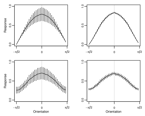
Figure 8: Cosine response. Top left: Average simple cell response $E_{S}(i)$ to a vertical cosine grating of wavelength $8\sigma$. The curve indicates the mean response in each of 36 orientation channels $\theta_{i}$, and has a clear peak at zero. The vertical bars $\pm\frac{1}{2}\sqrt{Q_{S}(i)}$ indicate the rms spatial variation of the response in the preferred direction of each orientation channel. Top right: Complex cell response $E_{C}(i)$ to the same image. The orientation tuning is preserved, but the variability $\pm\frac{1}{2}\sqrt{Q_{C}(i)}$ of the response is greatly reduced. Bottom left, right: As before, but with noise added to the image.

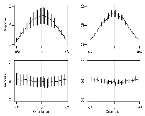
Figure 9: Image response. Top: As in figure 8, but using a real image that contains a dominant vertical orientation. Left: The simple response shows variation across all orientation channels $Q_{S}(i)$. Right: The variation of the complex response $Q_{C}(i)$ is much lower. Bottom: As before, but using a natural image, with no dominant orientation.

4 Discussion

It has been shown that a differential model of the complex cell can be constructed from the local jet representation. The differential model, which works naturally in a basis of steerable filters, can be viewed as a constrained version of the Hubel and Wiesel, (1962) subunit model.

4.1 Neural Implementation

The qualitative components in the present approach are similar to those of the Gabor energy model. Both models are based on oriented linear filters, which are centred at the same position. Likewise, both models output a combination of the nonlinearly transformed filter responses. The derivative operators $G_{k}(x,\sigma)$, in the differential model, are interpreted as simple cells, at a common location $x$ (Hawken and Parker,, 1987; Young et al.,, 2001). These are constructed from LGN inputs, according to the classical model (Hubel and Wiesel,, 1962). The offset filters $F(t_{i},x)$ have two possible interpretations, shown in fig. 10, as follows.

Firstly, the offset filters $F(t_{i},x)$ can be interpreted as an intermediate layer of simple cells, each of which has an RF that is a linear combination of other simple cell RFs. Let the row-vector $\mathitbf{f}_{i}^{\scriptscriptstyle\top}$ represent $F(t_{i},x)$, and let $\mathitbf{s}$ be the signal vector. It follows that the linear response is

$$r_{i}=\mathitbf{f}_{i}^{\scriptscriptstyle\top}\!\mathitbf{s}$$ (45)

where $\mathitbf{f}_{i}^{\scriptscriptstyle\top}=\mathitbf{p}_{i}^{\scriptscriptstyle\top}\!\mathitbf{G}$, according to the filter-design equation $\mathitbf{F}=\mathitbf{P}\mathitbf{G}$ in (15). The task of the complex cell $C$ is to compute the (absolute) maximum of the linear responses, $r_{i}$. This interpretation corresponds to the hmax model (Riesenhuber and Poggio,, 1999; Lampl et al.,, 2004), but with additional relationships imposed on the underlying simple cells. An advantage of this interpretation is that it predicts a majority of simple cells with few oscillations, as is observed (Ringach,, 2002). This follows from the fact that the offset filters are of lower order than their derivatives, together with the fact that an unlimited number of offsets can be obtained from a given derivative basis. Furthermore, suppose that a number of complex cells (e.g. of different orientations) $C_{n}$ are constructed from the same basis $\mathitbf{G}$. A new layer of low-order offset filters $\mathitbf{F}_{n}$ is required for each complex cell, and so the high-order filters in $\mathitbf{G}$ are soon outnumbered in the ensemble $\{\mathitbf{G},\mathitbf{F}_{1},\mathitbf{F}_{2},\ldots\}$.

An alternative physiological implementation is as follows. Suppose that the complex cell has $i=1\ldots,M$ basal dendrites, each of which branches out to the $K$ simple cells $G_{k}(x,\sigma)$. The linear response can then be expressed as

$$r_{i}=\mathitbf{p}_{i}^{\scriptscriptstyle\top}(\mathitbf{G}\mathitbf{s})$$ (46)

where $\mathitbf{G}\mathitbf{s}$, the Gaussian jet response, is computed first. This interpretation requires no intermediate simple cells. Instead, it places a fixed weight $P_{ik}$ on each dendritic branch, and requires a summation to be performed within each dendrite. This seems to be quite compatible with the observed cell morphology; a typical complex cell has a small number of basal dendrites which, unlike those of simple cells, are extensively branched (Kelly and van Essen,, 1974; Gilbert and Wiesel,, 1979).

The dendritic interpretation is more economical in the number of simple cells required, but less compatible with the observed simple-cell statistics (Ringach,, 2002). It should be noted that a mixture of the two interpretations in fig. 10 is quite possible. For example, there could be a few intermediate simple cells, with the remaining filters implemented by dendritic summation. In all cases, each complex cell is associated with odd and even simple cells $\mathitbf{g}_{k}$, as is observed (Pollen and Ronner,, 1981).

Figure 10: Two neural implementations of the complex cell $C$. These are schematic representations, with reduced numbers of derivative filters $\mathitbf{g}_{k}$ and offset filters $\mathitbf{f}_{i}$. Left: The offset filters are identified with an intermediate layer of simple cells. Right: The offset filters are implicit in the weighted sums $\mathitbf{p}_{1}^{\scriptscriptstyle\top}\!\mathitbf{G}$ and $\mathitbf{p}_{2}^{\scriptscriptstyle\top}\!\mathitbf{G}$ performed by the dendritic tree of $C$.

The maximum (10) over the $|r_{i}|$ can be approximated by a barycentric combination, $\sum_{i}w_{i}|r_{i}|$. An appropriate vector of weights can be computed as $w_{i}=\mbox{$|r_{i}|^{\beta}\!\big{/}(\alpha+\sum_{i}|r_{i}|^{\beta})$}$. This is a form of ‘softmax’ (Bridle,, 1989), with parameters $\alpha$ and $\beta$, as described in (Hansard and Horaud,, 2010). Several neural models of this operation have been proposed (Riesenhuber and Poggio,, 1999; Yu et al.,, 2002). For example, the $w_{i}$ can be interpreted as the outputs of a network of mutually inhibitory neurons, which receive copies of the subunit responses $r_{i}$. There is experimental evidence for similar arrangements, with respect to both simple and complex cells (Heeger, 1992a, ; Carandini and Heeger,, 1994; Lampl et al.,, 2004).

4.2 Experimental Predictions

This section will demonstrate that the response of the new model, to broad-band stimuli, can easily be distinguished from that of the standard energy model. Some qualitative predictions will also be discussed.

The response of the new model to sinusoidal stimuli is similar to that of the energy model. Both responses are phase-invariant, provided that the stimulus frequency is not too low (see fig. 7). Consider, however, a luminance step-edge that is flashed (or shifted) across the RF. The Gabor energy is approximately Gaussian, as a function of the edge-position, with a peak in the centre of the RF. The differential response is much flatter, as shown in fig. 6. This suggests that an empirical measure of kurtosis could be used to distinguish between the two responses, as will be shown below.

Let the odd-symmetric Gabor filter be defined as $F_{\parallel}(x,\xi,\tau)=-G(x,\tau)\sin(2\pi\xi x)$, so that it matches the polarity of $G_{1}$. The even filter, following (Lehky et al.,, 2005), is defined by the numerical Hilbert transform $F_{\!\perp}=\mathcal{H}(F_{\parallel})$, in order to avoid the nonzero DC component that arises in the cosine-based definition. The Gabor energy of a signal $S$ is then $R_{F}^{2}=(F_{\parallel}\star S)^{2}+(F_{\!\perp}\star S)^{2}$. The envelope width $\tau$ of each Gabor filter is determined from the constraint that the bandwidth be equal to 1.5, which is realistic for complex cells (Daugman,, 1985). A self-similar family of Gabor pairs, parameterized by frequency $\xi$, can now be defined. Quasi-Newton optimization is used to determine a frequency $\xi_{0}$, for which $F_{\parallel}(x,\xi_{0},\tau)\approx G_{1}(x,1)$ in the $L^{2}$ sense. Ten Gabor pairs with frequencies $\xi_{k}=\xi_{0}2^{-k\Delta\xi}$ are constructed, where $k=0,\ldots 9$. The corresponding differential model, with target filter $G_{1}(x,\xi_{0}/\xi_{k})$, is also constructed for each pair. Four possible ranges are considered for the differential models, by setting $\rho/\sigma=1.0$, 1.25, 1.5, 1.75.

Let $p_{\xi}(u)$ be the response distribution, which gives the firing-rate for an image-edge, as a function of its offset $u$ from the centre $u=0$ of the complex RF. If $P_{\xi}(u)$ is the cumulative distribution $\int p_{\xi}(u)\,\mathrm{d}u$, then the (uncentred) kurtosis $\kappa$ of any $p_{\xi}(u)$ can be estimated (Crow and Siddiqui,, 1967) by

$$K(p_{\xi})=\frac{P_{\xi}^{-1}(1-a)-P_{\xi}^{-1}(a)}{P_{\xi}^{-1}(1-b)-P_{\xi}^{-1}(b)}.$$ (47)

The values $a=0.025$ and $b=0.25$ are used here (making $K$ the ratio of the 95% and 50% confidence intervals). This estimate, which can be computed by linear-interpolation between the samples of $P_{\xi}(u)$, has the following interpretation. Suppose that the offsets $u_{a}$ and $u_{b}$ are associated with firing-rates $a$ and $b$ respectively. The response distributions are symmetric, and so the statistic (47) is simply the distance ratio $K(p_{\xi})=u_{a}/u_{b}$, as illustrated in fig. 11. The kurtosis could also be estimated from the empirical moments of $p_{\xi}(u)$, but (47) is much less sensitive to noise in the tails of the distribution.

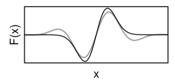
Figure 11: Top Left: Gaussian Derivative (black) and Gabor (grey) filters, matched subject to the bandwidth condition. Bottom Left: The kurtosis statistic (47) is the ratio of the two horizontal lines, shown here on a Gaussian distribution. Right: Kurtosis of the edge-response. Each line represents a complex cell model, parameterized by preferred frequency $\xi$. The top pair is obtained from the Gabor energy and its square-root. The bottom pair delimits the range of possible differential models. The Gabor and differential responses are easily distinguished. The dashed lines are estimates for reference distributions.

The distributions considered here lie in and around the range from the uniform distribution ($\kappa=\frac{9}{5}$, $K=1.9$), to the normal distribution ($\kappa=3$, $K\approx 2.91$). It can be seen from fig. 11 that the Gabor response is approximately Gaussian, whereas the differential responses are much flatter. Furthermore, note that the line $\rho=\sigma$ in fig. 11 shows the maximum kurtosis of the differential model (determined by 30), which is still much lower than that of the Gabor energy. Furthermore, it can be seen that the kurtosis is approximately independent of frequency, which simplifies the comparision. It should be noted that a much better fit between $G_{1}$ and $F_{\parallel}$ can be obtained if the bandwidth constraint is relaxed. This however, makes the energy responses even more kurtotic.

The differential model makes several predictions about the configuration of simple and complex cells. Firstly, like the energy model, it predicts that both odd and even filters are required by the complex cell. Unlike the energy model, it does not require an exact quadrature relationship (indeed, the $G_{k}$ basis is not orthogonal). More generally, an important property of the differential model is its robustness to deviations from the ideal simple-cell RF profiles. Derivative of Gaussian basis was used, in the present derivation, for mathematical clarity. However, all that is required is a basis that spans the space of desired subunit filters $F(t_{i},x)$.

The differential model also predicts a relationship between the scale $\sigma$ of the subunits and the radius $\rho$ of the resulting complex receptive field. This prediction, as in the case of the energy model, is probably too strict (i.e. larger complex receptive fields should be possible). However, as discussed in the following section, the complex receptive fields can be extended by allowing multiple scales $\sigma_{j}$ in the basis set of the differential model.

A qualitative prediction of the present model is that high-order derivative filters are required, in order to approximate the target filter over a sufficient range $\rho$. In particular, it was shown in section 3.2.1 that, for a unimodal impulse response, $\rho\geq\sigma$ is required. This means, in practice, that derivative filters of order five and beyond must be used in the approximation, as can be seen from figure 4. This is interesting, because very oscillatory filters have been observed in V1 (Young and Lesperance,, 2001). These have a natural role as high-frequency processors in the Gabor model. Their role is less clear in the geometric approach, because estimates of the high-order image derivatives are of limited use. The present work suggests that these filters could have a different role, in providing a basis for spatially offset filters of low order.

4.3 Future Directions

There are several directions in which this model could be developed. One straightforward extension is to allow filters of different scales (as well as different orders) in the basis set. Preliminary experiments confirm that this extends the range $\rho$ of translation invariance, as would be expected. This means that the complex cell receptive field could be made larger, relative to those of the underlying simple cells. Another extension would be to allow a variety of offset-filter shapes (with odd, even & mixed symmetry), rather than just the first derivative used here. This would lead to better agreement with the physiological data, which indicates a variety of receptive field shapes among the complex subunits (Gaska et al.,, 1987; Touryan et al.,, 2005; Sasaki and Ohzawa,, 2007). It would also be interesting to explore the relationship of the present work to the normalization model (Heeger, 1992b, ; Rust et al.,, 2005), and to other models of motion and spatial processing (Johnston et al.,, 1992; Georgeson et al.,, 2007).

The present work has concentrated on local shift-invariance, because this is a defining characteristic of complex cells. However, mechanisms that have other geometric invariances can be constructed in the same scale space framework. For example, consider the effect of a geometric scaling $(x,y)\rightarrow(\alpha x,\alpha y)$ on the operator $G_{0}^{0}(x,y,\sigma,\theta)$, which represents the $k$-th derivative of the normalized 2-d Gaussian, in direction $\theta$. The scaling $\alpha$ has no effect on the shape of the RF, as can be seen from the equation $G_{k}^{0}(\alpha x,\alpha y,\alpha\sigma,\theta)=G_{k}^{0}(x,y,\sigma,\theta)\big{/}\alpha^{2+k}$. This leads to simple relationships between the responses of the RF family $G_{k}^{0}(x,y,\sigma_{\ell},\theta)$, where $\ell=1,\ldots L$ defines a range of scales (Koenderink and van Doorn,, 1992; Lindeberg,, 1998). Future work will consider more complicated geometric invariances (e.g. 2-d affine), in connection with the larger RFs that are found in extrastriate areas.

Another direction would be to consider how the differential model could be learned from natural image data, by analogy with (Wiskott and Sejnowski,, 2002; Berkes and Wiskott,, 2005; Karklin and Lewicki,, 2009). This could be done by fixing the local jet filters (i.e. simple cells), and then optimizing the linear transformation $\mathitbf{P}$. The transformation could be parameterized by coefficients $\mathitbf{C}$, given a basis $\mathitbf{B}$ of smooth functions (e.g. the polynomials that were used here). Alternatively, $\mathitbf{P}$ could be optimized directly, subject to smoothness constraints on the columns $P_{k}(t)$. The variability of the response $C(u)$ would be a suitable objective function for the learning process, by analogy with slow-feature analysis models (Wiskott and Sejnowski,, 2002; Berkes and Wiskott,, 2005). The combination of the geometric and statistical approaches to image analysis is, more generally, a very promising aim.

References

- Adelson and Bergen, (1985) Adelson, E. H. and Bergen, J. R. (1985). Spatiotemporal energy models for the perception of motion. J. Opt. Soc. Am. A, 2(2):284–299.
- Alonso and Martinez, (1998) Alonso, J.-M. and Martinez, L. M. (1998). Functional connectivity between simple cells and complex cells in cat striate cortex. Nature Neuroscience, 1(5):395–403.
- Atherton, (2002) Atherton, T. J. (2002). Energy and phase orientation mechanisms: A computational model. Spatial Vision, 15(4):415–441.
- Ben-Shahar and Zucker, (2004) Ben-Shahar, O. and Zucker, S. W. (2004). Geometrical Computations Explain Projection Patterns of Long Range Horizontal Connections in Visual Cortex. Neural Computation, 16(3):445–476.
- Berkes and Wiskott, (2005) Berkes, P. and Wiskott, L. (2005). Slow feature analysis yields a rich repertoire of complex cell properties. Journal of Vision, 5(6):579–602.
- Bridle, (1989) Bridle, J. S. (1989). Probabilistic interpretation of feedforward classification network outputs, with relationships to statistical pattern recognition. In Fougelman-Soulie, F. and Hérault, J., editors, Neuro-computing: Algorithms, Architectures and Applictions. Springer Verlag.
- Canny, (1986) Canny, J. (1986). A computational approach to edge detection. IEEE Transactions on Pattern Analysis and Machine Intelligence, 8(6):679–698.
- Carandini, (2006) Carandini, M. (2006). What simple and complex cells compute. J. Physiology, 577(2):463–466.
- Carandini et al., (2005) Carandini, M., Demb, J. B., Mante, V., Tolhurst, D. J., Dan, Y., Olshausen, B. A., Gallant, J. L., and Rust, N. (2005). Do we know what the early visual system does? J. Neuroscience, 25:10577–10597.
- Carandini and Heeger, (1994) Carandini, M. and Heeger, D. (1994). Summation and Division by Neurons in Primate Visual Cortex. Science, 264:1333–1336.
- Crow and Siddiqui, (1967) Crow, E. and Siddiqui, M. (1967). Robust Estimation of Location. Journal of the American Statistical Association, 62(318):353–389.
- Daugman, (1985) Daugman, J. G. (1985). Uncertainty relation for resolution in space, spatial frequency, and orientation optimized by two-dimensional visual cortical filters. J. Optical Soc. America, 2(7):1160–1169.
- Dayan and Abbott, (2001) Dayan, P. and Abbott, L. F. (2001). Theoretical Neuroscience. MIT Press.
- Dobbins et al., (1987) Dobbins, A., Zucker, S. W., and Cynader, M. S. (1987). Endstopped neurons in the visual cortex as a substrate for calculating curvature. Nature, 329:438–441.
- Emerson et al., (1992) Emerson, R. C., Bergen, J. R., and Adelson, E. H. (1992). Directionally Selective Complex Cells and the Computation of Motion Energy in Cat Visual Cortex. Vision Research, 32(2):203–218.
- Felsberg and Sommer, (2001) Felsberg, M. and Sommer, G. (2001). The Monogenic Signal. IEEE Transactions on Signal Processing, 49(12):3136–3144.
- Fleet et al., (1996) Fleet, D. J., Wagner, H., and Heeger, D. J. (1996). Neural encoding of binocular disparity: Energy models, position shifts and phase shifts. Vision Research, 36(12):1839–1857.
- Freeman and Adelson, (1991) Freeman, W. T. and Adelson, E. H. (1991). The design and use of steerable filters. IEEE Trans. PAMI, 13(9):891–906.
- Gaska et al., (1987) Gaska, J. P., Pollen, D. A., and Cavanagh, P. (1987). Diversity of complex cell responses to even- and odd-symmetric luminance profiles in the visual cortex of the cat. Experimental Brain Research, 68:249–259.
- Georgeson et al., (2007) Georgeson, M. A., May, K. A., Freeman, T. C. A., and Hesse, G. S. (2007). From filters to features: Scale–space analysis of edge and blur coding in human vision. Journal of Vision, 7(13):1–21.
- Gilbert and Wiesel, (1979) Gilbert, C. and Wiesel, T. (1979). Morphology and Intracortical Projections of Fucntionally Characterised Neurones in the Cat Visual Cortex. Nature, 280(5718):120–125.
- Hansard and Horaud, (2010) Hansard, M. and Horaud, R. (2010). Complex Cells and the Representation of Local Image-Structure. Technical Report 7485, INRIA.
- Harris and Stephens, (1988) Harris, C. and Stephens, M. (1988). A combined corner and edge detector. In Proc. 4th Alvey Vision Conference, pages 147–151.
- Hawken and Parker, (1987) Hawken, M. J. and Parker, A. J. (1987). Spatial properties of neurons in the monkey striate cortex. Proc. R. Soc. Lond. B, B 231:251–288.
- (25) Heeger, D. J. (1992a). Half-Squaring in responses of cat striate cells. Visual Neuroscience, 9:427–443.
- (26) Heeger, D. J. (1992b). Normalization of Cell Responses in Cat Striate Cortex. Visual Neuroscience, 9:181–197.
- Hubel and Wiesel, (1962) Hubel, D. H. and Wiesel, T. N. (1962). Receptive fields, binocular interaction and functional architecture in the cat’s visual cortex. J. Physiology, 160:106–54.
- Johnston et al., (1992) Johnston, A., McOwan, P. W., and Buxton, H. (1992). A computational model of the analysis of some first-order and second-order motion patterns by simple and complex cells. Proc. R. Soc. Lond. B, 250:297–306.
- Jones and Palmer, (1987) Jones, J. P. and Palmer, L. A. (1987). An evaluation of the two-dimensional Gabor filter model of simple receptive fields in cat striate cortex. J. Neurophysiology, 58(6):1233–1258.
- Karklin and Lewicki, (2009) Karklin, Y. and Lewicki, M. S. (2009). Emergence of complex cell properties by learning to generalize in natural scenes. Nature, 457:83–86.
- Kelly and van Essen, (1974) Kelly, J. and van Essen, D. (1974). Cell Structure and Function in the Visual Cortex of the Cat. J. Physiology, 238:515–547.
- Kjaer et al., (1997) Kjaer, T. W., Gawne, T. J., Hertz, J. A., and Richmond, B. J. (1997). Insensitivity of V1 Complex Cell Responses to Small Shifts in the Retinal Image of Complex Patterns. J. Neurophysiology, 78:3187–3197.
- Koenderink and van Doorn, (1992) Koenderink, J. and van Doorn, A. (1992). Generic Neighborhood Operators. IEEE Transactions on Pattern Analysis and Machine Intelligence, 14(6):597–605.
- Koenderink, (1984) Koenderink, J. J. (1984). The structure of images. Biological Cybernetics, 50:363–370.
- Koenderink and van Doorn, (1987) Koenderink, J. J. and van Doorn, A. J. (1987). Representation of local geometry in the visual system. Biological Cybernetics, 55:367–375.
- Koenderink and van Doorn, (1990) Koenderink, J. J. and van Doorn, A. J. (1990). Receptive field families. Biological Cybernetics, 63:291–297.
- Lampl et al., (2004) Lampl, I., Ferster, D., Poggio, T., and Riesenhuber, M. (2004). Intracellular Measurements of Spatial Integration and the MAX Operation in Complex Cells of the Cat Primary Visual Cortex. J. Neurophysiology, 92:2704–2713.
- Lehky et al., (2005) Lehky, S. R., Sejnowski, T. J., and Desimone, R. (2005). Selectivity and sparseness in the responses of striate complex cells. Vision Research, 45:57–73.
- Lindeberg, (1998) Lindeberg, T. (1998). Edge Detection and Ridge Detection with Automatic Scale Selection. International Journal of Computer Vision, 30(2):117–154.
- Martinez and Alonso, (2003) Martinez, L. M. and Alonso, J.-M. (2003). Complex Receptive Fields in Primary Visual Cortex. The Neuroscientist, 9(5):317–331.
- De Valois et al., (1982) De Valois, R. L., Albrecht, D. G., and Thorell, L. G. (1982). Spatial frequency selectivity of cells in macaque visual cortex. Vision Research, 21:545–559.
- Mechler et al., (2002) Mechler, F., Reich, D. S., and Victor, J. D. (2002). Detection and Discrimination of Relative Spatial Phase by V1 Neurons. J. Neuroscience, 22(14):6129–6157.
- Mechler and Ringach, (2002) Mechler, F. and Ringach, D. L. (2002). On the Classification of Simple and Complex Cells. Vision Research, 42:1017–1013.
- Morrone and Burr, (1988) Morrone, M. and Burr, D. (1988). Feature detection in human vision: A phase dependent energy model. Proc. R. Soc. Lond. B., 235:221–245.
- (45) Movshon, J. A., Thompson, I. D., and Tolhurst, D. J. (1978a). Receptive field organization of complex cells in the cat’s striate cortex. J. Physiology, 283:79–99.
- (46) Movshon, J. A., Thompson, I. D., and Tolhurst, D. J. (1978b). Spatial summation in the receptive fields of simple cells in the cat’s striate cortex. J. Physiology, 283:53–77.
- Orban, (2008) Orban, G. A. (2008). Higher order visual processing in macaque extrastriate cortex. Physiological Reviews, 88:59–89.
- Perona, (1995) Perona, P. (1995). Deformable kernels for early vision. IEEE Trans. PAMI, 17(5):488–499.
- Petitot, (2003) Petitot, J. (2003). The Neurogeometry of Pinwheels as a Sub-Riemannian Contact Structure. J. Physiol Paris, 97:265–309.
- Pollen and Ronner, (1983) Pollen, A. D. and Ronner, S. F. (1983). Visual cortical neurons as localized spatial frequency filters. IEEE Transactions on Systems, Man & Cybernetics, 13:907–916.
- Pollen and Ronner, (1981) Pollen, D. A. and Ronner, S. F. (1981). Phase relationships between adjacent simple cells in the visual cortex. Science, 212(4501):1409–1411.
- Press et al., (1992) Press, W. H., Teukolsky, S. A., Vetterling, W. T., and Flannery, B. P. (1992). Numerical Recipes in C. Cambridge University Press, 2nd edition.
- Riesenhuber and Poggio, (1999) Riesenhuber, M. and Poggio, T. (1999). Hierarchical models of object recognition in cortex. Nature Neuroscience, 2(11):1019–1025.
- Ringach, (2002) Ringach, D. (2002). Spatial Structure and Symmetry of Simple-Cell Receptive Fields in Macaque Primary Visual Cortex. J. Neurophysiology, 88:455–463.
- Rust et al., (2005) Rust, N., Schwartz, O., Movshon, J., and Simoncelli, E. (2005). Spatiotemporal Elements of Macaque V1 Receptive Fields. Neuron, 46:945–956.
- Sasaki and Ohzawa, (2007) Sasaki, K. S. and Ohzawa, I. (2007). Internal Spatial Organization of Receptive Fields of Complex Cells in the Early Visual Cortex. J. Neurophysiology, 98:1194–1212.
- Simoncelli et al., (1992) Simoncelli, E. P., Freeman, W. T., Adelson, E. H., and Heeger, D. J. (1992). Shiftable Multiscale Transforms. IEEE Transactions on Information Theory, 38(2):587–607.
- Skottun et al., (1991) Skottun, B. C., Valois, R. L. D., Grosof, D. H., Movshon, J. A., Albrecht, D. G., and Bonds, A. B. (1991). Classifying Simple and Complex Cells on the basis of Response Modulation. Vision Research, 31(7/8):1079–1086.
- Spitzer and Hochstein, (1988) Spitzer, H. and Hochstein, S. (1988). Complex cell receptive field models. Progress in Neurobiology, 31:285–309.
- Touryan et al., (2005) Touryan, J., Felsen, G., and Dan, Y. (2005). Spatial Structure of Complex Cell Receptive Fields Measured with Natural Images. Neuron, 45:781–791.
- Wiskott and Sejnowski, (2002) Wiskott, L. and Sejnowski, T. (2002). Slow feature analysis: unsupervised learning of invariances. Neural Computation, 14(4):715–770.
- Wundrich et al., (2004) Wundrich, I. J., von der Malsburg, C., and Würtz, R. P. (2004). Image Representation by Complex Cell Responses. Neural Computation, 16(4):2563–2575.
- Young and Lesperance, (2001) Young, R. A. and Lesperance, R. M. (2001). The Gaussian derivative model for spatial-temporal vision: II. Cortical data. Spatial Vision, 14(3):321–389.
- Young et al., (2001) Young, R. A., Lesperance, R. M., and Meyer, W. W. (2001). The Gaussian derivative model for spatial-temporal vision: I. Cortical model. Spatial Vision, 14(3):261–319.
- Yu et al., (2002) Yu, A., Giese, M., and Poggio, T. (2002). Biophysiologically Plausible Implementations of the Maximum Operation. Neural Computation, 14(12):2857–2881.