Recent advances in the quantification of uncertainties in reaction theory

Abstract

Uncertainty quantification has become increasingly more prominent in nuclear physics over the past several years. In few-body reaction theory, there are four main sources that contribute to the uncertainties in the calculated observables: the effective potentials, approximations made to the few-body problem, structure functions, and degrees of freedom left out of the model space. In this work, we illustrate some of the features that can be obtained when modern statistical tools are applied in the context of nuclear reactions. This work consists of a summary of the progress that has been made in quantifying theoretical uncertainties in this domain, focusing primarily on those uncertainties coming from the effective optical potential as well as their propagation within various reaction theories. We use, as the central example, reactions on the doubly-magic stable nucleus ⁴⁰Ca, namely neutron and proton elastic scattering and single-nucleon transfer ⁴⁰Ca(d,p)⁴¹Ca. First, we show different optimization schemes used to constrain the optical potential from differential cross sections and other experimental constraints; we then discuss how these uncertainties propagate to the transfer cross section, comparing two reaction theories. We finish by laying out our future plans.

Keywords: nuclear reactions, optical potentials, transfer reactions, uncertainty quantification, Bayesian methods

1 Motivation

Uncertainty quantification has gained a great deal of prominence in nuclear theory over the past several years. From ab initio methods to macroscopic theories, many groups are tackling the broad challenge of including meaningful uncertainties on their theoretical calculations [1, 2, 3, 4, 5, 6, 7, 8, 9]. Although standard $\chi^{2}$-minimization techniques and covariance matrix propagation had been the standard for decades, Bayesian methods have recently become the gold standard in uncertainty quantification, aimed at more reliably reporting calculated uncertainties, particularly from parameter optimization, e.g. [10]. Building off of these improvements, there has also recently been a push to investigate techniques such as Gaussian Processes (GP) [11, 10, 12] and other machine learning methods [10, 13, 14, 15, 16] to create emulators in addition to quantifying uncertainties.

In few-body reaction theory, the typical means of quantifying uncertainties coming from approximations made to the theory was to compare a calculated observable (such as a differential cross section) to the same observable calculated using a more exact theory [17, 18, 19, 20, 21]. This comparison, however, only indicates the relative uncertainty between methods, not the absolute uncertainty on a calculation. Parametric uncertainties were studied in much the same way - comparing calculations using different parameterizations. However, these uncertainties can come from many sources. The four main sources of uncertainty in few-body reaction theories are:

1. effective potentials (the optical potential)

2. approximations made to the few-body problem

3. the structure functions used

4. degrees of freedom left out of the model space

Our group began to explore uncertainties within few-body reactions in the first special issue of this journal aimed at bridging the gap between experiment and theory [22]. At that point, the state-of-the-art in the field, as mentioned previously, was using standard $\chi^{2}$ minimization to optimize the optical potential parameters fit elastic scattering data. Subsequently, different parameterizations or models were compared based on relative differences. Under this assumption, we found only 10-30% differences between various optical model parameterizations, even for reactions on highly exotic nuclei, such as ¹³²Sn(d,p)¹³³Sn. Not only was this a basic arbitrary procedure to estimate uncertainties in the optical model, it provided no avenue to quantify the uncertainties coming from items (ii)–(iv).

In the meantime, the many studies on uncertainty quantification for few-body reactions have greatly improved our understanding and helped establish the Bayesian framework in this area. This is in line with improvements made in the broader nuclear physics community. We will now briefly discuss each of the new developments and provide more detail in the next sections of this paper. First, with regards to (i) the optical potential, we have replaced the frequentist propagation of uncertainties [23] with a full Bayesian analysis [24]. This decision was strongly motivated by the direct detailed comparison of the frequentist and Bayesian methods for reactions on stable targets [25]. For (ii) the approximations made to the few-body problem, we have compared the distorted-wave Born approximation (DWBA) and the adiabatic wave approximation (ADWA) using both the frequentist [26] and Bayesian [24] optimizations. Although this comparison does not take into account the model defects in either approximation, we are now able to determine whether these two models are consistent within the uncertainties propagated from the optical model. With regards to (iii) and (iv), small studies have been started to incorporate these uncertainties as well, particularly focusing on the single-particle potential in transfer reactions and analyzing the change in the uncertainties when a more exact few-body model is used.

In this paper, we highlight the improvements that have been made to uncertainty quantification of few-body models with regards to the above four sources. First, we outline the physical problem, the difference in philosophy between the frequentist and Bayesian methods in our context, and the various reaction models that are used throughout this work in Section 2. In Section 3, we discuss the improvements that have been made to quantifying uncertainties coming from the parametrization of the optical model potential; in Section 4, we show quantified differences in approximations made to the few-body problem; in Section 5, we discuss the near-term progress that can be made on the structure functions and adding degrees of freedom to the model space that had previously been removed - both now in a Bayesian framework. Finally, we conclude and give broad remarks about the next steps for uncertainty quantification in few-body reaction theory in Section 6.

2 Reaction theory and statistical considerations

We focus on two methods of quantifying uncertainties which have seen a great deal of use in nuclear physics both historically and recently: standard $\chi^{2}$ minimization and covariance matrix propagation - referred to here as frequentist methods - and Bayesian methods. In both cases, the main idea is to fit a theoretical model, $\sigma^{\mathrm{th}}(\mathbf{x})$ with free parameters $\mathbf{x}$, to a set of experimental data, $\sigma_{i}^{\mathrm{exp}}$ with experimental errors $\Delta\sigma_{i}$.

The parameters, $\mathbf{x}$, that we aim to optimize are those of the optical model, an effective potential describing the interaction between a light projectile and a heavy target. The optical potentials typically have real and imaginary terms,

$$U(r)=V(r)+iW(r)+iW_{s}(R),$$ (1)

where the imaginary term takes into account the loss of flux to reaction channels not explicitly included in the model. The potentials contain three parts, a volume term, surface term, and spin orbit term (in addition to the standard Coulomb term, e.g. [5], when charged projectiles are considered). In the reaction models considered here, the volume term contains a real and imaginary part parameterized as a Woods-Saxon,

$$V(r)=-\frac{V_{o}}{1+\exp((r-R_{o})/a_{o})},$$ (2)

and

$$W(r)=-\frac{W_{o}}{1+\exp((r-R_{w})/a_{w})},$$ (3)

where $V_{o}$, $R_{o}$, and $a_{o}$ ($W$, $R_{w}$, and $a_{w}$) are the depth, radius, and diffuseness of the real (imaginary) term of the potential. The surface term, $W_{s}(R)$, typically contains only an imaginary term which is parametrized as the derivative of a Woods-Saxon (parameters $W_{s}$, $R_{s}$ and $a_{s}$). The spin-orbit term is also parametrized as a derivative of a Woods-Saxon, but these parameters are typically held constant, because unpolarized elastic scattering is not very sensitive to this piece of the interaction. In total, we have nine free parameters (in each case, $R_{i}=r_{i}A^{1/3}$ where $A$ is the mass of the target nucleus and $r_{i}$ is the fitted parameter).

These parameters have historically been fitted separately for elastic scattering of incident neutrons and protons as a function of the mass and charge of the target, and the incident particle energy, e.g. [27, 28]. Such global parameterizations are able to provide a fair description overall, but when considering one single data set, for a given target and a given beam energy, it is common to improve upon the description obtained with global potentials. This is the methodology that we employ in the current study: we begin with a global optical model parametrization (typically the Bechetti and Greenlees (BG) [27]) for the initialization of the minimization procedure and optimize the parameters with respect to a single reaction. We focus primarily on elastic scattering data, $d\sigma/d\Omega(\theta)$ but also discuss the effects of including total or reaction cross sections, $\sigma_{\mathrm{tot}}$ (for neutron scattering) or $\sigma_{R}$ (for proton scattering), and vector analyzing powers, $Re(iT_{11}(\theta))$. Note that these observables are sometimes included in fitting global optical potentials (e.g. [28]). We use experimental data where available; Table 1 contains the types of reactions, the beam energies, and the original references for the experimental data used in the rest of this work.

Reaction	Data type	Energy (MeV)	Citation
40Ca(n,n)40Ca	$d\sigma/d\Omega(\theta)$	11.9	[29]
40Ca(n,n)40Ca	$d\sigma/d\Omega(\theta)$	13.9	[29]
40Ca(n,n)40Ca	$Re(iT_{11}(\theta))$	13.9	[29]
40Ca(n,n)40Ca	$\sigma_{\mathrm{tot}}$	14.1	[30]
40Ca(p,p)40Ca	$d\sigma/d\Omega(\theta)$	12.5	[31]
40Ca(p,p)40Ca	$d\sigma/d\Omega(\theta)$	14.5	[31]
40Ca(p,p)40Ca	$Re(iT_{11}(\theta))$	14.5	[31]
40Ca(p,p)40Ca	$\sigma_{R}$	14.48	[32]
40Ca(p,p)40Ca	$d\sigma/d\Omega(\theta)$	26.3	[33]
40Ca(p,p)40Ca	$d\sigma/d\Omega(\theta)$	27.5	[33]
40Ca(p,p)40Ca	$Re(iT_{11}(\theta))$	26.3	[33]
40Ca(p,p)40Ca	$\sigma_{R}$	24.5	[34]
40Ca(d,d)40Ca	$d\sigma/d\Omega(\theta)$	30.0	[35]

Table 1: Overview of the experimental data used in this work. First columns gives the reaction at the energy listed in the third column. The second column lists the type of data: $d\sigma/d\Omega(\theta)$ for the differential cross section, $Re(iT_{11}(\theta))$ the analyzing powers (polarization data), and $\sigma_{R/tot}$ for either the reaction cross section or total cross section. A reference for each data set is listed in the fourth column.

2.1 Reaction models

There are several reaction models that we consider in this work, all of which are not computationally demanding. We should emphasize that although there are several reaction models of higher complexity (e.g. [36, 37, 38, 39]) and a number of frameworks for the optical potential that go well beyond the simple parameterization introduced in Eq.(1) (e.g. [40, 41, 42]), it is critical to initially explore the new statistical tools with simpler models that enable a full investigation of this statistical methodology.

For most of the cases that we study, we fit the optical potential parameters to reproduce single-channel elastic scattering, which is calculated using partial wave decomposition as explained in [43]. For each projectile-target angular momentum, the S-matrix $S_{L}$ (where $|S_{L}|^{2}$ is the probability that the projectile gets absorbed by the target) is obtained from solving the scattering equation and matching the solution to the known asymptotic behavior. From there, all reaction observables can be calculated (for details see Section 3.2 of [43]).

Here we consider two models to predict the single-neutron transfer cross section for $A(d,p)B$, namely the one-step distorted-wave Born approximation (DWBA) and the adiabatic-wave approximation (ADWA). In DWBA, the elastic scattering of the incoming deuteron is described by an effective deuteron-target interaction, $V_{dA}$. Instead of solving the full three-body problem, the true three-body wave function is replaced by the elastic channel (represented by the deuteron distorted wave multiplied by the corresponding bound state of the deuteron) [43]:

$$\textbf{T}^{\mathrm{DWBA}}_{\mathrm{post}}=\langle\Phi_{nA}(\vec{r}_{nA})\chi_{p}(\vec{R}_{f})|V_{np}+\Delta|\Phi_{np}(\vec{r}_{np})\chi_{d\vec{k}_{i}}(\vec{R}_{i})\rangle,$$ (4)

with $\Phi_{np}(\vec{r}_{np})$ the bound-state deuteron wave function, $\Phi_{nA}(\vec{r}_{nA})$ the final bound-state wave function of $B$, $\chi_{d\vec{k}_{i}}(\vec{R}_{i})$ the distorted wave of the $d+A$ system, $\chi_{p}(\vec{R}_{f})$ the distorted wave of the proton interacting with $B$, $V_{np}$ the deuteron binding potential, and $\Delta$ the difference between the $A+p$ and $B+p$ optical potentials. Note that the coordinates introduced in Eq. (4) are the standard Jacobin coordinates in the entrance ($\vec{r}_{np},\vec{R}_{i}$) and exit ($\vec{r}_{nA},\vec{R}_{f}$) channels as in Ref.[43].

However, because of its small binding energy, it is likely that deuteron breakup will occur in the field of the target, and this has been shown to influence other channels such as the transfer [17]. For this reason, many reaction theories start from the three-body $n+p+A$ scattering problem, and solve with different levels of approximations.

Since solving the three-body scattering problem exactly (in a Faddeev formalism) presents challenges and requires significant computational time, it is not feasible to use these methods in the context of the Bayesian approach discussed in Section 2.3. Instead we use the adiabatic approximation of Johnson and Tandy [44] by considering that the excitation energy of the deuteron is negligible compared to the beam energy. This approximation leads to a simplified three-body equation:

$$\left[T_{R}+V_{pA}(\vec{r},\vec{R})+V_{nA}(\vec{r},\vec{R})-(E-\epsilon_{0})\right]\Psi^{\mathrm{ad}}(\vec{r},\vec{R})=0,$$ (5)

where $T_{R}$ is the center of mass kinetic energy, $V_{nA}$ and $V_{pA}$ are the neutron-target and proton-target optical potentials, $E$ is the incident beam energy, and $\epsilon_{0}$ is the binding energy of the deuteron. Furthermore, by considering a Weinberg expansion for $\Psi^{\mathrm{ad}}(\vec{r},\vec{R})$, it is possible to integrate out the $\vec{r}$ variable in Eq. (5) and obtain a single-channel scattering equation, greatly reducing the computational time [44]. The adiabatic wave function is then used in the post-form transfer T-matrix,

$$\textbf{T}^{\mathrm{ADWA}}_{\mathrm{post}}=\langle\Phi_{nA}(\vec{r}_{nA})\chi_{p}(\vec{R}_{f})|V_{np}|\Psi^{\mathrm{ad}}(\vec{r},\vec{R})\rangle.$$ (6)

This approach is usually referred to as the finite-range adiabatic wave approximation (ADWA).

In both DWBA or ADWA, the transfer cross section is obtained from the norm squared of the T-matrix.

2.2 Frequentist methods

In this work, we refer to standard $\chi^{2}$ minimization and propagation of the resulting covariance matrix as frequentist methods. This type of optimization has been the standard in the field for many decades. The goal is to describe a true function $\sigma(\theta)$ with a model $\sigma(\textbf{x},\theta)$ that has $N$ free parameters, $x_{1},x_{2},...x_{N}$. To constrain these parameters, we have a set of M experimental data pairs, $\{(\theta_{1},\sigma_{1}),(\theta_{2},\sigma_{2})...(\theta_{M},\sigma_{M})\}$, each of which has an associated experimental uncertainty, $\Delta\sigma_{i}$. The typical assumption is that the experimental values are uncorrelated with one another,

$$\sigma^{\mathrm{exp}}_{i}=\sigma(\theta_{i})+\epsilon_{i},$$ (7)

where each $\epsilon_{i}$ is normally distributed,

$$\epsilon_{i}\sim\mathcal{N}(0,(\Delta\sigma_{i})^{2}).$$ (8)

In matrix form, this is written, $\sigma^{\mathrm{exp}}\sim\mathcal{N}(\sigma,\Sigma)$, where $\Sigma$ is an $M\times M$ matrix with $(\Delta\sigma_{i})^{2}$ on the diagonal. The residuals between the experimental values and the theory predictions, $\sigma_{i}^{\mathrm{exp}}-\sigma(\textbf{x},\theta_{i})$, are also normally distributed as $\mathcal{N}(0,\Sigma)$. Maximizing the likelihood function for x is equivalent to minimizing the corresponding objective function,

$$\chi^{2}_{UC}=\sum\limits_{i=1}^{M}\frac{(\sigma^{\mathrm{exp}}_{i}-\sigma(\mathbf{x},\theta_{i}))^{2}}{(\Delta\sigma_{i})^{2}},$$ (9)

where $UC$ stands for uncorrelated. Equation (9) is proportional to the standard $\chi^{2}$ function, and its minimization leads to the determination of a best fit set of parameters, $\hat{x}_{UC}$. The 95% confidence intervals around $\sigma(\hat{x}_{UC},\theta)$ can be constructed by assuming that the true parameter values are distributed normally around the best-fit parameter set, so parameters can be drawn from

$$\mathcal{N}(\hat{x},\mathbb{C}_{p})\sim\exp[(\textbf{x}-\hat{x}_{UC})^{T}\mathbb{C}_{p}(\textbf{x}-\hat{x}_{UC})]$$ (10)

where $\mathbb{C}_{p}$ is the $N\times N$ parameter covariance matrix. The goodness of fit is taken into account by scaling this covariance matrix by

$$s^{2}=\frac{\chi^{2}_{UC}}{M-N}.$$ (11)

Then $\mathbb{C}_{p}$ in Eq. (10) is replaced by $s^{2}\mathbb{C}_{p}$.

However, if we consider differential elastic cross sections as calculated in the standard manner using a partial wave decomposition, where the use of the Legendre polynomials inherently correlates the cross section at each angle, we can explore a different approach to include these correlations in the fitting procedure. We can then introduce a correlated $\chi^{2}$ function:

$$\chi^{2}_{C}=\sum\limits_{i=1}^{M}\sum\limits_{j=1}^{M}\mathbb{W}_{ij}(\sigma^{\mathrm{exp}}_{i}-\sigma(\mathbf{x},\theta_{i}))(\sigma^{\mathrm{exp}}_{j}-\sigma(\mathbf{x},\theta_{j})),$$ (12)

where $\mathbb{W}_{ij}$ are the $(ij)^{\mathrm{th}}$ elements of the inverse of the data covariance matrix defined as

$$\mathbb{W}=(\mathbb{C}_{m}+\Sigma)^{-1},$$ (13)

with $\mathbb{C}_{m}$ being the model covariance matrix between the angles of the experimental data points and $\Sigma_{ii}=(\Delta\sigma_{i})^{2}$. To calculate the model covariance matrix, parameter sets in the optical model are randomly sampled around the initial parametrization and run through the model. $\mathbb{C}_{m}$ is then explicitly calculated as the covariance between each of the angles included in the fitting procedure. The elements of $\mathbb{C}_{m}$ do not have to be positive, leading to interference between the different angles in the model, and therefore, $\chi^{2}_{C}<\chi^{2}_{UC}$. In addition, because the model correlation matrix is not normalized, $\chi^{2}/M\leq 1$ is no longer the definition of a good statistical fit.

To construct the 95% confidence intervals, once the best-fit set of parameters, $\hat{x}_{UC}$ or $\hat{x}_{C}$, is determined, parameter sets are sampled from Eq. (10), where $\mathbb{C}_{p}$ and $s^{2}$ are determined from either the uncorrelated or correlated $\chi^{2}$, and run through the model. At each evaluated angle, the top 2.5% and bottom 2.5% of the calculations are removed to leave 95% intervals.

2.3 Bayesian methods

In contrast to frequentist methods, where the fundamental interpretation is that out of a list of options, one must occur, Bayesian statistics give the probability of a single occurrence independent of all others. In addition, with Bayesian methods, we are able to introduce prior information in the statistical formulation, compare two theories, or even mix models, all within a consistent framework. We give a brief overview in the following section, but more details can be found in [45, 46].

For a hypothesis, $H$, (in this work, a given model with some set of free parameters) that is constrained by some experimental data, $D$, Bayes’ theorem is written as

$$p(H|D)=\frac{p(H)p(D|H)}{P(D)},$$ (14)

where the prior, $p(H)$, is information that is known about the model before seeing the experimental data, and the likelihood, $p(D|H)$ contains information about the goodness of fit between the model and the data, here a standard normal distribution, $\exp^{-\chi^{2}/2}$. For our $\chi^{2}$ function, we only consider the uncorrelated $\chi^{2}$ of Eq. (9). Bayes’ theorem allows for the calculation of the posterior distribution, $p(H|D)$, which is the most likely probability distribution of the fitting parameters conditional on the experimental data. The last piece of Eq. (14) is $p(D)$, the Bayesian evidence which typically consists of a weighted sum over all possible hypotheses - or models.

Often, the Bayesian evidence is difficult or nearly impossible to calculate directly, so Monte Carlo methods are used to sample the posterior distribution directly. Here, we use the Metropolis-Hastings Markov Chain Monte Carlo (MCMC) [47, 48]. We begin with an initial set of optical model parameters $\textbf{x}_{i}$ from which the prior, $p(H_{i})$, and likelihood, $p(D|H_{i})$, are calculated. A new set of parameters is sampled from a normal distribution, $\textbf{x}_{f}\sim\mathcal{N}(\textbf{x}_{i},\epsilon\textbf{x}_{0})$, where $\epsilon$ is a scaling factor that controls the step size through parameter space. From the updated parameter space, $\textbf{x}_{f}$, the new prior and likelihood are calculated, $p(H_{f})$ and $p(D|H_{f})$. This new parameter set is accepted if the following condition is fulfilled:

$$\frac{p(H_{f})p(D|H_{f})}{p(H_{i})p(D|H_{i})}>R,$$ (15)

where $R$ is a random number between 0 and 1. If $\textbf{x}_{f}$ is accepted, it becomes the initial parameter set, and a new random set of parameters is drawn. If Eq. (15) is not fulfilled, the parameter set $\textbf{x}_{f}$ is rejected and a new parameter set is drawn from $\mathcal{N}(\textbf{x}_{i},\epsilon\textbf{x}_{0})$. This process continues until a predetermined number of parameter sets have been accepted.

Initially, there is no guarantee that the initial parameter set is within the targeted posterior distribution. For this reason, we need a burn-in period where a certain number of parameter sets, $N_{\mathrm{burn-in}}$, are discarded, regardless of whether or not these sets were accepted by the Monte Carlo condition of Eq. (15). The end of the burn-in is signified by a likelihood and parameter distributions that oscillate around a mean value and are not consistently increasing or decreasing. After the burn-in period, each accepted parameter set is directly correlated to the parameter sets accepted before it. To remove this dependency, we do not record a certain number of accepted parameters, $N_{\mathrm{thin}}$ between each recorded parameter set.

Confidence intervals in Bayesian statistics are calculated slightly differently than confidence bands in the frequentist method. In this case, 95% confidence intervals are defined by the smallest interval, $[a,b]$, where

$$\int\limits_{a}^{b}p(H_{i}|D)dx_{i}=0.95$$ (16)

for a given variable $x_{i}$. In practice, because our parameters are sampled numerically from the MCMC, the integral becomes a sum. These intervals define the region where we believe, with a 95% probability, that the true value of the cross section or optical potential parameters fall.

2.4 Numerical details

There are several optical potentials that are needed to calculate the single-nucleon transfer cross sections using DWBA or ADWA. In this work, we focused on calculating the ⁴⁰Ca(d,p)⁴¹Ca transfer cross section in the ground state (g.s.) at 28.4 MeV. In DWBA, the deuteron-target interaction is needed at the incident deuteron energy. For ADWA, the neutron-target and proton-target potentials are needed which we take at half the deuteron energy. For both calculations, we additionally require the potential between the proton and the ⁴¹Ca at an energy $E-Q$, where $E$ is the incident deuteron energy and $Q$ is the $Q$-value of the reaction. However, scattering data on ⁴⁰Ca is more readily available than data on ⁴¹Ca - and there is very little difference between the optical potentials on these two targets - so we constrain this channel based on ⁴⁰Ca-p scattering data, as in all of our previous studies [23, 24, 26, 25, 49]. These data are summarized in Table 1 in addition to listing the other data sets that we will later use to explore further constraints on the optical potential. For all of the elastic scattering angular distribution data and total reaction cross sections, we take the experimental uncertainty to be 10%. In Section 3.4, we will also consider the vector analyzing powers. For those, we also take the uncertainty to be 10% except in cases where the value of the analyzing power at a given angle is less than 5% of the maximum value across all angles (e.g. when the analyzing power is very close to zero). For these cases, we take the uncertainty to be 5% of the maximum value. This provides a lower bound of the error, in line with real data.

For the uncorrelated frequentist calculations, we initialize each of the parameters with the Becchetti-Greenlees (BG) [27] optical potential parameters for neutron and proton scattering and the An-Cai (AC) [50] optical potential for deuteron scattering. With the $\chi^{2}$ minimization, it is possible that the parameters can fall into a minimum that is outside of the physical range of these parameters. To prevent that, we fix some of the parameters during the optimization (typically those of the imaginary volume term). The potential for the incoming proton at 14.5 MeV in the frequentist optimizations was initialized with the incoming neutron parameters to ensure that the geometry was similar for both neutrons and protons.

The Bayesian optimization is also initialized from the BG potential parameters. In this case, we also must define a shape for the prior distributions. As in our previous works, we take independent Gaussian priors for each of the optical potential parameters, centered at the Becchetti-Greenlees parameter values with a width of 100% of those values. This is a very wide prior, but it allows the data to drive the optimization, instead of being driven by the shape of the prior. These assumptions about the shape of the prior were explored in [24].

The frequentist minimizations for elastic scattering use sfresco, a best fit program using the MINUIT routines [51], packaged with fresco [52]. The Bayesian statistical tools were developed from scratch as wrapper codes that call fresco, sfresco [52] and nlat [53]. We will refer these wrappers collectively as QUILTR, Quantified Uncertainties In Low-energy Theory for Reactions.

3 The optical potential

Most of our efforts over the past several years have concentrated on constraining the parameters of the optical potential; we present a summary of the results of these studies here. Although the type of studies described in Sections 3.1-3.3 have been published in some form in recent years, in this work we bring all the features together, and apply these to a single new case (reactions on ⁴⁰Ca) with consistent assumptions, both regarding the experimental data and the statistical methods.

We use experimental data from three reactions, ⁴⁰Ca(p,p), ⁴⁰Ca(n,n), ⁴⁰Ca(d,d) to constrain the optical potentials needed to calculate the single-neutron transfer cross section, ⁴⁰Ca(d,p)⁴¹Ca(g.s.) using both DWBA and ADWA with the data outline in Table 1. As most of the comparisons in this field has historically been performed using frequentist methods, we first compare the frequentist methods using the uncorrelated and correlated $\chi^{2}$ functions of Eqs. (9) and (12).

3.1 Confidence intervals for angular distributions

In Fig. 1, we show the 95% confidence intervals for the uncorrelated (UC, blue) and correlated (C, red) fits for all incident and outgoing channels needed for the DWBA and ADWA calculations, (a) ⁴⁰Ca(n,n) at 13.9 MeV, (c) ⁴⁰Ca(p,p) at 14.5 MeV, (e) ⁴⁰Ca(p,p) at 26.3 MeV, and (g) ⁴⁰Ca(d,d) at 30.0 MeV. In addition, in panels (b), (d), (f), and (g) we show the corresponding uncertainty on the differential cross sections defined as $\varepsilon=\Delta\sigma/\overline{\sigma}$, where $\Delta\sigma$ is the width of the 95% confidence interval and $\overline{\sigma}$ is the best-fit cross section.

We see, in all cases, the confidence intervals for the correlated fits are at least as large (but in most cases larger) than those for the uncorrelated fits. This increase is seen even though the $\chi^{2}$ values are at least 5 times smaller in the correlated best fit compared to the uncorrelated best fit, due to the inclusion of the angular covariance matrix in the definition of $\chi^{2}_{C}$ in Eq. (12). The addition of this covariance matrix also allows the best fit the flexibility of not going through all of the data points, which is why we see the data outside of the confidence intervals, in particular for both proton-scattering reactions, in Fig. 1 (c) and (e). The standard, uncorrelated $\chi^{2}$ minimization requires that for every data point above the best fit, there is a data point below the best fit; this restriction is loosened when the angular covariance matrix is introduced in the correlated $\chi^{2}$ optimization.

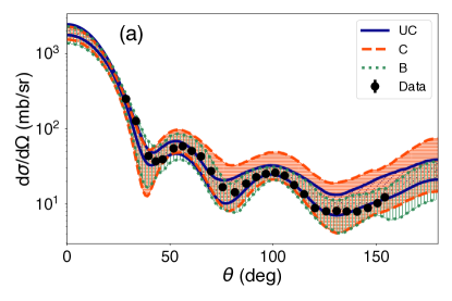
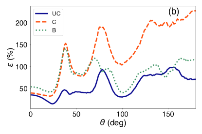
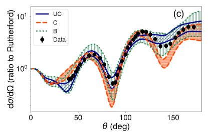
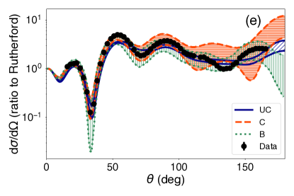
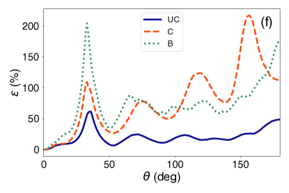
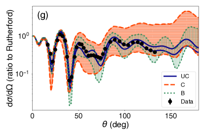
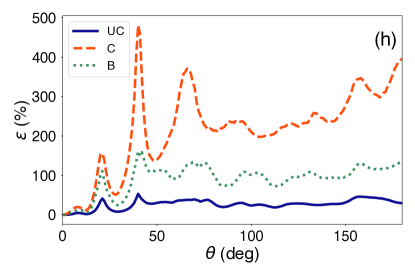
Figure 1: 95% confidence bands (left column) and percentage uncertainty (right column) for ⁴⁰Ca(n,n) at 13.9 MeV - (a) and (b) - ⁴⁰Ca(p,p) at 14.5 MeV - (c) and (d) - ⁴⁰Ca(p,p) at 26.3 MeV - (e) and (f) - and ⁴⁰Ca(d,d) at 30.0 MeV - (g) and (h). Comparison between the uncorrelated (UC, in blue), correlated (C, in red), and Bayesian (B, in green) optimizations.

In Fig. 2, we calculate the percentage of the experimental data that falls within various confidence intervals for the elastic-scattering reactions shown in Fig. 1. If the confidence intervals truthfully reproduced the uncertainties, X percent of the data would fall within the X percent confidence intervals, indicated by the solid black lines. The uncorrelated confidence intervals consistently over-predict the uncertainties for small values of the confidence intervals, below $\sim 50$%. For the neutron and proton scattering, the trends in the uncorrelated optimization are flat compared to the solid black line. The correlated optimization systematically over-predicts the uncertainty in each case except for proton scattering at 14.5 MeV, panel (b). While over-predicting the uncertainty provides a more conservative estimate, the trends in Fig. 2 are not the same across the four scattering cases.

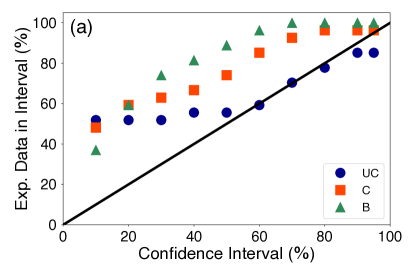
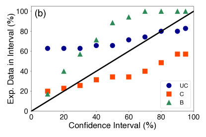
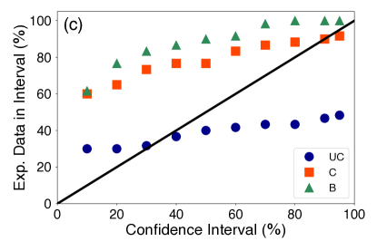
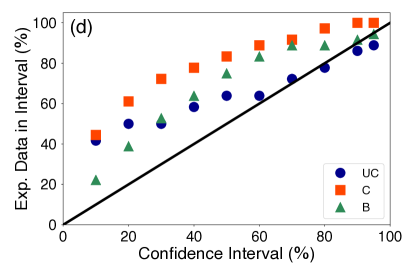
Figure 2: Percentage of the the data that falls within a given confidence interval for the uncorrelated (UC, blue circles), correlated (C, red squares), and Bayesian (B, green triangles) minimizations, for the four elastic scattering reactions studied in this work, (a) ⁴⁰Ca(n,n) at 13.9 MeV, (b) ⁴⁰Ca(p,p) at 14.5 MeV, (c) ⁴⁰Ca(p,p) at 26.3 MeV, and (d) ⁴⁰Ca(d,d) at 30.0 MeV.

These results highlight some of the shortcomings of the frequentist methods. The uncorrelated and correlated confidence intervals do not consistently predict the uncertainties. Although the uncorrelated confidence intervals give a more true representation of the uncertainties at the 1$\sigma$ level – 68% – for nucleon scattering on ⁴⁰Ca, as shown here, in [25], we found that the uncorrelated frequentist optimization consistently underpredicted the uncertainties on the elastic scattering cross sections. Thus, this test should be performed for each reaction of interest. The model covariance, as included in $\chi^{2}_{C}$, is somewhat arbitrarily defined, pointing to possible limitations of the formulation, and we ultimately do not advocate for including model correlations in this manner. In addition, these types of frequentists methods assume that the uncertainties can be described as a Gaussian distribution in parameter and observable space, which is not generally the case. Particularly, this is not true for our reaction model where the dependence of the observable (differential cross section) on the parameters (optical potential) is strongly non-linear.

For these reasons, we have also implemented a Bayesian optimization algorithm for fitting the optical potential. The Bayesian results (B) are compared to the frequentist uncorrelated and correlated results in Figs. 1 and 2: green lines or green triangles. For the Bayesian calculations, the error $\varepsilon$ is defined again as $\varepsilon=\Delta\sigma/\overline{\sigma}$, where $\Delta\sigma$ is still the width of the 95% confidence interval but now $\overline{\sigma}$ is the mean value of the cross sections within the 95% confidence interval.

In all cases, the confidence intervals and related uncertainties obtained with the Bayesian approach are larger than their frequentist counterparts (green compared to blue). Particularly at the lower uncertainty values, the uncorrelated frequentist optimization more accurately predicts the uncertainties, but if we want to look at higher confidence values – such as 2$\sigma$ or 95% confidence – the truthfulness of the uncorrelated falls off, and the Bayesian optimization becomes more reliable. In this work and our previous studies, we look at 95% confidence intervals, at which point the frequentist methods tend to underpredict the uncertainties and the Bayesian optimization is more truthful. The discrepancies between the optimization methods are also seen in the propagation of the optical model uncertainties to the single-nucleon transfer cross sections, as will be discussed in Sec. 4. These characteristics are not unique to nucleon scattering on ⁴⁰Ca, and other targets are discussed in [25].

3.2 Correlations in parameter space

It is worth also discussing the differences between the minima and correlations in parameter space among the three methods. In Table 2, we show the best-fit parameters for the uncorrelated and correlated frequentist fits along with the average parameter values from the accepted Bayesian samples. We note that, especially in the imaginary volume term, many of the parameters have to be fixed in order to prevent the minimum from going into unphysical regions of the parameter space when the frequentist optimization is used. These parameters are shown in italics in Table 2. However, the real volume term is fairly similar between the three optimization schemes, meaning that they all lead to similar minima, the biggest differences being the geometries of the potentials. Moreover, particularly in the frequentist optimization, the parameters tend to be highly correlated, leading to similar elastic-scattering cross sections, even when the geometry is not the same. We can also constrain the Bayesian optimization to have the same parameters fixed (at the same values) as the uncorrelated frequentist optimization, and when this is done, we find essentially the same minima between the two routines. We then conclude that the prior distribution – especially a very wide Gaussian prior, as we use here – does not strongly affect the minima that are found in the Bayesian optimization and does not necessarily keep the minimum closer to the starting parameter set. The Bayesian optimization procedure is data-driven (or driven by the likelihood) rather than being driven by the prior distribution, and the Bayesian procedure allows the parameters to remain in the physical region of the parameter space, while adding a very minimal constraint with the prior distribution.

In the bottom half of Table 2, we list the widths of the parameter distributions, either from the parameter covariance matrix for the frequentist calculations or the standard deviation of the set of accepted parameters for the Bayesian calculations. In most cases, the Bayesian parameters widths are larger than both the uncorrelated and correlated frequentist widths. The largest difference is for the correlated frequentist optimization, where sometimes the imaginary surface parameters are wider than the parameters found in the Bayesian optimization. Noticeably, the optimization of ⁴⁰Ca(p,p) at 14.5 MeV is the only case where all of the Bayesian parameter widths are larger than the correlated frequentist parameters, and this is the only case where the Bayesian confidence intervals are larger than the correlated confidence intervals across the full angular range.

There is a high level of degeneracy in the parameter space, both continuous and discrete, due to the fact that different sets of optical parameters can provide the same elastic scattering distribution. One way to address this degeneracy is to introduce new parameters resulting from a combination of optical potential parameters that would remove the degeneracy. This is not our approach. In fact, because we choose to use wide priors, we explore a wide region of parameter space, with all its degeneracies, and allow for multimodal posteriors. Our uncertainty intervals thus have no biases toward one or another minimum. Nevertheless, by construction the priors do not favor unphysical value for the parameters, avoiding issues with negative values for radii and diffuseness.

Optimization	Reaction	V ($\mu$)	r ($\mu$)	a ($\mu$)	Ws ($\mu$)	rs ($\mu$)	as ($\mu$)	Wv ($\mu$)	rW ($\mu$)	aW ($\mu$)
UC	40Ca(n,n) (13.9)	45.629	1.293	0.500	3.959	1.129	0.890	1.289	1.094	0.301
C	40Ca(n,n)	43.284	1.316	0.532	4.303	1.111	0.789	1.301	1.332	0.652
B	40Ca(n,n)	44.246	1.317	0.550	7.268	1.231	0.484	1.276	1.095	0.587
UC	40Ca(p,p) (14.5)	53.286	1.160	0.590	2.145	1.279	0.892	1.189	1.070	0.757
C	40Ca(p,p)	52.467	1.267	0.488	2.008	1.045	0.7849	2.088	1.118	0.652
B	40Ca(p,p)	51.472	1.207	0.639	6.471	1.312	0.371	0.425	1.335	0.530
UC	40Ca(p,p) (26.3)	55.776	1.067	0.881	4.206	1.034	0.721	4.421	1.3121	0.51
C	40Ca(p,p)	44.676	1.258	0.7077	6.7437	1.210	0.403	2.588	1.362	0.7556
B	40Ca(p,p)	56.538	1.025	0.865	3.027	1.591	0.602	3.408	1.390	0.483
UC	40Ca(d,d) (30.0)	97.936	1.065	0.805	9.045	1.516	0.630	2.444	1.479	0.311
C	40Ca(d,d)	100.49	1.077	0.774	6.624	1.413	0.853	2.010	1.600	0.334
B	40Ca(d,d)	97.026	1.080	0.782	9.697	1.486	0.676	2.617	1.045	0.555
		V ($\sigma$)	r ($\sigma$)	a ($\sigma$)	Ws ($\sigma$)	rs ($\sigma$)	as ($\sigma$)	Wv ($\sigma$)	rW ($\sigma$)	aW ($\sigma$)
UC	40Ca(n,n) (13.9)	2.426	0.045	0.048	0.722	0.185	—	—	—	—
C	40Ca(n,n)	2.022	0.029	0.076	1.210	0.203	0.237	—	—	—
B	40Ca(n,n)	3.277	0.057	0.057	0.604	0.086	0.038	0.150	0.106	0.069
UC	40Ca(p,p) (14.5)	1.475	0.016	0.024	0.309	0.170	—	—	—	—
C	40Ca(p,p)	1.889	0.020	0.017	0.202	—	—	—	—	—-
B	40Ca(p,p)	2.915	0.047	0.060	0.648	0.114	0.053	0.046	0.154	0.059
UC	40Ca(p,p) (26.3)	2.245	0.027	0.023	0.210	—	—	—	—	—
C	40Ca(p,p)	1.062	0.027	0.031	1.243	0.035	0.050	—	—	—
B	40Ca(p,p)	3.622	0.044	0.050	0.446	0.096	0.058	0.285	0.098	0.058
UC	40Ca(d,d) (30.0)	5.361	0.043	0.023	0.511	0.015	0.026	—	—	—-
C	40Ca(d,d)	5.743	0.127	0.095	—	0.155	0.148	—	—	—
B	40Ca(d,d)	7.269	0.056	0.038	0.950	0.042	0.054	0.299	0.144	0.051

Table 2: Optimized parameter means, $\mu$, and and posterior widths, $\sigma$, for each of the three fitting techniques (first column) and each reaction studied (incident energies, in MeV, listed in parentheses in the second column). The real volume, imaginary surface, and imaginary volume depths are listed, in MeV, in the third, sixth, and ninth columns, respectively. The corresponding radii (diffusenesses) are listed in fm in the fourth (fifth), seventh (eighth), and tenth (eleventh) columns.

In addition, the correlations between the parameters from the four elastic-scattering optimizations are shown in Fig. 3. To focus on the differences in the correlations and not the parameter values, the correlations have been normalized such that each mean is zero and the width of the distribution is one. Circular distributions indicate uncorrelated parameters while the more oval distribution indicate more correlated (or anti-correlated) parameter pairs. Historically, the optical model parameters had been found to be extremely correlated [43], and these correlations can be seen in the blue and red distributions of the uncorrelated and correlated parameters. On the other hand, the Bayesian optimization shows very few correlations, except between the depth and radius of the real volume potential. This lack of correlation was also seen in [25] and indicates that strong correlations may have been induced by the $\chi^{2}$ minimization procedure.

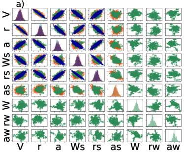
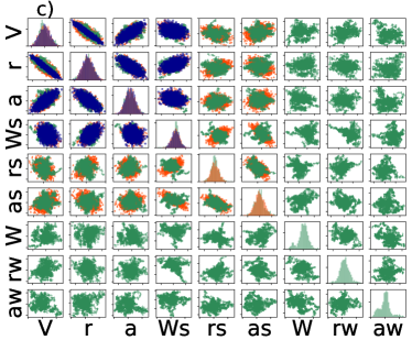
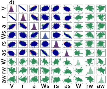
Figure 3: Correlations between the optical model parameters for (a) ⁴⁰Ca(n,n) at 13.9 MeV, (b) ⁴⁰Ca(p,p) at 14.5 MeV, (c) ⁴⁰Ca(p,p) at 26.3 MeV, and (d) ⁴⁰Ca(d,d) at 30.0 MeV for the uncorrelated, correlated, and Bayesian optimizations in blue, red, and green respectively. Histograms on the diagonal and parameters in the off-diagonal scatter plots have been normalized to mean zero and standard deviation one to emphasize the differences in the correlations.

Now that we have seen the uncertainties coming from the optical potential with the constraints coming from fitting the differential cross sections, we find that these uncertainties are so large as to be almost unusable. The uncertainties that we have found in all studied cases have varied anywhere from 20% to over 100% - and are not any smaller when they are propagated to the single-nucleon transfer cross sections. Therefore, we have also been exploring ways to reduce the uncertainties in the optical potential. In the next two subsections, we discuss further experimental constraints to shrink the uncertainties on the optical potential - and the resulting uncertainties on the elastic scattering and transfer cross sections.

3.3 Other experimental constraints on the optical potential

Next we explore experimental conditions for elastic-scattering measurements, with the intent of reducing the uncertainties. Here we include tests on the angular range of the data fitted and the effects of including a second set of elastic angular distributions, obtained at a nearby energy.

The angular range of the data included in the optimization procedure in [49], tested whether fitting only angles forward of 100^∘ or fitting a reduced set of angular data (where every other angular data point was removed) produced significant differences in the width of the uncertainty interval. Because of the correlations between the differential cross section at various angles, due to the partial wave decomposition, constrains at one angle are propagated to other angles. Consistent with that, we find that we do not gain more information with a denser angular grid, and constraining backwards angles expectedly only affects the backward angle uncertainty.

Instead, we turn to including a second set of elastic-scattering data at a nearby energy. There are two ways to include this second set: 1) sequentially, where the Bayesian optimization is run using the first set of data and the parameter posterior distribution is used as the prior distribution to optimize over the second set of data, or 2) simultaneously, where the two data sets are both fed into the optimization routine at the same time. When the two data sets are included sequentially, we find a very small improvement in the uncertainties (decrease in the size of the confidence intervals), just as in [49]. However, while [49] shows a large improvement when the two data sets are included simultaneously, in the cases studied here we find only a modest improvement. This is illustrated in Fig. 4: a simultaneous fit (denoted multiple, red) is compared to the fitting of only one data set (single, blue) in for ⁴⁰Ca(n,n) at 13.9 MeV (a) and ⁴⁰Ca(p,p) at 14.5 MeV (c). In panels (b) and (d), we show the percent uncertainty of the confidence intervals, $\varepsilon$.

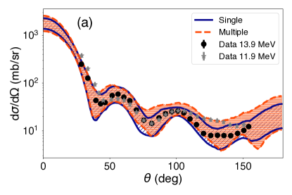
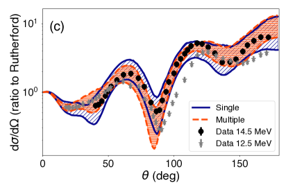
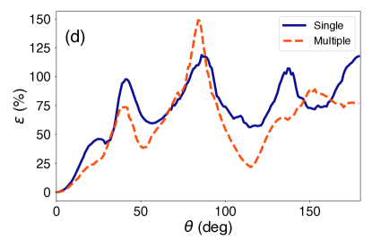
Figure 4: Comparison between the Bayesian optimization of a single elastic scattering data set (single, blue) and the simultaneous optimization of two nearby energies (multiple, red) for (a) ⁴⁰Ca(n,n) at 13.9 MeV (second set at 11.9 MeV), and (c) ⁴⁰Ca(p,p) at 14.5 MeV (second set at 12.5 MeV). In (b) and (d) are the corresponding percentage uncertainties, $\varepsilon$.

As is evident from the percent uncertainty in panels (b) and (d) for the neutron scattering and proton scattering respectively, no significant decrease in the uncertainty is found when the second set of experimental data is included. In particular, for the neutron scattering case, we actually see an increase of the uncertainties at backwards angles. This increase is due to the discrepancies between the two data sets backwards of $100^{\circ}$ (shown as the black and grey symbols). In both cases, we used data that was measured by the same group with the same experimental set-up, to remove as many sources of systematic uncertainty as possible. The differences between the results here and the results in our previous work [49] are mainly due to the use of mock data in the previous work and real experimental data here. We discuss this further in Section 3.5.

3.4 Including a variety of reaction observables

Within the Bayesian framework, we can study how various additional experimental constraints can impact - and hopefully reduce - the uncertainties in the optical potential. The first experimental constraint that we explore is adding other reaction data to the fitting procedure. We will start first considering vector analyzing powers, $Re(iT_{11})$, and then add total or reaction cross sections, $\sigma_{\mathrm{tot}}$ or $\sigma_{\mathrm{R}}$. The combined $\chi^{2}$ applies equal weights to the different sets of data. Although the vector analyzing powers should be more sensitive to the spin-orbit part of the potential than the differential cross sections or the total and reaction cross sections, for consistency within this work, we still only optimize the volume and surface terms of the optical potential.

In Fig. 5, we show the differential cross sections (left column) and analyzing powers (right column) when only the differential cross section is fit (blue), only the polarization is fit (red), and both are fit simultaneously (green) for ⁴⁰Ca(n,n) at 13.9 MeV and ⁴⁰Ca(p,p) at 14.5 MeV. First, we notice that in (a) and (c) the best representation of the data is when only the differential cross section is fit; likewise, in panels (b) and (d), the best representation of the polarization data is when only the polarization data is included in the optimization. These are the sorts of difficulties that can arise when addressing the real problem, with real data. In both the neutron and proton scattering cases, we see that the minima are shifted significantly from the differential cross section to the polarization minimum. When both observables are included in the Bayesian optimization (green regions), the confidence intervals and posterior distributions typically fall somewhere between the minima from the elastic cross section and polarization, as for ⁴⁰Ca(p,p) at 14.5 MeV in Fig. 5(c) and (d). However, as for ⁴⁰Ca(n,n) at 13.9 MeV, in panels (a) and (b), we find that the confidence intervals when both observables are included in the fitting process are similar in shape to the confidence intervals when only the analyzing power is included in the optimization. The authors in [29], [31], and , [33] all found that for ⁴⁰Ca-nucleon scattering reactions, an optical potential of the form that we are investigating here (e.g. local, energy-dependent, and non-relativistic) was not sufficient to describe both their differential cross section data and polarization data simultaneously. These joint optimizations should be studied for other targets.

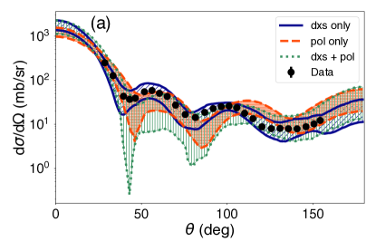
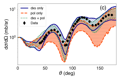
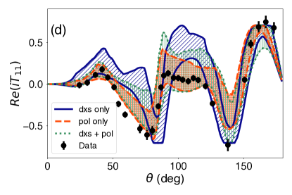
Figure 5: Comparison of the differential cross sections (a) and (c) and polarization analyzing powers (b) and (d) when only differential cross section data was fit (blue), only polarization data was fit (red), and both differential cross section and polarization data were fit, for ⁴⁰Ca(n,n) at 13.9 MeV, (a) and (b), and for ⁴⁰Ca(p,p) at 14.5 MeV, (c) and (d).

We have also considered the effect of including total or reaction cross sections along with polarization. In [49], we found that adding the reaction or total cross section into the Bayesian optimization routine did not offer an improvement on the uncertainties, when compared to the use of the full angular distribution. In that work, mock data was used and thus the total (reaction) cross section did not contain additional information to the differential cross section over all angles (by construction that total cross section was exactly the integral of the angular distribution included in the fit already). Although here we are using real data, we have chosen cases for which the angular distributions have full coverage, and therefore again, when including total (reaction) cross sections to the likelihood, the reduction on the uncertainties is minimal.

3.5 Differences between mock data and measured data

Some of the results presented in this section are significantly different than those obtained in [49], particularly when multiple energies were included in the optimization. We had previously found that fitting data at two nearby energies reduced the uncertainty on the differential cross section by as much as - and sometimes more than - 50%. Those results were calculated using mock data generated from the Koning-Delaroche optical potential [28] to ensure that we could remove any difficulties coming from discrepancies in experimental data (such as the error in the normalization, the incident energies not lining up, etc.). In Fig. 6, we show the single and multiple optimization for ⁴⁰Ca(n,n) at 13.9 MeV and ⁴⁰Ca(p,p) at 14.5 MeV using mock data: confidence intervals in panels (a) and (c) and the percentage uncertainty in (b) and (d). Comparing this figure with Fig. 4 - same calculation but with real experimental data - we see that the uncertainties are smaller when mock data are used compared to the case when real experimental data are used. In both cases though, we do not see the same degree of reduction in the uncertainty when a second energy is included in the optimization process.

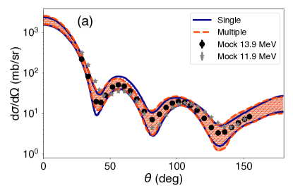
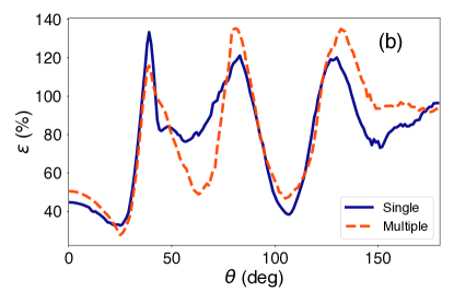
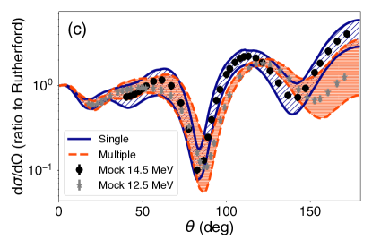
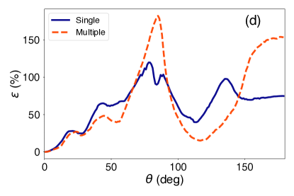
Figure 6: Comparison between the Bayesian optimization of a single elastic scattering data set (single, blue) and the simultaneous optimization of two nearby energies (multiple, red) for (a) ⁴⁰Ca(n,n) mock data at 13.9 MeV (second set at 11.9 MeV), and (c) ⁴⁰Ca(p,p) mock data at 14.5 MeV (second set at 12.5 MeV). In (c) and (d) are the corresponding percentage uncertainties, $\varepsilon$.

However, in [49], we also found that the uncertainty was strongly dependent on the percent difference between the two energies that are included in the fit. There was a greater impact at higher incident energies and when the two energies included were $\sim$ 10% apart (if the difference in energies were higher the two minima would be too different as the optical potentials are strongly energy dependent, if it were lower it would offer no extra information to the optimization procedure). With real experimental data we cannot control this. Indeed, the existing data for this case is slightly farther apart than 10%, which may also contribute to the differences seen here compared to [49]. Having a targeted experimental study to measure elastic scattering at two close energies could help us understand if these results are due to using real experimental data (not mock data) or from the percent difference between the two incident energies.

4 Solving the few-body scattering problem

Using the potential parameters that led to the cross sections shown in Fig. 1, we can propagate the uncertainties to the single-neutron transfer cross section, ⁴⁰Ca(d,p)⁴¹Ca(g.s.) at 28.4 MeV. In this section, we consider two different three-body approximations to $(d,p)$ reaction, as discussed in Section 2, namely the distorted-wave Born approximation (DWBA) and the adiabatic wave approximation (ADWA). In DWBA, the incoming channel requires the deuteron-target distorted wave while ADWA requires as input the proton-target and neutron-target distorted waves. We compare DWBA and ADWA using both the uncorrelated frequentist and Bayesian optimizations, Fig. 7 (a) and (b) respectively. Typically, a spectroscopic factor would be extracted by normalizing the calculation to the data at forward angles. However, because there is no data near this incident energy to compare to, we consider the spectroscopic factors in each case to be unity and focus on the differences in the shape of the resulting cross sections.

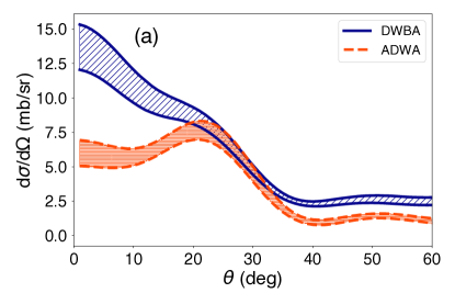
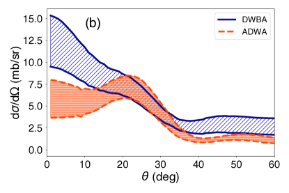
Figure 7: Comparison between the ⁴⁰Ca(d,p)⁴¹Ca(g.s.) at 28.4 MeV cross section using DWBA (blue) and ADWA (red) for (a) the uncorrelated frequentist optimization and (b) the Bayesian optimization.

When the optical potential uncertainties are propagated through each reaction formulation, we see a significant difference in shape of the angular distributions between the DWBA and ADWA calculations, for both the frequentist and Bayesian techniques. However, depending on the angular range over which the experimental data would be measured, these calculations would still be difficult to distinguish, unless a detailed angular distribution could be measured between zero and 40 degrees. For stable targets, this is certainly feasible, but when considering reactions with unstable beams where the experimental errors are typically larger and the angular coverage is reduced due to the reaction being measured in inverse kinematics, these two models will become increasingly difficult to distinguish. (Comparisons between the uncorrelated and correlated frequentist optical potentials show similar angular dependence for the DWBA and ADWA calculations, but the confidence intervals are significantly wider when the correlated fit is propagated, as would be expected from the confidence intervals on the elastic scattering in Fig. 1). It is clear that the larger uncertainties on the elastic scattering calculations translate to larger uncertainties on the transfer cross section, even though these uncertainties are propagated in a non-linear fashion.

5 The overlap function and interplay of other degrees of freedom

The last two items to consider are the overlap functions and the interplay of degrees of freedom that are left out of the model space. For single-nucleon transfer reactions, when we discuss the overlap function, we are thinking in particular of the bound-state wave function between the target and the transferred nucleon. Typically, this interaction is assumed to have a Woods-Saxon shape with a standard geometry and a depth that reproduces the nucleon-target binding energy. In [22], we showed that changing the geometry while keeping the binding energy fixed could drastically change the resulting transfer cross section, by a factor of two or more at the peak of the angular distribution. These differences were seen when the radius parameter was changed from 1.1 fm to 1.3 fm. Between the two cases that were studied, the changes were larger in the more exotic target, ¹³²Sn, compared to the stable target, ⁴⁸Ca.

We would like to study the uncertainties in the description of the bound state in a Bayesian manner. One option to incorporate these uncertainties would be to sample the geometry of the single-particle potential, constrained by narrow prior distributions for the radius and diffuseness, and imposing that the potential depth reproduces the binding energy. But one could also use constraint of other known properties. The asymptotic normalization coefficient (ANC) provides one such constraint. Previous reaction studies have shown that breakup cross sections are scaled by the ANC squared [54, 55]. Since the ANC can be calculated microscopically for light nuclei [56] and can be extracted unambiguously from peripheral reactions for many other nuclei [57], the ANC constrain could strongly reduce the ambiguity in the singe-particle potential. The effects of using the ANC as a constraint can be quantified with the current tools (similarly to what was done in [49]). Were this to provide a significant constraint on the single-particle potential, it would give a strong motivation to develop a program to measure this quantity for a variety of heavy nuclei. In addition, the overlap function can be extracted from the one-body density matrix (OBDM) [58, 59, 60], which has already been calculated for the ⁴⁰Ca target studied in this work. Extracting the uncertainties on the overlap function using both of these methods could provide an interesting comparison between the two constraints.

The last source of uncertainty in few-body reactions discussed in Section 1 comes from the degrees of freedom left out of the model space. The most obvious source of this uncertainty is the reduction of the many-body model space to a few-body problem. If one could compare exact many-body calculations directly with the few-body calculations, it would allow us to construct an emulator to connect the few-body to the many-body calculations (which typically contains an uncertainty estimate such as from a Gaussian Process [61]). Unfortunately, this is currently not possible for any but the lightest systems and given the computational scale of ab-initio reaction calculations it would take an unfeasibly long time.

Instead, what can be done effectively is to test different levels of approximations in the few-body models. We have begun to explore the differences between DWBA and ADWA calculations, two of the few-body approximations that are commonly made. The study discussed in Sec. 4 explores the differences in the uncertainty interval of the predicted cross sections when one used deuteron optical potential uncertainties versus nucleon optical potential uncertainties. A quantitative comparison of ADWA and DWBA can be performed more systematically using Bayesian evidence, as will be discussed briefly in the conclusions.

In the framework of model comparison, ADWA and DWBA are not relatable in the sense that they are not nested: one is not a simplification of the other. It is best to first consider nested models. In that context, the coupled-channel Born approximation (CCBA) is a useful model, because one can easily switch of the coupling to the inelastic state and reduce the model to DWBA. With the Bayesian machinery that we have put in place, we can systematically study the effects that the addition of inelastic scattering channels has on the widths and means of the confidence intervals for the cross sections. This starting point would enable the development of the methodology needed for more complex comparisons where one model is not just a subset of another.

6 Outlook

In this overview, we have described, using the example of ⁴⁰Ca elastic scattering and transfer reactions, recent progress made on quantifying uncertainties in few-body reaction theory. We have shown the development from frequentist $\chi^{2}$ minimization methods and covariance matrix propagation to a full Bayesian analysis in determining and propagating uncertainties in effective interactions. In addition, under these two frameworks, we can now directly compare how uncertainties are propagated from these interactions when various approximations to the few-body model are made, namely between the distorted-wave Born approximation and the adiabatic wave approximation. Although much work has been done, there are many exciting opportunities ahead. The long-term vision for the future of this work involves using Bayesian methodology along two major interacting thrusts: the first concerns experimental design and second is focused on improving theory itself (one might call it theory design). In this section we discuss the overarching vision and specific developments that are needed for implementing that vision.

One tool that we have identified as necessary to implement this long-term vision is calculating the Bayesian evidence for various theories. Described briefly in Sec. 2.1, the Bayesian evidence is the denominator in Bayes’ theorem, Eq. (14), which is a weighted sum over all possible models and provides a formal way of evaluating relative probabilities of different models. Bayesian evidence is a numeric formulation of Occam’s razor - a systematic way of showing that a simpler model which reproduces the data should be favored over a more complex model. However, computing the Bayesian evidence typically requires an integral over all of a model’s parameter space, a potentially computationally demanding task, particularly as the models become more complex. In addition, the interpretation of the value of the evidence is not always straight-forward. Still, being able to calculate the Bayesian evidence is an important development for our long-term uncertainty quantification vision.

In the first thrust of experimental design, there are many controllable conditions in reaction experiments (beam energy, angular range, target, etc.), and the tools developed thus far can help in determining those conditions that produce optimum sensitivity to the quantities of interest, e.g. as in [62]. The work in [49] is the first step along this direction, but other tools should be considered when assessing what combination of observables contains most information. Tools such as Principle Component Analysis (PCA) and Bayesian evidence have been successfully applied in other areas, e.g. [8, 11, 46, 63], and should be studied in the context of nuclear reactions.

The Bayesian methodology here discussed can also be extremely useful in improving theoretical models. So far, due to computational considerations, the models used have been very simple (optical model, DWBA, and ADWA). However, we understand that there is important physics that these models do not contain. Ultimately, we want to increase the complexity of the models, matching the state of the art in theory to the degree called for by the data. In other words, the model should be as sophisticated at the data requires. In addition, as we include more and more data in our analysis, there will be an increasing demand on the physics included in the model to be able to describe all observables simultaneously with the same accuracy. In order to start down this path, we will need quantitative and reliable methods for model comparison. An essential tool for performing model comparisons in the Bayesian world is the Bayesian evidence. Also, model mixing is the natural sequence from model comparison, as a robust way to incorporate the best aspects of each theory. Both of these developments, though, pose specific challenges that still need to be addressed. What to do when the models are not nested, and moreover when the models do not contain similar parameters? What are the most efficient and accurate methods to perform numerical integrals over a large parameter space? These are questions that must be investigated to ensure a robust development in this area.

References

- [1] Melendez J A, Wesolowski S and Furnstahl R J 2017 Phys. Rev. C 96(2) 024003 URL https://link.aps.org/doi/10.1103/PhysRevC.96.024003
- [2] Furnstahl R J, Klco N, Phillips D R and Wesolowski S 2015 Phys. Rev. C 92(2) 024005 URL https://link.aps.org/doi/10.1103/PhysRevC.92.024005
- [3] Wesolowski S, Klco N, Furnstahl R J, Phillips D R and Thapaliya A 2016 Journal of Physics G: Nuclear and Particle Physics 43 074001 URL http://stacks.iop.org/0954-3899/43/i=7/a=074001
- [4] Schindler M and Phillips D 2009 Annals of Physics 324 682 – 708 ISSN 0003-4916 URL http://www.sciencedirect.com/science/article/pii/S000349160800136X
- [5] Fukui T, Ogata K and Capel P 2014 Phys. Rev. C 90(3) 034617 URL http://link.aps.org/doi/10.1103/PhysRevC.90.034617
- [6] Schunck N, McDonnell J D, Higdon D, Sarich J and Wild S M 2015 The European Physical Journal A 51 1–14 ISSN 1434-601X URL http://dx.doi.org/10.1140/epja/i2015-15169-9
- [7] Bernhard J E, Moreland J S, Bass S A, Liu J and Heinz U 2016 Phys. Rev. C 94(2) 024907 URL http://link.aps.org/doi/10.1103/PhysRevC.94.024907
- [8] Sangaline E and Pratt S 2016 Phys. Rev. C 93(2) 024908 URL https://link.aps.org/doi/10.1103/PhysRevC.93.024908
- [9] Utama R, Chen W C and Piekarewicz J 2016 Journal of Physics G: Nuclear and Particle Physics 43 114002 URL http://stacks.iop.org/0954-3899/43/i=11/a=114002
- [10] Neufcourt L, Cao Y, Nazarewicz W and Viens F 2018 Phys. Rev. C 98(3) 034318 URL https://link.aps.org/doi/10.1103/PhysRevC.98.034318
- [11] Novak J, Novak K, Pratt S, Vredevoogd J, Coleman-Smith C E and Wolpert R L 2014 Phys. Rev. C 89(3) 034917 URL https://link.aps.org/doi/10.1103/PhysRevC.89.034917
- [12] Neufcourt L, Cao Y, Nazarewicz W, Olsen E and Viens F 2019 Phys. Rev. Lett. 122(6) 062502 URL https://link.aps.org/doi/10.1103/PhysRevLett.122.062502
- [13] Utama R, Piekarewicz J and Prosper H B 2016 Phys. Rev. C 93(1) 014311 URL https://link.aps.org/doi/10.1103/PhysRevC.93.014311
- [14] Lovell A E, Mohan A T and Talou P 2020 Quantifying uncertainties on fission fragment mass yields with mixture density networks (Preprint 2005.03198)
- [15] Wang Z A, Pei J, Liu Y and Qiang Y 2019 Phys. Rev. Lett. 123(12) 122501 URL https://link.aps.org/doi/10.1103/PhysRevLett.123.122501
- [16] Lasseri R D, Regnier D, Ebran J P and Penon A 2020 Phys. Rev. Lett. 124(16) 162502 URL https://link.aps.org/doi/10.1103/PhysRevLett.124.162502
- [17] Nunes F M and Deltuva A 2011 Phys. Rev. C 84(3) 034607 URL http://link.aps.org/doi/10.1103/PhysRevC.84.034607
- [18] Upadhyay N, Deltuva A and Nunes F 2012 Phys.Rev. C85 054621 (Preprint 1112.5338)
- [19] Deltuva A, Moro A M, Cravo E, Nunes F M and Fonseca A C 2007 Phys. Rev. C 76(6) 064602 URL http://link.aps.org/doi/10.1103/PhysRevC.76.064602
- [20] Capel P, Esbensen H and Nunes F M 2012 Phys. Rev. C 85(4) 044604 URL http://link.aps.org/doi/10.1103/PhysRevC.85.044604
- [21] Titus L J, Nunes F M and Potel G 2016 Phys. Rev. C 93(1) 014604 URL https://link.aps.org/doi/10.1103/PhysRevC.93.014604
- [22] Lovell A E and Nunes F M 2015 Journal of Physics G: Nuclear and Particle Physics 42 034014 URL http://stacks.iop.org/0954-3899/42/i=3/a=034014
- [23] Lovell A E, Nunes F M, Sarich J and Wild S M 2017 Phys. Rev. C 95(2) 024611 URL https://link.aps.org/doi/10.1103/PhysRevC.95.024611
- [24] Lovell A E and Nunes F M 2018 Phys. Rev. C 97(6) 064612 URL https://link.aps.org/doi/10.1103/PhysRevC.97.064612
- [25] King G B, Lovell A E, Neufcourt L and Nunes F M 2019 Phys. Rev. Lett. 122(23) 232502 URL https://link.aps.org/doi/10.1103/PhysRevLett.122.232502
- [26] King G B, Lovell A E and Nunes F M 2018 Phys. Rev. C 98(4) 044623 URL https://link.aps.org/doi/10.1103/PhysRevC.98.044623
- [27] Becchetti FD J and Greenlees G 1969 Phys.Rev. 182 1190–1209
- [28] Koning A and Delaroche J 2003 Nucl.Phys. A713 231–310
- [29] Tornow W, Woye E, Mack G, Floyd C, Murphy K, Guss P, Wender S, Byrd R, Walter R, Clegg T and Leeb H 1982 Nuclear Physics A 385 373 – 406 ISSN 0375-9474 URL http://www.sciencedirect.com/science/article/pii/0375947482900938
- [30] McDonald W and Robson J 1964 Nuclear Physics 59 321 – 331 ISSN 0029-5582 URL http://www.sciencedirect.com/science/article/pii/0029558264900872
- [31] Aoki Y, Hirota K, Kishita H, Koyama K, Masaki M, Miura K, Mukouhara Y, Nakagawa S, Okumura N and Tagishi Y 1996 Nuclear Physics A 599 417 – 434 ISSN 0375-9474 URL http://www.sciencedirect.com/science/article/pii/0375947495004793
- [32] Dicello J F and Igo G 1970 Phys. Rev. C 2(2) 488–499 URL https://link.aps.org/doi/10.1103/PhysRevC.2.488
- [33] McCamis R H, Nasr T N, Birchall J, Davison N E, van Oers W T H, Verheijen P J T, Carlson R F, Cox A J, Clark B C, Cooper E D, Hama S and Mercer R L 1986 Phys. Rev. C 33(5) 1624–1633 URL https://link.aps.org/doi/10.1103/PhysRevC.33.1624
- [34] Carlson R F, Cox A J, Nimmo J R, Davison N E, Elbakr S A, Horton J L, Houdayer A, Sourkes A M, van Oers W T H and Margaziotis D J 1975 Phys. Rev. C 12(4) 1167–1175 URL https://link.aps.org/doi/10.1103/PhysRevC.12.1167
- [35] Röche R, Sen] N V, Perrin G, Gondrand J, Fiore A and Müller H 1974 Nuclear Physics A 220 381 – 390 ISSN 0375-9474 URL http://www.sciencedirect.com/science/article/pii/037594747490726X
- [36] Summers N C, Nunes F M and Thompson I J 2006 Phys. Rev. C 74(1) 014606 URL http://link.aps.org/doi/10.1103/PhysRevC.74.014606
- [37] Summers N C, Nunes F M and Thompson I J 2014 Phys. Rev. C 89(6) 069901 URL http://link.aps.org/doi/10.1103/PhysRevC.89.069901
- [38] Moro A M and Lay J A 2012 Phys. Rev. Lett. 109(23) 232502 URL http://link.aps.org/doi/10.1103/PhysRevLett.109.232502
- [39] Deltuva A 2009 Phys. Rev. C 79(5) 054603 URL https://link.aps.org/doi/10.1103/PhysRevC.79.054603
- [40] Titus L J and Nunes F M 2014 Phys. Rev. C 89(3) 034609 URL http://link.aps.org/doi/10.1103/PhysRevC.89.034609
- [41] Mahzoon M H, RJCharity, WHDickhoff, HDussan and SJWaldecker 2014 Phys. Rev. Lett. 112 162503
- [42] Rotureau J, Danielewicz P, Hagen G, Jansen G R and Nunes F M 2018 Phys. Rev. C 98(4) 044625 URL https://link.aps.org/doi/10.1103/PhysRevC.98.044625
- [43] Thompson I J and Nunes F M 2009 Nuclear Reactions for Astrophysics: Principles, Calculation and Applications of Low-Energy Reactions Cambridge University Press
- [44] Johnson R and Tandy P 1974 Nuclear Physics A 235 56 – 74 ISSN 0375-9474 URL http://www.sciencedirect.com/science/article/pii/037594747490178X
- [45] Sivia D S 1996 Data Analysis: A Bayesian Tutorial (Oxford Science Publications)
- [46] Trotta R 2008 Contemporary Physics 49 71–104 (Preprint http://dx.doi.org/10.1080/00107510802066753) URL http://dx.doi.org/10.1080/00107510802066753
- [47] Metropolis N, Rosenbluth A W, Rosenbluth M N, Teller A H and Teller E 1953 The Journal of Chemical Physics 21 1087–1092 (Preprint http://dx.doi.org/10.1063/1.1699114) URL http://dx.doi.org/10.1063/1.1699114
- [48] HASTINGS W K 1970 Biometrika 57 97–109 URL + http://dx.doi.org/
- [49] Catacora-Rios M, King G B, Lovell A E and Nunes F M 2019 Phys. Rev. C 100(6) 064615 URL https://link.aps.org/doi/10.1103/PhysRevC.100.064615
- [50] An H and Cai C 2006 Phys. Rev. C 73(5) 054605 URL https://link.aps.org/doi/10.1103/PhysRevC.73.054605
- [51] James F 1994 CERN Program Library Long Writeup D 506
- [52] Thompson I 2006 www.fresco.org.uk
- [53] Titus L, Ross A and Nunes F 2016 Comput. Phys. Commun. 207 499 – 517 ISSN 0010-4655 URL http://www.sciencedirect.com/science/article/pii/S0010465516302028
- [54] Capel P and Nunes F M 2006 Phys. Rev. C 73(1) 014615 URL https://link.aps.org/doi/10.1103/PhysRevC.73.014615
- [55] Capel P and Nunes F M 2007 Phys. Rev. C 75(5) 054609 URL https://link.aps.org/doi/10.1103/PhysRevC.75.054609
- [56] Brida I, Pieper S C and Wiringa R B 2011 Phys. Rev. C 84(2) 024319 URL https://link.aps.org/doi/10.1103/PhysRevC.84.024319
- [57] Mukhamedzhanov A M and Nunes F M 2005 Phys. Rev. C 72(1) 017602 URL http://link.aps.org/doi/10.1103/PhysRevC.72.017602
- [58] Ivanov M V, Gaidarov M K, Antonov A N and Giusti C 2001 Phys. Rev. C 64(1) 014605 URL https://link.aps.org/doi/10.1103/PhysRevC.64.014605
- [59] Timofeyuk N and Johnson R 2020 Progress in Particle and Nuclear Physics 111 103738 ISSN 0146-6410 URL http://www.sciencedirect.com/science/article/pii/S0146641019300730
- [60] Dimitrova S S, Gaidarov M K, Antonov A N, Stoitsov M V, Hodgson P E, Lukyanov V K, Zemlyanaya E V and Krumova G Z 1997 Journal of Physics G: Nuclear and Particle Physics 23 1685–1695 URL https://doi.org/10.1088%2F0954-3899%2F23%2F11%2F016
- [61] Rasmussen C E and Williams K I 2006 Gaussian Processes for Machine Learning (The MIT Press)
- [62] Melendez J A, Furnstahl R J, Grießhammer H W, McGovern J A, Phillips D R and Pratola M T 2020 Designing optimal experiments: An application to proton compton scattering (Preprint 2004.11307)
- [63] Fox J M R, Johnson C W and Perez R N 2020 Phys. Rev. C 101(5) 054308 URL https://link.aps.org/doi/10.1103/PhysRevC.101.054308