Particle spectra from dark matter annihilation: physics modeling and QCD uncertainties

Abstract

In this talk, we discuss the physics modelling of particle spectra arising from dark matter (DM) annihilation or decay. In the context of the indirect searches of DM, the final state products will, in general, undergo a set of complicated processes such as resonance decays, QED/QCD radiation, hadronisation and hadron decays. This set of processes lead to stable particles (photons, positrons, anti-protons, and neutrinos among others) which travel for very long distances before reaching the detectors. The modelling of their spectra contains some uncertainties which are often neglected in the relevant analyses. We discuss the sources of these uncertainties and estimate their impact on photon energy spectra for benchmark DM scenarios with $m_{\chi}\in[10,1000]\,$GeV. Instructions for how to retrieve complete tables from Zenodo are also provided.

1 Introduction

Various gravitational, astrophysical and cosmological observations strongly imply the existence of Dark Matter (DM) in the universe. In particular, observations of the cosmological scale structure favour the so-called cold DM (CDM) scenario where the DM was not relativistic in the era of structure formation. In particle physics framework, the CDM scenario can be easily accounted for by extending the Standard Model (SM) with weakly interacting massive particles (WIMPs) – for a review see e.g. [1] –. An interesting feature of the CDM scenario is that WIMPs with mass about $\mathcal{O}(100)~{}$GeV interacting primarily through weak interactions gives relic abundance of DM in agreement with the observation made by the Planck satellite, i.e. $\Omega_{\mathrm{DM}}h^{2}=0.1188\pm 0.0010$ [2].

Indirect detection experiments such as the Fermi Large Area Telescope (LAT) [3], AMS [4] or IceCube [5] provide one the possible ways to detect WIMPs. Theoretically, WIMPs undergo either annihilation [6, 7], co-annihilations [8], or decays [9, 10] into a set of SM stable final state particles such as high energy photons, positrons, neutrinos, or anti-protons. Recently, an excess on the gamma-ray spectra was detected by the Fermi-LAT [11], called the Galactic Center Excess (GCE) which apparently seem to be consistent with predictions from DM annihilation (see e.g. [12]). On the other hand, several attempts were made to address the GCE within particle physics models, in particular within supersymmmetric models [16, 15, 14, 13]. An important finding is that the quality of the fits depend crucially on the theoretical precision on the determination of the gamma-ray spectra [16].

Particle production from DM annihilation/decay processes is dominated by QCD jet fragmentation. Final state stable particles such as photons or positrons are then produced as a result of a complicated set of processes which includes QED and QCD radiations, hadronisation, and hadron decays. Unlike parton-level scattering amplitudes at e.g. the lowest order of perturbation theory, the problem of hadronisation cannot be solved from first-principles. Jet universality tells us that hadronisation is a universal process that can be factorised off the short-distance processes e.g. DM annihilation. Phenomenological models such that Fragmentation Functions [17] or explicit dynamical models such as the string [19, 18] or cluster [21, 20] models which are embedded in Monte Carlo (MC) event generators [22] are the up-to-date solutions to the hadronisation problem. The essential point is that the fragmentation models’ parameters are to a very good approximation independent of the short-distance processes; therefore, they can be determined from fits to existing data such as $e^{+}e^{-}\to\mathrm{hadrons}$ and used to make predictions for e.g. DM annihilation.

The question of the intrinsic QCD uncertainties on the predicted particle spectra in DM annihilation is often neglected in the literature besides some comparisons between the predictions of different multi-purposes event generators such as Herwig and Pythia. For instance, a comprehensive analysis has shown that different MC event generators may have excellent agreement in both the peak as well as the bulk of the spectra while their agreement is not very good in the tails [23]. Another study was done by the authors of the PPPC4DMID [24] where they highlighted the differences between Herwig and Pythia event generators. The excellent level of agreement in the most-populated regions of particle spectra may be interpreted as due to the fact that the different MC generators tend to be tuned to roughly the same set of data mostly coming from LEP measurements at the $Z$-boson pole [25, 26, 27, 28, 29, 31, 30, 32, 34, 33]. Therefore, the envelope spanned by the predictions of the different MC models cannot represent the true estimate of the uncertainty on the predicted spectra.

In this talk, we discuss a first study of the QCD uncertainties on particle spectra from DM annihilation within the same MC model. We take the default Monash 2013 tune [31] of the Pythia version 8.2.35 event generator [36] as our baseline. We use a selection of experimental measurements constraining from $e^{+}e^{-}$ colliders preserved in the Rivet [26] analysis package combined with the Professor [25] parameter optimisation tool. Then, we define a small set of the systematic parameter variations which we argue that explores the uncertainty envelope for the estimate of the QCD fragmentation uncertainties on DM annihilation.

QED bremsstrahlung	QCD fragmentation and hadron decays
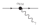
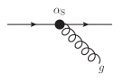
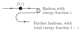
Dominates at high $x_{\gamma}$	Photons from $\pi^{0}\to\gamma\gamma$ dominate bulk (and peak) of spectra

Figure 1: Illustration of the main parameters that affect the photon spectra ($x_{\gamma}=E_{\gamma}/m_{\chi}$) from DM annihilation into jets. Here we show the electromagnetic coupling $\alpha_{\mathrm{EM}}$ (left), the strong coupling $\alpha_{S}$ (middle), and the nonperturbative fragmentation function $f(z)$ (right).

2 Physics Modeling and Measurements

2.1 Physics modeling

In this section, we discuss briefly the physics modeling in a generic DM annihilation, and the origin of photons (a more detailed discussion can be found in [35]). To simplify the discussion, we consider a generic DM annihilation process:

$$\chi\chi\to X_{1}\cdots X_{n}\to\displaystyle\prod_{i=1}^{m}Y_{1i}\cdots Y_{ni}$$

where we factorised the whole process into a production part $\chi\chi\to X_{1}\cdots X_{n}$, and the decay part ($X_{i}\to Y_{i1}\cdots Y_{in}$ with $Y_{ij}$ is any stable object such as photon, neutrino or proton) assuming the narrow-width approximation. We note three important processes which may occur after DM annihilation and responsible for gamma-rays:

• QED bremsstrahlung: This process occurs if $X$ (or the decay products $Y$) contains photons or electrically charged particles. Additional photons are produced via $X_{i}^{\pm}\to X_{i}^{\pm}\gamma$ branchings with probabilities that are enhanced for both soft and collinear photons. On the other hand, collinear photons dominate the spectra at the region $x_{\gamma}\to E_{\gamma}/m_{\chi}\to 1$ with the only requirement that the angle between the emitted photon and the parent particle is very small. QED processes may lead to the production of charged fermion-antifermion pairs in photon splittings (which are generally subleading) and the corresponding probabilities are enhanced at very low values of $Q^{2}=(p_{f}+p_{\bar{f}})^{2}$. The rates of QED processes are governed by the effective electromagnetic fine-structure constant, $\alpha_{\mathrm{EM}}$ (illustrated in Fig. 1a).

• QCD showers: If $X$ (or decay products $Y$) contains coloured particles, then these states will undergo QCD showers. The modeling of the QCD showers is similar to the QED one. Here, we can have enhancement of soft and collinear emissions – in $q\to qg$ and $g\to gg$ – and of $g\to q\bar{q}$ at low virtualities. The main parameter governing the QCD showering is the effective value of the strong coupling constant, $\alpha_{S}$ (see Fig. 1b) evaluated at a scale proprtional to the shower evolution variable ($p_{\perp}$ in Pythia8). Further sets of universal corrections in the soft limit implies that the strong coupling should be defined in the CMW [37] rather than the conventional $\overline{\mathrm{MS}}$ scheme. Furthermore, good agreement between Pythia8 and experimental measurements of $e^{+}e^{-}\to 3~{}\mathrm{jets}$ [27, 31] increases the value of $\alpha_{S}(M_{Z})$ by about $10\%$. Perturbative uncertainty estimates can be performed by variation of the evolution of the renormalisation by a factor of $2$ in each direction with respect to the nominal scale choice. The framework of the automated scale variations was recently implemented in Pythia [38] implies a compensation of second-order terms which reestablishes the agreement with the CMW scheme. Variations of the no-universal (no-singular) components of the Dokshitzer-Gribov-Lipatov-Altarelli-Parisi (DGLAP) splitting kernels can be performed in this framework as it is detailed in [38].

• Hadronisation and hadron decays: Any produced coloured particles must be confined inside colourless hadrons. This process — hadronisation — takes place at a distance scale of order the proton size $\sim 10^{-15}$m and in Pythia is modelled by the Lund string model; see [18] for details. The most majority of photons are produced from the decays of neutral pions where the number and energy of these photons are strongly correlated with the predicted pion spectra. The description of this process is embedded in the fragmentation function, $f(z)$, which gives the probability for a hadron to take a fraction $z\in[0,1]$ of the remaining energy at each step of the (iterative) string fragmentation process (see Fig. 1c). The fragmentation function $f(z)$ cannot calculated from first principles but its form can be constrained by requirements such as causality. The general form can be written as

  $$f(z,m_{\perp h})=N\frac{(1-z)^{a}}{z}\exp\left(\frac{-bm_{\perp h}^{2}}{z}\right)~{},$$ (1)

  where $N$ is a normalisation constant that guarantees the distribution to be normalised to unit integral, and $m_{\perp h}=\sqrt{m_{h}^{2}+p_{\perp h}^{2}}$ is called the “transverse mass”, with $m_{h}$ the mass of the produced hadron and $p_{\perp h}$ its momentum transverse to the string direction, $a$ and $b$ are tunable parameters which will be denoted respectively by StringZ:aLund and StringZ:bLund. We note that the $a$ and $b$ parameters are extremely highly correlated. This makes it meaningless to assign independent $\pm$ uncertainties on them. To address this question, we implement an alternative parametrisation of $f(z)$ where $b$ is replaced by a $<z>$ which represents the average $z$ fraction taken by $\rho$ mesons.

  $$\left<z_{\rho}\right>=\int_{0}^{1}\mathrm{d}z\ zf(z,\left<m_{\perp\rho}\right>)~{},$$ (2)

  which we solve (numerically) for $b$ at initialisation when the option StringZ:deriveBLund = on is selected in Pythia 8.235, using the following parameters:

  $$\left<m_{\perp\rho}\right>^{2} = m^{2}_{\rho}+2(\mbox{{StringPT:sigma}})^{2}~{},$$ (3)

  $$\left<z_{\rho}\right> = \mbox{{StringZ:avgZLund}}~{}.$$ (4)

2.2 Photon origins and available measurements

Here, we discuss briefly the origin of photons from DM annihilation (a very detailed discussion can be found in [35]). Most of the photons are coming from pion decays; about $88$-$95\%$ depending on the annihilation channel and on the DM mass. The contribution from $\eta$ decays is somewhat subleading which is about $4\%$. Finally, very sub-leading contributions are coming from bremsstrahlung photons and dominates in the high tail of the spectrum. Since the majority of photons ($\simeq 95\%$) are coming from pion decays, the QCD uncertainties on photon spectra is strongly correlated to those on the pion spectra. We can distinguish between primary pions directly produced from QCD fragmentation and secondary pions coming from the decays of heavier hadrons and $\tau$ leptons. In all the final states [35], the number of secondary pions is larger than primary ones. The secondary pions account for about $70\%$-$85\%$ of the total pions. We note that the secondary pions mainly come from five sources: $\rho^{\pm},\eta,\omega,D^{0,\pm}$ and $K_{S,L}$.

After discussing the origin of photons in DM annihilation, we conclude that in addition to the direct measurements of the photon spectrum, other measurements can be used to constrain the spectrum: (i) the spectrum of neutral pions ($\pi^{0}$) since they are the most dominant source of photons in QCD jets, (ii) the spectra of charged pions due to the fact that their number is related to $\pi^{0}$ by isospin symmetry and (iii) $\eta$ spectrm as they are the second-most important source of photons in QCD jets. Finally, it is important to ensure that these tunings do not produce large corrections to infrared and collinear safe observables such as e.g. the $C$-parameter. The tunings will include the full range of these observables including the back-to-back regions which are extremely sensitive to non-perturbative QCD effects. These measurements provides important constraints on the StringPT:sigma parameter in particular.

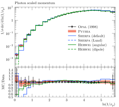
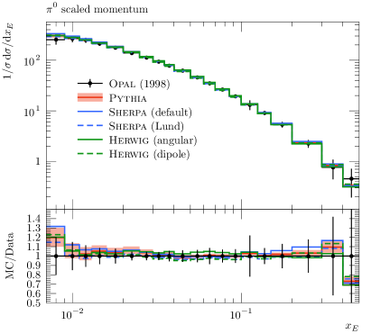
Figure 2: Comparison between MC event generators and LEP and SLD measurements for the photon spectrum (left pane), and the $\pi^{0}$ spectrum (right pane).

In Fig. 2, we compare several different multi-purpose MC event generators to measurements of two the photon and $\pi^{0}$ scaled momenta. We consider three event generators in these comparisons; Herwig 7.1.3 [39] using both the angular-ordered [44] and dipole [40, 28] shower algorithms and a cluster based hadronisation model [21], Pythia 8.2.35 with the default model of hadronisation [36] and Sherpa 2.2.5 [41] with the CSS parton shower [42] using both the Ahadic [20] (based on the cluster model) and the Pythia 6.4 Lund hadronisation [43] models. The curve corresponding to Pythia is shown with an uncertainty band (red) obtained using the results of our new tune, based on the recent Monash tune but refitting the three main hadronisation parameters (see below). We can see from Fig. 2 that the multi-purpose event generators agree pretty well except in a few regions such as e.g. in the tails towards hard high-energy photons.

3 Tuning

3.1 Setup

We used Pythia8 version 8.235 throughout this study with the most recent Monash [31] tune is used as baseline for the parameter optimisation. We use Professor v2.2 [25] to perform the tuning and Rivet v2.5.4 [26] for the implementation of the measurements. In Professor, a method permits to make simultaneous optimisation of several parameters by using analytical approximations of the dependence of the MC response on the model parameters (this idea was introduced first in Ref. [45]). In order to minimises the differences between the interpolated functions and the true MC response, we use a fourth-order polynomial. The values of the model parameters at the minimum are then obtained with a standard $\chi^{2}$ minimisation of the analytic approximation to the corresponding data using Minuit [46]. In this work, we tuned the $a$ and $b$ parameters of the Lund fragmentation function ($a$ and $<z_{\rho}>$ in the new parametrization) and the $\sigma$ parameter which governs the transverse components (see e.g. [47]). The default values of the parameters and their allowed range in Pythia8 are shown in Table 1.

To protect against over-fitting effects and as a baseline sanity limit for the achievable accuracy, we introduce an additional $5\%$ uncertainty on each bin and for each observable. This also substantially reduces the value of the goodness-of-fit measure so that the resulting $\chi^{2}/\textrm{ndf}$ is consistent with unity (see Table 2). The $\chi^{2}/N_{\textrm{DoF}}$ is defined by:

$$\frac{\chi^{2}}{N_{\textrm{DoF}}}=\frac{1}{\sum_{\mathcal{O}}\omega_{\mathcal{O}}|b\in\mathcal{O}|}\frac{\sum_{\mathcal{O}}\omega_{\mathcal{O}}\sum_{b\in\mathcal{O}}(f_{(b)}(\textbf{p})-\mathcal{R}_{b})^{2}}{(\Delta_{b}^{2}+(0.05f_{(b)}(\textbf{p}))^{2})}~{}.$$ (5)

Here $\omega_{\mathcal{O}}$ represents the weight per observable and per bin, $f_{(b)}(\textbf{p})$ is the interpolated function per bin $b$, $\mathcal{R}_{b}$ is the experimental value of the observable $\mathcal{O}$ and $\Delta_{b}$ is the experimental error per bin, with $f_{(b)}$ is the $4$th order interpolated polynomial used to model the MC response. We use various experimental measurements from Lep and Slc at the $Z$-boson peak produced by Aleph, Delphi, L3, Opal and Sld.

parameter	Pythia8 setting	Variation range	Monash
$\sigma_{\perp}$ [GeV]	StringPT:Sigma	0.0 – 1.0	0.335
$a$	StringZ:aLund	0.0 – 2.0	0.68
$b$	StringZ:bLund	0.2 – 2.0	0.98
$\left<z_{\rho}\right>$	StringZ:avgZLund	0.3 – 0.7	(0.55)

Table 1: Parameter ranges used for the Pythia 8 tuning, and their corresponding value in the Monash tune. The parenthesis around the Monash value of the $\left<z_{\rho}\right>$ parameter indicates that this is a derived quantity, not an independent parameter.

3.2 Results

In this section, we discuss briefly the results of the different retunings (for a more detailed discussion please see [35]). In Table 2, we show the results of the tunes with and without the additional $5\%$ flat uncertainty. We can see that the goodness-of-fit is improved a factor of $~{}7$ bringing it close to unity for the second fit (with $5\%$ uncertainty). Therefore, we can see that the additional $5\%$ uncertainty provide a useful protection against over-fitting.

Parameter	without $5\%$	with $5\%$
StringPT:Sigma	$0.3151\begin{subarray}{c}+0.0010\\ -0.00010\end{subarray}$	$0.3227\begin{subarray}{c}+0.0028\\ -0.0028\end{subarray}$
StringZ:aLund	$1.028\begin{subarray}{c}+0.031\\ -0.031\end{subarray}$	$0.976\begin{subarray}{c}+0.054\\ -0.052\end{subarray}$
StringZ:avgZLund	$0.5534\begin{subarray}{c}+0.0010\\ -0.0010\end{subarray}$	$0.5496\begin{subarray}{c}+0.0026\\ -0.0026\end{subarray}$
$\chi^{2}/N_{\textrm{DoF}}$	5169/963	778/963

Table 2: Results of the tunes before and after including a flat $5\%$ uncertainty to the theory prediction.

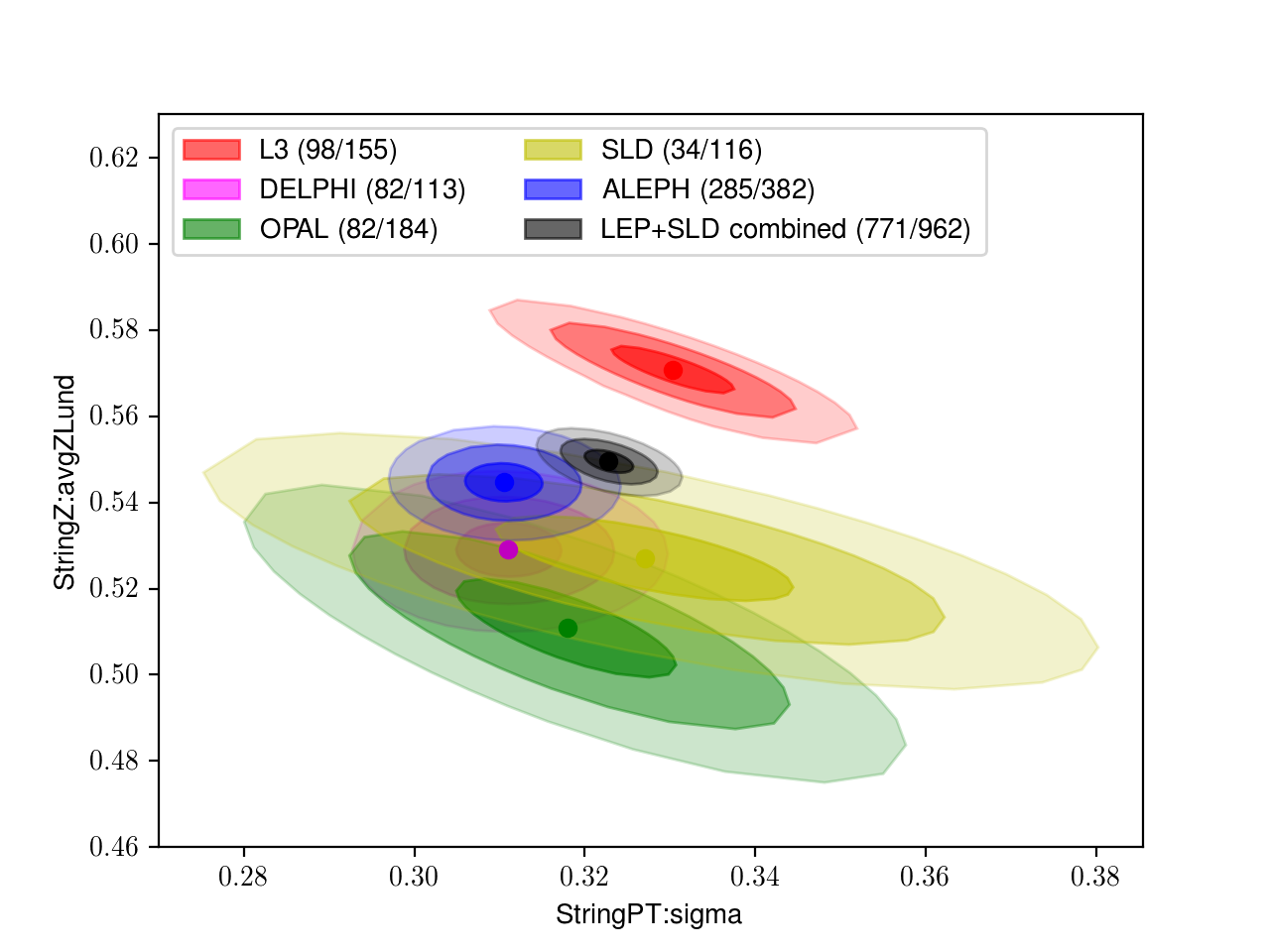
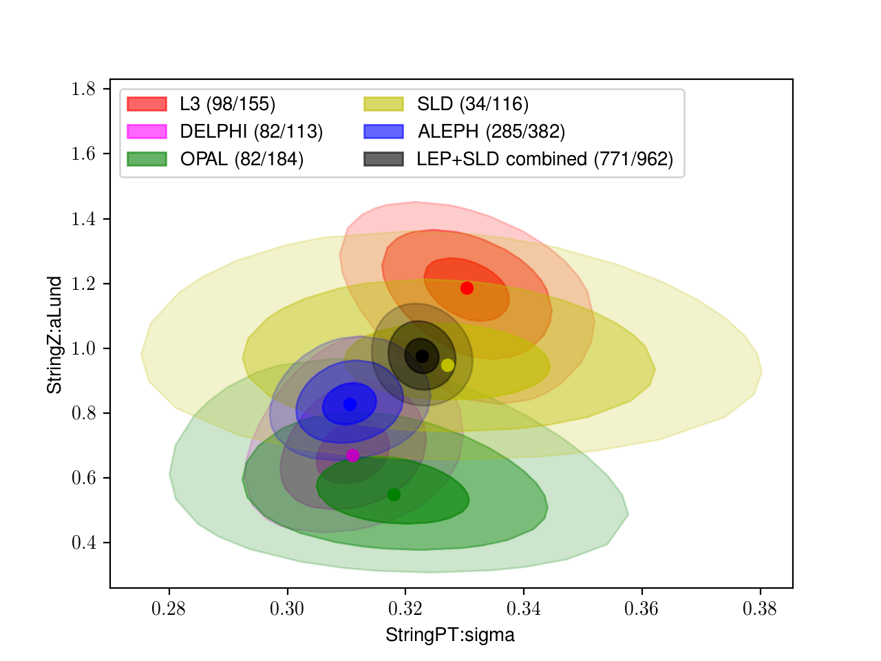
Figure 3: Results of tunes performed separately to all of the measurements from a given experiment; Aleph (blue), Delphi (magenta), L3 (red), Opal (green), Sld (yellow) and COMBINED (gray). The contours corresponding to one, two and three sigma deviations are also shown.

We show the possible tensions in the data measured by the different experiments by making independent tunes including all of the sensitive measurements by each experiment. We performed five independent tunes corresponding to the individual measurements by Aleph, Delphi, L3, Opal and Sld and display these results in Fig. 3. We can see that the tunes to Aleph, Delphi, Opal and Sld are in agreement regarding the obtained value of StringZ:avgZLund contrarily to L3. Due to the correlations between the $a$ and the $b$ (or $<z_{\rho}>$) parameters, we cannot say that these discrepancies in the individual best-fit points is a sign of disagreement between theoretical predictions and data, i.e. the predictions at the best-fit point will agree with each other and with data.

4 QCD uncertainties

4.1 Estimating the uncertainties

Parameter	Value
StringZ:aLund	$0.5999\pm 0.2$
StringZ:avgZLund	$0.5278^{+0.027}_{-0.023}$
StringPT:sigma	$0.3174^{+0.042}_{-0.037}$

Table 3: Result of the single fit to all the measurements as obtained from independent optimisation to $N(=15)$ measurements. The quoted errors correspond to the $68\%$ CL uncertainty on the fit.

The QCD uncertainties can be split into two categories: perturbative related to parton showers and non-perturbative related to the hadronisation model parameters. The uncertainties on parton showering within Pythia8 were estimated using the automatic method developed in [38]. The uncertainty in this case is determined by variation of the central renormalisation scale by a factor of $2$ in two directions with a full NLO recompensation terms. Furthermore, this framework can allow for variations of the non-singular terms in the DGLAP splitting kernels. We notice that these variations give, in most of the cases, very small uncertainties and, therefore, will be neglected.

On the non-perturbative side, the Professor toolkit allows to estimate uncertainties on the fitted parameters through the eigentunes method which diagonalises the $\chi^{2}$ covariance matrix around the best-fit point. Then, it uses variations along the principal directions (eigenvectors) in the space of the optimised parameters to construct a set of $2\cdot N_{\textrm{params}}$ variations. However, the resulting eigentunes are found to provide small uncertainties which cannot be interpreted as a conservative. Therefore, we will devise a new method.

The new method consist of making a new tuning where we use $N$ different measurements to get $N$ best-fit points. We then take the $68\%$ CL errors on the parameters to be our estimate of the uncertainty (we exclude observables with little or no sensitivity on our parameters). The results of these fits along with their $68\%$ CL errors are shown in Table 3. To get a comprehensive estimate of the uncertainty bands from the $68\%$ CL errors on the model parameters, we consider all the possible variations; there are $N_{\mathrm{var}}=3^{3}-1=26$ variations. There are, however, some variations which don’t give significant impact on the predicted spectra. We have checked that there are ten variations (including the nominal tune) meaningful variations.

4.2 Impact on Dark Matter Spectra and Fits

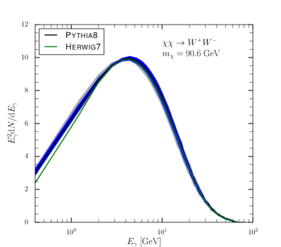
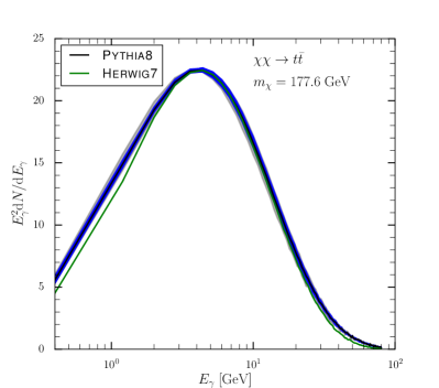
Figure 4: Photon energy distribution for dark matter annihilation into $W^{+}W^{-}$ with $m_{\chi}=90.6$ GeV (left) and into $t\bar{t}$ with $m_{\chi}=177.6$ GeV (right). In the two cases, the result corresponding to the new tune is shown in black line. Both the uncertainties from parton showering (gray bands) and from hadronisation (blue bands) are shown. Predictions from Herwig7 are shown as a gray solid line.

In this subsection, we show the results of the of QCD fragmentation function, parton shower uncertainties on the photon spectra of two representative DM annihilation channels: $W^{+}W^{-}$ and $t\bar{t}$. We do not perform a full analysis to determine the best fit of the GCE, using PASS8 data performed in the pMSSM [13] but only show qualitatively the size of the uncertainties. As the best-fit point will be certainly affected by these uncertainties, we postpone this to a future study. In the analysis of [13], the best-fit was found for two neutralino masses, i.e $m_{\chi}=90.6$ GeV and $m_{\chi}=177.6$ GeV corresponding to the $W^{+}W^{-}$ and $t\bar{t}$ DM annihilation channels respectively. These results are shown in Fig. 4 for $m_{\chi}=90.6$ GeV in the $W^{+}W^{-}$ channel (left panel) and for $m_{\chi}=177.6$ GeV in the $t\bar{t}$ channel (right panel) with the new tune (black line) and the Herwig prediction (green line). The bands show the Pythia parton-shower (gray bands) and hadronisation (blue bands) uncertainties. We can see that the predictions from Pythia and Herwig agree very well except for $E_{\gamma}\leqslant 2~{}$GeV where differences can reach about $21\%$ for $E_{\gamma}\sim 0.4$ GeV. One can see that the uncertainties can be important for both channels particularly, in the peak region which corresponds to energies where the photon excess is observed in the galactic center region. Indeed, combining them in quadrature assuming the different type of uncertainties are uncorrelated, they can go from few percents where the GCE lies to about 70% in the high energy bins. Furthermore hadronisation uncertainties are the dominant ones around the peak of the photon spectrum. The parton showering uncertainties can change the peak of the energy spectra and are the main source of uncertainties while moving away toward the edges of the spectra.

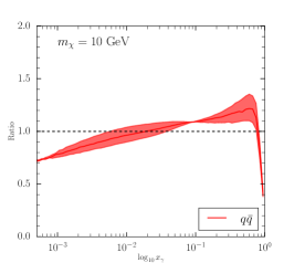
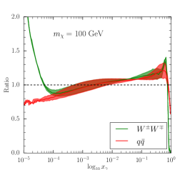
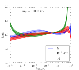
Figure 5: Photon spectra obtained using our tune normalized to the results of [24] for $m_{\chi}=10$ GeV (left pane), $m_{\chi}=100$ GeV (center pane) and $m_{\chi}=1000$ GeV (right pane). The spectra are shown for DM annihilation into $q\bar{q}$ (red), $W^{\pm}W^{\mp}$ (green) and $t\bar{t}$ (blue). The dashed bands show the QCD uncertainties on the parameters of the Lund fragmentation function.

5 Public Data on Zenodo

The impact of the QCD uncertainties on the particle spectra from DM annihilation were produced in the form of tables which can be found in Zenodo [51]. We have produced tables for five stables final states; gamma-rays, positrons, electron anti-neutrinos, muon anti-neutrinos and tau anti-neutrinos – the work on the spectra of anti-protons is in progress [52] –. The calculations were done for various DM annihilation channels; $\chi\chi\to e^{+}e^{-},\mu^{+}\mu^{-},\tau^{+}\tau^{-},q\bar{q}(q=u,d,s),c\bar{c},b\bar{b},t\bar{t},W^{+}W^{-},ZZ,gg,~{}\mathrm{and}~{}hh$. We covered DM masses from $5$ GeV to $100~{}$GeV. For each final state, and annihilation channel, there are twelve tables which are provided in zip format. The notation of the different tables is given below:

• The table corresponding to the central prediction for the spectra is denoted by ’AtProduction-Hadronization1-$TYPE.dat’ with $TYPE=Nuel, Numu, Nuta, Ga, and Positrons refers to the three flavours of anti-neutrinos, gamma-rays and positrons respectively.

• There are nine tables corresponding to the different variations of the light quark fragmentation function’s parameters. These tables are denoted by ’AtProduction-Hadronization$h-$TYPE.dat’ with h=2,..,10.

• The particle spectra corresponding to the variations of the shower evolution scale ($\mu_{R}$) are denoted by ’AtProduction-Shower-Var$s-$TYPE.dat’ with s=1,2 corresponds to $\mu_{R}/2$ and $2\mu_{R}$.

We stress that the uncertainties from parton shower and hadronisation were taken to be uncorrelated (more details on the generation of the spectra can be found in [35]).

Finally, we have compared our predictions to the results of the PPPC4DMID. We show the comparison between our predictions and the results of the PPPC4DMID in the photon spectra for three DM masses; $m_{\chi}=10,100$ and $1000$ GeV. We have chosen three final states, i.e $q\bar{q},q=u,d,s$, $W^{\pm}W^{\mp}$ and $t\bar{t}$. We can see that the differences between our results and the predictions of the Cookbook can be very important, particularly in the edges of the distributions (small $x_{\gamma}$ and large $x_{\gamma}$). As these differences cannot be accounted for by QCD uncertainties (shown as dashed bands in Fig. 5), we urge to use the updated predictions from this study.

6 Conclusions

In this talk, we discussed the study of the QCD uncertainties on particle spectra from DM annihilation which we studied for the first time in [35]. We demonstrated that the relative differences between the predictions of different multi-purposes MC event generators (Herwig 7.1.3, Pythia 8.235 and Sherpa 2.2.5) cannot be used to define a conservative estimate of QCD uncertainties particularly in the bulk of the spectra. We studied a complementary approach by using the same modeling paradigm (Pythia8) to define parametric variations taking the default Monash tune as our baseline and performed several retunings using data from LEP. Next, we show quantitatively the impact of the QCD uncertainties on the spectra of gamma-rays from DM annihilation in two benchmark points in the pMSSM. Full data tables which can be used to update those in the PPPC4DMID are public now on Zenodo and can be found in http://doi.org/10.5281/zenodo.3764809.

References

- [1] G. Bertone, D. Hooper and J. Silk, Phys. Rept. 405, 279 (2005) doi:10.1016/j.physrep.2004.08.031 [hep-ph/0404175].
- [2] P. A. R. Ade et al. [Planck Collaboration], Astron. Astrophys. 594 (2016) A13 doi:10.1051/0004-6361/201525830 [arXiv:1502.01589 [astro-ph.CO]].
- [3] W. B. Atwood et al. [Fermi-LAT Collaboration], Astrophys. J. 697 (2009) 1071 doi:10.1088/0004-637X/697/2/1071 [arXiv:0902.1089 [astro-ph.IM]].
- [4] M. Aguilar et al. [AMS Collaboration], Phys. Rev. Lett. 110 (2013) 141102. doi:10.1103/PhysRevLett.110.141102
- [5] M. G. Aartsen et al. [IceCube Collaboration], Phys. Rev. Lett. 110 (2013) no.13, 131302 doi:10.1103/PhysRevLett.110.131302 [arXiv:1212.4097 [astro-ph.HE]].
- [6] K. Griest and D. Seckel, Phys. Rev. D 43 (1991) 3191. doi:10.1103/PhysRevD.43.3191
- [7] L. Bergström, Rept. Prog. Phys. 63 (2000) 793 doi:10.1088/0034-4885/63/5/2r3 [hep-ph/0002126].
- [8] M. J. Baker et al., JHEP 1512 (2015) 120 doi:10.1007/JHEP12(2015)120 [arXiv:1510.03434 [hep-ph]].
- [9] O. Catà, A. Ibarra and S. Ingenhütt, Phys. Rev. Lett. 117 (2016) no.2, 021302 doi:10.1103/PhysRevLett.117.021302 [arXiv:1603.03696 [hep-ph]].
- [10] H. Azri, A. Jueid, C. Karahan and S. Nasri, Phys. Rev. D 102 (2020) no.8, 084036 doi:10.1103/PhysRevD.102.084036 [arXiv:2007.09681 [hep-ph]].
- [11] M. Ajello et al. [Fermi-LAT Collaboration], Astrophys. J. 819 (2016) no.1, 44 doi:10.3847/0004-637X/819/1/44 [arXiv:1511.02938 [astro-ph.HE]].
- [12] L. Goodenough and D. Hooper, [arXiv:0910.2998 [hep-ph]].
- [13] A. Achterberg, M. van Beekveld, S. Caron, G. A. Gómez-Vargas, L. Hendriks and R. Ruiz de Austri, JCAP 12 (2017), 040 doi:10.1088/1475-7516/2017/12/040 [arXiv:1709.10429 [hep-ph]].
- [14] A. Butter, S. Murgia, T. Plehn and T. M. P. Tait, Phys. Rev. D 96 (2017) no.3, 035036 doi:10.1103/PhysRevD.96.035036 [arXiv:1612.07115 [hep-ph]].
- [15] G. Bertone, F. Calore, S. Caron, R. Ruiz, J. S. Kim, R. Trotta and C. Weniger, JCAP 04 (2016), 037 doi:10.1088/1475-7516/2016/04/037 [arXiv:1507.07008 [hep-ph]].
- [16] A. Achterberg, S. Amoroso, S. Caron, L. Hendriks, R. Ruiz de Austri and C. Weniger, JCAP 08 (2015), 006 doi:10.1088/1475-7516/2015/08/006 [arXiv:1502.05703 [hep-ph]].
- [17] A. Metz and A. Vossen, Prog. Part. Nucl. Phys. 91 (2016) 136 doi:10.1016/j.ppnp.2016.08.003 [arXiv:1607.02521 [hep-ex]].
- [18] B. Andersson, G. Gustafson, G. Ingelman and T. Sjostrand, Phys. Rept. 97 (1983), 31-145 doi:10.1016/0370-1573(83)90080-7
- [19] X. Artru and G. Mennessier, Nucl. Phys. B 70 (1974), 93-115 doi:10.1016/0550-3213(74)90360-5
- [20] J. C. Winter, F. Krauss and G. Soff, Eur. Phys. J. C 36 (2004), 381-395 doi:10.1140/epjc/s2004-01960-8 [arXiv:hep-ph/0311085 [hep-ph]].
- [21] B. R. Webber, Nucl. Phys. B 238 (1984), 492-528 doi:10.1016/0550-3213(84)90333-X
- [22] A. Buckley et al., Phys. Rept. 504 (2011) 145 doi:10.1016/j.physrep.2011.03.005 [arXiv:1101.2599 [hep-ph]].
- [23] J. A. R. Cembranos, A. de la Cruz-Dombriz, V. Gammaldi, R. A. Lineros and A. L. Maroto, JHEP 1309 (2013) 077 doi:10.1007/JHEP09(2013)077 [arXiv:1305.2124 [hep-ph]].
- [24] M. Cirelli et al., JCAP 1103 (2011) 051 Erratum: [JCAP 1210 (2012) E01] doi:10.1088/1475-7516/2012/10/E01, 10.1088/1475-7516/2011/03/051 [arXiv:1012.4515 [hep-ph]].
- [25] A. Buckley, H. Hoeth, H. Lacker, H. Schulz and J. E. von Seggern, Eur. Phys. J. C 65 (2010), 331-357 doi:10.1140/epjc/s10052-009-1196-7 [arXiv:0907.2973 [hep-ph]].
- [26] A. Buckley, J. Butterworth, L. Lonnblad, D. Grellscheid, H. Hoeth, J. Monk, H. Schulz and F. Siegert, Comput. Phys. Commun. 184 (2013), 2803-2819 doi:10.1016/j.cpc.2013.05.021 [arXiv:1003.0694 [hep-ph]].
- [27] P. Z. Skands, Phys. Rev. D 82 (2010), 074018 doi:10.1103/PhysRevD.82.074018 [arXiv:1005.3457 [hep-ph]].
- [28] S. Platzer and S. Gieseke, Eur. Phys. J. C 72 (2012), 2187 doi:10.1140/epjc/s10052-012-2187-7 [arXiv:1109.6256 [hep-ph]].
- [29] A. Karneyeu, L. Mijovic, S. Prestel and P. Z. Skands, Eur. Phys. J. C 74 (2014), 2714 doi:10.1140/epjc/s10052-014-2714-9 [arXiv:1306.3436 [hep-ph]].
- [30] N. Fischer, S. Gieseke, S. Plätzer and P. Skands, Eur. Phys. J. C 74 (2014) no.4, 2831 doi:10.1140/epjc/s10052-014-2831-5 [arXiv:1402.3186 [hep-ph]].
- [31] P. Skands, S. Carrazza and J. Rojo, Eur. Phys. J. C 74 (2014) no.8, 3024 doi:10.1140/epjc/s10052-014-3024-y [arXiv:1404.5630 [hep-ph]].
- [32] N. Fischer, S. Prestel, M. Ritzmann and P. Skands, Eur. Phys. J. C 76 (2016) no.11, 589 doi:10.1140/epjc/s10052-016-4429-6 [arXiv:1605.06142 [hep-ph]].
- [33] J. Kile and J. von Wimmersperg-Toeller, [arXiv:1706.02242 [hep-ex]].
- [34] D. Reichelt, P. Richardson and A. Siodmok, Eur. Phys. J. C 77 (2017) no.12, 876 doi:10.1140/epjc/s10052-017-5374-8 [arXiv:1708.01491 [hep-ph]].
- [35] S. Amoroso, S. Caron, A. Jueid, R. Ruiz de Austri and P. Skands, JCAP 1905 (2019) 007 doi:10.1088/1475-7516/2019/05/007 [arXiv:1812.07424 [hep-ph]].
- [36] T. Sjöstrand et al., Comput. Phys. Commun. 191 (2015) 159 doi:10.1016/j.cpc.2015.01.024 [arXiv:1410.3012 [hep-ph]].
- [37] S. Catani, B. R. Webber and G. Marchesini, Nucl. Phys. B 349 (1991), 635-654 doi:10.1016/0550-3213(91)90390-J
- [38] S. Mrenna and P. Skands, Phys. Rev. D 94 (2016) no.7, 074005 doi:10.1103/PhysRevD.94.074005 [arXiv:1605.08352 [hep-ph]].
- [39] J. Bellm, S. Gieseke, D. Grellscheid, S. Plätzer, M. Rauch, C. Reuschle, P. Richardson, P. Schichtel, M. H. Seymour and A. Siódmok, et al. Eur. Phys. J. C 76 (2016) no.4, 196 doi:10.1140/epjc/s10052-016-4018-8 [arXiv:1512.01178 [hep-ph]].
- [40] S. Platzer and S. Gieseke, JHEP 01 (2011), 024 doi:10.1007/JHEP01(2011)024 [arXiv:0909.5593 [hep-ph]].
- [41] T. Gleisberg, S. Hoeche, F. Krauss, M. Schonherr, S. Schumann, F. Siegert and J. Winter, JHEP 02 (2009), 007 doi:10.1088/1126-6708/2009/02/007 [arXiv:0811.4622 [hep-ph]].
- [42] S. Schumann and F. Krauss, JHEP 03 (2008), 038 doi:10.1088/1126-6708/2008/03/038 [arXiv:0709.1027 [hep-ph]].
- [43] T. Sjostrand, S. Mrenna and P. Z. Skands, JHEP 05 (2006), 026 doi:10.1088/1126-6708/2006/05/026 [arXiv:hep-ph/0603175 [hep-ph]].
- [44] S. Gieseke, P. Stephens and B. Webber, JHEP 12 (2003), 045 doi:10.1088/1126-6708/2003/12/045 [arXiv:hep-ph/0310083 [hep-ph]].
- [45] P. Abreu et al. [DELPHI], Z. Phys. C 73 (1996), 11-60 doi:10.1007/s002880050295
- [46] F. James and M. Roos, Comput. Phys. Commun. 10 (1975), 343-367 doi:10.1016/0010-4655(75)90039-9
- [47] P. Skands, doi:10.1142/9789814525220_0008 [arXiv:1207.2389 [hep-ph]].
- [48] A. Heister et al. [ALEPH], Eur. Phys. J. C 35 (2004), 457-486 doi:10.1140/epjc/s2004-01891-4
- [49] R. Barate et al. [ALEPH], Phys. Rept. 294 (1998), 1-165 doi:10.1016/S0370-1573(97)00045-8
- [50] D. Buskulic et al. [ALEPH], Z. Phys. C 69 (1996), 365-378 doi:10.1007/BF02907417
- [51] S. Amoroso, S. Caron, A. Jueid, R. Ruiz de Austri, P. Skands, [Data set] Zenodo, http://doi.org/10.5281/zenodo.3764809
- [52] S. Caron, A. Jueid, R. Ruiz de Austri, P. Skands, to be published (2021)