Nucleon structure and spin effects in elastic hadron scattering

Abstract

Soft diffraction phenomena in elastic nucleon scattering are considered from the viewpoint of the spin dependence of the interaction potential. Spin-dependent pomeron effects are analyzed for elastic $pp$ scattering, spin-dependent differential cross sections and spin correlation parameters are calculated. The spin correlation parameter $A_{N}$ is examined on the basis of experimental data from $\sqrt{s}=4.9\ GeV$ up to $23.4\$GeV in the framework of the extended High Energy Generalized Structure (HEGS) model. It is shown that the existing experimental data of proton-proton and proton-antiproton elastic scattering at high energy in the region of the diffraction minimum and at large momentum transfer give the support of the existence of the energy-independent part of the hadron spin flip amplitude.

1 Introduction

Determination of the structure of the hadron scattering amplitude is an important task for both theory and experiment. Perturbative Quantum Chromodynamics cannot be used in calculation of the real and imaginary parts of the scattering amplitude in the diffraction range. A worse situation holds for spin-flip parts of the scattering amplitude in the domain of small transfer momenta. On the one hand, the usual representation tells us that the spin-flip amplitude dies at superhigh energies, and on the other hand, we have different nonperturbative models which lead to a nondyig spin-flip amplitude at superhigh energies [4, 1, 2, 3].

The researches into the spin-dependent structure of the hadron scattering amplitude are important for various tasks. On the one hand, the spin amplitudes constitute the spin portrait of the nucleon. Without knowing their energy and momentum transfer dependence, it is impossible to understand spin observable of nucleon scattering of nuclei. Such knowledge is also needed for the studies of very subtle effects, such as some attempts to search for a null-test signal of T-invariance violation under P-parity conservation in a $pd$ double polarization collision at SPD NICA energies [5]. Parity violation in the interaction of longitudinally polarized protons or deuterons with an unpolarized target have been discussed in [6], and the estimates of the P-odd asymmetry in nucleon-nucleon scattering in the NICA energy range were reported in [7]. This is especially important for future fixed-target experiments at LHC, in which $pp$, $pd$ and $pA$ collisions can be performed at $\sqrt{s_{NN}}=115$ GeV as well as $Pbp$ and $PbA$ collisions at $\sqrt{s_{NN}}=72$ GeV.

The study of elastic scattering requires knowledge of the properties of the pomeron, the object determining the interaction of hadrons in elastic and exclusive processes. In this case, the study of the structure and spin properties of both the hadron and the pomeron acquires a special role [8]. The vacuum $t$-channel amplitude is usually associated with two-gluon exchange in QCD [9]. The properties of the spinless pomeron were analyzed on the basis of a QCD model, by taking into account the non-perturbative properties of the theory [10, 11]. Now we recognize that the research into the pomeron exchange requires not only a pure elastic process but also many physical processes involving electroweak boson exchanges [12]. There are two approaches to the pomeron, the ”soft” pomeron built of multiperipheral hadron exchanges and a more current perturbative-QCD ”hard” pomeron built of the gluon-ladder.

The spin structure of the pomeron is still an unresolved question in diffractive scattering of polarized particles. There have been many observations of spin effects at high energies and at fixed momentum transfers [13, 14]; several attempts to extract the spin-flip amplitude from the experimental data show that the ratio of spin-flip to spin-nonflip amplitudes can be non-negligible and may be independent of energy [15, 16].

It is generally believed, based on calculations of the simplest QCD diagrams, that the spin effects decrease as an inverse power of the center-of-mass energy and that the pomeron exchange does not lead to appreciable spin effects in the diffraction region at super-high energies. Complete calculations of the full set of helicity scattering amplitudes in the diffraction region cannot be carried out presently since they require extensive treatment of confinement and contributions from many diagrams. Semi-phenomenological models, however, have been developed with parameters which are expected to be fixed with the aid of data from experiments. There is a specific features of model approaches to the description of spin correlations parameters. They can be divided into two classes - low energy and high energy. In the region of low energies there is a wide range of experimental data. To describe the data quantitatively the models used pure phenomenological approaches like [17] or obtained some qualitative descriptions of the data in some theoretical approaches [18]. Above $\sqrt{s}=10$ GeV the number of experimental data essentially decreases, practically gives only the values of the analysing power $A_{N}(s,t)$. The description of such data was presented in the old famous Bourrelly-Soffer model [4] and recently in the model with a huge number of free parameters [20]. However, such models do not take into account in the analysis the data at $\sqrt{s}<13$ GeV.

Some models predict non-zero spin effects as $s\to\infty$ and $|t|/s\to 0$. In these studies, the spin-flip amplitudes, which lead to weakly altered spin effects with increasing energy, are connected with the structure of hadrons and their interactions at large distances [19, 1]. In [19], the spin-dependence of the pomeron term is constructed within model rotation of matter inside the proton. This approach is based on Chou and Yang’s concept of hadronic current density [21]. This picture can be related with the spin effects determined by higher-order $\alpha_{s}$ contributions in the framework of PQCD.

The high energy two-particle amplitude determined by pomeron exchange can be written in the form:

$$T(s,t)=is\ IP(s,t)V_{h_{1}h_{1}IP}^{\mu}\otimes V^{h_{2}h_{2}spIP}_{\mu}.$$ (1)

Here $IP(s,t)$ is a function caused by a pomeron with a weak energy dependence $\sim(\ln{s})^{n}$ and $V_{\mu}^{hhIP}$ are the pomeron-hadron vertices. The perturbative calculation of the pomeron coupling structure is rather difficult, and the non-perturbative contributions are important for momentum transfers of a few $\,{\rm(GeV}/c)^{2}$. The situation changes dramatically when large-distance loop contributions are considered, which leads to a more complicated spin structure of the pomeron coupling. As a result, spin asymmetries appear that have a weak energy dependence as $s\to\infty$. Additional spin-flip contributions to the quark-pomeron vertex may also have their origins in instantons, e.g. [22, 2]. Note that in the framework of the perturbative QCD, the analyzing power of hadron-hadron scattering was shown to be of the order:

$$A_{N}\ \propto\ m\alpha_{s}/\sqrt{p_{t}^{2}}$$

where $m$ is around hadron mass [23]. Hence, one would expect a large analyzing power for moderate $p_{t}^{2}$, where the spin-flip amplitudes are expected to be important for diffractive processes.

Now there are many different models to describe the elastic hadron scattering amplitude at small angles (see reviews [24, 25, 20]). They lead to different predictions of the structure of the scattering amplitude at super-high energies. The diffraction processes at very high energies, especially at LHC energies are not simple asymptotically but can display complicated features [26, 27]. Note that the interference of hadronic and electromagnetic amplitudes can give an important contribution not only at very small transfer momenta but also in the range of the diffraction minimum [8]. However, one should also know the phase of the interference of the Coulomb and hadron amplitudes at sufficiently large transfer momenta and the contribution of the hadron-spin-flip amplitude to the CNI effect [28, 19]. Now we cannot exactly calculate all contributions and find their energy dependences. But a great amount of the experimental material at low energies allows us to make complete phenomenological analyses and find the size and form of different parts of the hadron scattering amplitude. The difficulty is that we do not know the energy dependence of these amplitudes and individual contributions of the asymptotic non-dying spin-flip amplitudes.

From a modern point of view, the structure of a hadron can be described by the Generalized parton distribution (GPD) functions [29, 30, 31] combining our knowledge about the one-dimensional parton distribution in the longitudinal momentum with the impact-parameter or transverse distribution of matter in a hadron or nucleus. They allow one to obtain a 3-dimensional picture of the nucleon (nucleus) [32, 33, 34].

In the general picture, hadron-hadron processes determined by the strong interaction with the hadron spin equal to $1/2$ can be represented by some combinations of three vectors in the center of mass system. In the c.m.s. there are only two independent three-dimensional momenta. In the case of the elastic scattering, $\vec{p}_{1}=-\vec{p}_{2}$ and $\vec{p}_{3}=-\vec{p}_{4}$ Using the initial and final momenta ${\bf p}$ and $p^{\prime}$ and their unity vectors ${\bf\hat{p}}$ and ${\bf\hat{p}^{\prime}}$ , so that ${\bf\hat{p}}={\bf p}/{|\bf p}|$ and ${\bf\hat{p}}={\bf p^{\prime}}/{|\bf p}^{\prime}|$, one can obtain three independent combinations

$${\bf\hat{l}}\equiv\frac{{\bf p+p^{\prime}}}{|{\bf p+p^{\prime}}|};\ \ \ {\bf\hat{q}}\equiv\frac{{\bf p-p\prime}}{|{\bf p-p\prime}|};\ \ \ {\bf\hat{n}}\equiv\frac{{\bf p\times p^{/}}}{|{\bf p\times p^{/}}|}.$$

The vectors ${\bf\hat{l}}$, ${\bf\hat{q}}$, ${\bf\hat{n}}$ and spin-vectors ${\hat{\sigma_{1}}}$ and ${\hat{\sigma_{2}}}$ create eight independent scalars [35] $({\hat{\sigma_{1}}}{\bf\hat{n}})({\hat{\sigma_{2}}}{\bf\hat{n}})\ \ \$, ${\hat{\sigma_{1}}}{\bf\hat{n}}+{\hat{\sigma_{2}}}{\bf\hat{n}}\ \ \$, ${\hat{\sigma_{1}}}{\bf\hat{n}}-{\hat{\sigma_{2}}}{\bf\hat{n}}\ \ \$, $({\hat{\sigma_{1}}}{\bf\hat{I}})({\hat{\sigma_{2}}}{\bf\hat{I}})\ \ \$, $({\hat{\sigma_{1}}}{\bf\hat{q}})\times({\hat{\sigma_{2}}}{\bf\hat{q}})\ \ \$, $({\hat{\sigma_{1}}}{\bf\hat{q}})({\hat{\sigma_{2}}}{\bf\hat{I}})\ \ \$, $({\hat{\sigma_{1}}}{\bf\hat{I}})({\hat{\sigma_{2}}}{\bf\hat{q}})\ \ \$, $[{\hat{\sigma_{1}}}{\hat{\sigma_{2}}}]{\bf\hat{n}}$.

The main experimental data show the conservation of time parity, charge conjugation, and space parity in the strong interaction processes. Then, under time inverse ${\hat{\sigma_{1}}}$ changes to $-{\hat{\sigma_{1}}}$, and ${\bf\hat{q}}\rightarrow{\bf\hat{q}}$, ${\bf\hat{n}}\rightarrow-{\bf\hat{n}}\ \ \$, ${\bf\hat{I}}\rightarrow-{\bf\hat{I}}$, the combinations $[{\hat{\sigma_{1}}}{\hat{\sigma_{2}}}]{\bf\hat{n}}\ \ \$ and $({\hat{\sigma_{1}}}{\bf\hat{q}})({\hat{\sigma_{2}}}{\bf\hat{I}})\ \ \$, $({\hat{\sigma_{1}}}{\bf\hat{I}})({\hat{\sigma_{2}}}{\bf\hat{q}})$ have to be removed as a result of the time parity conservation. If the interacting particles are identical, as in the case of the proton-proton elastic scattering, their combinations should not be changed when replacing one particle by another. As a result, the scattering amplitude is

$$\phi(s,t))=\phi_{1}(s,t) + \phi_{2}(s,t)({\sigma_{1}}\cdot{\bf{\hat{n}}})({\sigma_{2}}\cdot{\bf{\hat{n}}})+\phi_{3}(s,t)({\sigma_{1}}\cdot{\bf\hat{n}}+{\sigma_{2}}\cdot\bf{\hat{n}})$$ (2)

$$+ \phi_{4}(s,t)({\sigma_{1}}\cdot{\bf\hat{q}})({\sigma_{2}}\cdot{\bf\hat{q}})+\phi_{5}(s,t)({\sigma_{1}}\cdot{\bf\hat{l}})({\sigma_{2}}\cdot\bf{\hat{l}}),$$

The amplitude corresponds to the spin-dependent interaction potential. It can be taken as a Born term of scattering processes. The Born term of the amplitude in the transfer momentum representation can be obtained by the corresponding amplitudes in the impact parameter representation

$$\phi(s,b)\ =-\frac{1}{2\pi}\ \int\ d^{2}q\ e^{i\vec{b}\cdot\vec{q}}\ \phi^{\rm Born}_{h}(s,q^{2})\,,$$ (3)

The corresponding amplitude is connected to the interaction potential in the position representation. Using the standard Fourier transform [36] of the potential $V(\vec{r})$, one can obtain the Born term of the scattering amplitude. If the potentials $V(\vec{r})=V_{1}(\vec{r})+V_{5}(\vec{r})$ are assumed to have a Gaussian form

$$V_{1,5}(\rho,z)\sim\ \int_{-\infty}^{\infty}e^{-B\ r^{2}}\ dz\ =\ \frac{\sqrt{\pi}}{\sqrt{B}}e^{-B\ \rho^{2}},$$

in the first Born approximation $\phi^{h}_{1}$ and $\hat{\phi_{h}}^{5}$ will have the same form

$$\phi^{h}_{1}(s,t)\sim\int_{0}^{\infty}\ \rho\ d\rho\ J_{0}(\rho\Delta)e^{-B\ \rho^{2}}\ =\ e^{-B\Delta^{2}},$$ (4)

$$\phi^{h}_{5}(s,t)\sim\int_{0}^{\infty}\ \rho^{2}\ d\rho\ J_{1}(\rho\Delta)\ e^{\chi_{0}(s,\rho)}\ e^{-B\ \rho^{2}}\ =\ q\ \ B\ e^{-B\Delta^{2}}.$$ (5)

In this special case, therefore, the spin-flip and “residual”spin-non-flip amplitudes are indeed with the same slope [37].

The first observation that the slopes do not coincide was made in [38]. It was found from the analysis of the $\pi^{\pm}p\rightarrow\ \pi^{\pm}p$ and $pp\rightarrow\ pp$ reactions at $p_{L}\ =\ 20\div 30\ GeV/c$ that the slope of the “residual” spin-flip amplitude is about twice as large as the slope of the spin-non flip amplitude. This conclusion can also be obtained from the phenomenological analysis carried out in [17] for spin correlation parameters of the elastic proton-proton scattering at $p_{L}\ =\ 6\ GeV/c$.

The model-dependent analysis based on all the existing experimental data of the spin-correlation parameters above $p_{L}\ \geq\ 6\ GeV$ allows us to determine the structure of the hadron spin-flip amplitude at high energies and to predict its behavior at superhigh energies [39] This analysis shows that the ratios $Re\ \phi^{h}_{5}(s,t)/(\sqrt{|t|}\ Re\ \phi^{h}_{1}(s,t))$ and $Im\ \phi^{h}_{5}(s,t)/(\sqrt{|t|}\ Im\ \phi^{h}_{1}(s,t))$ depend on $\ s$ and $t$. At small momentum transfers, it was found that the slope of the “residual” spin-flip amplitudes is approximately twice the slope of the spin-non flip amplitude [40].

The electromagnetic current of a nucleon is

$$J_{\mu}(P^{{}^{\prime}},s^{{}^{\prime}};P,s)=\bar{u}(P^{{}^{\prime}},s^{{}^{\prime}})\Lambda_{\mu}(q,P)u(P,s)=\bar{u}(P^{{}^{\prime}},s^{{}^{\prime}})(\gamma_{\mu}F_{1}(q^{2})+\frac{1}{2M}i\sigma_{\mu\nu}q_{\nu}F_{2}(q^{2}))u(P,s),$$ (6)

where $P,s,(P^{{}^{\prime}},s^{{}^{\prime}})$ are the four-momentum and polarisation of the incoming (outgoing) nucleon, and $q=P^{{}^{\prime}}-P$ is the momentum transfer. The quantity $\Lambda_{\mu}(q,P)$ is the nucleon-photon vertex.

If the potential has the spherical symmetry, the Born amplitude can be calculated as

$$\phi_{B}(t)=g/q\int_{0}^{\infty}r\ sin(qr)V(\vec{r})\ dr.$$ (7)

or in the impact parameter representation

$$\phi_{B}(b)=\frac{1}{4\Pi}\int_{0}^{\infty}rV(\sqrt{(z^{2}+b^{2})})\ dr.$$ (8)

There are some different forms of the unitarization procedures [41, 42]. One of them is the standard eikonal representation, where the Born term of the scattering amplitude in the impact parameter representation takes the eikonal phase and the total scattering amplitude is represented as

$$\phi(s,t)=\frac{is}{2\pi}\int_{0}^{\infty}[1-\exp{(-\chi({\bf b})}]\exp{(-i{\bf{q\cdot b}})}d^{2}{\bf{b}}.$$ (9)

If the terms are taken into account to first order in the spin-dependent eikonals of the spin-dependent eikonal amplitude, where the eikonal function $\chi(\bf{b})$ is a sum of the spin-independent central term $\chi_{si}$, spin-orbit term - $\chi_{ls}$, and spin-spin term $\chi_{ss}$, separate spin-dependent amplitudes are written as follows:

$$\phi_{1s}(s,t) = is\int bdbJ_{0}(bq)[1-\exp{(-\chi_{si}(b))}];$$ (10)

$$\phi_{2s}(s,t) = is\int b^{2}dbJ_{1}(bq)\exp{(-\chi_{si}(b))}\chi_{ls}(b);$$ (11)

$$\phi_{3s}(s,t) = s\int bdbJ_{0}(bq)\exp{(-\chi_{si}(b))}\chi_{ss}(b).$$ (12)

Using ordinary relations (see, for example, [43]), we can obtain helicity amplitudes for small scattering angles and high energies:

$$\phi_{1}(s,t) = \phi_{1s}(s,t)-\phi_{2s}(s,t);\ \ \ \phi_{2}(s,t)=2\phi_{2s}(s,t);$$ (13)

$$\phi_{3}(s,t) = \phi_{1s}(s,t)+\phi_{2s}(s,t);\ \ \ \phi_{4}(s,t)=0;\ \ \ \phi_{5}(s,t)=i\phi_{3s}(s,t).$$

The scattering amplitude of charged hadrons is represented as a sum of the hadronic and electromagnetic amplitudes $\phi_{tot}=\phi^{em}+\phi^{h}$. The electromagnetic amplitude can be calculated in the framework of QED. In the one-photon approximation, we have [44, 45]

$$\phi^{em}_{1} = \alpha[f_{1}^{2}(t)(\frac{s-2m^{2}}{t}+\frac{m^{2}}{2p^{2}})-2f_{1}(t)f_{2}(t)-\frac{1}{2}f_{2}^{2}(t)(1-\frac{t}{4p^{2}})];$$ (14)

$$\phi^{em}_{2} = \alpha[f_{1}^{2}(t)\frac{m^{2}}{2p^{2}}-f_{1}(t)f_{2}(t)+\frac{f_{2}^{2}(t)}{4m^{2}}(s-2m^{2}+\frac{ts}{8p^{2}})];$$

$$\phi^{em}_{3} = \alpha(1+\frac{t}{4p^{2}})[f_{1}^{2}(t)\frac{s-2m^{2}}{t}+\frac{1}{2}f_{2}^{2}(t)];$$

$$\phi^{em}_{4} = -\phi^{em}_{2};$$

$$\phi^{em}_{5} = \alpha[-\frac{s(4p^{2}+t)}{t}]^{1/2}[f_{1}^{2}(t)\frac{m}{4p^{2}}-\frac{1}{2m}f_{1}(t)f_{2}(t)+\frac{t}{16mp^{2}}f_{2}^{2}(t)],$$

where $\alpha$ is the electromagnetic coupling constant, and $f_{1}(t)$ and $f_{2}(t)$ are the Dirac an Pauli form factors of the proton

$$f_{1}(t)=\frac{4m^{2}-t(1+k)}{4m^{2}-t}G_{d}\ \ \ \ f_{2}(t)=\frac{4m^{2}k}{4m^{2}-t}G_{d}$$ (15)

with $G_{d}=(1-t/0.71)^{-2}$ (t is in GeV²), and $k=1.793$ is the anomalous magnetic moment of the proton.

In the high energy approximation, we obtain:

$$\phi^{em}_{1}=\alpha f_{1}^{2}\frac{s-2m^{2}}{t},\ \ \ \phi^{em}_{3}=\phi^{em}_{1},\ \ \ \phi^{em}_{2}=\alpha\frac{f_{2}^{2}(t)}{4m^{2}}s,$$ (16)

$$\phi^{em}_{4}=-\phi^{em}_{2},\ \ \ \ \phi^{em}_{5}=\alpha\frac{s}{2m\sqrt{|t|}}f_{1}^{2},$$

The total helicity amplitudes can be written as $\phi_{i}(s,t)=\phi^{i}_{N}(s,t)+\phi^{i}_{em}(t)\exp{i\alpha\varphi(s,t)}$ [44].

The differential cross sections and spin correlation parameters are

$$\frac{d\sigma}{dt}=\frac{2\pi}{s^{2}}(|\phi_{1}|^{2}+|\phi_{2}|^{2}+|\phi_{3}|^{2}+|\phi_{4}|^{2}+4|\phi_{5}|^{2}).$$ (17)

$$A_{N}\frac{d\sigma}{dt} = -\frac{4\pi}{s^{2}}Im[(\phi_{1}+\phi_{2}+\phi_{3}-\phi_{4})\ \phi_{5}^{*}).$$ (18)

and

$$A_{NN}\frac{d\sigma}{dt} = \frac{4\pi}{s^{2}}Re[(\phi_{1}\phi_{2}^{*}-\phi_{3}\phi_{4}^{*})+2|\phi_{5}|^{2}).$$ (19)

2 Coulomb -nucleon phase factor

In [8, 4], the importance of the CNI effects in the domain of diffraction dip was pointed out. In [4], the polarization at sufficiently low (now) energies with the CNI effect but without the phase of CNI and with a simple approximation of the hadron non-flip spin amplitude was calculated. However, the authors showed for the first time that the CNI effect can be sufficiently large (up to $11\%$ at $p_{L}=280\ GeV/c$) in the region of non-small transfer momenta.

The total amplitude including the electromagnetic and hadronic forces can be expressed as

$$F(s,t)=F_{C}\exp{(i\alpha\varphi(s,t))}+F_{N}(s,t),$$ (20)

and for the differential cross sections, neglecting the terms proportional to $\alpha^{2}$, we have

$$d\sigma/dt = \pi[(F_{C}(t))^{2}\!+\!ReF_{N}^{2}(s,t)+ImF_{N}^{2}(s,t)$$

$$+ 2(ReF_{N}(s,t)F_{C}(t)cos(\alpha\varphi(t))+ImF_{N}(s,t)F_{C}(t)\ sin(\alpha\varphi(t)))]$$

with

$$\varphi(s,t)=\varphi(t)_{C}-\varphi(s,t)_{CN},$$ (22)

where $\varphi(t)_{C}$ appears in the second Born approximation of the pure Coulomb amplitude, and the term $\varphi_{CN}$ is defined by the Coulomb-hadron interference.

The quantity $\varphi(s,t)$ has been calculated and discussed by many authors. For high energies, the first results were obtained by Akhiezer and Pomeranchuk [47] for the diffraction on a black nucleus. Using the WKB approach in potential theory, Bethe [48] derived $\varphi(s,t)$ for the proton-nucleus scattering. After some treatment improving this result [50], the most important result was obtained by Locher [51] and then by West and Yennie [52]. In the framework of the Feynman diagram technique in [52], a general expression was obtained for $\varphi_{CN}(s,t)$ in the case of pointlike particles in terms of the hadron elastic scattering amplitude:

$$\varphi(s,t)=-\ln{(-t/s)}-\int^{S}_{0}\frac{dt^{{}^{\prime}}}{|t-t^{{}^{\prime}}|}\ \ (1-\frac{F_{N}(s,t^{{}^{\prime}})}{F_{N}(s,t)}).$$ (23)

If the hadron amplitude is chosen in the standard Gaussian form
$F_{N}=h\ \exp{(-B(s)q^{2}/2)}$, we can get

$$\varphi(s,t)=\mp[\ln{(-B(s)t/2)}+\gamma],$$ (24)

where $-t=q^{2}$, $B(s)/2$ is the slope of the nuclear amplitude, $\gamma$ is the Euler constant, and the upper (lower) sign corresponds to the scattering of particles with the same (opposite) charges.

The impact of the spin of scattered particles was analyzed in [8, 44] by using the eikonal approach for the scattering amplitude. Using the helicity formalism for high energy hadron scattering in [44], it was shown that at small angles, all the helicity amplitudes have the same $\varphi(s,t)$. The influence of the electromagnetic form factor of scattered particles on $\varphi_{C}$ and $\varphi_{CN}$ in the framework of the eikonal approach was examined by Islam [53] and with taking into account the hadron form factor in the simplest form by Cahn [54]. He derived for $t\rightarrow 0$ the eikonal analogue (23) and obtained the corrections

$$\varphi(s,t) = \mp[\gamma+\ln{(B(s)|t|/2)}+\ln{(1+8/(B(s)\Lambda^{2}))}$$ (25)

$$+(4|t|/\Lambda^{2})\ \ln{(4|t|/\Lambda^{2})}+2|t|/\Lambda^{2}],$$

where $\Lambda$ is a constant entering into the power dependent form factor. The recent calculation of the phase factor was carried out in [55]. The calculations of the phase factor beyond the limit $t\rightarrow 0$ were carried out in [56, 57, 58]. As a result, for the total Coulomb scattering amplitude, we have the eikonal approximation of the second order in $\alpha$

$$F_{c}(q)=F_{c}^{1B}+F_{c}^{2B}=-\frac{\alpha}{q^{2}}[\frac{\Lambda^{4}}{(\Lambda^{2}+q^{2})^{2}}][1+i\alpha(\{\ln(\frac{\lambda^{2}}{q^{2}})\ +\ \nu_{s}\}],$$ (26)

where

$$\nu_{s}=A\ln(\frac{(\Lambda^{2}+q^{2})^{2}}{\Lambda^{2}q^{2}})+B\ln(\frac{4\Lambda^{2}}{(\sqrt{(4\Lambda^{2}+q^{2}}+q)^{2}})\ +\ C,$$ (27)

The coefficients $A,B,C$ are defined in [58]. The numerical calculation shows that at small $q^{2}$ the difference between $\nu_{s}$ and $\nu_{c}$ is small, but above $q^{2}=3.10^{-2}\ GeV^{2}$, it is rapidly growing. It is clear that the solution of $\nu_{c}$ should be bounded at $-t=3.10^{-2}\ GeV^{2}$. As a result, we have a sufficiently simple form of $\nu_{s}$ up to $|t|=0.2\ GeV^{2}$. It gives us the possibility to reproduce it by a simple phenomenological form that can be used in a practical analysis of experimental data at small $t$:

$$\nu_{s}\simeq=c_{1}\log{(1+c_{2}^{2}q^{2})}+4/q^{2},$$ (28)

where the constants $c_{1}$ and $c_{2}$ are defined by the fit $\nu_{s}$, $c_{1}=0.11,\ \ \ \ c_{2}=20.$

The total phase factor is

$$\varphi(s,t)=\ln{\frac{q^{2}}{4}}+2\gamma+\frac{1}{F_{h}(s,q)}\int_{0}^{\infty}\tilde{\chi}_{c}(\rho)(1-\exp(\chi_{h}(\rho,s))J_{0}(\rho,q)d\rho,$$ (29)

with

$$\tilde{\chi}_{c}(\rho)=2\rho\ln{\rho}+2\rho\biggl{\{}K_{0}(\rho\Lambda)[1+\frac{5}{24}\Lambda^{2}\rho^{2}]+\frac{\Lambda\rho}{12}K_{1}(\rho\Lambda)[11+\frac{1}{4}\Lambda^{2}\rho^{2}]\biggr{\}}$$ (30)

The calculated $\varphi(s,t)$, Eq.(29), is an eikonal analog with taking account the hadron form factor of the expression obtained by West and Yennie [52] from the Feynman diagram.

3 Nucleon form factors and GPDs

There are various choices for the nucleon electromagnetic form factors (ff), such as the Dirac and Pauli ff, $F_{1}^{p}(t),\ \ F_{1}^{n}(t)$ and $F_{2}^{p}(t),\ \ F_{2}^{n}(t),$ the Sachs electric and magnetic ff, $G_{E}^{p}(t),\ \ G_{E}^{n}(t)$ and $G_{M}^{p}(t),\ \ G_{M}^{n}(t),$ [59].

The Dirac and Pauli form factors are obtained from a decomposition of the matrix elements of the electromagnetic (e.m.) current in linearly independent covariants made of four-momenta, $\gamma$ matrices and Dirac bispinors as follows:

$$<N|J_{\mu}^{e.m.}|N>=e\bar{u}(p^{\prime})[\gamma_{\mu}F_{1}^{N}(t)+{i\over{2m}}\sigma_{\mu\nu}(p^{\prime}-p)_{\nu}F_{2}^{N}(t)]u(p),$$

where $m$ is the nucleon mass. The electric and magnetic form factors, on the other hand, are suitable in extracting them from the experiment: $e^{-}N\rightarrow e^{-}N$ by Rosenbluch or polarization methods [61]. The four independent sets of form factors are related by

$$G_{E}^{p}(t)=F_{1}^{p}(t)+\tau^{p}F_{2}^{p}(t),\ \ \ G_{M}^{p}(t)=F_{1}^{p}(t)+F_{2}^{p}(t),$$ (31)

$$G_{E}^{n}(t)=F_{1}^{n}(t)+\tau^{n}F_{2}^{n}(t),\ \ \ G_{M}^{n}(t)=F_{1}^{n}(t)+F_{2}^{n}(t),$$

with $\tau^{p(n)}={t\over{4m_{p(n)}^{2}}}$, which can be interpreted as Fourier transformations of the distribution of magnetism and charge in the Breit frame. They satisfy the normalization conditions

$$G_{E}^{p}(0)=1;\ G_{M}^{p}(0)=1+\mu_{p};\ G^{n}_{E}(0)=0;G^{n}_{M}(0)=\mu_{n};$$

where $\mu_{p}$ and $\mu_{n}$ are the proton and neutron anomalous magnetic moments, respectively.

Since the GPD is not known a priori, one seeks for models of GPD based on general constraints on its analytic and asymptotic behavior. The calculated scattering amplitudes (cross sections) are than compared with the data to confirm, modify or reject the chosen form of the GPD.

Commonly, the form $GPDs(x,\xi,t)$ is determined through the exclusive deep inelastic processes of type $\gamma^{*}p\rightarrow Vp,$ where $V$ stands for a photon or vector meson. However, such processes have a narrow region of momentum transfer and in most models the $t$-dependence of GPDs is taken in the factorization form with the Gaussian form of the $t$-dependence. Really, this form of $GPDs(x,\xi,t)$ can not be used to build the space structure of the hadrons, as for that one needs to integrate over $t$ in a maximum wide region.

The hadron form factors are related to the $GPDs(x,\xi,t)$ by the sum rules [30]

$$F_{1}^{q}(t)=\int_{-1}^{1}dxH^{q}(x,\xi=0,t),\ \ \ \ F_{1}^{q}(t)=\int_{-1}^{1}dxH^{q}(x,\xi=0,t).$$ (32)

The integration region can be reduced to positive values of $x,~{}0<x<1$ by the following combination of non-forward parton densities [62, 63] ${\cal H}^{q}(x,t)=H^{q}(x,0,t)+H^{q}(-x,0,t)$, ${\cal E}^{q}(x,t)=E^{q}(x,0,t)+E^{q}(-x,0,t)$, providing $F^{q}_{1}(t)=\int_{0}^{1}dx{\cal H}^{q}(x,t)$, $F^{q}_{2}(t)=\int_{0}^{1}dx{\cal E}^{q}(x,t).$

The proton and neutron Dirac form factors are defined as

$$F_{1}^{p}(t)=e_{u}F_{1}^{u}(t)+e_{d}F_{1}^{d}(t),\ \ \ \ F_{1}^{n}(t)=e_{u}F_{1}^{d}(t)+e_{d}F_{1}^{u}(t),$$ (33)

where $e_{u}=2/3$ and $e_{d}=-1/3$ are the relevant quark electric charges. As a result, the $t$-dependence of the $GPDs(x,\xi=0,t)$ can be determined from the analysis of the nucleon form factors for which experimental data exist in a wide region of momentum transfer. It is a unique situation as it unites the elastic and inelastic processes.

In the limit $t\rightarrow 0$ the functions $H^{q}(x,t)$ reduce to usual quark densities in the proton:

$${\cal\ H}^{u}(x,t=0)=u_{v}(x),\ \ \ {\cal H}^{d}(x,t=0)=d_{v}(x)$$

with the integrals

$$\int_{0}^{1}u_{v}(x)dx=2,\ \ \ \int_{0}^{1}d_{v}(x)dx=1$$

normalized to the number of $u$ and $d$ valence quarks in the proton.

However, the ”magnetic” densities ${\cal E}^{q}(x,t=0)\equiv{\cal E}^{q}(x)$ cannot be directly expressed in terms of the known parton distributions; however, their normalization integrals

$$\int_{0}^{1}{\cal E}^{q}(x)dx\equiv k_{q}$$

are constrained by the requirement that the values $F_{2}^{p}(t=0)$ and $F_{2}^{n}(t=0)$ are equal to the magnetic moments of the proton and neutron, whence $k_{u}=2k_{p}+k_{n}\approx 1.673$ and $k_{u}=k_{p}+2k_{n}\approx-2.033$ follow [63]. This helps us to obtain the corresponding PDFs by analysing the magnetic form factor of the proton and neutron [64]

In [64], the $t$-dependence of GPDs in the simplest form

$${\cal{H}}^{q}(x,t)\ =q(x)_{nf}\ exp[a_{+}\ \frac{(1-x)^{2}}{x^{m}}\ t];\ \ \ {\cal{E}}^{q}(x,t)\ =q(x)_{sf}\ exp[a_{-}\ \frac{(1-x)^{2}}{x^{m}}\ t];$$ (34)

was researched. Complicated analysis of all available experimental data on the electromagnetic form factors of proton and neutron simultaneously allows one to obtain the $t$-dependence of the $GPDs(x,\xi,t)$ [65]. Different Mellin moments of GPDs give the form factors for different reactions. If the first momentum of $GPDs(x,\xi,t)$ gives the electromagnetic form factors, then the integration of the second moment of GPDs over $x$ gives the momentum-transfer representation of the so called gravitomagnetic form factors over $x,t$,

$$\int^{1}_{0}\ dx\ x\sum_{u,d}[{\cal{H}}(x,t)\pm{\cal{E}}(x,t)]=A_{h}(t)\pm B_{h}(t).$$ (35)

which are connected with the energy-momentum tensor.

Further development of the model requires careful analysis of the momentum transfer form of the GPDs and a properly chosen form of the PDFs. In Ref. [65], analysis of more than 24 different PDFs was performed. We slightly complicated the form of the GPDs in comparison with Eq.(34), but it is the simplest one compared to other works (for example, Ref. [66]):

$${\cal{H}}^{u}(x,t)=q(x)^{u}_{nf}\ e^{2a_{H}\ \frac{(1-x)^{2+\epsilon_{u}}}{(x_{0}+x)^{m}}\ t};\ \ \ {\cal{H}}^{d}(x,t)\ =q(x)^{d}_{nf}\ e^{2a_{H}(1+\epsilon_{0})(\frac{(1-x)^{2+\epsilon_{d}}}{(x_{0}+x)^{m}})\ t},$$ (36)

$${\cal{E}}^{u}(x,t)=q(x)^{u}_{fl}\ e^{2a_{E}\ \frac{(1-x)^{2+\epsilon_{u}}}{(x_{0}+x)^{m}}\ t},\ \ \ {\cal{E}}^{d}(x,t)=q(x)^{d}_{fl}\ e^{2a_{E}(1+\epsilon_{0})(\frac{(1-x)^{2+\epsilon_{d}}}{(x_{0}+x)^{m}})\ t},$$ (37)

where $q(x)^{u,d}_{fl}=q(x)^{u,d}_{nf}(1.-x)^{z_{1},z_{2}}$.

The ratio of $\mu G_{E}/G_{M}$ for the proton and neutron cases is presented in Fig. 1. Our calculations reproduce the data obtained by the polarization method quite well.

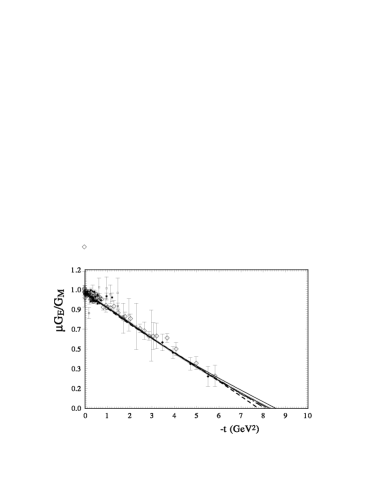
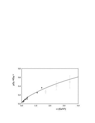
Figure 1: The model description of the ratio of the electromagnetic form factors for the proton $\mu_{p}G^{p}_{E}/G^{p}_{M}$ with different forms of PDFs [67] [left], and for the neutron $\mu_{n}G^{n}_{E}/G^{n}_{M}$ [right],.

The hadron form factors were calculated by using numerical integration

$$F_{1}(t)=\int^{1}_{0}dx[\frac{2}{3}q_{u}(x)e^{2\alpha_{H}t(1.-x)^{2+\epsilon_{u}}/(x_{0}+x)^{m}}-\frac{1}{3}q_{d}(x)e^{2\alpha_{H}t(1.-x)^{2+\epsilon_{d}}/((x_{0}+x)^{m})}]$$ (38)

and then by fitting these integral results with the standard dipole form with some additional parameters for $F_{1}(t)$, $F_{1}(t)=1/(1+q/a_{1}+q^{2}/a_{2}^{2}+q^{3}/a_{3}^{3})^{2})$. The matter form factor

$$A(t)=\int^{1}_{0}x\ dx[q_{u}(x)e^{2\alpha_{H}t(1.-x)^{2+\epsilon_{u}}/(x_{0}+x)^{m}}+q_{d}(x)e^{2\alpha_{H}t(1.-x)^{2+\epsilon_{d}}/((x_{0}+x)^{m})}]$$ (39)

is fitted by the simple dipole form $A(t)=\frac{\Lambda^{4}}{(\Lambda^{2}-t)^{2}}$. The results of the integral calculations and the fitting procedure are shown in Fig.2. Our description is valid up to a large momentum transfer with the following parameters: $a_{1}=16.7,\ a_{2}^{2}=0.78,\ a_{3}^{3}=12.5$ and $\Lambda^{2}=1.6$. These form factors will be used in our model of the proton-proton and proton-antiproton elastic scattering.

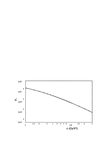
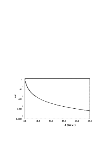
Figure 2: The fit of the form factors of the proton: (a) [left], the electromagnetic form factor $G(t)$ and and [right] the matter form factor $A(t)$. The circles are the moments of the GPDs (only every tenth point is shown).

4 Extension of the HEGS model with the spin-flip amplitude

In papers [67, 68], the new High Energy Generelized Structure model was developed. The central moment of the model is that it uses two form factors corresponding to charge and matter distributions calculated as the relevant moments of $GPDs(x,\xi=0,t)$. The basic Born spin-non-flip amplitudes were taken in the form

$$F_{h}^{Born}(s,t)\ =h_{1}\ G^{2}(t)\ F_{a}(s,t)\ (1+r_{1}/\hat{s}^{0.5})\ +h_{2}\ A^{2}(t)\ F_{b}(s,t)\ (1+r_{2}/\hat{s}^{0.5}),$$ (40)

where $F_{a}(s,t)$ and $F_{b}(s,t)$ have the standard Regge form

$$F_{a}(s,t)\ =\hat{s}^{\epsilon_{1}}\ e^{B(s)\ t},\ \ \ F_{b}(s,t)\ =\hat{s}^{\epsilon_{1}}\ e^{B(s)/4\ t}.$$ (41)

The slope of the scattering amplitude has the logarithmic dependence on energy, $B(s)=\alpha^{\prime}\ ln(\hat{s})$, with fixed $\alpha_{1}=0.24$ GeV^-2 and $\Delta=0.11$. Taking into account the Mandelstam region of the analyticity of the scattering amplitude for the $2\rightarrow 2$ scattering process with identical mass $s+u+t=4m_{p}^{2}$, one takes the normalized energy variable $s$ in a complex form $\hat{s}/s_{0}$ with $\hat{s}=se^{i\pi}$, and $s_{0}=4m_{p}^{2}$ where $m_{p}$ is the mass of the proton. In the present model, a small additional term is introduced into the slope, which reflects some possible small nonlinear properties of the intercept. As a result, the slope is taken in the form $B(s,t)\ =(\alpha_{1}+kqe^{-kq^{2}Ln(\hat{s}\ t)})Ln(\hat{s})$. This form leads to the standard form of the slope as $t\rightarrow 0$ and $t\rightarrow\infty$. Note that our additional term at large energies has a similar form as an additional term to the slope coming from the $\pi$ loop examined in Ref. [69] and recently in Ref. [70].

Then, as we intend to describe sufficiently low energies, possible Odderon contributions were taken into account:

$$F_{\rm odd}(s,t)\ =\pm\ h_{\rm odd}\ A^{2}(t)\ F_{b}(s,t),$$ (42)

where $h_{\rm odd}=ih_{3}t/(1-r_{0}^{2}t)$. Just as we supposed in the previous variant of the HEGS model that $F_{b}(s,t)$ corresponds to the cross-even part of the three-gluon exchange, our Odderon contribution is also connected with the matter form factor $A(t)$. Our ansatz for the Odderon slightly differs from the cross-even part by some kinematic function. The form of the Odderon working in all $t$ has the same behavior as the cross-even part at larger momentum transfer, of course, with different signs for proton-proton and proton-antiproton reactions.

The final elastic hadron scattering amplitude is obtained after unitarization of the Born term. So, first, we have to calculate the eikonal phase

$$\chi(s,b)\ =-\frac{1}{2\pi}\ \int\ d^{2}q\ e^{i\vec{b}\cdot\vec{q}}\ F^{\rm Born}_{h}\left(s,q^{2}\right)\,$$ (43)

and then obtain the final hadron scattering amplitude using eq.(9)

$$F_{h}(s,t)=is\ \int\ b\ J_{0}(bq)\ \Gamma(s,b)\ db\,\ \ \ {\rm with}\ \ \ \Gamma(s,b)=1-\exp[\chi(s,b)].$$ (44)

Note that the parameters of the model are energy independent. The energy dependence of the scattering amplitude is determined only by the single intercept and the logarithmic dependence on $s$ of the slope. The analysis of the hard Pomeron contribution in the framework of the model [72] shows that such a contribution is not felt. For the most part, the fitting procedure requires a negative additional hard Pomeron contribution. We repeat the analysis of [72] in the present model and obtain practically the same results. Hence, we do not include the hard Pomeron in the model.

Now we do not know exactly, also from a theoretical viewpoint, the dependence of different parts of the scattering amplitude on $s$ and $t$. So, usually, we suppose that the imaginary and real parts of the spin-nonflip amplitude behave exponentially with the same slope, whereas the imaginary and real parts of spin-flip amplitudes, without the kinematic factor $\sqrt{|t|}$, behave in the same manner with $t$ in the examined domain of transfer momenta. Moreover, one mostly assume the energy independence of the ratio of the spin-flip to spin-nonflip parts of the scattering amplitude. All this is our theoretical uncertainty.

Let us take the main part of the spin-flip amplitude in the basic form of the spin-non-flip amplitude. Hence, the born term of the spin-flip amplitude can be represented as

$$F_{sf}^{Born}(s,t)= h_{sf1}\ F_{1}^{2}(t)\ F_{sf-a}(s,t)\ (1+r_{sf1}/\hat{s}^{0.5})$$ (45)

$$+ h_{sf2}\ A^{2}(t)\ F_{sf-b}(s,t)\pm h_{sf-odd}\ A^{2}(t)F_{sf-b}(s,t)\ (1+r_{sf2}/\hat{s}),$$

where $F_{sf-a}(s,t)$ and $F_{sf-b}(s,t)$ are the same as in the spin-non-flip amplitude but, according to the paper [37], the slope of the amplitudes is essentially increasing. As a result, we take $F_{sf-a}(s,t)\ =\hat{s}^{\epsilon_{1}}\ e^{4B(s)\ t}$, and $F_{sf-b}(s,t)\ =\hat{s}^{\epsilon_{1}}\ e^{B(s)/2\ t}$. It is to be noted that most part of the available experimental data on the spin-correlation parameters exist only at sufficiently small energies. Hence, at lower energies we need to take into account the energy-dependent parts of the spin-flip amplitudes. In this case, some additional polarization data can be included in our examination. Then the spin-flip eikonal phase $\chi_{ls}(s,b)$ is calculated by the Fourier-Bessel transform, eq.(43), and then the spin-flip amplitude in the momentum transfer representation is obtained by the standard eikonal representation for the spin-flip part, eq.(12).

As in our previous works [73, 74], a small contribution from the energy-independent part of the spin-flip amplitude in a form similar to that proposed in Ref. [75] was added.

$$F_{sf-t}(s,t)\ =h_{sf}q^{3}F_{1}^{2}(t)e^{-B_{sf}q^{2}}.$$ (46)

It has two additional free parameters. We take into account $F_{sf-t}(s,t)$ and the full spin-flip amplitude is $F_{sf}(s,t)=F_{sf-ab}+F_{sf-t}$.

The model is very simple from the viewpoint of the number of fitting parameters and functions. There are no artificial functions or any cuts which bound the separate parts of the amplitude by some region of momentum transfer. We analyzed $3080$ experimental points in the energy region $9.8$ GeV $\leq\sqrt{s}\leq 8$ TeV and in the region of momentum transfer $0.000375\leq|t|\leq 10$ GeV² for the differential cross sections and $125$ experimental points for the polarization parameter $A_{N}$ in the energy region $4.5<\sqrt{s}<30$ GeV. The experimental data for the proton-proton and proton-antiproton elastic scattering are included in 87 separate sets of 30 experiments [76, 77], including the recent data from the TOTEM Collaboration at $\sqrt{s}=8$ TeV [78]. This gives us many experimental high-precision data points at a small momentum transfer, including the Coulomb-hadron interference region where the experimental errors are remarkably small. Hence, we can check our model construction where the real part is determined only by the complex representation of $\hat{s}=s/s_{0}exp(-i\pi/2)$. We do not include the data on the total cross sections $\sigma_{\rm tot}(s)$ and $\rho(s)$, as their values were obtained from the differential cross sections, especially in the Coulomb-hadron interference region. Including these data decreases $\chi^{2}$, but it would be a double counting in our opinion.

In the work, the fitting procedure uses the modern version of the program ”FUMILIM” [80, 81]” of the old program ”FUMILY” [82] which calculates the covariant matrix and gives the corresponding errors of the parameters and their correlation coefficients, and the errors of the final data. The analysis of the TOTEM data by three different statistical methods, including the calculations through the correlation matrix of the systematic errors, was made in [83].

As in the old version of the model, we take into account only the statistical errors in the standard fitting procedure. The systematic errors are taken into account by the additional normalization coefficient which is the same for every row of the experimental data. It essentially decreases the space of the possible form of the scattering amplitude. Of course, it is necessary to control the sizes of the normalization coefficients so that they do not introduce an additional energy dependence. Our analysis shows that the distribution of the coefficients has the correct statistical properties and does not lead to a visible additional energy dependence. As a result, we obtained a quantitative description of the experimental data ($\sum\chi^{2}/n_{dof}=1.3$).

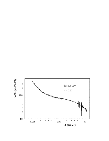
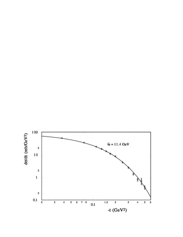
Figure 3: $d\sigma/dt$ for $pp$ [left] at $\sqrt{s}=9.8$ GeV and $p\bar{p}$ [right] at $\sqrt{s}=11.4$ GeV (lines - the model calculatios, points - the experimental data [79]).

In the model, a good description of the CNI region of momentum transfer is obtained in a very wide energy region (approximately 3 orders of magnitude) with the same slope of the scattering amplitude. The differential cross sections of the proton-proton and proton-antiproton elastic scattering at small momentum transfer are presented in Fig. 3 at $\sqrt{s}=9.8$ GeV for $pp$ scattering, and $\sqrt{s}=11$ GeV for $p\bar{p}$ elastic scattering. The model quantitatively reproduces the differential cross sections in the whole examined energy region in spite of the fact that the size of the slope is essentially changing in this region [due to the standard Regge behavior $log(\hat{s}$] and the real part of the scattering amplitude has different behavior for $pp$ and $p\bar{p}$.

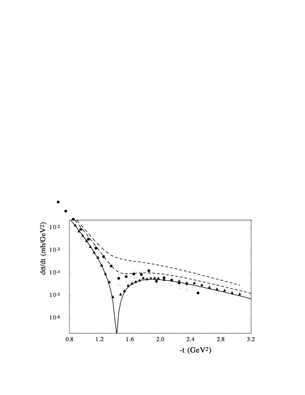
Figure 4: The model calculation of the diffraction minimum in $d\sigma/dt$ of $pp$ scattering at $\sqrt{s}=9.23,\ 13.76,\ 30.4$ GeV; lines - the model calculations (shirt dash, long dash and solid; circles and triangles - the experimental data at 13.4 and 30.7 GeV [79]).

The form and the energy dependence of the diffraction minimum are very sensitive to different parts of the scattering amplitude. The change of the sign of the imaginary part of the scattering amplitude determines the position of the minimum and its movement with changing energy. The real part of the scattering amplitude determines the size of the dip. Hence, it depends heavily on the odderon contribution. The spin-flip amplitude gives the contribution to the differential cross sections additively. So the measurement of the form and energy dependence of the diffraction minimum with high precision is an important task for future experiments. In Fig.4, the description of the diffraction minimum in our model is shown for $\sqrt{s}=9.23,\ 13.76$, and $\ 30.4\$GeV. The HEGS model reproduces sufficiently well the energy dependence and the form of the diffraction dip. In this energy region the diffraction minimum reaches the sharpest dip at $\sqrt{s}=30$ GeV. Note that at this energy the value of $\rho(s,t=0)$ also changes its sign in the proton-proton scattering. The $p\bar{p}$ cross sections in the model are obtained by the $s\rightarrow u$ crossing without changing the model parameters. And for the proton-antiproton scattering the same situation with correlations between the sizes of $\rho(s,t=0)$ and $\rho(s,t_{min})$ takes place at low energy (approximately at $p_{L}=100$ GeV). Note that it gives a good description for the proton-proton and proton-antiproton elastic scattering or $\sqrt{s}=53$ GeV and for $\sqrt{s}=62.1$ GeV. The diffraction minimum at $\sqrt{s}=7$ TeV and $\sqrt{s}=13$ TeV is reproduced sufficiently well too.

In the standard pictures, the spin-flip and double spin-flip amplitudes correspond to the spin-orbit $(LS)$ and spin-spin $(SS)$ coupling terms. The contribution to $A_{N}$ from the hadron double spin-flip amplitudes already at $p_{L}=6\$GeV/c is of the second order compared to the contribution from the spin-flip amplitude. So with the usual high energy approximation for the helicity amplitudes at small transfer momenta, we suppose that $\Phi_{1}=\Phi_{3}$ and we can neglect the contributions of the hadron parts of $\Phi_{2}-\Phi_{4}$. Note that if $\Phi_{1},\Phi_{3},\Phi_{5}$ have the same phases, their interference contribution to $A_{N}$ will be zero, though the size of the hadron spin-flip amplitude can be large. Hence, if this phase has different $s$ and $t$ dependences, the contribution from the hadron spin-flip amplitude to $A_{N}$ can be zero at $s_{i},\ t_{i}$ and non-zero at other $s_{j},\ t_{j}$.

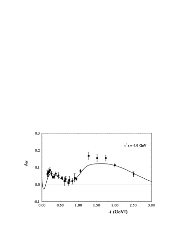
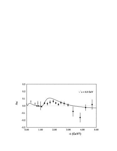
Figure 5: The analyzing power $A_{N}$ of pp - scattering calculated: a) at $\sqrt{s}=4.9\$GeV (the experimental data [84]), and b) at $\sqrt{s}=6.8\$GeV (points - the existing experimental data [85] ).

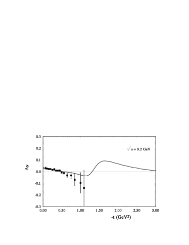
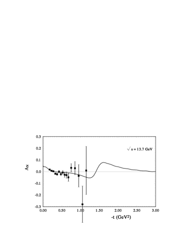
Figure 6: The analyzing power $A_{N}$ of pp - scattering calculated: a) at $\sqrt{s}=9.2\$GeV, (the experimental data [86]), and b) at $\sqrt{s}=13.7\$GeV (points - the experimental data [87]).

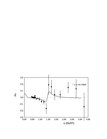
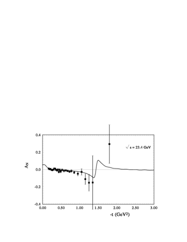
Figure 7: The analyzing power $A_{N}$ of pp - scattering calculated: a) at $\sqrt{s}=19.4\$GeV (the experimental data [88]), and b) at $\sqrt{s}=23.4\$GeV (points - the existing experimental data [87])

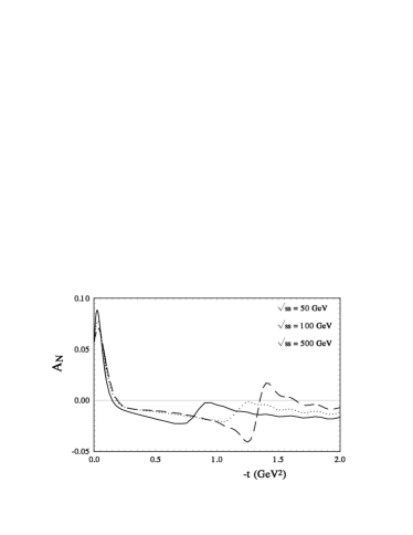
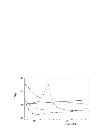
Figure 8: [left] The calculated size of the spin correlation parameter $A_{N}(s,t)$ at high energies $\sqrt{s}=50,\ 100,\ 500\$GeV. [right] the $s$-dependence of $A_{N}(s,t)$ at different fixed $t_{i}=0.001,\ 0.1,\ 0.4,1.0,1.5\$ GeV (solid, dots, short dash, dot-dot-dash and long-dash lines, respectively).

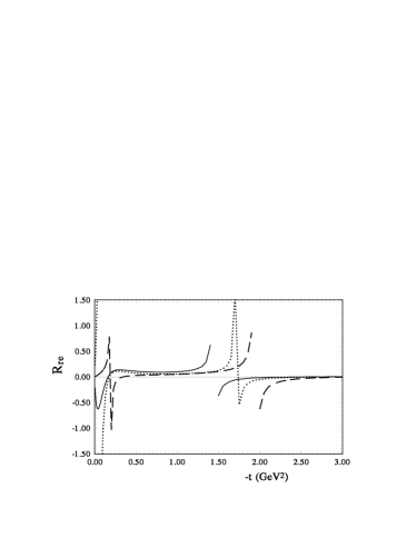
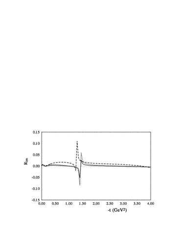
Figure 9: [left] The ratio of the imaginary parts of the spin-flip amplitude and spin-non-flip amplitude; [right] the ratio of the real parts of the spin-flip amplitude and spin-non-flip amplitudes (lines - dashed, dots, and solid correspond to $\sqrt{s}=9.23,\ 19.4,\ 30.7\$GeV).

Our calculation for $A_{N}(t)$ is shown in Fig. 5 a,b. at $\sqrt{s}=4.9$ GeV and $\sqrt{s}=6.8$ GeV. For our high energy model it is a very small energy. However, the description of the existing data is sufficiently good. At these energies, the diffraction minimum practically is overfull by the real part of the spin-non-flip amplitude and the contribution of the spin-flip-amplitude; however, the $t$-dependence of the analysing power is very well reproduced in this region of the momentum transfer. Note that the magnitude and the energy dependence of this parameter depend on the energy behavior of the zeros of the imaginary-part of the spin-flip amplitude and the real-part of the spin-nonflip amplitude. Figure 6 shows $A_{N}(t)$ at $\sqrt{s}=9.2$ GeV and $\sqrt{s}=13.7$ GeV. At these energies the diffraction minimum deepens and its form affects the form of $A_{N}(t)$. At last, $A_{N}(t)$ is shown at large energies $\sqrt{s}=19.4$ GeV and $\sqrt{s}=23.4$ GeV in Fig.7. The diffraction dip in the differential cross section has a sharp form and it affects the sharp form of $A_{N}(t)$. The maximum negative values of $A_{N}$ coincide closely with the diffraction minimum. We found that the contribution of the spin-flip to the differential cross sections is much less than the contribution of the spin-nonflip amplitude in the examined region of momentum transfers from these figures; $A_{N}$ is determined in the domain of the diffraction dip by the ratio

$$A_{N}\sim Imf_{-}/Ref_{+}.$$ (47)

The size of the analyzing power changes from $-45\%$ to $-50\%$ at $\sqrt{s}=50\ \,{\rm GeV}$ up to $-25\%$ at $\sqrt{s}=500\ \,{\rm GeV}$. These numbers give the magnitude of the ratio Eq.(47) that does not strongly depend on the phase between the spin-flip and spin-nonflip amplitudes. This picture implies that the diffraction minimum is mostly filled by the real-part of the spin-nonflip amplitude and that the imaginary-part of the spin-flip amplitude increases in this domain as well.

We observe that the dips are different in speed of displacements with energy from Fig. 4. In Fig. 8, one sees that at larger momentum transfers, $|t|\sim 2$ to $3\ \,{\rm(GeV}/c)^{2}$, the analyzing power depends on energy very weakly. The spin-flip amplitude gives the contribution to the differential cross sections additively. So the measurement of the form and energy dependence of the diffraction minimum with high precision is an important task for future experiments.

In Fig.8, the predictions of the HEGS model are presented for $A_{N}(t)$ up to high energies $\sqrt{s}=500$ GeV. It can be seen that at such huge energy the size of $A_{N}(t)$ does not come to zero and can be measured in new LHC experiments with a fixed target.

Now let us examine the ratio of the real and imaginary parts of the spin-flip phenomenological and model amplitudes to their imaginary parts of the hadron spin-non-flip amplitudes (see Figs. 9 (a,b) and 11 (a,b)). It is clear that this ratio can not be regarded as a constant. Moreover, this ratio has a very strong energy dependence.

Neglecting the $\Phi_{2}(s,t)-\Phi_{4}(s,t)$ contribution, the spin correlation parameter $A_{N}(s,t)$ can be written taking into account the phases of separate amplitudes

$$A_{N}(s,t)\frac{d\sigma}{dt}=-\frac{4\pi}{s^{2}}[|F_{nf}(s,t)|\ |F_{sf}(s,t)|Sin(\theta_{nf}(s,t)-\theta_{sf}(s,t))].$$ (48)

where $\theta_{nf}(s,t),\theta_{sf}(s,t)$ are the phases of the spin non-flip and spin-flip amplitudes. It is clearly seen that despite the large spin-flip amplitude the analyzing power can be near zero if the difference of the phases is zero in some region of momentum transfer. The experimental data at some point of the momentum transfer show the energy independence of the size of the spin correlation parameter $A_{N}(s,t)$. Hence, the small value of the $A_{N}(s,t)$ at some $t$ (for example, very small $t$) does not serve as a proof that it will be small in other regions of momentum transfer.

Let us compare the spin-flip amplitudes and the spin-nonflip amplitudes in the impact parameter representation at $\sqrt{s}=30$ GeV. The results are present in Fig.10. It can be seen that the first has more peripheral behavior.

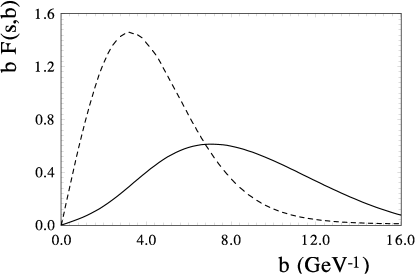
Figure 10: Impact parameter representation of the spin-nonflip and spin-flip amplitude at $\sqrt{s}=30$ GeV ($b(1-exp(-\chi_{nf}))$ - dashed line, and ($b(\chi_{sf}\ exp(-\chi_{nf}))$ - hard line)

5 Conclusions

The Generelized parton distributions (GPDs) make it possible to better understand the fine hadron structure and to obtain the hadron structure in the space frame (impact parameter representations). The important property of GPDs consists in that they are tightly connected with the hadron form factors. The new HEGS model gives a quantitative description of elastic nucleon scattering at high energy with a small number of fitting parameters. Our model of the GPDs leads to a good description of the proton and neutron electromagnetic form factors and their elastic scattering simultaneously. A successful description of the existing experimental data by the model shows that the elastic scattering is determined by the generalized structure of the hadron. It allows one to find some new features in the differential cross section of $pp$-scattering in the unique experimental data of the TOTEM collaboration at $\sqrt{s}=13$ TeV (small oscillations [89] and anomalous behavior at small momentum transfer [90] ). The inclusion of the spin-flip parts of the scattering amplitude allows one to describe the low energy experimental polarization data of the $pp$ elastic scattering. It is shown that the non-perturbative spin-effects at high energies may not be small.

It should be noted that the real part of the scattering amplitude, on which the form of the diffraction dip heavily depends, is determined in the framework of the HEGS model only by the complex $\bar{s}$, and hence it is tightly connected with the imaginary part of the scattering amplitude and satisfies the analyticity and the dispersion relations. The HEGS model reproduces well the form and the energy dependence of the diffraction dip of the proton-proton and proton antiproton elastic scattering [91].

The research into the form and energy dependence of the diffraction minimum of the differential cross sections of elastic hadron-hadron scattering at different energies will give valuable information on the structure of the hadron scattering amplitude and hence the hadron structure and the dynamics of strong interactions. The diffraction minimum is created under a strong impact of the unitarization procedure. Its dip depends on the contributions of the real part of the spin-non-flip amplitude and the whole contribution of the spin-flip scattering amplitude. In the framework of HEGS model, we show a deep connection between elastic and inealastic cross sections, which are tightly connected with the hadron structure at small and large distances.

Quantitatively, for different thin structures of the scattering amplitude, wider analysis is needed. This concerns the fixed intercept taken from the deep inelastic processes and the fixed Regge slope $\alpha^{\prime}$, as well as the form of the spin-flip amplitude. Such analysis requires a wider range of experimental data, including the polarization data of $A_{N}(s,t)$, $A_{NN}(s,t)$, $A_{LL}(s,t)$, $A_{SL}(s,t)$. The obtained information on the sizes and energy dependence of the spin-flip and double-flip amplitudes will make it possible to better understand the results of famous experiments carried out by A. Krish at the ZGS to obtain the spin-dependent differential cross sections [92, 93] and the spin correlation parameter $A_{NN}$, and at the AGS [94] to obtain the spin correlation parameter $A_{N}$ showing the significant spin effects at a large momentum transfer.

The present analysis, which includes the contributions of the spin-flip amplitudes, also shows a large contradiction between the extracted value of $\rho(s,t)$ and the predictions from the analysis based on the dispersion relations. However, our opinion is that additional analysis is needed, which will include additional corrections connected with the possible oscillation in the scattering amplitude and with the $t$-dependence of the spin-flip scattering amplitude. We hope that future experiments at NICA can give valuable information for the improvement of our theoretical understanding of strong hadron interaction.

References

- [1] S. V. Goloskokov, S. P. Kuleshov, O. V. Selyugin, ”Spin Spin effects in high energy hadron-hadron scattering”, Z. Phys. C 1991 50, 455-464.
- [2] M. Anselmino, S. Forte, ”Small angle polarization in high-energy p p scattering through nonperturbative chiral symmetry breaking”, Phys. Rev. Lett. 1993 71, 223-226.
- [3] N.F.Edneral, S.M.Troshin, N.E.Tyurin, ”On Spin Effects in Elastic Scattering at Large Momentum Transfers”. Pisma Zh.Eksp.Teor.Fiz. 1979 30, 356-360.
- [4] J. Soffer and T. T. Wu, ”A New Impact Picture for Low and High-Energy Proton Proton Elastic Scattering ”, Phys. Rev. D 1979 19, 3249–3256.
- [5] Yu.N. Uzikov and A.A. Temerbayev, ”Null-test signal for T-invariance violation in pd scattering”, Phys. Rev. C 2015 92, 014002-014009.
- [6] L.A. Koop, et all., ”Vozmojnosti izucheniya narusheniya chetnosti v stolknovenii yader na uskoritel’nom komplexse NICA”, Pis’ma v Zhurnal Fizika Elementarnykh Chastits i Atomnogo Yadra 2020 17, 122-131.
- [7] A.I. Milstein, N.N. Nikolaev, S.G. Salnikov, ”Parity Violation in Proton–Proton Scattering at High Energies”, Pis’ma v ZhETPF 2020 111, 215–219; [ JETP Letters, 2020 111, 197-201
- [8] L.I. Lapidus, ”The polarization effects in a interaction of hadrons at small momentum transfer”, Particles & Nuclei 1978 9, 84-96.
- [9] F. E. Low, ”A Model of the Bare Pomeron”, Phys. Rev. D 1875 12, 163–173; S. Nussinov, ”Colored Quark Version of Some Hadronic Puzzles”, Phys. Rev. Lett. 1975 34, 1286–1289.
- [10] P. V. Landshoff and O. Nachtmann, ”Vacuum Structure and Diffraction Scattering”, Z. Phys. C 1987 35, 405–408.
- [11] A. Donnachie and P. V. Landshoff, ”Gluon Condensate and Pomeron Structure”, Nucl. Phys. B 1989 311, 509–518.
- [12] L.L. Jenkovszky, ”Spin and Polarization in High-Energy Hadron-Hadron and Lepton-Hadron Scattering” arxiv: 2011.06432 [hep-ph] 2020.
- [13] K. Abe, Richard C. Fernow, T.A. Mulera, K.M. Terwilliger, W. de Boer et al. ”Measurement of Proton Proton Elastic Scattering in Pure Initial Spin States at 11.75-GeV/c ”, Phys.Lett.B 1976, em 63 239-244.
- [14] S. B. Nurushev, ”POLARIZATION STUDY”, Proc. of III Workshop on High Energy Spin Physics, Protvino, 1989, 5–37.
- [15] N. Akchurin, N. H. Buttimore and A. Penzo, ”Evaluation of the elastic p p single flip helicity amplitude at low momentum transfer and high-energies”, Phys. Rev. D 1995 51, 3944–3947.
- [16] O. V. Selyugin, ”What can be learnt from the new UA4/2 data”’ Phys. Lett. B 1994 333, 245-249.
- [17] M.Sawamoto, S.Wakaizumi, ”SPIN DEPENDENT FORCES IN ELASTIC P P SCATTERING AT 6-GEV/C ”, Proc Theor.Phis. 1979 62 (1979) 1293–1306.
- [18] Sibirtsev A., Haidenbauer J., Hammer H.W., Krewald S., Meißner U.G., ”Proton-proton scattering above 3 GeV/c”, Eur. Phys. J. A 2010 45 357–372.
- [19] C. Bourrely, J. Soffer, ”On the Size of the Coulomb-Nuclear Interference Polarization in Hadronic Reactions at High-Energy and Large Momentum Transfer”, Lett. Nuovo Cim. 1977 19, 569-572.
- [20] N. Bence, A. Lengyel, Z. Tarics, E. Martynov, G. Tersimonov, ”Froissaron and Maximal Odderon with spin-flip in pp and p¯p high energy elastic scattering”, arXiv:2010.11987 [hep-ph] 2020.
- [21] T. Chou and C. N. Yang, ”Hadronic Matter Current Distribution Inside a Polarized Nucleus and a Polarized Hadron”, Nucl. Phys. B 1976 107, 1-20.
- [22] A. E. Dorokhov, N. I. Kochelev and Yu. A. Zubov, ”Proton spin within nonperturbative QCD”, Int. Jour. Mod. Phys. A 1993 8, 603–651.
- [23] A. V. Efremov and O. V. Teryaev, ”On Spin Effects in Quantum Chromodynamics”, Sov.J.Nucl.Phys. 36 1982 36 140, Yad.Fiz. 36 1982 36 242-246.
- [24] R. Fiore, L. Jenkovszky, R. Orava, E. Predazzi, A. Prokudin, and O. Selyugin, ”Forward Physics at the LHC; Elastic Scattering”, Int.J.Mod.Phys. A 2009 24, 2551-2599.
- [25] Giulia Pancheri, Yogendra N. Srivastava ”Introduction to the physics of the total cross-section at LHC: A Review of Data and Models”, arXiv:1610.10038 [hep-ph]; Report number: MIT-CTP/4828, INFN-16-13/LNF, 2016, doi10.1140/epjc/s10052-016-4585-8
- [26] L. Frankfurt, C.E. Hyde, M. Strikman, C. Weiss, [hep-ph]/ 0719.2942 2007.
- [27] J. R. Cudell and O. V. Selyugin, ”Saturation and non-linear effects in diffractive processes”, Czech. J. Phys.(Syppl. A) 2004 54 A441–A445.
- [28] A.D. Krish, S.M. Troshin, ”Small P2Elastic Proton-Proton Polarization near 300 GeV”, hep-ph/9610537 1996.
- [29] Müller, D.; Robaschik, D.; Geyer, B.; Dittes, F.-M.; Hořejši, J. ”Wave Functions, Evolution Equations and Evolution Kernels from Light-Ray Operators of QCD”, Fortschr. Phys. 1994, 42, 101–105.
- [30] Ji, X. ”Deeply Virtual Compton Scattering”, Phys. Rev. 1997, D55, 7114–7118.
- [31] Radyushkin, A.V. ”Scaling Limit of Deeply Virtual Compton Scattering”, Phys. Lett. 1996, B380, 41–46.
- [32] Burkardt M., ”Generalized Parton Distributions for large x”, Phys.Lett. B 2004 595, 245–348. arXiv [ hep-ph/0401159].
- [33] Burkardt, M. ”Off-Forward Parton Distributions in 1+1 Dimensional QCD”, Phys. Rev. 2000, D62, 071503–071507.
- [34] Diehl, M. ”Generalized parton distributions in impact parameter space”, Eur. Phys. J. 2002, C25, 223–226.
- [35] N.F. Nelipa , Introduction to the theory of strong interaction elementary particles Moscow 1970.
- [36] M.L. Goldberger, and K.M. Watson, in book ”Collision Theory”, NY, 1964.
- [37] E. Predazzi and O.V. Selyugin, ”Behavior of the hadronic potential at Large Distances ” Eur.Phys.J. A 2002 13 471-475
- [38] E. Predazzi, ”DYNAMICAL MODEL FOR REGGE TRAJECTORIES”, 1969 PRINT-69-2891.
- [39] O.V. Selyugin, ”Is there exist a hadron spin-flip contribution in the Coulomb-hadron interference at small transfer momenta and high energies”, Eur.Phys.J.A 2006 28 83-89.
- [40] J.R. Cudell, E. Predazzi, O.V. Selyugin, ”Interactions at large distances and spin effects in nucleon-nucleon and nucleon-nuclei scattering”, Particles&Nuclei , 2004 35 S75–S78.
- [41] O. V. Selyugin, J. R. Cudell, ” Analytic properties of unitarization schemes”, Czech.J.Phys. 2006 56, F237–F243; arXiv:hep-ph/0611305, 2006.
- [42] O. V. Selyugin, J. -R. Cudell, E. Predazzi ”Analytic properties of different unitarization schemes”, Eur.Phys.J.ST2008, 162 37-42.
- [43] J. Bystricky and F. Lehar, C. Lechanoine-LeLuc and F. Lehar, ”Small-angle polarization in high-energy p-p scattering through”, Rev.Mod.Phys. 1993 65 47–79.
- [44] N. H. Buttimore, E. Gotsman, E. Leader, ”SPIN DEPENDENT PHENOMENA INDUCED BY ELECTROMAGNETIC HADRONIC INTERFERENCE AT HIGH-ENERGIES”, Phys. Rev. D 1987 35, 407–412.
- [45] S.B.Nurushev, A.P.Potylitsin, G.M.Radutsky, ”Elastic p p scattering for analyzing of proton polarization in Coulomb nuclear interference region”, Proc. V Workshop on HESP, Protvino 1993 321–325.
- [46] O.V. Selyugin, ” GPDs of the nucleons and elastic scattering at high energies”, Eur.Phys.J. C 2012 72, 2073–2076.
- [47] A.I. Akhiezer, I.Ya. Pomeranchuk, ” [Kogerentnoe rasseyanie gamma-lucheĭ yadrami] / Kohärente Streuung von gamma-Strahlen an Kernen”, Zh.Eksp.Teor.Fiz. 7 (1937) 5, 567-578, Phys.Z.Sowjetunion 11 (1937) 5, 478-497
- [48] H. Bethe, ”Scattering and polarization of protons by nuclei”, Ann. Phys. 1958 3, 190–240.
- [49] L.D. Soloviev, Zh.Eksp.Teor.Fiz., 1965, 49, 292-295.
- [50] J. Rix, R.M. Thaler, ” Separation of Strong and Electromagnetic Effects in Charged-Particle Scattering”, Phys. Rev., 1966 152, 1357–1364.
- [51] M.P. Locher, ”Relativistic treatment of structure in the Coulomb interference problem”, Nucl.Phys. B , 1967 2, 525–531.
- [52] G. B. West, D. R. Yennie, ”Coulomb interference in high-energy scattering”, Phis. Rev. 1968 172, 1413–1422.
- [53] M.M. Islam, ”Bethe’s Formula for Coulomb-Nuclear Interference”, Phys.Rev., 1967 162 1426–1428.
- [54] R. Cahn, ”Coulombic - Hadronic Interference in an Eikonal Model”, Zeitschr. fur Phys. C 1982 15, 253–259.
- [55] V.A. Petrov, ”Coulomb-Nuclear Interference:the Latest Modification”, Proceedings of the Steklov Institute of Mathematics, 2020 309 219-224.
- [56] O.V. Selyugin, ”Phase of the Coulomb amplitude in the second Born approximation”, Mod.Phys.Lett. A 1996 11, 2317–2323.
- [57] O.V. Selyugin, ” HADRON SPIN-FLIP AMPLITUDE AND SLOPE OF DIFFERENTIAL CROSS-SECTIONS”, Mod. Phys. Lett. A 1999, 14, 223–230.
- [58] O.V. Selyugin, ”Coulomb hadron phase factor and spin phenomena in a wide region of transfer momenta” , Phys.Rev. D 1999, 61, 074028 –074036.
- [59] R.G. Sachs, ”High-Energy Behavior of Nucleon Electromagnetic Form Factors”, Phys.Rev. 1962, 126, 2256–2260.
- [60] A.I. Akhiezer and M.P. Rekalo, Sov.J.Pat.Nucl. 1974, 3 41–45.
- [61] M.N. Rosenbluth, ”High Energy Elastic Scattering of Electrons on Protons”, Phys.Rev. 1950, 79, 615–619.
- [62] A.V. Radyushkin, ”Nonforward parton densities and soft mechanism for form-factors and wide angle Compton scattering in QCD”, Phys. Rev. D 1998 58 (1998) 114008–114011.
- [63] M. Guidal, M.V. Polyakov, A.V. Radyushkin, and M. Vanderhaeghen, ”Nucleon form-factors from generalized parton distributions”, Phys. Rev. D , 2005 72, 054013–054019.
- [64] O.V. Selyugin and O.V. Teryaev, ”Generalized Parton Distributions and Description of Electromagnetic and Graviton form factors of nucleon”, Phys.Rev. D 2009 79, 033003–033009.
- [65] O.V. Selyugin, ” Models of parton distributions and the description of form factors of nucleon”, Phys.Rev. D 2014 89, 093007–093012.
- [66] M. Diehl, T. Feldmann, R. Jakob and P. Kroll, ”Generalized parton distributions from nucleon form-factor data”, Eur.Phys.J. C, 2005 39 1–39.
- [67] O.V. Selyugin, ” GPDs of the nucleons and elastic scattering at high energies ”, Eur.Phys.J. C 2012, 72, 2073–2076.
- [68] O.V. Selyugin, ”Nucleon structure and the high energy interactions”, Phys. Rev. D, 2015 91, 11303–11308.
- [69] A. Anselm and V. Gribov, ”Zero pion mass limit in interactions at very high-energies”, Phys. Lett. B 1972, 40, 487–493.
- [70] V. Khoze, A. D. Martin, M. G. Ryskin, ”Elastic proton-proton scattering at 13 TeV”, Phys. Rev. D 97, 034019 (2018).
- [71] V.A. Khoze, A.D. Martin and M.G. Ryskin, ”t dependence of the slope of the high energy elastic pp cross section ”, J.Phys.G 42 2015 42 025003.
- [72] O. V. Selyugin, ”Hard and soft pomerons in the elastic nucleon scattering”, Nucl.Phys. A , 2013, 903, 54-64.
- [73] O. V. Selyugin, ”High Energy Hadron Spin Flip Amplitude”, Particles and Nuclei Letters, 2016, 13, 303–309.
- [74] O. V. Selyugin ”Hadron structure and spin effects in elastic hadron scattering at NICA energies”, arXiv:2010.14767 [hep-ph], 2020.
- [75] M.V. Galynskii, E.A. Kuraev, ”Alternative way to understand the unexpected results of the JLab polarization experiments to measure the Sachs form factors ratio”, Phys.Rev. D 2014, 89, 054005 –054010.
- [76] Whalley, M.R., ”The HEPDATA database: The DURHAM-RAL database project”, in ”Workshop on Detector and Event Simulation in High-energy Physics (MC ’91)”, 1991 139.
- [77] K.R. Schubert, ”Elastic and Inelastic Hadron Diffraction at High-Energies”, In Landolt-Bronstein, New Series, 1979, 1/9a.
- [78] The TOTEM Collaboration (G. Antchev et al.), ” Evidence for non-exponential elastic proton–proton differential cross-section at low and TeV by TOTEM”, Nucl. Phys. B, 2015 899, 527-546.
- [79] Whalley, M.R., ”The HEPDATA database: The DURHAM-RAL database project”, Workshop on Detector and Event Simulation in High-energy Physics (MC ’91), (1991) 139.
- [80] I.M. Sitnik, ”Development of the FUMILI minimization package”, Comp.Phys.Comm. , 2014, 185 599–603.
- [81] I.M. Sitnik, I.I. Alexeev, O.V. Selyugin, ”The final version of the FUMILIM minimization package”, Comp.Phys.Comm., 2020, 251 107202–107207.
- [82] I.N. Silin, ”FUMILI”, CERN Program Library , 1983 D510.
- [83] J. R. Cudell, O. V. Selyugin, ” TOTEM data and the real part of the hadron elastic amplitude at 13 TeV”, arXiv:1901.05863 , hep-ph, 2019.
- [84] S.L. Kramer et al., ”Polarization Parameter for Nucleon-Nucleon Elastic Scattering at 11.8-GeV/c ”, Phys.Rev. D 1978, 17, 1709–1718.
- [85] J.Antille et al., ” MEASUREMENT OF THE POLARIZATION PARAMETER IN 24-GeV/c P P ELASTIC SCATTERING AT LARGE MOMENTUM TRANSFERS” 1981 Nuclear Physics B, 1981, 185, 1-19.
- [86] A.Gaudot et al., ”Polarization Measurements in pi+ p, K+ p and p p Elastic Scattering at 45-GeV/c and Comparison with Regge Phenomenology”, Phys.Lett. B 1976, 61, 103-110.
- [87] R.V.Kline et al., ”POLARIZATION PARAMETERS AND ANGULAR DISTRIBUTIONS IN PI+- P ELASTIC SCATTERING AT 100-GEV/C AND IN P P ELASTIC SPhys.Lett. B 1981, 105, 309–316.
- [88] G. Fidegaro et al., ”MEASUREMENT OF THE DIFFERENTIAL CROSS-SECTION AND OF THE POLARIZATION PARAMETER IN p p ELASTIC SCATTERING AT 200-GeV/c”, Phys.Lett. B, ???, 105, 309–316.
- [89] O. V. Selyugin, ”New feature in the differential cross sections at 13 TeV be measured at the LHC”, Phy.Lett. B , 2019, 797, 134870–134873.
- [90] O. V. Selyugin, ”Anomaly in the differential cross sections at 13 TeV”, arXiv:2009.10129 [hep-ph hep-ex], 2020.
- [91] O. V. Selyugin, ”The energy dependence of the diffraction minimum in the elastic scattering and new LHC data”, Nucl.Phys. A, 2017, 959, 116-128.
- [92] O’Fallon (Argonne) et al., ”High p-Transverse**2 Elastic p p Scattering”, Phys. Rev. D, 2014, 89, 093007–0930012.
- [93] G.R. Court, D.G. Crabb, I. Gialas, F.Z. Khiari, A.D. Krisch et al. ” Energy Dependence of Spin Effects in pp (Polarized) to pp (Polarized)” Phys.Rev.Lett. 1986 em 57 507–510.
- [94] D.G. Crabb (Michigan U.) et al., ”High precision measurement of A in large P(T)**2 spin polarized 24-GeV/c proton proton elastic scattering”, Phys.Rev.Lett., 1990, 65, 3241–3244. :