SpaceGroupIrep: A package for irreducible representations of space group

Abstract

We have developed a Mathematica program package SpaceGroupIrep which is a database and tool set for irreducible representations (IRs) of space group in BC convention, i.e. the convention used in the famous book “The mathematical theory of symmetry in solids” by C. J. Bradley & A. P. Cracknell. Using this package, elements of any space group, little group, Herring little group, or central extension of little co-group can be easily obtained. This package can give not only little-group (LG) IRs for any k-point but also space-group (SG) IRs for any k-stars in intuitive table form, and both single-valued and double-valued IRs are supported. This package can calculate the decomposition of the direct product of SG IRs for any two k-stars. This package can determine the LG IRs of Bloch states in energy bands in BC convention and this works for any input primitive cell thanks to its ability to convert any input cell to a cell in BC convention. This package can also provide the correspondence of k-points and LG IR labels between BCS (Bilbao Crystallographic Server) and BC conventions. In a word, the package SpaceGroupIrep is very useful for both study and research, e.g. for analyzing band topology or determining selection rules.

Program summary

Program title: SpaceGroupIrep

Developer’s respository link: https://github.com/goodluck1982/SpaceGroupIrep

Licensing provisions: GNU General Public Licence 3.0

Distribution format: tar.gz

Programming language: Mathematica

Classification: 11.2

External routines/libraries used: spglib (http://spglib.github.io/spglib)

Nature of problem: Space groups and their representations are important mathematical language to describe symmetry in crystals. The book—“The mathematical theory of symmetry in solids” by C. J. Bradley & A. P. Cracknell (called the BC book)—is highly influential because it contains not only systematic theory but also detailed complete data of space groups and their representations. The package SpaceGroupIrep digitizes these data in the BC book and provides tens of functions to manipulate them, such as obtaining group elements and calculating their multiplications, identifying k-points, showing the character table of any little group, determining the little-group (LG) irreducible representations (IRs) of energy bands, and calculating the direct product of space-group (SG) IRs. This package is a useful database and tool set for space groups and their representations in BC convention.

Solution method: The direct data in the BC book is used to calculate the LG IRs for standard k-points defined in the book. For a non-standard k-point, we first relate it to a standard k-point by an element which makes the space group self-conjugate and then calculate the LG IRs through the element. SG IRs are obtained by calculating the induced representations of the corresponding LG IRs. The full-group method based on double coset is used to calculate the direct products of SG IRs. In addition, an external package spglib is utilized to help convert any input cell to a cell in BC convention.

1 Introduction

Symmetry embodies the beauty of natural law and hence plays an important role in physics. A famous example is the Noether’s theorem which relates symmetric invariance to conserved quantities. Another example is various selection rules determined by symmetry. Furthermore, in recent years point-group (PG) and space-group (SG) symmetries demonstrate deep connections to topological physics such as topological insulators[1], topological crystalline insulators[2, 3], Dirac and Weyl semimetals[4, 5], nodal line and nodal loop semimetals[6, 7, 8], nodal chain metals[9], hourglass-band materials [10, 11, 12], topological photonic crystals with all-dielectric materials[13, 14, 15, 16]. In addition, representation theory of space group is also used in symmetry indicator method or elementary band representation method to classify symmetry-protected band topology of nonmagnetic materials[17, 18, 19, 20, 21, 22, 23, 24, 25, 26, 27], which greatly helps to search materials with specific band topology systematically.

Although nearly all modern codes of density functional theory (DFT) support symmetry analysis such as doing the Brillouin zone (BZ) integration in a symmetrically irreducible wedge region of BZ to accelerate calculation, none of them gives full information of space groups and their representations as far as we know. DFT codes VASP[28] and ABINIT[29] gives SG operations in their output files and ABINIT also provides the SG name, but neither of them give the information about the little-group (LG) irreducible representations (IRs). It’s known that SG IR is obtained by inducing from LG IR (also called small representation), and in most cases LG IR is enough for symmetry analysis. DFT codes WIEN2k[30] and Quantum ESPRESSO[31] can give LG IRs in the simple case of symmorphic space groups, but neither of them can process LG IRs with wave vectors (i.e. k-points) on the boundary of BZ for nonsymmorphic space groups. The manual of WIEN2k says “It will not work in cases of non-symmorphic spacegroups AND k-points at the surface of the BZ” for its program IRREP, while in the output of band.x of Quantum ESPRESSO there are remarks “zone border point and non-symmorphic group, symmetry decomposition not available”.

In order to determine the LG IRs of Bloch states there are mainly two steps: the first step is to calculate the characters of each operation in the little group, and the second step is to identify the LG IRs by looking up the character tables of LG IRs. In fact, the character tables of LG IRs were given by several books decades ago[32, 33, 34, 35, 36]. Then why few DFT codes can give LG IRs in all cases? We think the main reason is that the large amount of data relating to all LG IRs and the not-so-easy relations among the data to those who are not very familiar with the representation theory of space groups hinder the realization of full support of LG IRs in the DFT codes. On the contrary, in the simple case of symmorphic space groups which can be treated by WIEN2k and Quantum ESPRESSO, only PG character tables are needed to determine LG IRs, and PG character tables have much smaller data amount of several pages compared to those of LG IRs which can fill a book of hundreds of pages.

In fact, there have been third-party databases of SG/LG IRs available for a long time, i.e. the ISOTROPY software suite[37, 38] and the Bilbao Crystallographic Server (BCS)[39, 40]. The ISOTROPY is a collection of programs using space group theory to analyze phase transitions in crystals. It contains and provides all the data of SG IRs, but it does not give the data of LG IRs directly. And it does not have IR data of double space groups either, because they are not needed to analyze phase transitions in crystals. On the other hand, the BCS is a user-friendly website with various crystallographic databases and programs available online. It has full support of LG IRs and SG IRs for both space groups and double space groups. However, all the IR data are online and BCS does not provide offline programs. For common users, this makes BCS not convenient for batch processing a large number of offline jobs. Only recently, has there been a program called irvsp capable of calculating the LG IRs of Bloch states[41]. The irvsp is a post-processing program written in fortran and designed to calculate the LG IRs of Bloch states generated by VASP according to the character tables of LG IRs of BCS (obtained from a developer of BCS).

Historically, there are different conventions used to describe space groups and their IRs by different authors, such as Kovalev convention[32], Zak-Casher-Glück-Gur (ZCGG) convention[34], Bradley-Cracknell (BC) covention[35], and Cracknell-Davies-Miller-Love (CDML) convention[36]. Both ISOTROPY and BCS use the CDML convention. However, after we analyzed the times cited of these conventions on Web of Science[42] , we found that the BC convention is the most used one, especially in recent years, as shown in Fig. 1. This is not surprising, because the BC book not only contains the tables of LG IRs and related complete data but also contains comprehensive and systematic theory of space group and its representation, which makes it a classic reference book and teaching material. In addition, the BC book [35] is on sale and hence the most easily obtained one while the other books [32, 34, 36] are all out of print and hardly obtained. For example, we have tried our best to seek the CDML book [36] and failed finally, and hence we can only understand the CDML convention from ISOTROPY or BCS indirectly. The first version of the BC book was published in 1972 and a reprint version was published in 2009. We think, it was the popularity of the BC book that led to its reprint in 2009, and the reprint made the BC book easily obtained and more popular.

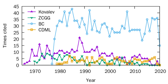
Figure 1: Times cited of the books [32], [34], [35], and [36] in each year on Web of Science, corresponding to the Kovalev, ZCGG, BC, and CDML conventions of space groups and their IRs respectively. The data are up to Aug. 2020.

Although the BC book is popular, the space group settings used in it are different from the commonly used settings in “International Tables for Crystallography, Volume A” (hereafter referred to as ITA)[43]. This maybe make the BC settings of space groups not very intuitive. Additionally, there are various tables correlated with each other in the BC book, which makes it somewhat tedious and complicated to extract information from these tables. For example, if we want to know the character of the operation $\{\sigma_{z}|\frac{1}{4}\frac{1}{4}\frac{1}{4}\}$ in the IR $\Gamma_{2}^{+}$ of space group $Fddd$ (No. 70) we have to first look up the Tab. 5.7 in the BC book (hereafter referred to as “BC-Tab. 5.7”) to find the abstract group $G_{8}^{3}$, the generators of the Herring little group (HLG) $\{C_{2z}|000\}$, $\{C_{2y}|000\}$, $\{I|\frac{1}{4}\frac{1}{4}\frac{1}{4}\}$, and the letter “b” according to which we can know that the IR $\Gamma_{2}^{+}$ is the IR $R_{2}$ of $G_{8}^{3}$ from BC-Tab. 5.8. Then we calculate the elements of HLG according to the generators $P=\{C_{2z}|000\}$, $Q=\{C_{2y}|000\}$, $R=\{I|\frac{1}{4}\frac{1}{4}\frac{1}{4}\}$ of $G_{8}^{3}$ in BC-Tab. 5.1 and find that $C_{6}=PR=\{\sigma_{z}|\frac{1}{4}\frac{1}{4}\bar{\frac{3}{4}}\}$. Hence we find in the character table of BC-Tab. 5.1 that the character of $\{\sigma_{z}|\frac{1}{4}\frac{1}{4}\bar{\frac{3}{4}}\}$ in IR $R_{2}$ of $G_{8}^{3}$ is $-1$. According to the properties of LG IR [refer to Eq. (2)] we know that the character of $\{\sigma_{z}|\frac{1}{4}\frac{1}{4}\frac{1}{4}\}$ in IR $\Gamma_{2}^{+}$ is $\chi(\{\sigma_{z}|\frac{1}{4}\frac{1}{4}\frac{1}{4}\})=e^{-i\bm{k}\cdot\Delta\bm{R}}\chi(\{\sigma_{z}|\frac{1}{4}\frac{1}{4}\bar{\frac{3}{4}}\})=\chi(\{\sigma_{z}|\frac{1}{4}\frac{1}{4}\bar{\frac{3}{4}}\})=-1$, in which $\bm{k}$ is $\Gamma$ and $\Delta\bm{R}=(\frac{1}{4}\frac{1}{4}\frac{1}{4})-(\frac{1}{4}\frac{1}{4}\bar{\frac{3}{4}})=(001)$. Furthermore, the rotation matrices used to calculate the HLG are defined in BC-Tab. 3.2. This example shows the cumbersome process of extracting information from the tables of the BC book. If lots of data are obtained this way manually, it’s not only tedious but also prone to error. Consequently, a program based on the SG and IR data in the BC book and capable of automating this process is highly required. However, there are no such programs available as we know, therefore we developed such a program package named SpaceGroupIrep in the Mathematica language.

Different conventions use different notations to label the LG IRs, therefore the meanings of IR labels are clear only if the convention used is pointed out. It is particularly true for the ZCGG, BC, and CDML conventions, because they use similar labels such as $\Gamma_{1},\Gamma_{2},\cdots,X_{1},X_{2},\cdots$ (called “$\Gamma$ labels” here) but with probably different meanings. A concomitant problem is how to find the correspondence between the IR labels of two different conventions. The only route we know before our SpaceGroupIrep is to use ISOTROPY. ISOTROPY can give the correspondence of IR labels for all the Kovalev, ZCGG, BC, and CDML conventions. However, ISOTROPY works only for high-symmetry (HS) k-points but not for HS lines, and ISOTROPY does not distinguish a couple of complex conjugate IRs related by time reversal symmetry. Furthermore, ISOTROPY does not support IRs of double space groups. Based on these reasons, at present we have realized the correspondence of LG IR labels between BC convention and CDML convention in SpaceGroupIrep. Notice that hereafter the CDML convention will be called BCS convention, because the CDML IR data we used are actually the BCS IR data collected from the output of irvsp.

The SpaceGroupIrep package contains all necessary data related to space groups and their IRs defined in the BC book and tens of functions manipulating the data. It can give both the LG IRs and SG IRs at any k-point in an intuitive table form. It can calculate the reduction of the direct product of two SG IRs. It can read the trace.txt file generated by vasp2trace[27] and determine the LG IRs in BC convention for all Bloch states. It can give the correspondence of LG IR labels between BC convention and BCS convention. It can also convert any given crystalline structure to the one in BC convention with the help of an external package spglib[44]. The above aspects are also true for double-valued IRs. In addition, SpaceGroupIrep can help study and understand the BC book. It can easily give the elements of a designated space group, little group, Herring little group, or central extension of little co-group and calculate the multiplication of the elements. In a word, the SpaceGroupIrep package is a database and tool set for SG/LG IRs in BC convention, which is very useful in both study and research.

2 Theory

2.1 Representation theory overview

Let $G$ be a space group whose elements are in the form of Seitz symbol $\{R|\bm{v}\}$. $\{R|\bm{v}\}$ means a rotation $R$ followed by a translation by vector $\bm{v}$. Select one k-point from each wave vector star (i.e. k-star) arbitrarily. Then the induced representations of all the allowed LG IRs of these selected k-points are just all the SG IRs of $G$. Let $\bm{k}$ be a wave vector, its little group be $G^{\bm{k}}$, and its wave vector star be ${}^{*}\bm{k}$. Suppose that $\Gamma_{p}^{\bm{k}}$ is the $p$-th allowed LG IR of $G^{\bm{k}}$ with dimension $d_{p}$. The modifier “allowed” means that $\Gamma_{p}^{\bm{k}}$ satisfies

$$\Gamma_{p}^{\bm{k}}(\{E|\bm{t}\})=e^{-i\bm{k}\cdot\bm{t}}\Gamma_{p}^{\bm{k}}(\{E|\bm{0}\})=e^{-i\bm{k}\cdot\bm{t}}I_{p},$$ (1)

where $E$ is the identity element of point group, $\bm{t}$ is a lattice vector, hence $\{E|\bm{t}\}$ is a pure translation operation, and $I_{p}$ is a $d_{p}\times d_{p}$ identity matrix. This allowing condition makes LG IRs compatible with the IRs of translation group $T$, and it also makes the representation matrices of all LG elements with the same rotation easily obtained through the relation

$$\Gamma_{p}^{\bm{k}}(\{R|\bm{v}+\bm{t}\})=e^{-i\bm{k}\cdot\bm{t}}\Gamma_{p}^{\bm{k}}(\{R|\bm{v}\})$$ (2)

if $\Gamma_{p}^{\bm{k}}(\{R|\bm{v}\})$ is known. If not explicitly stated otherwise, all the LG IRs we mentioned are allowed. Use $\{R_{\alpha}|\bm{\tau}_{\alpha}\}$ $(\alpha=1,2,\cdots,m_{\bm{k}})$ to denote the coset representatives of the left cosets of $G^{\bm{k}}$ in $G$. Then the SG IR induced from $\Gamma_{p}^{\bm{k}}$, denoted by $\Gamma_{p}^{\bm{k}}\uparrow G$ or ${}^{*}\Gamma_{p}^{\bm{k}}$ , is an $m_{\bm{k}}d_{p}$-dimensional IR and is determined by

$$\big{[}{}^{*}\Gamma_{p}^{\bm{k}}(\{R|\bm{v}\})\big{]}_{\alpha\beta}=\begin{cases}\Gamma_{p}^{\bm{k}}(\{R_{\alpha}|\bm{\tau}_{\alpha}\}^{-1}\{R|\bm{v}\}\{R_{\beta}|\bm{\tau}_{\beta}\})&\ \ \text{if }\{R_{\alpha}|\bm{\tau}_{\alpha}\}^{-1}\{R|\bm{v}\}\{R_{\beta}|\bm{\tau}_{\beta}\}\in G^{\bm{k}}\\ 0&\ \ \text{otherwise}\end{cases},$$ (3)

where $m_{\bm{k}}=|G|/|G^{\bm{k}}|$ is the number of k-points in the star ${}^{*}\bm{k}$, and $|G|$ means the order of the group $G$. It can be seen that LG IRs have to be known first to determine SG IRs. Consequently, the core problem in SG representation theory is to obtain all LG IRs of a space group.

The projective representation method is a general method to obtain LG IRs. Suppose $\{R_{i}|\bm{v}_{i}\}$ is one of the coset representatives of the cosets of $T$ in $G^{\bm{k}}$, and then the set of $R_{i}$ is the little co-group of $G^{\bm{k}}$, denoted by $\bar{G}^{\bm{k}}.$ Further suppose that $\tilde{D}_{p}^{\bm{k}}$ is the $p$-th projective representation of $\bar{G}^{\bm{k}}$ with factor system $\mu(R_{i},R_{j})=\exp[-i(R_{i}^{-1}\bm{k}-\bm{k})\cdot\bm{v}_{j}]$, then the LG IR $\Gamma_{p}^{\bm{k}}$ is determined by the following simple relation

$$\Gamma_{p}^{\bm{k}}(\{R|\bm{v}\})=e^{-i\bm{k}\cdot\bm{v}}\tilde{D}_{p}^{\bm{k}}(R).$$ (4)

To obtain the projective representation $\tilde{D}_{p}^{\bm{k}}$ of the little co-group $\bar{G}^{\bm{k}}$, we can resort to the central extension of $\bar{G}^{\bm{k}}$, denoted by $\bar{G}^{\bm{k}*}$. The group elements of $\bar{G}^{\bm{k}*}$ are in the form of $(R_{i},\alpha)$ with $\alpha=0,1,\cdots,g-1$ and $g$ is the smallest positive integer determined by the factor system

$$\mu(R_{i},R_{j})=\exp[-i(R_{i}^{-1}\bm{k}-\bm{k})\cdot\bm{v}_{j}]=\exp[2\pi ia(R_{i},R_{j})/g]$$ (5)

for all $i,j,$ in which the function $a(R_{i},R_{j})$ determined by $\mu(R_{i},R_{j})$ has integer value also in range $[0,g-1]$. The group multiplication of central extension $\bar{G}^{\bm{k}*}$ is defined as

$$(R_{i},\alpha)(R_{j},\beta)=(R_{i}R_{j},\;\alpha+\beta+a(R_{i},R_{j})\!\!\mod\,g)$$ (6)

with the property

$$(R_{i},\alpha)=(R_{i},0)(E,\alpha)=(E,\alpha)(R_{i},0).$$ (7)

Then all the irreducible projective representations we need can be obtained from the allowed ordinary IRs of the corresponding central extension. Suppose $\Delta_{p}^{\bm{k}}$ is the $p$-th allowd IR of $\bar{G}^{\bm{k}*}$ with the property

$$\Delta_{p}^{\bm{k}}((E,\alpha))=e^{i2\pi\alpha/g}I_{p},$$ (8)

and then the irreducible projective representation $\tilde{D}_{p}^{\bm{k}}$ is determined by

$$\tilde{D}_{p}^{\bm{k}}(R_{i})=\Delta_{p}^{\bm{k}}((R_{i},0)).$$ (9)

Apart from the projective representation method which is available for any k-point, there is a Herring little group method which is easier but only available for HS k-points. The HLG of $\bm{k},$ denoted by $\vphantom{G^{\bm{k}}}{}^{H}\!G^{\bm{k}}$, is a quotient group defined by $\vphantom{G^{\bm{k}}=G^{\bm{k}}/T^{\bm{k}}}{}^{H}\!G^{\bm{k}}=G^{\bm{k}}/T^{\bm{k}}$ in which $T^{\bm{k}}$ is a subgroup of $T$ with all translations $\{E|\bm{t}\}$ satisfying $e^{-i\bm{k}\cdot\bm{t}}$=1. When $\bm{k}$ is a HS k-point , $T^{\bm{k}}$ is an infinite group and hence $\vphantom{G^{\bm{k}}}{}^{H}\!G^{\bm{k}}$ is a finite group whose order is not very large. Then the IRs of $G^{\bm{k}}$ can be obtained directly from the IRs of $\vphantom{G^{\bm{k}}}{}^{H}\!G^{\bm{k}}$. Suppose $\vphantom{D_{p}^{\bm{k}}}{}^{H}\!D_{p}^{\bm{k}}$ is the $p$-th IR of $\vphantom{G^{\bm{k}}}{}^{H}\!G^{\bm{k}}$ and then the LG IR $\Gamma_{p}^{\bm{k}}$ of $G^{\bm{k}}$ is determined by

$$\Gamma_{p}^{\bm{k}}(\{R_{i}|\bm{v}_{i}\})=\vphantom{D_{p}^{\bm{k}}(}^{H}\!D_{p}^{\bm{k}}(\{R_{i}|\bm{v}_{i}\}T^{\bm{k}}).$$ (10)

When $\bm{k}$ is not a HS k-point, $\vphantom{G^{\bm{k}}}{}^{H}\!G^{\bm{k}}$ is generally an infinite group whose IRs are not easily obtained. In this case the HLG method loses its advantage over the projective representation method. Accordingly, the BC book uses both the two methods to describe the LG IRs in BC-Tabs. 5.7 and 6.13, i.e., it uses HLG to describe HS k-points and uses central extension of little co-group to describe k-points on HS lines. And each HLG or central extension is isomorphic to a certain abstract group $G_{m}^{n}$ whose IRs are known and given in BC-Tab. 5.1.

2.2 Brillouin zone and k-points

Generally, the Wigner-Seitz unit cell in reciprocal space is used as the (first) BZ. But for triclinic and monotonic Bravais lattices, their Wigner-Seitz BZs are dependent very much on the actual values of the lattice parameters and are difficult to draw or visualize. Therefore, in practice, the BC book uses the reciprocal primitive cell, i.e. a parallelepiped centered at $\bm{k}=0$, as the BZ for triclinic and monotonic Bravais lattices (and so does BCS). For other Bravais lattices, Wigner-Seitz BZs are used in the BC book. In spite of defining BZ this way, the shape of BZ is not always unique to each Bravais lattice. Depending on the ratios of lattice constants, there are more than one type (or shape) of BZ for base-centered orthorhombic [(a), (b) two types], body-centered orthorhombic [(a), (b), (c) three types], face-centered orthorhombic [(a), (b), (c), (d) four types], body-centered tetragonal [(a), (b) two types, see Fig. 2], and trigonal [(a), (b) two types] Bravais lattices. These five kinds of Bravais lattices are called “multiple-BZ Bravais lattices”. There are in total 22 different types of BZs for the 14 Bravais lattices which are shown in BC-Figs. 3.2 to 3.15.

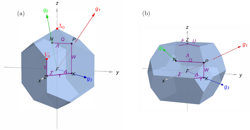
Figure 2: Two different types of BZs for body-centered tetragonal Bravais lattice with lattice constants $a$ and $c$: (a) for $a>c$ and (b) for $a<c$. Black capital letters are HS k-points, and purple ones are HS lines. Except the two auxiliary points $\Lambda_{0}$ and $V_{0}$, the two BZs are generated by showBZDemo["TetrBody(a)"] and showBZDemo["TetrBody(b)"] respectively.

HS k-points and k-points on HS lines in the basic domain are defined in BC-Tab. 3.6, and all the k-points in BC-Tab. 3.6 are termed “BC standard k-points” here. For multiple-BZ Bravais lattices, one k-point name may have different coordinates for different BZ types, but these coordinates are equivalent (differing by a reciprocal lattice vector) to each other with only one exception which is the $F$ k-point of trigonal lattice with coordinates $(0\frac{1}{2}\bar{\frac{1}{2}})$ and $(\frac{1}{2}\frac{1}{2}0)$ for BZ types (a) and (b) respectively. This means that for a space group the LG IRs for a given k-point name do not depend on BZ types, except for $F$ k-point in space groups of trigonal lattice. This is demonstrated as the two entries “(a) $F$” and “(b) $F$” existing in BC-Tabs. 5.7 and 6.13 for space groups of trigonal lattice.

Also for a multiple-BZ Bravais lattice, k-points on some HS lines are named only for certain BZ types but not for others. Take body-centered tetragonal lattice for example, $V$ HS line only exists in (a) type BZ, while $F$ and $U$ HS lines only exist in (b) type BZ, as shown in Fig. 2. In fact, both $\Lambda$ and $V$ in Fig. 2(a) correspond to the $\Lambda$ in Fig. 2(b). This can be analyzed as follow. The $\Lambda$ HS lines in both (a) and (b) type BZs have coordinates $(uu\bar{u})$ (here we use $u$ for the $\alpha$ in BC-Tab. 3.6), but the range of $u$ is different. The $\Lambda$ in (b) type BZ is from $\Gamma$ $(000)$ to $Z$ $(\frac{1}{2}\frac{1}{2}\bar{\frac{1}{2}})$ with $u\in(0,\frac{1}{2})$, while the $\Lambda$ in (a) type BZ is from $\Gamma$ $(000)$ to $\Lambda_{0}$ $(\lambda_{0}\lambda_{0}\bar{\lambda}_{0})$ with $u\in(0,\lambda_{0}]$ and $\lambda_{0}=\frac{1}{4}+\frac{c^{2}}{4a^{2}}<\frac{1}{2}$ ($a$ and $c$ are lattice constants and $a>c$ for (a) type BZ). The $V$ in (a) type BZ with coordinates $(-\frac{1}{2}+u,\frac{1}{2}+u,\frac{1}{2}-u)$ is from $Z$ $(u=0)$ to $V_{0}$ $(u=v_{0})$ and $v_{0}=\frac{1}{4}-\frac{c^{2}}{4a^{2}}$. We can see that $\lambda_{0}+v_{0}=\frac{1}{2}$. So, if $\lambda_{0}<u<\frac{1}{2}$, the k-point $(uu\bar{u})$ lies on the extension line of $\Lambda$ outside the BZ of type (a). However, if this point $(uu\bar{u})$ is translated by $-\bm{g}_{2}$ to $(u,u-1,-u)$ and then transformed by inversion $I$ to $(-u,1-u,u)$, it just lies on the line segment $V$. This becomes clear if we do a substitution $u=\frac{1}{2}-u^{\prime}$ and $(-u,1-u,u)$ becomes $(-\frac{1}{2}+u^{\prime},\frac{1}{2}+u^{\prime},\frac{1}{2}-u^{\prime})$ with $0<u^{\prime}<\frac{1}{2}-\lambda_{0}=v_{0}$.

2.3 LG IRs at any k-point

Note that the LG IRs given in BC-Tabs. 5.7 and 6.13 are only directly for BC standard k-points, i.e. those defined in BC-Tab. 3.6, not for every k-point. Fortunately, LG IRs at any k-point can be obtained from the LG IRs in BC-Tabs. 5.7 and 6.13 according to certain transformation relations, except the k-points on $Z^{\prime}$ HS line for space group $Pa\bar{3}$ (No. 205) whose LG IRs have to be given additionally in BC-Tabs. 5.11 and 6.15. Therefore, the $Z^{\prime}$ with coordinates $(\frac{1}{2}u0)$ has to be added to the BC standard k-points for space group No. 205, and complete BC LG IR tables comprise BC-Tabs. 5.7, 5.11, 6.13, and 6.15. To describe LG IRs at any k-point, the problem of naming k-point has to be solved firstly. Any k-point $\bm{k}$ can be classified as one of the five types as follow.

• Type I, k-point which is identical to the BC standard k-point $\bm{k}_{{\rm BC}}$ or equivalent to $\bm{k}_{{\rm BC}}$, i.e. $\bm{k}\equiv\bm{k}_{{\rm BC}}$ ($\equiv$ means the equivalence of k-points).

• Type II, k-point not equivalent to $\bm{k}_{{\rm BC}}$ but equivalent to one arm of ${}^{*}\bm{k}_{{\rm BC}}$ (the star of $\bm{k}_{{\rm BC}}$), which means that there is an element $\{S|\bm{w}\}\in G$ such that $\bm{k}\equiv S\bm{k}_{{\rm BC}}$.

• Type III, k-point not equivalent to any arm of ${}^{*}\bm{k}_{{\rm BC}}$. But there is an element $\{S|\bm{w}\}\notin G$ satisfying $\{S|\bm{w}\}^{-1}G\{S|\bm{w}\}=G$ such that $\bm{k}\equiv S\bm{k}_{{\rm BC}}.$

• Type IV, general k-point whose little co-group has only identity element and which does not belong to types I–III.

• Type V, k-point not belonging to types I–IV. In fact, this $\bm{k}$ is either on a HS plane with little co-group $\{E,\sigma\}$ ($\sigma$ is mirror reflection) for space groups other than $P\bar{1}$ (No. 2), or a HS k-point with little co-group $\{E,I\}$ for space group $P\bar{1}$.

The names of type I k-points are directly defined in the BC book. For k-points of type II and III, we usually borrow the name of $\bm{k}_{{\rm BC}}$ to name $\bm{k}$ if $\bm{k}\equiv S\bm{k}_{{\rm BC}}$. But it should be kept in mind that this is only an expedient and when necessary a name different from $\bm{k}_{{\rm BC}}$ has to be used for $\bm{k}$ to avoid confusion. The type IV k-point is simply named “GP”. Note that not all general k-points are named “GP” because some are BC standard k-points which have been named, e.g. all the k-points with the abstract group $G_{1}^{1}$ in BC-Tab. 5.7. Type V k-points comprise all k-points on HS planes and some HS k-points of space group $P\bar{1}$, whose names are not defined in the BC book. Accordingly for simplicity, we just use “UN” as the name of these unnamed k-points of type V. When necessary, customized names can be used to replace “UN”.

The LG IRs of type I k-point $\bm{k}_{{\rm BC}}$ are given in the BC LG IR tables. For a k-point $\bm{k}$ of type II and III, its little group $G^{\bm{k}}$ is isomorphic to $G^{\bm{k}_{{\rm BC}}}$ because they are conjugate to each other, i.e. $\{S|\bm{w}\}G^{\bm{k}_{{\rm BC}}}\{S|\bm{w}\}^{-1}=G^{\bm{k}}$. Therefore, the LG IRs of $G^{\bm{k}}$ can be obtained from those of $G^{\bm{k}_{{\rm BC}}}$ by

$$\Gamma_{p}^{\bm{k}}(\{R|\bm{v}\})=\Gamma_{p}^{\bm{k}_{{\rm BC}}}(\{S|\bm{w}\}^{-1}\{R|\bm{v}\}\{S|\bm{w}\})\ \ \ \text{for\ \ $\forall\{R|\bm{v}\}\in G^{\bm{k}}$.}$$ (11)

The LG IRs for a k-point of type IV and V are not given in the BC book and have to be calculated by ourselves. However, the calculations are easy because of the low symmetry of the k-point. The central extension of a GP k-point is trivially $G_{1}^{1}$ ($G_{2}^{1}$ for double-valued IR), and the central extension of a UN k-point is either $G_{2}^{1}$ or $G_{4}^{1}$ ($G_{4}^{1}$, $G_{4}^{2}$, or $G_{8}^{2}$ for double-valued IR).

3 Files and installation

The Mathematica package SpaceGroupIrep mainly includes four files: SpaceGroupIrep.wl, AbstractGroupData.wl, LittleGroupIrepData.wl, and allBCSkLGdat.mx. SpaceGroupIrep.wl is the main file containing most functions and data and the other three are all data files. AbstractGroupData.wl contains the abstract group data in BC-Tab. 5.1 which are stored in AGClasses, AGCharTab, and AGIrepGen. LittleGroupIrepData.wl contains the data of LG IRs in BC-Tabs. 5.7, 5.11, 6.13, and 6.15 which are stored in LGIrep and DLGIrep for single-valued and double-valued representations respectively. allBCSkLGdat.mx contains the BCS data of LG IRs collected from the output of irvsp. To install the package SpaceGroupIrep, just create a directory SpaceGroupIrep containing the four files and place it under any of the following paths:

• $InstallationDirectory/AddOns/Packages/

• $InstallationDirectory/AddOns/Applications/

• $BaseDirectory/Applications/

• $UserBaseDirectory/Applications/

where $InstallationDirectory is the installation directory of Mathematica (version $\geq$ 11.2), and $BaseDirectory and $UserBaseDirectory are the directories containing respectively systemwide and user-specific files loaded by Mathematica. The concrete values of $InstallationDirectory, $BaseDirectory, and $UserBaseDirectory can be obtained by running them in Mathematica because they are all built-in symbols. Then one can use the package after running <<"SpaceGroupIrep`".

4 Group elements and multiplication

Following the notations in the BC book, we use $\bm{t}_{1},\bm{t}_{2},\bm{t}_{3}$ and $\bm{g}_{1},\bm{g}_{2},\bm{g}_{3}$ to represent the basic vectors of the primitive cell and the reciprocal primitive cell respectively which have the relations $\bm{t}_{i}\cdot\bm{g}_{j}=2\pi\delta_{ij}.$ $\bm{t}_{1},\bm{t}_{2},\bm{t}_{3}$ and $\bm{g}_{1},\bm{g}_{2},\bm{g}_{3}$ are defined in BC-Tab. 3.1 and BC-Tab. 3.3 respectively for each of the 14 Bravais lattices. Then a real space vector $\bm{v}=v_{1}\bm{t}_{1}+v_{2}\bm{t}_{2}+v_{3}\bm{t}_{3}$ can be described by a column matrix of its coefficients (or coordinates) $\mathsf{v}=(v_{1},v_{2},v_{3})^{T}$ with respect to $\bm{t}_{1},\bm{t}_{2},\bm{t}_{3}$; similarly a wave vector $\bm{k}=k_{1}\bm{g}_{1}+k_{2}\bm{g}_{2}+k_{3}\bm{g}_{3}$ can be described by $\mathsf{k}=(k_{1},k_{2},k_{3})^{T}$. Let $R$ be a rotation operation, and it rotates $\bm{v}$ to $\bm{v^{\prime}}$ and $\bm{k}$ to $\bm{k}^{\prime}$, i.e. $\bm{v}^{\prime}=R\bm{v}$ and $\bm{k}^{\prime}=R\bm{k}$. If these relations are described in matrix form they are $\mathsf{v^{\prime}=R_{r}v}$ and $\mathsf{k^{\prime}=R_{k}k}$, in which $\mathsf{R_{r}}$ and $\mathsf{R_{k}}$ are the rotation matrices of $R$ in real space and in reciprocal space respectively. Note that both the coefficients of vectors and the rotation matrices are dependent on basic vectors and hence on the Bravais lattice, therefore for the same $R$ its $\mathsf{R_{r}}$ ($\mathsf{R_{k}})$ is different for different Bravais lattices. $\mathsf{R_{r}}$ ($\mathsf{R_{k}})$ is defined according to BC-Tab. 3.2 (BC-Tab. 3.4), and for the same rotation $R$ there is relation

$$\mathsf{R_{k}=}(\mathsf{R}_{r}^{-1})^{T}.$$ (12)

In SpaceGroupIrep, we use functions getRotMat and getRotMatOfK to get the rotation matrices $\mathsf{R_{r}}$ and $\mathsf{R_{k}}$ respectively according to their rotation names (for available rotation names refer to BC-Tab. 3.2, and one prime is replaced by one “p”, e.g. "C21pp" is used in the code for $C_{21}^{\prime\prime}$), and inversely use getRotName to obtain the rotation name. All these functions use a string representing Bravais lattice as their first argument which is listed in Tab. 1. For example,

⬇

In[1]:= getRotMat["OrthPrim","C2x"]

getRotMat["OrthFace","C2x"]

getRotMatOfK["OrthFace","C2x"]

getRotName["OrthFace",{{0,0,1},{-1,-1,-1},{1,0,0}}]

Out[1]= {{-1,0,0},{0,1,0},{0,0,-1}}

Out[2]= {{0,0,1},{-1,-1,-1},{1,0,0}}

Out[3]= {{0,-1,1},{0,-1,0},{1,-1,0}}

Out[4]= C2x

Table 1: String codes representing Bravais lattices and available values for BZtype in package SpaceGroupIrep. The full string code of a type of BZ is just its Bravais lattice string code for single-BZ Bravais lattices, and is its Bravais lattice string code followed by BZtype in a pair of parentheses such as "OrthBase(a)" for multiple-BZ Bravais lattices.

Bravais lattice		string code	BZtype
Triclinic	primitive	"TricPrim"	""
Monotonic	primitive	"MonoPrim"	""
	base-centered	"MonoBase"	""
Orthorhombic	primitive	"OrthPrim"	""
	base-centered	"OrthBase"	"a", "b"
	body-centered	"OrthBody"	"a", "b", "c"
	face-centered	"OrthFace"	"a", "b", "c", "d"
Tetragonal	primitive	"TetrPrim"	""
	body-centered	"TetrBody"	"a", "b"
Trigonal	primitive	"TrigPrim"	"a", "b"
Hexagonal	primitive	"HexaPrim"	""
Cubic	primitive	"CubiPrim"	""
	face-centered	"CubiFace"	""
	body-centered	"CubiBody"	""

For double space groups, we use {srot,o3det} to describe a spin rotation operation, where srot is a SU(2) spin rotation matrix defined in BC-Tab. 6.1 and o3det is the determinant (either 1 or $-1$) of corresponding O(3) rotation matrix. Note that the SU(2) matrices in the BC book use {spin down, spin up} as bases which has reversal sequence of the usually used {spin up, spin down}. We use getSpinRotOp[rotname] to get the spin rotation operation according to the rotation name rotname. For rotations with an overbar such as $\bar{C}_{2z},$ their name strings are all prefixed with bar in the code, e.g. "barC2z" for $\bar{C}_{2z}.$ All available rotname’s can be obtained by Keys[getSpinRotOp] because getSpinRotOp is in fact an association. Inversely, getSpinRotName[brav,{srot,o3det}] is used to obtain the rotation name, in which brav is the string code for Bravais lattice. In fact, here brav is only used to distinguish cubic compatible Bravais lattices (triclinic, monoclinic, orthorhombic, tetragonal, and cubic) from hexagonal compatible Bravais lattices (trigonal and hexagonal), because in each of these two cases one rotation name is associated with only one SU(2) matrix. For example,

⬇

In[1]:= srop=getSpinRotOp["barC32+"]

getSpinRotName["CubiBody",srop]

getSpinRotName["CubiPrim",srop]

Out[1]= {{{-(1/2)-I/2,1/2-I/2},{-(1/2)-I/2,-(1/2)+I/2}},1}

Out[2]= barC32+

Out[3]= barC32+

Space group element $\{R|\bm{v}\}$ (or $\{R|v_{1}v_{2}v_{3}\}$) is expressed as {R,{v1,v2,v3}} in the SpaceGroupIrep code where R is the name string of the rotation $R$, e.g. $\{C_{2z}|\frac{1}{2}\frac{1}{2}0\}$ expressed as {"C2z",{1/2,1/2,0}}. And the element $(R,\alpha)$ of the central extension is described by {R,alpha} in the code. We use getLGElem[sgno,k], getHLGElem[sgno,kname], and getCentExt[sgno,kname] to get the elements of little group, HLG, and central extension respectively for the space group of number sgno, in which k can be either the k-point name or the k-point coordinates but kname can be only k-point name. These three functions also support double space groups if an option "DSG"->True is used. It should be pointed out that the list of elements returned by getLGElem is actually the set of coset representatives of the cosets of $T$ in the little group of k. In the same sense, the elements of space group can be obtained by getLGElem if k="$\Gamma$". We also emphasize that although HLG is a quotient group whose elements are cosets of $T^{\bm{k}}$ in $G^{\bm{k}}$, we usually omit $T^{\bm{k}}$ and only care about the coset representatives which are also called the elements of the HLG here for simplicity. Accordingly, getHLGElem returns the list of coset representatives of the real elements of the HLG. Furthermore, for HLGs having the form of $G_{m}^{n}\otimes T_{q}$ in BC-Tabs. 5.7 and 6.13, only the abstract group $G_{m}^{n}$ is needed to determine LG IRs, and hence the list of elements returned by getHLGElem is actually $G_{m}^{n}$ determined by the generators given in BC-Tabs. 5.7 and 6.13. And the list returned by getHLGElem or getCentExt has the same element sequence as the corresponding abstract group in BC-Tab. 5.1. Examples are as following:

⬇

In[1]:= getLGElem[20,"$\Gamma$"]

getLGElem[20,"R"]

getHLGElem[20,"R"]

getCentExt[20,"B"]

getCentExt[20,"B","DSG"->True]

Out[1]= {{E,{0,0,0}}, {C2x,{0,0,0}}, {C2y,{0,0,1/2}}, {C2z,{0,0,1/2}}}

Out[2]= {{E,{0,0,0}}, {C2z,{0,0,1/2}}}

Out[3]= {{E,{0,0,0}}, {C2z,{0,0,1/2}}, {E,{0,0,1}}, {C2z,{0,0,3/2}}}

Out[4]= {{E,0}, {C2y,0}, {E,1}, {C2y,1}}

Out[5]= {{E,0}, {C2y,0}, {barE,1}, {barC2y,1},

{barE,0}, {barC2y,0}, {E,1}, {C2y,1}}

The multiplication of two SG elements $\{R_{1}|\bm{v}\}\{R_{2}|\bm{w}\}=\{R_{1}R_{2}|R_{1}\bm{w}+\bm{v}\}$, the inversion of a SG element {$R|\bm{v}\}^{-1}=\{R^{-1}|-R^{-1}\bm{v}\},$ and the $n$-th power of a SG element $\{R|\bm{v}\}^{n}$ can be calculated by SeitzTimes, invSeitz, and powerSeitz in the code respectively. All the three functions have double space group versions with a DSG prefix. Hence the functions operating on SG elements are listed below.

⬇

SeitzTimes[brav][{R1,{v1,v2,v3}},{R2,{w1,w2,w3}}]

invSeitz[brav][{R,{v1,v2,v3}}]

powerSeitz[brav][{R,{v1,v2,v3}},n]

DSGSeitzTimes[brav][{R1,{v1,v2,v3}},{R2,{w1,w2,w3}}]

DSGinvSeitz[brav][{R,{v1,v2,v3}}]

DSGpowerSeitz[brav][{R,{v1,v2,v3}},n]

In addition, multiplication of the central extension, i.e. Eq. (6), is realized by the function CentExtTimes, and its power is realized by CentExtPower. Also, the double space group versions are available. They are listed below.

⬇

CentExtTimes[brav,adict][{R1,alpha},{R2,beta}]

CentExtPower[brav,adict][{R,alpha},n]

DSGCentExtTimes[brav,adict][{R1,alpha},{R2,beta}]

DSGCentExtPower[brav,adict][{R,alpha},n]

In the above functions, adict contains the information of $a(R_{i},R_{j})$ defined in Eq. (5) and it can be obtained by calling aCentExt[sgno,kname] or aCentExt[brav,Gk,k] in which Gk is the LG elements and k is the k-point coordinates. For double space group, the option "DSG"->True should be used in aCentExt.

5 Abstract group

There are in total 93 abstract groups in BC-Tab. 5.1 which can be used to describe LG IRs and whose indexes $\{m,n$}’s are listed in allAGindex. The information of $G_{m}^{n}$ in BC-Tab. 5.1 is stored in AGClasses[m,n], AGCharTab[m,n], and AGIrepGen[m,n] which mean the classes, the character table, and the generators of each IR respectively. The elements in classes are described by their power exponents of the generators $P,Q,R,\cdots$, e.g. the element $P^{2}QR^{3}$ is described by {2,1,3}. For ease of view, classes and character table are shown in table form by showAGCharTab[m,n], and generators of each IR are shown in table form by showAGIrepGen[m,n]. Examples are shown in Fig. 3.

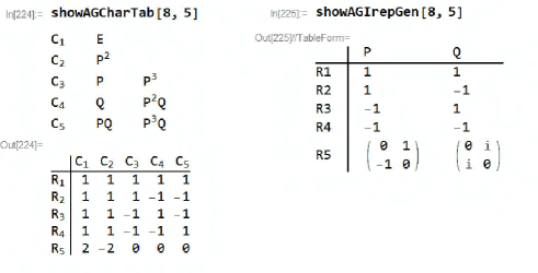
Figure 3: Examples of showAGCharTab[m,n] and showAGIrepGen[m,n] for the abstract group $G_{8}^{5}$.

6 Tables for LG IRs and SG IRs

6.1 Identify k-point

When the coordinates of a k-point are given, we have to know its name and its relation to the BC standard k-point before we can determine its LG IRs. In other words, we have to classify the k-point into one of the five types defined in subsection 2.3 and find the operation $\{S|\bm{w}\}$ if the k-point is of type II or III. There are two functions for doing this in SpaceGroupIrep, i.e.

⬇

identifyBCHSKpt[fullBZtype, kOrKlist]

identifyBCHSKptBySG[sgno, BZtypeOrBasVec, kOrKlist]

in which fullBZtype is the string code for one of the 22 types of BZs (see Tab. 1), kOrKlist is the numerical coordinates of a k-point or of a list of k-points, and BZtypeOrBasVec is either one of the BZtype in Tab. 1 or the numerical basic vectors of the space group. In fact, identifyBCHSKpt is a preprocessor of identifyBCHSKptBySG. The former identifies a k-point only according to BC-Tab. 3.6 without the SG information, while using the SG information the latter can further determine the $\{S|\bm{w}\}$ based on the results of the former.

The result returned by identifyBCHSKpt is a list

$$\{\bm{k},\text{\,kname},\,\text{\text{line\_info},\,}P(\bm{k}),\,\bm{k}_{{\rm BC}},\,S,\,S\bm{k}_{{\rm BC}},\,\bm{g},\ {\rm u}\rightarrow v_{{\rm u}}\}$$ (13)

where $\bm{k}$ is the k-point to be identified, kname is the identified name, line_info is the connection of HS line (null string if $\bm{k}$ is a HS point), $P(\bm{k})$ is the symmetry point group of $\bm{k}$ in the basic domain of the Bravais lattice, $\bm{k}_{{\rm BC}}$ is the BC standard k-point in the basic domain, $S$ is an element of $P(\bm{k})$ such that $\bm{k}\equiv S\bm{k}_{{\rm BC}}$, $\bm{g}=\bm{k}-S\bm{k}_{{\rm BC}}$ is the reciprocal lattice vector connecting $S\bm{k}_{{\rm BC}}$ and $\bm{k}$, and ${\rm u}\rightarrow v_{{\rm u}}$ is the rule for the actual value $v_{{\rm u}}$ of u. If kname is GP or UN only the first four items exist in Eq. (13), and the last item ${\rm u}\rightarrow v_{{\rm u}}$ exists only when $\bm{k}$ is on HS line. It is noteworthy that for multiple-BZ Bravais lattice, a k-point can be identified as two points with different names by identifyBCHSKpt, i.e. two entries in the form of Eq. (13) with different knames. And this case occurs when the k-point is on certain HS lines. For example, the k-point with coordinates $(-0.3,-0.3,0.3)$ is identified as $\Lambda$ in the BZ of type "TetrBody(b)" , while it is identified as either $\Lambda$ or $V$ in the BZ of type "TetrBody(a)". The code is as follow.

⬇

In[1]:= identifyBCHSKpt["TetrBody(b)",{-0.3,-0.3,0.3}]

identifyBCHSKpt["TetrBody(a)",{-0.3,-0.3,0.3}]

Out[1]= {{{-0.3,-0.3,0.3},$\Lambda$,$\Gamma$Z,C4v,{u,u,-u},C2x,{-u,-u,u},{0,0,0},u->0.3}}

Out[2]= {{{-0.3,-0.3,0.3},$\Lambda$,$\Gamma\Lambda$,C4v,{u,u,-u},C2x,{-u,-u,u},{0,0,0},u->0.3},

{{-0.3,-0.3,0.3},V,ZV,C4v,{-1/2+u,1/2+u,1/2-u},E,

{-1/2+u,1/2+u,1/2-u},{0,-1,0},u->0.2}}

Table 2: The table of $u_{{\rm max}}$ for HS lines, i.e. the maximum value of $u$ that keeps the BC standard k-point inside or on the boundary of the BZ. Except the HS lines in this table, the $u_{{\rm max}}$ of all other HS lines in BC-Tab. 3.6 is $\frac{1}{2}$. $a,b,c$ are lattice constants the same as those in BC-Tab. 3.1.

Type of BZ	$u_{{\rm max}}$ for HS lines
"OrthBase(a)"	$\Delta\text{: }\frac{1}{4}+\frac{b^{2}}{4a^{2}}$	$F\text{: }\frac{1}{4}-\frac{b^{2}}{4a^{2}}$	$B\text{: }\frac{1}{4}+\frac{b^{2}}{4a^{2}}$	$G\text{: }\frac{1}{4}-\frac{b^{2}}{4a^{2}}$
"OrthBase(b)"	$A\text{: }\frac{1}{4}+\frac{a^{2}}{4b^{2}}$	$E\text{: }\frac{1}{4}-\frac{a^{2}}{4b^{2}}$	$\Sigma\text{: }\frac{1}{4}+\frac{a^{2}}{4b^{2}}$	$C\text{: }\frac{1}{4}-\frac{a^{2}}{4b^{2}}$
"OrthBody(a)"	$\Lambda\text{: }\frac{1}{4}+\frac{c^{2}}{4a^{2}}$	$G\text{: }\frac{1}{4}-\frac{c^{2}}{4a^{2}}$	$\Delta\text{: }\frac{1}{4}+\frac{b^{2}}{4a^{2}}$	$U\text{: }\frac{1}{4}-\frac{b^{2}}{4a^{2}}$
"OrthBody(b)"	$\Lambda\text{: }\frac{1}{4}+\frac{c^{2}}{4b^{2}}$	$G\text{: }\frac{1}{4}-\frac{c^{2}}{4b^{2}}$	$\Sigma\text{: }\frac{1}{4}+\frac{a^{2}}{4b^{2}}$	$F\text{: }\frac{1}{4}-\frac{a^{2}}{4b^{2}}$
"OrthBody(c)"	$\Delta\text{: }\frac{1}{4}+\frac{b^{2}}{4c^{2}}$	$U\text{: }\frac{1}{4}-\frac{b^{2}}{4c^{2}}$	$\Sigma\text{: }\frac{1}{4}+\frac{a^{2}}{4c^{2}}$	$F\text{: }\frac{1}{4}-\frac{a^{2}}{4c^{2}}$
"OrthFace(a)"	$G\text{: }\frac{1}{4}+C_{ab}^{-}$	$H\text{: }\frac{1}{4}-C_{ab}^{-}$	$C\text{: }\frac{1}{4}+A_{bc}^{-}$	$A\text{: }\frac{1}{4}-A_{bc}^{-}$	$D\text{: }\frac{1}{4}+B_{ac}^{-}$	$B\text{: }\frac{1}{4}-B_{ac}^{-}$
"OrthFace(b)"	$\text{$\Lambda$}\text{: }\frac{1}{4}+C_{ab}^{+}$	$Q\text{: }\frac{1}{4}-C_{ab}^{+}$	$G\text{: }\frac{1}{4}+C_{ab}^{-}$	$H\text{: }\frac{1}{4}-C_{ab}^{-}$	$(C_{ab}^{\pm}=\frac{c^{2}(a^{2}\pm b^{2})}{4a^{2}b^{2}})$
"OrthFace(c)"	$\Delta\text{: }\frac{1}{4}+B_{ac}^{+}$	$R\text{: }\frac{1}{4}-B_{ac}^{+}$	$D\text{: }\frac{1}{4}+B_{ac}^{-}$	$B\text{: }\frac{1}{4}-B_{ac}^{-}$	$(B_{ac}^{\pm}=\frac{b^{2}(a^{2}\pm c^{2})}{4a^{2}c^{2}})$
"OrthFace(d)"	$\Sigma\text{: }\frac{1}{4}+A_{bc}^{+}$	$U\text{: }\frac{1}{4}-A_{bc}^{+}$	$C\text{: }\frac{1}{4}+A_{bc}^{-}$	$A\text{: }\frac{1}{4}-A_{bc}^{-}$	$(A_{bc}^{\pm}=\frac{a^{2}(b^{2}\pm c^{2})}{4b^{2}c^{2}})$
"TetrBody(a)"	$\Lambda\text{: }\frac{1}{4}+\frac{c^{2}}{4a^{2}}$	$V\text{: }\frac{1}{4}-\frac{c^{2}}{4a^{2}}$
"TetrBody(b)"	$\Sigma\text{: }\frac{1}{4}+\frac{a^{2}}{4c^{2}}$	$F\text{: }\frac{1}{4}-\frac{a^{2}}{4c^{2}}$	$U\text{: }\frac{1}{2}-\frac{a^{2}}{2c^{2}}$	$Y\text{: }\frac{a^{2}}{2c^{2}}$
"TrigPrim(a)"	$\Lambda\text{: }\frac{1}{6}+\frac{2c^{2}}{3a^{2}}$	$P\text{: }\frac{1}{3}-\frac{2c^{2}}{3a^{2}}$
"TrigPrim(b)"	$B\text{: }\frac{1}{3}-\frac{a^{2}}{6c^{2}}$	$Y\text{: }\frac{1}{6}+\frac{a^{2}}{6c^{2}}$	$\Sigma\text{: }\frac{1}{3}+\frac{a^{2}}{12c^{2}}$	$Q\text{: }\frac{1}{6}-\frac{a^{2}}{12c^{2}}$
"HexaPrim"	$T\text{: }\frac{1}{3}$	$T^{\prime}\text{: }\frac{1}{6}$	$S\text{: }\frac{1}{3}$	$S^{\prime}\text{: }\frac{1}{6}$
"CubiBody"	$\Lambda\text{: }\frac{1}{4}$	$F:\frac{1}{4}$
"CubiFace"	$\Sigma\text{: }\frac{3}{8}$	$S:\frac{1}{8}$

The information about a k-point from identifyBCHSKpt is preliminary. In the final result, the $\{S|\bm{w}\}$ defined in subsection 2.3 is determined and only one kname is determined with the knowledge of actual values of lattice constants or basic vectors. This is done by identifyBCHSKptBySG which returns the complete information of a k-point in the list form of

$$\{\bm{k},\text{\,kname},\,\text{\text{line\_info},\,}\bar{G}^{\bm{k}},\,\bm{k}_{{\rm BC}},\,\{S|\bm{w}\},\,S\bm{k}_{{\rm BC}},\,\bm{g},\ {\rm u}\rightarrow v_{{\rm u}},\,u_{{\rm max}},\,\text{if\/inG}\}$$ (14)

in which $\bar{G}^{\bm{k}}$ is the little co-group, $u_{{\rm max}}$ is the maximum value of $u$ that keeps $\bm{k}_{{\rm BC}}$ inside or on the boundary of the BZ, and ifinG is a string “in G” or “not in G” to indicate whether $\{S|\bm{w}\}\in G$ or not. In the above example, in order to determine whether the k-point $(-0.3,-0.3,0.3)$ is $\Lambda$ or $V$, the $u_{{\rm max}}$ of $\Lambda$ and $V$ should be known and then the one satisfying $v_{{\rm u}}<u_{{\rm max}}$ is selected. We can see that $u_{{\rm max}}$ depends on the actual values of lattice constants in most cases listed in Tab. 2. Therefore, the basic vectors are needed to precisely determine $\Lambda$ or $V$. Taking the space group $I4_{1}md$ (No. 109) for example, it has body-centered tetragonal lattice and has (a) type BZ when $a>c$. If $a=3$, $c=2$ then $u_{\max}^{\Lambda}=0.361111$ and $u_{\max}^{V}=0.138889$, which makes $0.3<u_{{\rm max}}^{\Lambda}$, $0.2>u_{{\rm max}}^{V}$ and then $\Lambda$ is selected. If $a=3$, $c=1$ then $u_{\max}^{\Lambda}=0.222222$ and $u_{\max}^{V}=0.277778$, which makes $0.3>u_{{\rm max}}^{\Lambda}$, $0.2<u_{{\rm max}}^{V}$ and then $V$ is selected. The code is as follow.

⬇

In[1]:= bv=BasicVectors["TetrBody"]

identifyBCHSKptBySG[109,bv/.{a->3,c->2},{-0.3,-0.3,0.3}]

identifyBCHSKptBySG[109,bv/.{a->3,c->1},{-0.3,-0.3,0.3}]

Out[1]= {{-a/2,a/2,c/2},{a/2,-a/2,c/2},{a/2,a/2,-c/2}}

Out[2]= {{-0.3,-0.3,0.3},$\Lambda$,$\Gamma\Lambda$,C4v,{u,u,-u},{C2x,{3/4,1/4,1/2}},

{-u,-u,u},{0,0,0},u->0.3,0.361111,not in G}

Out[3]= {{-0.3,-0.3,0.3},V,ZV,C4v,{-1/2+u,1/2+u,1/2-u},{E,{0,0,0}},

{-1/2+u,1/2+u,1/2-u},{0,-1,0},u->0.2,0.222222,in G}

When the basic vectors are unknown, we can use the BZtype, i.e. "a", "b", "c", "d", "", as the second parameter of identifyBCHSKptBySG. In this case, k-points on the HS lines listed in Tab. 2 except the last three rows may be identified with incorrect names, because the $u_{{\rm max}}$ cannot be determined precisely without actual values of $a,b,c$ and in this case $u_{{\rm max}}$ is set to a makeshift value $1/4$ to make sure only one kname is output. However, if $u_{{\rm max}}$ is not precisely determined and the option "allowtwok"->True is used, identifyBCHSKptBySG can still return two entries of k-point information with different knames for k-points on the HS lines in Tab. 2.

6.2 Tables for LG IRs

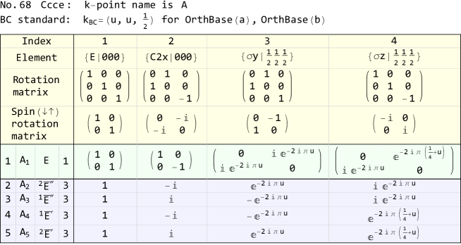
Figure 4: The output of the function showLGIrepTab[68,"A"] which shows the table for LG IRs of the k-point $A$ of the space group of number 68. Light green background shows single-valued IRs and light blue background shows double-valued IRs. Both the $\Gamma$ label (the second column) and the extended Mulliken label (the third column) are given. The first column is the index of the LG IRs and the fourth column is the realities whose values may be 1, 2, 3, or x.

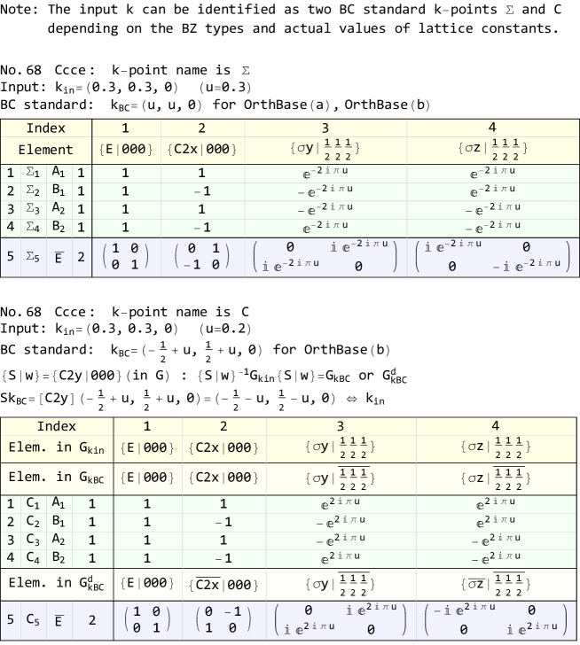
Figure 5: The output of the function showLGIrepTab[68,{0.3,0.3,0},"rotmat"->False] which shows two tables for LG IRs of the k-point $(0.3,0.3,0)$ of the space group of number 68. In this example $(0.3,0.3,0)$ is identified as two k-points $\Sigma$ and $C$, and which one is selected depends on the actual values of lattice constants. $k_{{\rm in}}$ means the input k-point, $G_{{\rm kin}}$ means the little group of $k_{{\rm in}}$, $G_{{\rm kBC}}$ means the little group of the standard BC k-point $k_{{\rm BC}}$, and $G_{{\rm kBC}}^{{\rm d}}$ means the double little group of $k_{{\rm BC}}.$

Although the data of LG IRs are contained in the BC book, they are distributed over several tables. This makes it not direct to obtain the representation matrices or characters of a designated LG IR, which is shown by the aforementioned example in the introduction. Accordingly, we create the functions getLGIrepTab[sgno,k] and showLGIrepTab[sgno,k] in which k is either the name or the numeric coordinates of a k-point. The former calculates and gives the representation matrices and related information of all the single-valued and double-valued LG IRs of k for the space group of number sgno, and the latter shows the data in user-friendly table form.

Fig. 4 is an example showing the output of showLGIrepTab[68,"A"] which directly gives the information about the k-point, the available types of BZ, the LG elements (only the coset representatives with respect to the translation group are given), the rotation matrices and spin rotation matrices, the representation matrices of both single-valued LG IRs (light green background) and double-valued LG IRs (light blue background), the $\Gamma$ labels ($A_{1},A_{2},\cdots$) and extended Mulliken labels ($E,$ ${}^{2}\!\bar{E}^{\prime\prime},\cdots$) of LG IRs, and the realities (the fourth column) of the corresponding SG IRs. Following the notations in the BC book, the realities 1, 2, 3 stand for real representation, pseudo-real representation, and complex representation respectively for the SG IRs in which $\bm{k}$ and $-\bm{k}$ are in the same star. If $\bm{k}$ and $-\bm{k}$ are not in the same star, the SG IR is complex and its reality is represented by a letter “x”. For double-valued LG IRs, the representation matrix of the element $\{\bar{R}|\bm{v}\}$ is just the negative value of the representation matrix of $\{R|\bm{v}\},$ so only $\{R|\bm{v}\}$’s are shown in the LG IR table in Fig. 4.

If the coordinates of a k-point are given, they may be identified as two BC standard k-points for the k-points listed in Tab. 2, and two LG IR tables are given by showLGIrepTab. An example of this case is showLGIrepTab[68,{0.3,0.3,0},"rotmat"->False] whose output is shown in Fig. 5. The input k-point $\bm{k}_{{\rm in}}=(0.3,0.3,0)$ is identified as only $\Sigma$ for "OrthBase(a)" type of BZ but as either $\Sigma$ or $C$ for "OrthBase(b)" type of BZ. Two LG IR tables for both $\Sigma$ and $C$ are given in Fig. 5. In this example, the coordinates $(0.3,0.3,0)$ are directly in the form of $(u,u,0)$, i.e. the coordinates of the BC standard $\Sigma$ k-point, and hence $\bm{k}_{{\rm in}}$ is of type I if it is a $\Sigma$ k-point. But if this k-point is identified as $C$, it is of type II and has non-identity $\{S|\bm{w}\}$ which can relate this k-point to the BC standard $C$ k-point. Here $\{S|\bm{w}\}=\{C_{2y}|000\}$ and it makes the little group of $\bm{k}_{{\rm in}}$, $G_{{\rm kin}}$, isomorphic to the (double) little group of $\bm{k}_{{\rm BC}}$, $G_{{\rm kBC}}$ ($G_{{\rm kBC}}^{{\rm d}}$), i.e.

$$\{S|\bm{w}\}^{-1}G_{{\rm kin}}\{S|\bm{w}\}=G_{{\rm kBC}}\ \ \text{or }G_{{\rm kBC}}^{{\rm d}}.$$ (15)

Then the LG IRs of $\bm{k}_{{\rm in}}$ are obtained from those of $\bm{k}_{{\rm BC}}$ according to Eqs. (11) and (15). The mappings between the elements in $G_{{\rm kin}}$ and those in $G_{{\rm kBC}}$ ($G_{{\rm kBC}}^{{\rm d}}$) are also shown in the lower table of Fig. 5, which can help to understand the relations between the LG IRs of $\bm{k}_{{\rm in}}$ and $\bm{k}_{{\rm BC}}.$ Let’s remind that here $\bm{k}_{{\rm in}}$ just borrows the name $C$ of $\bm{k}_{{\rm BC}}$ and if we give a different name to $\bm{k}_{{\rm in}},$ say $C^{\prime}$, then the LG IR labels of $\bm{k}_{{\rm in}}$ should be $C_{1}^{\prime},\cdots,C_{5}^{\prime}$ which are clearly distinguished from $C_{1},\cdots,C_{5}$ of $\bm{k}_{{\rm BC}}.$

Fig. 5 is generated by showLGIrepTab with the option "rotmat"->False which controls not to show the rotation matrices. In fact, showLGIrepTab has several options. Its default options can be obtained by

⬇

In[1]:= Options[showLGIrepTab]//InputForm

Out[1]= {"uNumeric"->False, "irep"->All, "elem"->All, "rotmat"->True,

"trace"->False, "spin"->"downup", "abcOrBasVec"->None,

"linewidth"-> 2}

If "uNumeric"->True is used, the value of $u$ is substituted into $u$ to make the LG IRs numeric. Although the LG IRs of $\Sigma$ and $C$ in Fig. 5 are different seemingly, it will be seen clearly that they are in fact equivalent when "uNumeric"->True is used, with the correspondence $\Sigma_{1,3}\leftrightarrow C_{3,1}$, $\Sigma_{2,4}\leftrightarrow C_{4,2}$, $\Sigma_{5}\leftrightarrow C_{5}.$ Options "irep" and "elem" can select certain IRs and elements to be shown, e.g. "irep"->{1,3},"elem"->{3,4} will only show the first and third LG IRs ($\Sigma_{1,3}$ and $C_{1,3}$ in Fig. 5) and the third and fourth elements ($\{\sigma_{y}|\frac{1}{2}\frac{1}{2}\frac{1}{2}\}$ and $\{\sigma_{z}|\frac{1}{2}\frac{1}{2}\frac{1}{2}\}$ in Fig. 5). "trace"->True makes showLGIrepTab show the characters not the representation matrices. In fact, we have also defined functions getLGCharTab[sgno,k] and showLGCharTab[sgno,k] to calculate and show the character tables for LG IRs and these two functions are just respectively the functions getLGIrepTab[sgno,k] and showLGIrepTab[sgno,k] with the option "trace"->True. The option "spin"->"updown" will change the bases of spin rotation matrices from the default $\{\downarrow,\uparrow\}$ to $\{\uparrow,\downarrow\}$. If lattice constants or basic vectors are given through the option "abcOrBasVec", one definite k-point is determined, e.g. "abcOrBasVec"->{a->3,b->5,c->4} only shows $\Sigma$ and "abcOrBasVec"->{a->2,b->5,c->4} only shows $C$ for the example in Fig. 5. At last, "linewidth" can control the line width of the table.

6.3 Tables for SG IRs

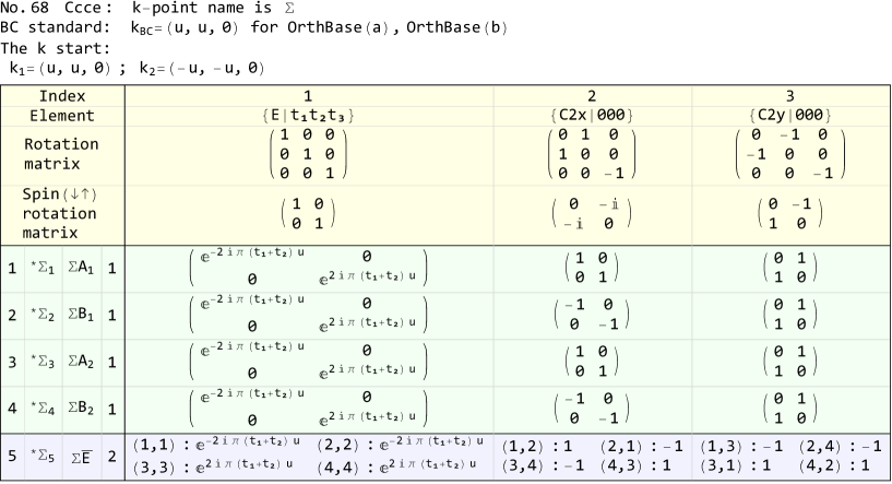
Figure 6: The output of showSGIrepTab[68,"$\Sigma$","maxDim"->3,"elem"->{1,2,3}] which shows part of the table for SG IRs of the star ${}^{*}\Sigma$ of the space group of number 68. Light green background shows single-valued IRs and light blue background shows double-valued IRs. The first column is the index of the SG IRs, the second and third column are two kinds of labels for SG IRs, and the fourth column is the realities whose values may be 1, 2, 3, or x.

In addition to tables for LG IRs, we have also created the functions getSGIrepTab[sgno,k] and showSGIrepTab[sgno,k] to calculate and show the tables for SG IRs. The usage of showSGIrepTab[sgno,k] is almost the same as showLGIrepTab[sgno,k] except that showSGIrepTab has one more option "maxDim". "maxDim" is the critical dimension controlling the appearance of representations whose default value is 4. When the dimension of a representation matrix is lower than or equal to "maxDim" , the representation matrix is shown in matrix form, and otherwise only nonzero matrix elements are shown to save the table space. An example is shown in Fig. 6, which is generated by the following code.

⬇

showSGIrepTab[68, "$\Sigma$", "maxDim"->3, "elem"->{1,2,3}]

This example gives the table for the SG IRs of the wave vector star ${}^{*}\Sigma$ of space group 68. The double-valued SG IR ${}^{*}\Sigma_{5}$ is shown in the form of nonzero matrix elements, because its dimension 4 is larger than the value 3 of "maxDim". To save space, representation matrices of only the first three SG elements are shown due to the option "elem"->{1,2,3}. If the option "elem" is not used, the table will show the representation matrices of 8 SG elements in total, i.e. all the coset representatives with respective to the translation group. We use two kinds of labels for SG IRs. The first one is to put a $*$ at the top left corner of corresponding $\Gamma$ label of LG IR, and the second one is to put the k-point name in front of the extended Mulliken label of LG IR, e.g. both ${}^{*}\Sigma_{2}$ and $\Sigma B_{1}$ for $\Sigma_{2}\uparrow G$.

7 Direct product of SG IRs

The (inner) direct product of SG IRs is of great importance to determine the selection rules in various quantum processes in crystals. Therefore we have realized the decomposition (or reduction) of the direct product of any two SG IRs according to BC-Eqs. (4.7.1) and (4.7.29), i.e.

$$(\Gamma_{p}^{i}\uparrow G)\otimes(\Gamma_{q}^{j}\uparrow G)\equiv\sum_{l}\sum_{r}C_{pq,r}^{ij,l}(\Gamma_{r}^{l}\uparrow G)$$ (16)

$$C_{pq,r}^{ij,l}=\sum_{\{\alpha|\bm{u}\}}\!\!\vphantom{\sum}^{\prime}\sum_{\{\beta|\bm{v}\}}\!\!\vphantom{\sum}^{\prime}\frac{|T|}{|N_{\alpha\beta}|}\sum_{\{\gamma|\bm{w}\}\in N_{\alpha\beta}/T}\chi_{p}^{i}(\{\beta|\bm{v}\}^{-1}\{\gamma|\bm{w}\}\{\beta|\bm{v}\})\cdot\chi_{q}^{j}(\{\alpha|\bm{u}\}\{\gamma|\bm{w}\}\{\alpha|\bm{u}\})\cdot\chi_{r}^{l*}(\{\gamma|\bm{w}\})$$ (17)

in which $\sum\vphantom{\sum}^{\prime}$ means the summation is restricted by the condition

$$\beta\bm{k}_{i}+\alpha\bm{k}_{j}\equiv\bm{k}_{l}.$$ (18)

In the above equations, $\Gamma_{p}^{i}$, $\Gamma_{q}^{j},$ and $\Gamma_{r}^{l}$ are the LG IRs of the little groups $G^{\bm{k}_{i}}$, $G^{\bm{k}_{j}},$ and $G^{\bm{k}_{l}}$ respectively; $\chi_{p}^{i},$ $\chi_{q}^{j},$ and $\chi_{r}^{l}$ are their characters respectively; and $\Gamma_{p}^{i}\uparrow G$, $\Gamma_{q}^{j}\uparrow G$, and $\Gamma_{r}^{l}\uparrow G$ are the corresponding induced SG IRs of the space group $G$. $\{\alpha|\bm{u}\}$’s are the double coset representatives of $G$ with respect to $G^{\bm{k}_{l}}$ and $G^{\bm{k}_{j}}$; $\{\beta|\bm{v}\}$’s are the double coset representatives of $G$ with respect to $L_{\alpha}=G^{\bm{k}_{l}}\cap(\{\alpha|\bm{u}\}G^{\bm{k}_{j}}\{\alpha|\bm{u}\}^{-1})$ and $G^{\bm{k}_{i}}$; and $N_{\alpha\beta}$ is a group defined by $N_{\alpha\beta}=L_{\alpha}\cap(\{\beta|\bm{v}\}G^{\bm{k}_{i}}\{\beta|\bm{v}\}^{-1})$.

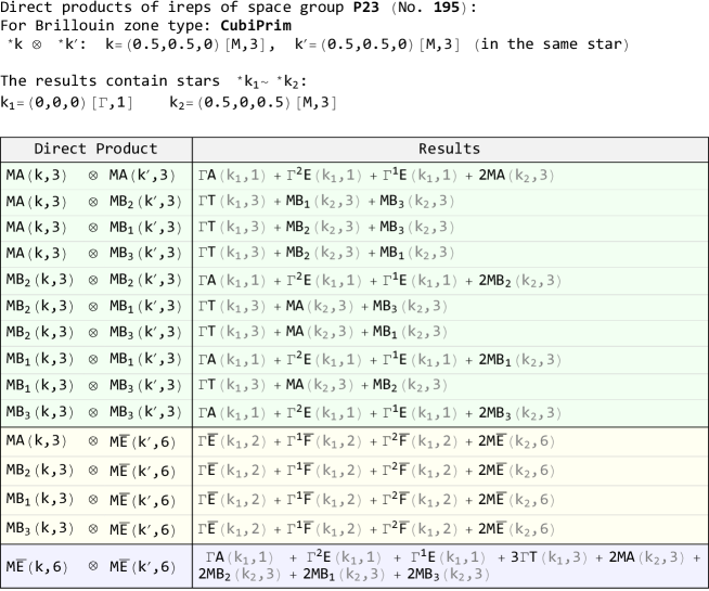
Figure 7: The output of showSGIrepDirectProduct[195, {1/2,1/2,0}, {1/2,1/2,0}, "label"->2] which shows the direct product of SG IRs of ${}^{*}M$ and ${}^{*}M$ for space group $P23$. The notation $[M,3]$ on top of the table means the the k-point in front of it is identified as $M$ and the number of arms of its star is 3. The notation $(k_{2},3)$ in the table indicates that the SG IR in front of it is for the star of $k_{2}$ and the dimension of this SG IR is 3. Light green background stands for direct products between single-valued SG IRs and single-valued SG IRs, light yellow background for direct products between single-valued SG IRs and double-valued SG IRs, and light blue background for direct products between double-valued SG IRs and double-valued SG IRs.

The functions that calculate and show the direct product of SG IRs are SGIrepDirectProduct[sgno,k1,k2] and showSGIrepDirectProduct[sgno,k1,k2] respectively, in which k1 and k2 are both numeric k-point coordinates. Taking the same example as in the BC book, that is the direct products of SG IRs of ${}^{*}M$ and ${}^{*}M$ for space group $P23$ (No. 195). The following function

⬇

showSGIrepDirectProduct[195, {1/2,1/2,0}, {1/2,1/2,0}, "label"->2]

gives the results shown in Fig. 7, which are consistent with the direct products listed in BC-Tab. 4.5. showSGIrepDirectProduct has three options, "label", "abcOrBasVec", and "linewidth", in which "label" whose value can be 1 (default) or 2 controls which kind of labels for SG IRs are used and the other two options have the same usages as in showLGIrepTab. It is worth noting that showSGIrepDirectProduct not only gives the direct products between single-valued SG IRs and single-valued SG IRs, but also gives the direct products between double-valued SG IRs and double-valued SG IRs and even direct products between single-valued SG IRs and double-valued SG IRs.

8 Obtain the LG IRs of energy bands

As mentioned in the introduction, a tool with full support for determining the LG IRs of all Bloch states in energy bands has been missing for a long time until the appearance of the recent program irvsp[41]. However, irvsp only supports LG IRs in the BCS convention. Therefore, support for LG IRs in the BC convention is provided in the SpaceGroupIrep package, as a complement to irvsp.

Here, we use “BC cells” for the primitive cells with BC settings, i.e. the cells have basic vectors defined in BC-Tab. 3.1 and the SG symmetry operations defined by the cells are consistent with the first-row generators of every space group in BC-Tab. 3.7. Note that a cell only with basic vectors defined in BC-Tab. 3.1 is not necessary a BC cell, because different selections for the origin may result in different SG elements. In the following two subsections, we first discuss the cases with BC cells, and then discuss the cases with non-BC cells.

8.1 For BC cells

To determine the LG IRs of energy bands, the character of each LG element operating on each set of degenerate Bloch states should be obtained first. Fortunately, there has be such a program called vasp2trace[27] which can do this. vasp2trace is a third-party post-processing program for VASP. It reads the output wave functions of VASP, calculates the characters of LG elements, and writes the results in a file named trace.txt. In fact, vasp2trace is the precursor of irvsp without the function of determining LG IRs and irvsp can also output a trace.txt file in certain cases. However, the trace.txt files generated by the two programs may be different and what we need is the trace.txt generated by vasp2trace, because the chacracter data in the trace.txt file from irvsp may be processed data, not the original ones we need. It is worth noting that the number of bands output by vasp2trace is limited by the number of electrons, i.e. the NELECT in VASP, because vasp2trace is designed for determining the topological properties of materials and for this purpose only the trace data of occupied states are needed. To make vasp2trace output trace data for all bands, two tiny changes should be made to the source code of vasp2trace: changing the nele in the 30th line of wrtir.f90 to ne and deleting the 55th line of chrct.f90, i.e. IF(IE>nele) EXIT.

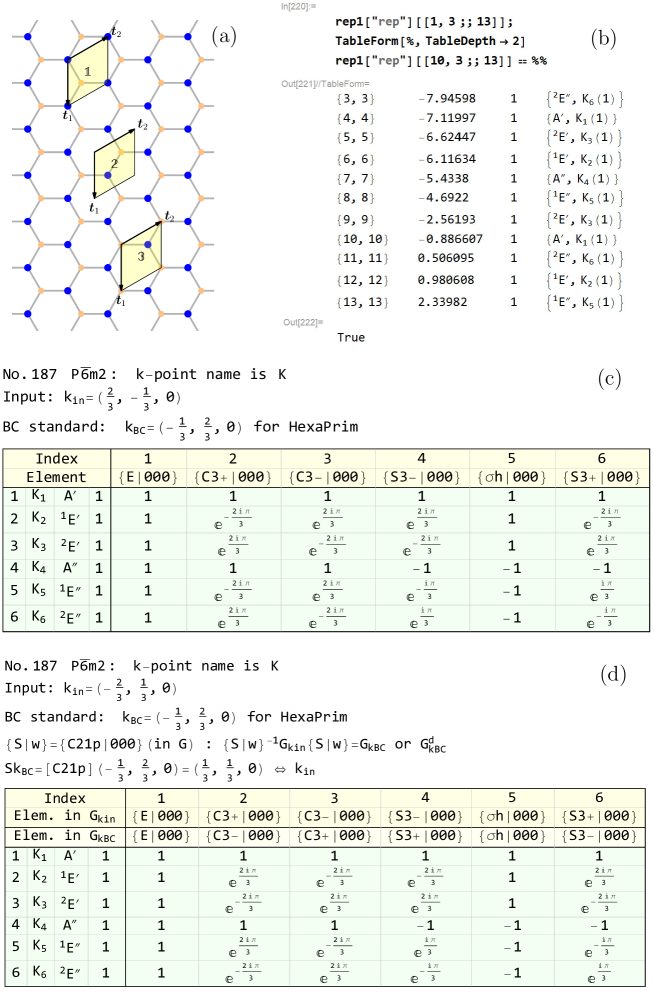
Figure 8: The LG IRs of monolayer MoS₂. (a) Top view and three different BC cells for monolayer MoS₂ where blue and orange dots represent Mo and S atoms respectively. (b) Codes to show the LG IRs at $K$ (the first k-point) and $K^{\prime}$ (the 10th k-point) for seven valence bands (3–9) and four conduction bands (10–13). The four columns of the output are respectively the range of bands for a degenerate energy (e.g. {3,3} means from band 3 to band 3), the band energy, the degree of degeneracy, and the labels for LG IRs. Both the extended Mulliken label and the $\Gamma$ label for a LG IR are given and the integer in the parentheses is the dimension of the LG IR. (c) The character table for LG IRs of $K$ $(\frac{2}{3},-\frac{1}{3},0)$ obtained by showLGCharTab[187,{2/3,-1/3,0},"rotmat"->False,"irep"->1;;6]. (d) The character table for LG IRs of $K^{\prime}$ $(-\frac{2}{3},\frac{1}{3},0)$ obtained by showLGCharTab[187,{-2/3,1/3,0},"rotmat"->False,"irep"->1;;6].

In the SpaceGroupIrep package we use the function readVasp2trace to read the trace.txt file generated by vasp2trace and its returned value is an association containing all the data in the trace.txt file. Then the function getBandRep is used to determine the LG IRs according to the trace data returned by readVasp2trace. There are three ways to call getBandRep, i.e.

⬇

getBandRep[sgno, BZtypeOrBasVec, traceData]

getBandRep[sgno, BZtypeOrBasVec, traceData, ikOrListOrSpan]

getBandRep[sgno, BZtypeOrBasVec, traceData, ikOrListOrSpan, ibOrListOrSpan]

in which BZtypeOrBasVec has the same meaning as in identifyBCHSKptBySG, traceData is the value returned by readVasp2trace, ikOrListOrSpan (ibOrListOrSpan) specifies the indexes of k-points (bands) to be processed. ikOrListOrSpan (ibOrListOrSpan) may be an integer such as 5, a list of integers such as {2,3,5}, or a span such as 3;;5. If ikOrListOrSpan (ibOrListOrSpan) is not specified then all k-points (bands) are processed. Taking monolayer MoS₂ (space group 187) for example, we calculate its energy bands by VASP using the unit cell 1 shown in Fig. 8(a), get trace.txt file by vasp2trace, and then determine the LG IRs for all Bloch states in the bands by

⬇

(* put trace.txt to the current working directory *)

tr1=readVasp2trace["trace.txt"];

rep1=getBandRep[187, "", tr1];

in which rep1 is an association having keys "kpath", "rep", and "kinfo", and the determined LG IRs are contained in rep1["rep"]. In this example, the first k-point is $K$ $(\frac{2}{3},-\frac{1}{3},0)$ and the 10th k-point is $K^{\prime}$ $(-\frac{2}{3},\frac{1}{3},0)$. Then the LG IRs of $K$ for seven valence bands 3–9 and four conduction bands 10–13 can be extracted by rep1["rep"][[1, 3;;13]] whose result is shown in Fig. 8(b). The $\Gamma$ labels $K_{1}\sim K_{6}$ of LG IRs in Fig. 8(b) should refer to the character table in Fig. 8(c), from which it can be seen that the characters of $C_{3}^{+}$ and $\sigma_{h}$ are consistent with the data listed in the Tab. 2 of ref. [45]. It should be pointed out that the LG IRs of $K^{\prime}$, i.e. the results of rep1["rep"][[10, 3;;13]], are seemingly the same with $K$ as shown by the “True” in Fig. 8(b). However, the meanings of $K_{1}\sim K_{6}$ are different because the LG IRs for $K^{\prime}$ should refer to the character table in Fig. 8(d). Taking the topmost valence band (the 9th band) as example, the character of $\{C_{3}^{+}|000\}$ for the $K_{3}$ of $K$ is $e^{i\frac{2\pi}{3}}$ [c.f. Fig. 8(c)], but the character of $\{C_{3}^{+}|000\}$ for the $K_{3}$ of $K^{\prime}$ is $e^{-i\frac{2\pi}{3}}$ [c.f. Fig. 8(d)]. The two characters are complex conjugates of each other, which is consistent with the time reversal symmetry between the states of $K$ and $K^{\prime}$. Because $K^{\prime}$ is not a BC standard k-point, we should remember that it borrows the name $K$ from its related BC standard k-point. In fact, if a non-BC k-point has its own name, we can directly use this name in its labels of LG IRs, e.g. the $K_{1}\sim K_{6}$ in Fig. 8(d) are in fact $K_{1}^{\prime}\sim K_{6}^{\prime}$.

It is noteworthy that the BC cell of a crystal is probably not unique. Also taking monolayer MoS₂ for example, the three cells in Fig. 8(a) are all BC cells, but they have different origins. Consequently, the LG IR of a certain state is different for the three different cells, because the rotation center is different, e.g. the LG IRs of the topmost valence band and the lowest conduction band (the 10th band) at $K$ for the three BC cells can be obtained as follow

⬇

In[1]:= rep1["rep"][[1, 9;;10]]//TableForm[#,TableDepth->2]&

rep2["rep"][[1, 9;;10]]//TableForm[#,TableDepth->2]&

rep3["rep"][[1, 9;;10]]//TableForm[#,TableDepth->2]&

Out[1]= {9,9} -2.56193 1 {²E^′, K₃(1)}

{10,10} -0.886607 1 {A^′, K₁(1)}

Out[2]= {9,9} -2.56193 1 {A^′, K₁(1)}

{10,10} -0.886609 1 {¹E^′, K₂(1)}

Out[3]= {9,9} -2.56188 1 {¹E^′, K₂(1)}

{10,10} -0.886553 1 {²E^′, K₃(1)}

in which rep1, rep2, and rep3 are the returned values of getBandRep for BC cells 1, 2, and 3 in Fig. 8(a) respectively. The LG IRs for the three BC cells are consistent with the eigenvalues of $C_{3}^{+}$ in the Tab. 2 of ref. [45] for three different rotation centers. Therefore, if the primitive cell is not given explicitly, we cannot say what is the LG IR of the topmost valence band at $K$ (or any other state) for monolayer MoS₂.

8.2 For non-BC cells

For a non-BC primitive cell, it has to be converted to a BC cell and its trace data also has to be converted accordingly before determining LG IRs. To convert cells, we adopt the conventions used in the package spglib. In spglib, converting one cell to another needs three ingredients, i.e. transformation matrix, rotation matrix, and origin shift[46]. Concretely speaking, spglib can convert any input cell with basic vectors $\bm{a}_{0}$, $\bm{b}_{0}$, and $\bm{c}_{0}$ to an idealized standard cell with basic vectors $\bm{a}_{s}^{\prime}$, $\bm{b}_{s}^{\prime}$, and $\bm{c}_{s}^{\prime}$ through the relation

$$(\bm{a}_{s}^{\prime},\bm{b}_{s}^{\prime},\text{$\bm{c}_{s}^{\prime})=R_{{\rm std}}(\bm{a}_{0},s\bm{b}_{0},\bm{c}_{0})$}P^{-1},$$ (19)

in which $P$ and $R_{{\rm std}}$ are respectively the transformation matrix and rotation matrix determined by spglib. The above basic vectors are all column matrices, so both $(\bm{a}_{0},\bm{b}_{0},\bm{c}_{0})$ and $(\bm{a}_{s}^{\prime},\bm{b}_{s}^{\prime},\bm{c}_{s}^{\prime})$ are $3\times 3$ square matrices and called “basic-vector matrix”. In the conventions of spglib, transformation matrix makes linear combination of basic vectors to form new basic vectors but does not rotate the crystal, while rotation matrix rotates the crystal and hence rotates all basic vectors. Therefore, transformation matrix is always multiplied on the right side of a basic-vector matrix, while rotation matrix is always multiplied on the left side of a basic-vector matrix. Further using the origin shift $\bm{p}$ determined by spglib, the atomic coordinates and SG elements can be converted as follow

$$\bm{x}_{0}\ \ \ \ \rightarrow\ \ \ \ \bm{x}_{s}=P\bm{x}_{0}+\bm{p},$$ (20)

$$\{R_{0}|\bm{v}_{0}\}\ \ \ \ \rightarrow\ \ \ \ \{R_{s}|\bm{v}_{s}\}=\{PR_{0}P^{-1}|P\bm{v}_{0}-R_{s}\bm{p}+\bm{p}\},$$ (21)

in which $\bm{x}_{0}$ and $\{R_{0}|\bm{v}_{0}\}$ are respectively the atomic coordinates and SG elements of the input cell, and $\bm{x}_{s}$ and $\{R_{s}|\bm{v}_{s}\}$ are respectively the atomic coordinates and SG elements of the idealized standard cell of spglib. In fact, the idealized standard cell of spglib is the conventional cell consistent with the first setting of ITA[43] and hence can also be called “ITA cell”.

Table 3: Changes to BC-Tab. 3.7. All space groups that are not listed in this table have the same data for the original BC-Tab. 3.7 and the adapted BC-Tab. 3.7.

No.	Symbol	Generators	$\bm{t}_{0}$
68	$Ccca$	{$C_{2x}|000\},\ \{C_{2y}|000\},\ \{I|\frac{1}{2}\frac{1}{2}\frac{1}{2}\}$	0
125	$P4/nbm$	{$C_{4z}^{+}|\frac{1}{2}\frac{1}{2}0\},\ \{C_{2x}|000\},\ \{I|\frac{1}{2}\frac{1}{2}0\}$	$\frac{1}{2}\bm{t}_{1}$
		{$C_{4z}^{+}|000\},\ \{C_{2x}|000\},\ \{I|\frac{1}{2}\frac{1}{2}0\}$
141	$I4_{1}/amd$	{$C_{4z}^{+}|0\frac{1}{2}0\},\ \{C_{2x}|\frac{1}{2}\frac{1}{2}0\},\ \{I|\frac{1}{2}\frac{1}{2}0\}$	$\frac{3}{8}\bm{t}_{1}+\frac{1}{8}\bm{t}_{2}+\frac{1}{4}\bm{t}_{3}$
		{$C_{4z}^{+}|\frac{3}{4}\frac{1}{4}\frac{1}{2}\},\ \{C_{2x}|\frac{3}{4}\frac{1}{4}\frac{1}{2}\},\ \{I|\frac{3}{4}\frac{1}{4}\frac{1}{2}\}$
142	$I4_{1}/acd$	{$C_{4z}^{+}|\frac{1}{2}00\},\ \{C_{2x}|\frac{1}{2}\frac{1}{2}0\},\ \{I|000\}$	$\frac{1}{8}\bm{t}_{1}+\frac{3}{8}\bm{t}_{2}-\frac{1}{4}\bm{t}_{3}$
		{$C_{4z}^{+}|\frac{3}{4}\frac{1}{4}\frac{1}{2}\},\ \{C_{2x}|\frac{1}{4}\frac{3}{4}\frac{1}{2}\},\ \{I|\frac{3}{4}\frac{1}{4}\frac{1}{2}\}$
155	$R32$	{$C_{3}^{+}|000\},\ \{C_{21}^{\prime}|000\}$	0
160	$R3m$	{$C_{3}^{+}|000\},\ \{\sigma_{d1}|000\}$	0
161	$R3c$	{$C_{3}^{+}|000\},\ \{\sigma_{d1}|\frac{1}{2}\frac{1}{2}\frac{1}{2}\}$	0
166	$R\bar{3}m$	{$S_{6}^{+}|000\},\ \{\sigma_{d1}|000\}$	0
167	$R\bar{3}c$	{$S_{6}^{+}|000\},\ \{\sigma_{d1}|\frac{1}{2}\frac{1}{2}\frac{1}{2}\}$	0
178	$P6_{1}22$	{$C_{6}^{+}|00\frac{1}{6}\},\ \{C_{21}^{\prime}|000\}$	$\frac{1}{4}\bm{t}_{3}$
		{$C_{6}^{+}|00\frac{1}{6}\},\ \{C_{21}^{\prime\prime}|000\}$
179	$P6_{5}22$	{$C_{6}^{+}|00\frac{5}{6}\},\ \{C_{21}^{\prime}|000\}$	$\frac{1}{4}\bm{t}_{3}$
		{$C_{6}^{+}|00\frac{5}{6}\},\ \{C_{21}^{\prime\prime}|000\}$
182	$P6_{3}22$	{$C_{6}^{+}|00\frac{1}{2}\},\ \{C_{21}^{\prime}|000\}$	$\frac{1}{4}\bm{t}_{3}$
		{$C_{6}^{+}|00\frac{1}{2}\},\ \{C_{21}^{\prime\prime}|000\}$

Next, we should convert the ITA cell to a BC cell with the aid of BC-Tab. 3.7. BC-Tab. 3.7 gives the SG generators of each space group and for some space groups there are two rows of data of which the first-row generators are the ones used in the BC book and the second-row generators are those used in the book [47] (referred to as IT1965 hereafter) but based on the BC basic vectors. Then we call the cell having the second-row SG generators “second-row cell”, and in this sense a BC cell is just a “first-row cell”. If a space group has only one row of generators in BC-Tab. 3.7, the term second-row cell can also be used but has the same meaning as the first-row cell. In fact, IT1965 can be considered as an earlier edition of ITA but their SG settings have some differences. In order to convert the ITA cell to a BC cell, BC-Tab. 3.7 has to be adapted and the changes are listed in Tab. 3. So the BC-Tab. 3.7 with the changes in Tab. 3 is called “the adapted BC-Tab. 3.7”.

Figure 9: The procedure of converting the input cell to the BC cell. The transformation matrices (red color) and rotation matrices (blue color) are shown above the arrows, and the origin shifts (if exist) are shown below the arrows.

According to the adapted BC-Tab. 3.7, we first convert the ITA cell to a second-row cell, and then convert the second-row cell to a BC cell. The first conversion has the transformation matrix $Q$, rotation matrix $S_{1}$ and no origin shift, and the second conversion has the transformation matrix $U$, rotation matrix $S_{2}$, and origin shift $\bm{t}_{0}$. Suppose that the basic-vector matrices of the second-row cell and the BC cell are $(\bm{t}_{1}^{\prime(2)},\bm{t}_{2}^{\prime(2)},\bm{t}_{3}^{\prime(2)})$ and $(\bm{t}_{1},\bm{t}_{2},\bm{t}_{3})$ respectively, that the atomic coordinates of the two cells are $\bm{x}^{(2)}$ and $\bm{x}$ respectively, and that the SG elements of the two cells are $\{R^{(2)}|\bm{v}^{(2)}\}$ and $\{R|\bm{v}\}$ respectively. Then the conversion from the ITA cell to the second-row cell consists of the following relations

$$(\bm{t}_{1}^{\prime(2)},\bm{t}_{2}^{\prime(2)},\bm{t}_{3}^{\prime(2)})=S_{1}(\bm{a}_{s}^{\prime},\bm{b}_{s}^{\prime},\bm{c}_{s}^{\prime})Q,$$ (22)

$$\bm{x}_{s}\ \ \ \ \rightarrow\ \ \ \ \bm{x}^{(2)}=Q^{-1}\bm{x}_{s},$$ (23)

$$\{R_{s}|\bm{v}_{s}\}\ \ \ \ \rightarrow\ \ \ \ \{R^{(2)}|\bm{v}^{(2)}\}=\{Q^{-1}R_{s}Q\,|\,Q^{-1}\bm{v}_{s}\},$$ (24)

and the conversion from the second-row cell to the BC cell consists of the following relations

$$(\bm{t}_{1},\bm{t}_{2},\bm{t}_{3})=S_{2}(\bm{t}_{1}^{\prime(2)},\bm{t}_{2}^{\prime(2)},\bm{t}_{3}^{\prime(2)})U,$$ (25)

$$\bm{x}^{(2)}\ \ \ \ \rightarrow\ \ \ \ \bm{x}=U^{-1}\bm{x}^{(2)}+\bm{t}_{0},$$ (26)

$$\{R^{(2)}|\bm{v}^{(2)}\}\ \ \ \ \rightarrow\ \ \ \ \{R|\bm{v}\}=\{U^{-1}R^{(2)}U\,|\,U^{-1}\bm{v}^{(2)}-R\bm{t}_{0}+\bm{t}_{0}\},$$ (27)

where $\bm{t}_{0}$ is given in the adapted BC-Tab. 3.7.

Table 4: The transformation matrix $Q$ and rotation matrix $S_{1}$ in Eq. (22) for each Bravais lattice. ${\rm c}\gamma$ (${\rm s}\gamma$) means $\cos\gamma$ ($\sin\gamma$) and $\gamma$ is the non-right angle between basic vectors of monoclinic lattices given in BC-Tab. 3.1.

Bravais lattice	$Q$	$S_{1}$	Bravais lattice	$Q$	$S_{1}$
⬇ TetrPrim				$\begin{bmatrix}1&0&0\\ 0&1&0\\ 0&0&1\end{bmatrix}$	$\begin{bmatrix}1&0&0\\ 0&1&0\\ 0&0&1\end{bmatrix}$
⬇ TetrBody				$\begin{bmatrix}-\frac{1}{2}&\frac{1}{2}&\frac{1}{2}\\ \frac{1}{2}&-\frac{1}{2}&\frac{1}{2}\\ \frac{1}{2}&\frac{1}{2}&-\frac{1}{2}\end{bmatrix}$	$\begin{bmatrix}1&0&0\\ 0&1&0\\ 0&0&1\end{bmatrix}$
⬇ TrigPrim				$\begin{bmatrix}\frac{2}{3}&-\frac{1}{3}&-\frac{1}{3}\\ \frac{1}{3}&\frac{1}{3}&-\frac{2}{3}\\ \frac{1}{3}&\frac{1}{3}&\frac{1}{3}\end{bmatrix}$	$\begin{bmatrix}-\frac{1}{2}&\frac{\sqrt{3}}{2}&0\\ -\frac{\sqrt{3}}{2}&-\frac{1}{2}&0\\ 0&0&1\end{bmatrix}$
⬇ HexaPrim				$\begin{bmatrix}1&0&0\\ 0&1&0\\ 0&0&1\end{bmatrix}$	$\begin{bmatrix}0&1&0\\ -1&0&0\\ 0&0&1\end{bmatrix}$
⬇ CubiPrim				$\begin{bmatrix}1&0&0\\ 0&1&0\\ 0&0&1\end{bmatrix}$	$\begin{bmatrix}1&0&0\\ 0&1&0\\ 0&0&1\end{bmatrix}$
⬇ CubiFace				$\begin{bmatrix}0&\frac{1}{2}&\frac{1}{2}\\ \frac{1}{2}&0&\frac{1}{2}\\ \frac{1}{2}&\frac{1}{2}&0\end{bmatrix}$	$\begin{bmatrix}1&0&0\\ 0&1&0\\ 0&0&1\end{bmatrix}$
⬇ CubiFace				$\begin{bmatrix}-\frac{1}{2}&\frac{1}{2}&\frac{1}{2}\\ \frac{1}{2}&-\frac{1}{2}&\frac{1}{2}\\ \frac{1}{2}&\frac{1}{2}&-\frac{1}{2}\end{bmatrix}$	$\begin{bmatrix}1&0&0\\ 0&1&0\\ 0&0&1\end{bmatrix}$

To sum up briefly, any input cell can be converted to BC cell via two intermediate cells and the procedure includes three steps: firstly input cell to ITA cell, then ITA cell to second-row cell, and lastly second-row cell to BC cell, as shown in Fig. 9. In the first step, $R_{{\rm std}}$, $P$, and $\bm{p}$ are all determined by spglib; in the second step, $Q$ and $S_{1}$ are listed in Tab. 4 according to the Bravais lattice of space group; and in the last step, $U$ and $S_{2}$ are listed in Tab. 5 and $\bm{t}_{0}$ is given in the last column of the adapted BC-Tab. 3.7. Integrating the three steps from Eq. (19) to Eq. (27), the integrated conversion from the input cell to the BC cell consists of the following relations

$$(\bm{t}_{1},\bm{t}_{2},\bm{t}_{3})=S_{2}S_{1}R_{{\rm std}}(\bm{a}_{0},\bm{b}_{0},\bm{c}_{0})P^{-1}QU,$$ (28)

$$\bm{x}_{0}\ \ \ \ \rightarrow\ \ \ \ \bm{x}=U^{-1}Q^{-1}(P\bm{x}_{0}+\bm{p})+\bm{t}_{0},$$ (29)

$$\{R_{0}|\bm{v}_{0}\}\ \ \ \ \rightarrow\ \ \ \ \{R|\bm{v}\}\begin{cases}R=U^{-1}Q^{-1}PR_{0}P^{-1}QU\\ \bm{v}=U^{-1}Q^{-1}(P\bm{v}_{0}-PR_{0}P^{-1}\bm{p}+\bm{p})-R\bm{t}_{0}+\bm{t}_{0}\end{cases}.$$ (30)

Table 5: The transformation matrix $U$ and rotation matrix $S_{2}$ in Eq. (25) for the space groups with an $*$ in the last column of the adapted BC-Tab. 3.7. The BC book uses orientations different from the default ones in ITA for these space groups, and the orientations used are given here in the second column (refer to ITA for the meanings of the orientations). For the space groups not listed in this table, both $U$ and $S_{2}$ are identity matrix.

Space Group		orientation	$U$	$S_{2}$
$17\ (P222_{1})$	$19\ (P2_{1}2_{1}2_{1})$	$\bm{b\bar{a}c}$	$\begin{bmatrix}\begin{array}[]{ccc}0&-1&0\\ 1&0&0\\ 0&0&1\end{array}\end{bmatrix}$	$\begin{bmatrix}0&1&0\\ -1&0&0\\ 0&0&1\end{bmatrix}$
$28\ (Pma2)$	$29\ (Pca2_{1})$
$31\ (Pmn2_{1})$	$33\ (Pna2_{1})$
$53\ (Pmna)$	$61\ (Pbca)$
$36\ (Cmc2_{1})$			$\begin{bmatrix}\begin{array}[]{ccc}0&-1&0\\ 1&0&0\\ 0&0&1\end{array}\end{bmatrix}$
$46\ (Ima2)$			$\begin{bmatrix}\begin{array}[]{ccc}0&1&0\\ 0&1&-1\\ -1&1&0\end{array}\end{bmatrix}$
$70\ (Fddd)$			$\begin{bmatrix}\begin{array}[]{ccc}1&1&1\\ 0&0&-1\\ -1&0&0\end{array}\end{bmatrix}$
$122\ (I\bar{4}2d$)			$\begin{bmatrix}\begin{array}[]{ccc}0&1&0\\ 0&1&-1\\ -1&1&0\end{array}\end{bmatrix}$
38 $(Amm2)$ 40 $(Ama2)$	39 $(Abm2)$ 41 $(Aba2)$	$\bm{bca}$	$\begin{bmatrix}\begin{array}[]{ccc}-1&0&0\\ 0&0&1\\ 0&1&0\end{array}\end{bmatrix}$	$\begin{bmatrix}0&1&0\\ 0&0&1\\ 1&0&0\end{bmatrix}$
$57\ (Pbcm)$			$\begin{bmatrix}\begin{array}[]{ccc}0&-1&0\\ 0&0&1\\ -1&0&0\end{array}\end{bmatrix}$
$51\ (Pmma)$	$54\ (Pcca)$	$\bm{\bar{c}ba}$	$\begin{bmatrix}\begin{array}[]{ccc}1&0&0\\ 0&0&1\\ 0&-1&0\end{array}\end{bmatrix}$	$\begin{bmatrix}0&0&-1\\ 0&1&0\\ 1&0&0\end{bmatrix}$
$52\ (Pnna)$	$60\ (Pbcn)$	$\bm{a}\bar{\bm{c}}\bm{b}$	$\begin{bmatrix}\begin{array}[]{ccc}0&0&-1\\ 0&1&0\\ 1&0&0\end{array}\end{bmatrix}$	$\begin{bmatrix}1&0&0\\ 0&0&-1\\ 0&1&0\end{bmatrix}$

From Eqs. (29) and (30) we can see that in the conversion of atomic coordinates and SG elements no rotation matrices ($R_{{\rm std}}$, $S_{1}$, or $S_{2})$ are used. This is because the rotation of crystal rotates the basic vectors and atomic positions simultaneously but does not change the fractional coordinates of atoms. On the contrary, the conversion of the spin rotation matrices for double space groups uses only the rotation matrices, i.e.

$$\tilde{R}=\tilde{S}\tilde{R}_{{\rm std}}\tilde{R}_{0}\tilde{R}_{{\rm std}}^{-1}\tilde{S}^{-1},$$ (31)

in which $\tilde{R}_{0}$ and $\tilde{R}$ are the spin rotation matrices of the input cell and the BC cell respectively, and $\tilde{R}_{{\rm std}}$ and $\tilde{S}$ are the SU(2) spin rotation matrices of the corresponding O(3) rotation matrices $R_{{\rm std}}$ and $S$ $(=S_{2}S_{1})$ respectively. $\tilde{S}$ is determined by $S$ through $\tilde{S}=\exp(-i\omega\bm{n}\cdot\bm{\sigma}/2)$ in which $\omega$ and $\bm{n}$ are the rotation angle and the unit direction of the rotation axis of $S$ respectively and $\bm{\sigma}$ is the vector of Pauli matrices, and so is $\tilde{R}_{{\rm std}}.$

Using the cell conversion method mentioned above, the data in a trace.txt file from a non-BC cell can be converted to the data for a BC cell by

⬇

convTraceToBC[sgno, traceData, P, p, stdR]

in which traceData is the returned value of readVasp2trace for a non-BC cell, and P, p, and stdR are respectively the transformation matrix $P$, the origin shift $\bm{p}$, and the rotation matrix $R_{{\rm std}}$ determined by spglib. Note that stdR is needed only when spin-orbit coupling is considered for the trace data. This conversion can also be done automatically by

⬇

autoConvTraceToBC[poscarFile, traceData]

in which poscarFile is the file name of the POSCAR file for the non-BC cell. In fact, autoConvTraceToBC first calls the function readPOSCAR to read the non-BC POSCAR file and then calls the function spglibGetSym which calls the python interface of the package spglib externally to determine $P$, $\bm{p}$, and $R_{{\rm std}}$. After the trace data are converted they belong to a BC cell and can be directly used by getBandRep to determine LG IRs.

9 Correspondence of LG IR labels between BCS and BC conventions

Figure 10: The output of showKptBCStoBC[187] which gives the correspondence of k-point coordinates between BCS and BC conventions. The first column is the BCS k-points. The second and third columns are the BCS k-point coordinates for conventional cell and primitive cell respectively. The 4th column is the k-point coordinates for a BC cell which are converted from the BCS k-point coordinates, i.e. the $\bm{k}$ in Eq. (32). The 5th column is the BC k-points whose BC standard coordinates, namely $\bm{k}_{{\rm BC}},$ are given in the 6th column. The relation between $\bm{k}$ and $\bm{k}_{{\rm BC}}$ is $\bm{k}=S\bm{k}_{{\rm BC}}+\bm{g}_{n}$ in which $S$ is the rotation given in the 7th column and $\bm{g}_{n}$ is the reciprocal lattice vector given in the 8th column. The k-points with $*$ and $**$ in the 5th column are respectively of type II and type III as defined in subsection 2.3. Blue color highlights the k-points of type IV (GP) and type V (UN). Red color highlights the k-points which have different names in BCS and BC conventions. Yellow background highlights the cases in which one BCS k-point may be identified as two BC k-points.

With the aid of irvsp, we have obtained all the data of LG IRs in BCS convention. Based on these BCS data we can make correspondence of LG IR labels between BCS and BC conventions. To achieve this, the coordinates of all the k-points defined in BCS convention have to be converted to the coordinates in BC convention. The conversion of k-point coordinates can be done through the equation

$$\bm{k}=(P^{-1}QU)^{T}\bm{k}_{0},$$ (32)

in which $\bm{k}_{0}$ is the k-point defined by a BCS cell, namely the input cell, $\bm{k}$ is the k-point defined by the converted BC cell, and $P$, $Q$, and $U$ are the transformation matrices of the aforementioned cell conversion. Then $\bm{k}$ is processed by identifyBCHSKptBySG to find its relation to the BC standard k-point $\bm{k}_{{\rm BC}}$. The correspondence of k-point coordinates between BCS and BC conventions can be tabulated by the function

⬇

showKptBCStoBC[sgno, BZtype]

for the space group of number sgno, in which BZtype is optional if it is "" or "a". An example is shown in Fig. 10 for space group $P\bar{6}m2$ (No. 187) where the second or third column corresponds to $\bm{k}_{0}$ and the 4th and 6th columns correspond to $\bm{k}$ and $\bm{k}_{{\rm BC}}$ respectively. After the correspondence of k-points is clear, the correspondence of LG IR labels can be made by first building trace data containing all the BCS LG IRs and then determining their BC LG IRs via getBandRep. In this procedure, it has to be pointed out that it is the complex conjugates of the BCS characters that can correspond to the BC ones. A typical example is that the character of a pure translation $\{E|t_{1}t_{2}t_{3}\}$ is $e^{i2\pi(ut_{1}+vt_{2}+wt_{3})}$ for the k-point $(u,v,w)$ in BCS convention while it should be $e^{-i2\pi(ut_{1}+vt_{2}+wt_{3})}$ in BC convention. The final correspondence of LG IR labels can be tabulated by the function showKrepBCStoBC for either single-valued or double-valued LG IRs,

⬇

showKrepBCStoBC[sgno, BZtype] (* for sigle-valued LG IRs *)

showKrepBCStoBC[sgno, BZtype, "DSG"->True] (* for double-valued LG IRs *)

in which BZtype is also optional if it is "" or "a". The example for single-valued LG IRs of the space group $P\bar{6}m2$ is shown in Fig. 11.

Figure 11: The output of showKrepBCStoBC[187] which gives the correspondence of LG IR labels between BCS and BC conventions. The first column is the $\Gamma$ labels for BCS LG IRs. The second column is the dimensions of the LG IRs. The third column is the $\Gamma$ labels for BC LG IRs. The 4th column is the extended Mulliken labels. The 5th column is the realities for corresponding SG IRs. Blue background highlights the k-points of type IV (GP) and type V (UN). Yellow background highlights the cases in which one BCS k-point may be identified as two BC k-points.

10 Conclusions

During the development of the package SpaceGroupIrep, we found some typos in the BC book. The fixed typos are given in the supplementary material. For quick reference, the elements of each space group in BC convention are listed in the supplementary material. In addition, the correspondences of k-points and LG IR labels between BCS and BC conventions for all the 230 space groups and all possible types of BZs are also given in the supplementary material.

In conclusion, we have developed a program package called SpaceGroupIrep in the Mathematica language for space groups and their IRs in BC convention. This package digitizes many tables in the BC book, especially the huge tables BC-Tabs. 5.1, 5.7, and 6.13, and it provides tens of functions to manipulate these data. In this package, there are functions which can get the elements of a space group, a little group, a Herring little group, or a central extension of little co-group and functions which can calculate the multiplication of the elements. There are functions which can get and show the LG IRs (SG IRs) of any k-point (k-star) for both single-valued and double-valued IRs. There are functions which can calculate and show the decomposition of the direct product of SG IRs for any two k-stars. There are functions which can determine the LG IRs of Bloch band states in BC convention from the trace.txt file produced by vasp2trace and they work for any primitive cell because there are functions which can convert any input cells to BC cells. And there are also functions which give the correspondence of k-points and LG IR labels between BCS and BC conventions. In addition to the main functions mentioned above, there are other useful functions such as showBZDemo (showing the rotatable BZ and HS k-points and k-lines), rotAxisAngle (finding the rotation axis and rotation angle of an O(3) matrix), and generateGroup (obtaining all group elements according to its generators and multiplication). Detailed information for each function can be obtained by the Mathematica build-in function Information, e.g. generateGroup//Information or just ?generateGroup. In a word, the Mathematica package SpaceGroupIrep is a very useful database and tool set for both studying the representation theory of space group and applying them in research such as analyzing band topology or determining selection rules.

See pages - of SpaceGroupIrep-SM.pdf

References

- Weng et al. [2014] H. Weng, X. Dai, Z. Fang, Transition-Metal Pentatelluride ZrTe5 and HfTe5: A Paradigm for Large-Gap Quantum Spin Hall Insulators, Phys. Rev. X 4 (1) (2014) 011002, 10.1103/physrevx.4.011002, URL https://doi.org/10.1103/physrevx.4.011002.
- Fu [2011] L. Fu, Topological Crystalline Insulators, Phys. Rev. Lett. 106 (10) (2011) 106802, 10.1103/physrevlett.106.106802.
- Hsieh et al. [2012] T. H. Hsieh, H. Lin, J. Liu, W. Duan, A. Bansil, L. Fu, Topological crystalline insulators in the SnTe material class, Nat. Commun. 3 (1) (2012) 982, 10.1038/ncomms1969.
- Wang et al. [2012] Z. Wang, Y. Sun, X.-Q. Chen, C. Franchini, G. Xu, H. Weng, X. Dai, Z. Fang, Dirac semimetal and topological phase transitions in A3Bi (A=Na, K, Rb), Phys. Rev. B 85 (19) (2012) 195320, ISSN 1550-235X, 10.1103/physrevb.85.195320, URL http://dx.doi.org/10.1103/PhysRevB.85.195320.
- Weng et al. [2015] H. Weng, C. Fang, Z. Fang, B. A. Bernevig, X. Dai, Weyl Semimetal Phase in Noncentrosymmetric Transition-Metal Monophosphides, Phys. Rev. X 5 (1) (2015) 011029, ISSN 2160-3308, 10.1103/physrevx.5.011029, URL http://dx.doi.org/10.1103/PhysRevX.5.011029.
- Fang et al. [2015] C. Fang, Y. Chen, H.-Y. Kee, L. Fu, Topological nodal line semimetals with and without spin-orbital coupling, Phys. Rev. B 92 (2015) 081201, 10.1103/PhysRevB.92.081201, URL https://link.aps.org/doi/10.1103/PhysRevB.92.081201.
- Li et al. [2017] S. Li, Z.-M. Yu, Y. Liu, S. Guan, S.-S. Wang, X. Zhang, Y. Yao, S. A. Yang, Type-II nodal loops: Theory and material realization, Phys. Rev. B 96 (8) (2017) 081106, 10.1103/physrevb.96.081106.
- Ma et al. [2018] D.-S. Ma, J. Zhou, B. Fu, Z.-M. Yu, C.-C. Liu, Y. Yao, Mirror protected multiple nodal line semimetals and material realization, Physical Review B 98 (20) (2018) 201104(R), 10.1103/physrevb.98.201104.
- Bzdušek et al. [2016] T. Bzdušek, Q. Wu, A. Rüegg, M. Sigrist, A. A. Soluyanov, Nodal-chain metals, Nature 538 (7623) (2016) 75–78, 10.1038/nature19099.
- Wang et al. [2016] Z. Wang, A. Alexandradinata, R. J. Cava, B. A. Bernevig, Hourglass fermions, Nature 532 (7598) (2016) 189–194, 10.1038/nature17410.
- Li et al. [2018] S. Li, Y. Liu, S.-S. Wang, Z.-M. Yu, S. Guan, X.-L. Sheng, Y. Yao, S. A. Yang, Nonsymmorphic-symmetry-protected hourglass Dirac loop, nodal line, and Dirac point in bulk and monolayer X3SiTe6 ( X = Ta, Nb), Physical Review B 97 (4) (2018) 045131, 10.1103/physrevb.97.045131.
- Fu et al. [2018] B. Fu, X. Fan, D. Ma, C.-C. Liu, Y. Yao, Hourglasslike nodal net semimetal in Ag2BiO3, Physical Review B 98 (7) (2018) 075146, 10.1103/physrevb.98.075146.
- Wu and Hu [2015] L.-H. Wu, X. Hu, Scheme for Achieving a Topological Photonic Crystal by Using Dielectric Material, Phys. Rev. Lett. 114 (22) (2015) 223901, 10.1103/physrevlett.114.223901.
- Lu et al. [2016] L. Lu, C. Fang, L. Fu, S. G. Johnson, J. D. Joannopoulos, M. Soljačić, Symmetry-protected topological photonic crystal in three dimensions, Nature Physics 12 (4) (2016) 337–340, 10.1038/nphys3611.
- Slobozhanyuk et al. [2016] A. Slobozhanyuk, S. H. Mousavi, X. Ni, D. Smirnova, Y. S. Kivshar, A. B. Khanikaev, Three-dimensional all-dielectric photonic topological insulator, Nat. Photonics 11 (2) (2016) 130–136, 10.1038/nphoton.2016.253.
- Ji et al. [2019] C.-Y. Ji, G.-B. Liu, Y. Zhang, B. Zou, Y. Yao, Transport tuning of photonic topological edge states by optical cavities, Phys. Rev. A 99 (4) (2019) 043801, 10.1103/physreva.99.043801.
- Po et al. [2017] H. C. Po, A. Vishwanath, H. Watanabe, Symmetry-based indicators of band topology in the 230 space groups, Nat. Commun. 8 (1) (2017) 50, 10.1038/s41467-017-00133-2.
- Kruthoff et al. [2017] J. Kruthoff, J. de Boer, J. van Wezel, C. L. Kane, R.-J. Slager, Topological Classification of Crystalline Insulators through Band Structure Combinatorics, Physical Review X 7 (4) (2017) 041069, 10.1103/physrevx.7.041069.
- Song et al. [2018] Z. Song, T. Zhang, Z. Fang, C. Fang, Quantitative mappings between symmetry and topology in solids, Nature Communications 9 (1) (2018) 3530, 10.1038/s41467-018-06010-w.
- Zhang et al. [2019] T. Zhang, Y. Jiang, Z. Song, H. Huang, Y. He, Z. Fang, H. Weng, C. Fang, Catalogue of topological electronic materials, Nature 566 (7745) (2019) 475–479, 10.1038/s41586-019-0944-6.
- Tang et al. [2019a] F. Tang, H. C. Po, A. Vishwanath, X. Wan, Efficient topological materials discovery using symmetry indicators, Nat. Phys. 15 (5) (2019a) 470–476, 10.1038/s41567-019-0418-7.
- Tang et al. [2019b] F. Tang, H. C. Po, A. Vishwanath, X. Wan, Comprehensive search for topological materials using symmetry indicators, Nature 566 (7745) (2019b) 486–489, 10.1038/s41586-019-0937-5.
- Tang et al. [2019c] F. Tang, H. C. Po, A. Vishwanath, X. Wan, Topological materials discovery by large-order symmetry indicators, Sci. Adv. 5 (3) (2019c) eaau8725, 10.1126/sciadv.aau8725.
- Bradlyn et al. [2017] B. Bradlyn, L. Elcoro, J. Cano, M. G. Vergniory, Z. Wang, C. Felser, M. I. Aroyo, B. A. Bernevig, Topological quantum chemistry, Nature 547 (7663) (2017) 298–305, 10.1038/nature23268.
- Cano et al. [2018a] J. Cano, B. Bradlyn, Z. Wang, L. Elcoro, M. Vergniory, C. Felser, M. Aroyo, B. A. Bernevig, Topology of Disconnected Elementary Band Representations, Physical Review Letters 120 (26) (2018a) 266401, 10.1103/physrevlett.120.266401.
- Cano et al. [2018b] J. Cano, B. Bradlyn, Z. Wang, L. Elcoro, M. G. Vergniory, C. Felser, M. I. Aroyo, B. A. Bernevig, Building blocks of topological quantum chemistry: Elementary band representations, Physical Review B 97 (3) (2018b) 035139, 10.1103/physrevb.97.035139.
- Vergniory et al. [2019] M. G. Vergniory, L. Elcoro, C. Felser, N. Regnault, B. A. Bernevig, Z. Wang, A complete catalogue of high-quality topological materials, Nature 566 (7745) (2019) 480–485, 10.1038/s41586-019-0954-4.
- Kresse and Furthmüller [1996] G. Kresse, J. Furthmüller, Efficient iterative schemes for ab initio total-energy calculations using a plane-wave basis set, Phys. Rev. B 54 (16) (1996) 11169–11186, 10.1103/PhysRevB.54.11169, URL http://dx.doi.org/10.1103/PhysRevB.54.11169.
- Gonze et al. [2009] X. Gonze, B. Amadon, P.-M. Anglade, J.-M. Beuken, F. Bottin, P. Boulanger, F. Bruneval, D. Caliste, R. Caracas, M. Côté, T. Deutsch, L. Genovese, P. Ghosez, M. Giantomassi, S. Goedecker, D. R. Hamann, P. Hermet, F. Jollet, G. Jomard, S. Leroux, M. Mancini, S. Mazevet, M. J. T. Oliveira, G. Onida, Y. Pouillon, T. Rangel, G.-M. Rignanese, D. Sangalli, R. Shaltaf, M. Torrent, M. J. Verstraete, G. Zerah, J. W. Zwanziger, ABINIT: First-principles approach to material and nanosystem properties, Comput. Phys. Commun. 180 (12) (2009) 2582–2615, 10.1016/j.cpc.2009.07.007, URL http://dx.doi.org/10.1016/j.cpc.2009.07.007.
- Blaha et al. [2001] P. Blaha, K. Schwarz, G. Madsen, D. Kvaniscka, J. Luitz, WIEN2k, An Augmented Plane Wave Plus Local Orbitals Program for Calculating Crystal Properties, Vienna University of Technology, Vienna, Austria, 2001.
- Giannozzi et al. [2009] P. Giannozzi, S. Baroni, N. Bonini, M. Calandra, R. Car, C. Cavazzoni, D. Ceresoli, G. L. Chiarotti, M. Cococcioni, I. Dabo, A. D. Corso, S. de Gironcoli, S. Fabris, G. Fratesi, R. Gebauer, U. Gerstmann, C. Gougoussis, A. Kokalj, M. Lazzeri, L. Martin-Samos, N. Marzari, F. Mauri, R. Mazzarello, S. Paolini, A. Pasquarello, L. Paulatto, C. Sbraccia, S. Scandolo, G. Sclauzero, A. P. Seitsonen, A. Smogunov, P. Umari, R. M. Wentzcovitch, QUANTUM ESPRESSO: a modular and open-source software project for quantum simulations of materials, Journal of Physics: Condensed Matter 21 (39) (2009) 395502, 10.1088/0953-8984/21/39/395502.
- Kovalev [1965] O. V. Kovalev, Irreducible representations of the space groups, Gordon and Breach, New York, 1965.
- Miller and Love [1967] S. C. Miller, W. F. Love, Tables of irreducible representations of space groups and co-representations of magnetic space groups, Pruett, Boulder, Col., 1967.
- Zak et al. [1969] J. Zak, A. Casher, M. Glück, Y. Gur, The irreducible representations of space groups, Benjamin, New York, 1969.
- Bradley and Cracknell [2009] C. J. Bradley, A. P. Cracknell, The mathematical theory of symmetry in solids — representation theory for point groups and space groups, Oxford University Press, ISBN 9780199582587, 2009.
- Cracknell et al. [1979] A. P. Cracknell, B. L. Davies, S. C. Miller, W. F. Love, Kronecker Product Tables. Vol. 1. General Introduction and Tables of Irreducible Representations of Space Groups, IFI/Plenum, New York, 1979.
- iso [????] H. T. Stokes, D. M. Hatch, and B. J. Campbell, ISOTROPY Software Suite, http://iso.byu.edu.
- Stokes et al. [2013] H. T. Stokes, B. J. Campbell, R. Cordes, Tabulation of irreducible representations of the crystallographic space groups and their superspace extensions, Acta Cryst A 69 (4) (2013) 388, ISSN 1600-5724, 10.1107/s0108767313007538, URL http://dx.doi.org/10.1107/S0108767313007538.
- Aroyo et al. [2006] M. I. Aroyo, A. Kirov, C. Capillas, J. M. Perez-Mato, H. Wondratschek, Bilbao Crystallographic Server. II. Representations of crystallographic point groups and space groups, Acta Crystallographica Section A Foundations of Crystallography A62 (2) (2006) 115–128, 10.1107/S0108767305040286, URL http://dx.doi.org/10.1107/S0108767305040286.
- Elcoro et al. [2017] L. Elcoro, B. Bradlyn, Z. Wang, M. G. Vergniory, J. Cano, C. Felser, B. A. Bernevig, D. Orobengoa, G. de la Flor, M. I. Aroyo, Double crystallographic groups and their representations on the Bilbao Crystallographic Server, J. Appl. Crystallogr. 50 (5) (2017) 1457–1477, 10.1107/s1600576717011712.
- Gao et al. [2020] J. Gao, Q. Wu, C. Persson, Z. Wang, Irvsp: to obtain irreducible representations of electronic states in the VASP (2020). arXiv:2002.04032.
- not [????] The ref [38] cites all the books [32, 34, 35, 36]. We find the entry of ref [38] on Web of Science and enter its “Cited References”, then the entries of [32, 34, 35, 36] can be found. Enter each of the entries [32, 34, 35, 36] and further its “Times Cited”, then use the “Analyze Results” tool to obtain the data of times cited in each year.
- Hahn [2005] T. Hahn (Ed.), International Tables for Crystallography, Volume A: Space-Group Symmetry, Springer, Dordrecht, 5th (corrected reprint) edn., 2005.
- Togo and Tanaka [2018] A. Togo, I. Tanaka, Spglib: a software library for crystal symmetry search (2018). arXiv:1808.01590.
- Liu et al. [2015] G.-B. Liu, D. Xiao, Y. Yao, X. Xu, W. Yao, Electronic structures and theoretical modelling of two-dimensional group-VIB transition metal dichalcogenides, Chem. Soc. Rev. 44 (9) (2015) 2643–2663, 10.1039/C4CS00301B, URL http://dx.doi.org/10.1039/C4CS00301B.
- spg [????] For details refer to the online document of spglib: http://spglib.github.io/spglib/definition.html.
- Henry and Lonsdale [1965] N. F. M. Henry, K. Lonsdale (Eds.), International tables for X-ray crystallography, Vol. I. Symmetry groups, Kynoch Press, Birmingham, 1965.